Light-ray operators, detectors and gravitational event shapes

Abstract

Light-ray operators naturally arise from integrating Einstein equations at null infinity along the light-cone time. We associate light-ray operators to physical detectors on the celestial sphere and we provide explicit expressions in perturbation theory for their hard modes using the steepest descent technique. We then study their algebra in generic 4-dimensional QFTs of massless particles with integer spin, comparing with complexified Cordova-Shao algebra. For the case of gravity, the Bondi news squared term provides an extension of the ANEC operator at infinity to a shear-inclusive ANEC, which as a quantum operator gives the energy of all quanta of radiation in a particular direction on the sky. We finally provide a direct connection of the action of the shear-inclusive ANEC with detector event shapes and we study infrared-safe gravitational wave event shapes produced in the scattering of massive compact objects, computing the energy flux at infinity in the classical limit at leading order in the soft expansion.

1 Introduction

Event shapes or weighted cross-sections describe the distribution of outgoing particles and their properties such as charge or energy-momentum in a particular direction as determined by a detector. They are important tools for analyzing jets produced in collider experiments Basham:1977iq ; Basham:1978bw ; Basham:1978zq . In the ’90s, Korchemsky and Sterman discovered that such event shapes can be equivalently described by the expectation value of some non-local operators – line integrals of local conserved currents – inserted at different locations on the celestial sphere Korchemsky:1997sy ; Korchemsky:1999kt . While these objects are well-known in perturbative QCD, where they are used to study hadron scattering at high energies Mueller:1998fv , it is only recently that Maldacena and Hofman initiated a systematic investigation of such operators in conformal field theory (Hofman:2008ar, ). It is now well understood how to extract event shapes from OPE data and symmetries in conformal field theories (especially for $\mathcal{N}=4$ SYM) Belitsky:2013bja ; Belitsky:2013xxa . Moreover, the connection between energy event shapes and the ANEC operator establishes bounds on the a and c coefficients characterizing the conformal anomaly Hofman:2008ar ; Hofman:2016awc ; Belin:2019mnx . Of course, such developments led to increased interest in CFT light-ray operators which culminated in the systematic analysis of Kravchuk:2018htv ; Kologlu:2019mfz ; Chang:2020qpj ; Belin:2020lsr .

We can also study the correlation between event shapes by considering more than one detector (ie., multiple insertions of the corresponding non-local operators). Of particular interest is the so called energy-energy correlator, which is an infrared-finite observable that can be measured in collider experiments and used to provide a measure of the QCD coupling constant. The leading order QCD prediction for energy-energy correlators was computed in the late ’70s Basham:1978bw ; Basham:1978zq . More recently, analytical expressions at NLO Dixon:2018qgp ; Luo:2019nig as well as numerical expressions at NNLO DelDuca:2016ily have become available. In $\mathcal{N}=4$ SYM, there are even analytic results at NNLO Henn:2019gkr .

The recent discovery of gravitational waves Abbott:2016blz ; TheLIGOScientific:2017qsa started a new era in multi-messenger astronomy. A powerful technique to construct bank of template waveforms for the detectors is the effective one-body (EOB) map Taracchini:2013rva ; Bohe:2016gbl developed in a seminal paper by A. Buonanno and T. Damour Buonanno:1998gg , which combines both analytical and numerical (when combined with numerical relativity (EOB-NR)) data for the description of the bound state problem in general relativity. It was pointed out by Damour Damour:2016gwp ; Damour:2017zjx that the scattering problem and its post-Minkowskian expansion contains useful information which can help to construct the effective one-body hamiltonian for the inspiral phase. More recently the relation between bound and unbound orbits has been better clarified, at least in the conservative regime Kalin:2019rwq ; Kalin:2019inp ; Bini:2020flp .

Scattering amplitudes and on-shell techniques have proven to be very useful in order to study the conservative regime for compact binaries. In an EFT approach Goldberger:2004jt such objects are treated as point particles with possible additional finite size effect operators. Taking the classical limit from quantum scattering amplitudes requires to understand which type of coupling gives the classical spin dynamics Guevara:2018wpp ; Arkani-Hamed:2019ymq ; Guevara:2019fsj , which was referred as “minimal coupling” in the literature Arkani-Hamed:2017jhn ; Chung:2018kqs . With the matching with a suitable EFT potential Cheung:2018wkq and combining several techniques like double copy and unitarity, it was possible to extract for the first time the conservative binary hamiltonian at $G^{3}$ order for the spinless case Bern:2019nnu ; Bern:2019crd and at $G^{2}$ order for the spinning case Bern:2020buy . This result has passed many non-trivial checks at the quantum Cheung:2020gyp and at the classical level Kalin:2020fhe ; Kalin:2020mvi ; Damour:2020tta . There has been some attempts to study radiation in this context both using classical worldline calculations Goldberger:2016iau ; Goldberger:2017ogt ; Shen:2018ebu ; delaCruz:2020bbn ; Plefka:2019hmz ; Bonocore:2020xuj ; Mogull:2020sak and double copy techniques scattering amplitudes in the classical limit Luna:2017dtq ; Bautista:2019tdr . In addition, several classical observables like the classical impulse Kosower:2018adc , the radiation kernel Kosower:2018adc and the classical spin kick Maybee:2019jus ; Guevara:2019fsj were defined in full generality from from the classical limit of matrix elements of appropriate quantum operators.

Here we would like to understand how the energy carried away by gravitational waves, which is collected by a detector localized in a direction $\hat{\mathbf{n}}$, is described at the quantum level. We will see that the corresponding operator is related to the Isaacson effective stress tensor Isaacson:1967zz ; Isaacson:1968zza by the integration over the retarded working time of the detector, and its action can be computed explicitly using standard techniques in the asymptotic expansion. Using the Bondi gauge framework for asymptotically flat spacetimes, we will show that the energy flow operator can be also written in terms of the Bondi news squared term and this provides an extension of ANEC operator at null infinity to a shear inclusive ANEC. With our detector interpretation, the latter naturally provides the sum of energies of all massless quanta (i.e. radiation) emitted in a direction $\hat{\mathbf{n}}$ when acting on on-shell states. One can then generalize the standard notion of event shapes used in QCD to the gravitational case, which we will study in detail in the soft kinematic regime by taking the classical limit and summing explicitly over all graviton contributions. Indeed in the very low-energy regime, a single coherent state provides the exact quantum state of radiation and taking the limit of the large number of quanta reproduce known classical limit results for the energy flux Smarr:1977fy ; GellMann:1954kc ; Low:1958sn ; Weinberg:1965nx . A systematic study of the low-energy gravitational radiation produced in the scattering of compact objects up to sub-subleading order in the soft expansion has already been performed in the literature, both in the quantum and in the classical context Laddha:2018rle ; Laddha:2018myi ; Sahoo:2018lxl ; Laddha:2019yaj ; Saha:2019tub ; Addazi:2019mjh ; Ciafaloni:2018uwe ; A:2020lub . We will also study the correlation between different gravitational energy event shapes, especially in relation to the expected classical soft factorization.

Light-ray operators constructed from the components of the stress tensor are naturally related to the global Poincaré charges by turning the line integral in the light-ray definition into an integral over all of space. We will restrict our analysis to the subset of light-ray operators obtained by integrating components of the stress tensor over a null-sheet. These light-ray operators were recently studied in the context of unitary CFTs by Cordova and Shao Cordova:2018ygx and shown, via symmetry arguments, to form a closed algebra. While it is not immediately clear that the same light-ray operators will form a closed algebra in a generic QFT, the underlying universality of the stress tensor algebra Deser:1967zzf hints at this possibility. The stress tensor algebra was also reconsidered more recently Huang:2019fog ; Huang:2020ycs to derive a “universal” effective light-cone algebra for CFTs in $d>2$. Moreover, there is an intriguing relation with the BMS algebra Bondi:1962px ; Sachs:1962wk – and its extended version Barnich:2009se ; Barnich:2011ct ; Barnich:2011mi ; Campiglia:2014yka ; Strominger:2017zoo – with light-ray operators Cordova:2018ygx which is still worth exploring for light-ray placed at null infinity. Motivated by that, we will define a new system of light-ray operators for linearized gravity, which will naturally combine with the standard stress tensor definition in scalar and gauge theories providing a unified treatment of all massless particles at $\mathcal{I}^{\pm}$. We will then compute in our approach the associated algebra of light-ray operators in $3+1$-dimensional QFTs for massless particles of integer spin and compare with Cordova:2018ygx .

Preliminaries

Let’s consider the process of electron-positron annihilation in QCD: for a generic outcome of the scattering process

$$e^{+}\,e^{-}\to X,$$ (1)

we would like to understand the properties of the emitted particles as captured by one (or many) physical detectors located at spatial infinity. To make contact with the structure at null infinity, it is convenient to work with flat null coordinates for Minkowski spacetime

$$\mathrm{d}s^{2}=\mathrm{d}u\mathrm{d}r-r^{2}\mathrm{d}z\mathrm{d}\bar{z}$$ (2)

so that the null boundaries are located at $r\to+\infty$ while keeping $(u,z,\bar{z})$ fixed. On this hypersurface $(z,\bar{z})$ are stereographic coordinates on the celestial sphere. This set of coordinates correspond to wrapping up the transverse spatial coordinates of the light-sheet at infinity

$$\mathrm{d}s^{2}=\mathrm{d}x^{-}\mathrm{d}x^{+}-\mathrm{d}x^{1}\mathrm{d}x^{1}-\mathrm{d}x^{2}\mathrm{d}x^{2}$$ (3)

via the transformation

$$x^{-} \to u+rz\bar{z}\qquad x^{+}\to r\qquad x^{1}\to\frac{1}{2}r(z+\bar{z})\qquad x^{2}\to-\frac{1}{2}ir(z-\bar{z}).$$ (4)

Instead of considering the total cross section for the process (1)

$$\sigma_{\text{tot}}(p_{1},p_{2}):=\sum_{X}(2\pi)^{4}\delta^{4}(p_{1}+p_{2}-k_{X})|\mathcal{M}_{e^{+}\,e^{-}\to X}|^{2},$$ (5)

where $p_{1}$ and $p_{2}$ are the incoming momenta of $e^{+}$ and $e^{-}$ and $k_{X}$ is the sum of the outgoing momenta, we introduce a less inclusive observable by defining a weight $w(X)$ such that

$$\sigma_{W}(p_{1},p_{2}) :=\frac{1}{\sigma_{\text{tot}}(p_{1},p_{2})}\sum_{X}(2\pi)^{4}\delta^{4}(p_{1}+p_{2}-k_{X})w(X)|\mathcal{M}_{e^{+}\,e^{-}\to X}|^{2}$$

$$=\frac{1}{\sigma_{\text{tot}}(p_{1},p_{2})}\sum_{X}\left<\mathbf{p}_{1}\mathbf{p}_{2}\right|S^{\dagger}\left|\mathbf{X}\right>w(X)\left<\mathbf{X}\right|S\left|\mathbf{p}_{1}\mathbf{p}_{2}\right>,$$ (6)

which is the so-called “weighted cross section”. Different choices of the weight factors $w(X)$ can tell us about different properties of the distribution of outgoing particles, like the flow of quantum number or of energy and momentum in a particular direction on the celestial sphere.

Of particular interest is the to the choice of $w(X)$ corresponding to the energy flow. Given an external on-shell state $\left|\mathbf{X}\right>=\left|\mathbf{k}_{1}\dots\mathbf{k}_{n}\right>$ of $n$ massless particles with $k_{X}^{\mu}=\sum_{i=1}^{n}k_{i}^{\mu}$, we define

$$w_{\mathcal{\tilde{E}}}(X)(k_{1},...,k_{n}):=\sum_{i=1}^{n}E_{i}\delta^{2}(\Omega_{\mathbf{\hat{k}}_{i}}-\Omega_{\hat{\mathbf{n}}}),$$ (7)

where $k_{i}^{\mu}=(E_{i},\mathbf{k}_{i})$ is the 4-momentum of the individual particles and $\Omega_{\mathbf{\hat{k}}_{i}}=\frac{\mathbf{k}_{i}}{|\mathbf{k}_{i}|}$ is the solid angle in the direction of $\mathbf{k}_{i}$ Belitsky:2013bja ; Belitsky:2013xxa . The weighted cross section measures the distribution of energy in the final state that flows in the direction of $\hat{\mathbf{n}}$, and as such we can interpret $w_{\mathcal{E}}(X)$ as an eigenvalue of the average null energy operator (ANEC) at spatial infinity

$$\mathcal{\tilde{E}}(\hat{\mathbf{n}})=\int_{0}^{+\infty}\mathrm{d}t\,\lim_{r\to+\infty}r^{2}\,\hat{n}^{i}T_{0i}(t,r\hat{\mathbf{n}}),$$ (8)

where the energy momentum tensor is always understood to be normal ordered and $t$ is the physical working time of the detector. Looking at the energy flow operator (8) it is easy to generalize it to a momentum flow operator (which is well-known in the jet literature Ellis:2010rwa ; Bauer:2008dt )

$$\mathcal{\tilde{P}}_{\mu}(\hat{\mathbf{n}})=\int_{0}^{+\infty}\mathrm{d}t\,\lim_{r\to+\infty}r^{2}\,\hat{n}^{i}T_{\mu i}(t,r\hat{\mathbf{n}}),$$ (9)

whose action on a state gives the linear momentum flowing the particular direction $\hat{\mathbf{n}}$

$$w_{\mathcal{\tilde{P}}_{j}}(X)(k_{1},...,k_{n}):=\sum_{i=1}^{n}(\mathbf{k}_{j})_{i}\delta^{2}(\Omega_{\mathbf{\hat{k}}_{i}}-\Omega_{\hat{\mathbf{n}}}).$$ (10)

One can define also the expectation value of the ANEC operator at infinity, namely the 1-point energy event shape

$$\langle\mathcal{\tilde{E}}(\hat{\mathbf{n}})\rangle:=\frac{1}{\sigma_{\text{tot}}(p_{1},p_{2})}\left<\mathbf{p}_{1}\mathbf{p}_{2}\right|S^{\dagger}\mathcal{\tilde{E}}(\hat{\mathbf{n}})S\left|\mathbf{p}_{1}\mathbf{p}_{2}\right>,$$ (11)

where it is always understood that $\mathcal{\tilde{E}}(\hat{\mathbf{n}})$ acts on the set of outgoing states $\left|\mathbf{X}\right>$ inserted via the completeness relation, as usual in the Schwinger-Keldysh formalism.

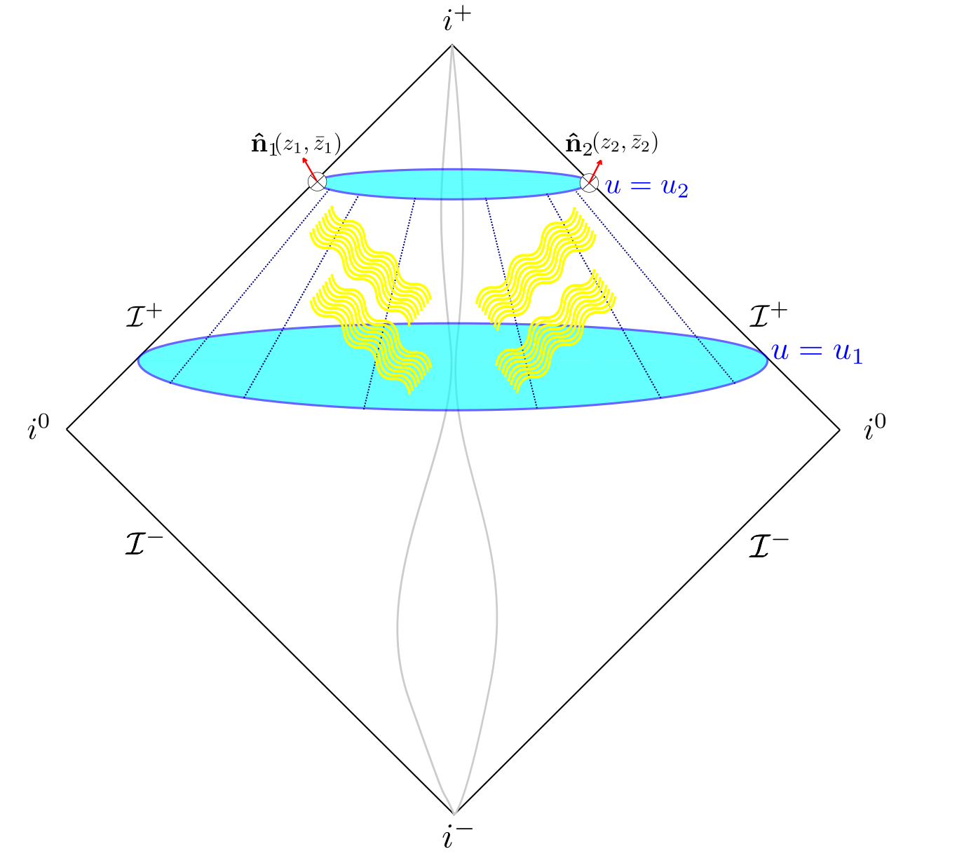
Figure 1: The radiation due to the scattering of two massive objects is captured by two detectors located at spatial infinity in the directions $\hat{\mathbf{n}}_{1}(z_{1},\bar{z}_{1})$ and $\hat{\mathbf{n}}_{2}(z_{2},\bar{z}_{2})$.

In the case of two (or more) detectors, as previously mentioned, we can also define the energy-energy correlator which is related to the 2-pt Wightman function of two ANEC operators at infinity (8) inserted at different points on the celestial sphere

$$\langle\mathcal{\tilde{E}}(\hat{\mathbf{n}})\mathcal{\tilde{E}}(\hat{\mathbf{n}}^{\prime})\rangle:=\frac{1}{\sigma_{\text{tot}}(p_{1},p_{2})}\left<\mathbf{p}_{1}\mathbf{p}_{2}\right|S^{\dagger}\mathcal{\tilde{E}}(\hat{\mathbf{n}})\mathcal{\tilde{E}}(\hat{\mathbf{n}}^{\prime})S\left|\mathbf{p}_{1}\mathbf{p}_{2}\right>.$$ (12)

It is quite interesting to analyze this 2-pt correlator for the gravitational radiation in the classical limit, where in the most general case a superposition of coherent states represents the radiation at the quantum level.

In flat null coordinates the momentum flow operator can be written directly in terms of the energy flow

$$\mathcal{P}^{\mu}(\hat{\mathbf{n}})=n^{\mu}\mathcal{E}(\hat{\mathbf{n}})=n^{\mu}\int_{-\infty}^{+\infty}\mathrm{d}u\,\lim_{r\to\infty}r^{2}T_{uu}(u,r,z_{\hat{\mathbf{n}}},\bar{z}_{\hat{\mathbf{n}}}),$$ (13)

where $u$ is the retarded time and identify $\hat{\mathbf{n}}$ with the related coordinates on the celestial sphere

$$\hat{\mathbf{n}}\Leftrightarrow(z_{\hat{\mathbf{n}}},\bar{z}_{\hat{\mathbf{n}}}).$$ (14)

Here, we emphasize that we use $\mathcal{E}(\hat{\mathbf{n}})$ in place of $\mathcal{\tilde{E}}(\hat{\mathbf{n}})$ for technical convenience. One can work in Bondi gauge where the detector would register the energy flow as given by $\mathcal{\tilde{E}}(\hat{\mathbf{n}})$ (i.e. the standard local energy factor). We will do this later on for gravitational event shapes.

2 Light-ray operators in QFT

In this section, we define the family of light-ray operators under consideration and make contact with their physical significance and in particular with the corresponding surface charges of null-sheet symmetry generators. Light-ray operators depend implicitly on a choice of null-sheet and we choose future null infinity.

In flat-null coordinates, our family of light-ray operators is defined by

$$\mathcal{E}(\hat{\mathbf{n}}) =\int_{-\infty}^{+\infty}\mathrm{d}u\,\lim_{r\to\infty}r^{2}T_{uu}(u,r,z_{\hat{\mathbf{n}}},\bar{z}_{\hat{\mathbf{n}}}),$$

$$\mathcal{K}(\hat{\mathbf{n}}) =\int_{-\infty}^{+\infty}\mathrm{d}u\,u\lim_{r\to\infty}r^{2}T_{uu}(u,r,z_{\hat{\mathbf{n}}},\bar{z}_{\hat{\mathbf{n}}}),$$

$$\mathcal{N}_{z}(\hat{\mathbf{n}}) =\int_{-\infty}^{+\infty}\mathrm{d}u\,\lim_{r\to\infty}r^{2}T_{uz}(u,r,z_{\hat{\mathbf{n}}},\bar{z}_{\hat{\mathbf{n}}}),$$

$$\mathcal{N}_{\bar{z}}(\hat{\mathbf{n}}) =\int_{-\infty}^{+\infty}\mathrm{d}u\,\lim_{r\to\infty}r^{2}T_{u\bar{z}}(u,r,z_{\hat{\mathbf{n}}},\bar{z}_{\hat{\mathbf{n}}}).$$ (15)

We will collectively denote these operators by $L(\hat{\mathbf{n}})=\{\mathcal{E}(\hat{\mathbf{n}}),\mathcal{K}(\hat{\mathbf{n}}),\mathcal{N}_{z}(\hat{\mathbf{n}}),\mathcal{N}_{\bar{z}}(\hat{\mathbf{n}})\}$.

This family of light-ray operators can be understood as surface densities for the corresponding conserved charges of the future null boundary of Minkowski spacetime. To see this, consider an affine transformation of the null surface generator Wall:2011hj

$$\delta u=A+B\,u,$$ (16)

where $A$ and $B$ are arbitrary constants. Since $\lim_{r\to\infty}r^{2}T_{uu}(u,r,z,\bar{z})$ corresponds to the generator of null diffeomorphisms, we can integrate it to obtain either the generator of null translation $\delta u=A$

$$\frac{1}{2}\int_{-\infty}^{+\infty}\mathrm{d}u\int\mathrm{d}^{2}z\,\lim_{r\to\infty}r^{2}T_{uu}(u,r,z,\bar{z})$$ (17)

or of dilatations $\delta u=B\,u$

$$\frac{1}{2}\int_{-\infty}^{+\infty}\mathrm{d}u\int\mathrm{d}^{2}z\,u\lim_{r\to\infty}r^{2}T_{uu}(u,r,z,\bar{z}),$$ (18)

which is an equivalent definition of $\int\mathrm{d}^{2}z\,\mathcal{K}(z,\bar{z})$. The latter is called “boost mass” $M_{\text{boost}}$ in the literature and it is usually defined for null-like horizons using the boost Killing vector of a causal wedge in Minkowski spacetime Jacobson:1995ab ; Wall:2010cj ; Wall:2011hj . In a CFT, this provides a direct connection to the concept of modular hamiltonian for null-like horizons Casini:2017roe . While for empty Minkowski spacetime the boost mass is exactly zero, for more general non-asymptotically flat spacetimes it might be relevant for a proper formulation of the first law of black hole thermodynamics Dutta:2005iy . In particular, it turns out that while the ADM mass $M_{\text{ADM}}$ measures the total “monopole” distribution of the matter in the spacetime, the boost mass $M_{\text{boost}}$ measures the total “dipole” moment of the mass distribution at infinity Dutta:2005iy .

Since we are only considering QFTs on a flat Minkowski background, we will not delve deeper into these topics. However, we will find the monopole versus dipole distinction relevant for understanding the action of $\mathcal{K}(\hat{\mathbf{n}})$ on on-shell states. From now on, we will call $\mathcal{K}(\hat{\mathbf{n}})$ the boost energy (surface) density. In the same spirit, the ANEC at infinity can be called null energy (surface) density.

Following a similar line of reasoning one finds that $\mathcal{N}_{z}(\hat{\mathbf{n}})$ and $\mathcal{N}_{\bar{z}}(\hat{\mathbf{n}})$ are associated to the local vector fields $\partial_{z}$ and $\partial_{\bar{z}}$, i.e. with the angular momentum flux charge

$$\frac{1}{2}\int_{-\infty}^{+\infty}\mathrm{d}u\int\mathrm{d}^{2}z\,\lim_{r\to\infty}r^{2}T_{uz}(u,r,z,\bar{z})\,,\qquad\frac{1}{2}\int_{-\infty}^{+\infty}\mathrm{d}u\int\mathrm{d}^{2}z\,\lim_{r\to\infty}r^{2}T_{u\bar{z}}(u,r,z,\bar{z}).$$ (20)

Therefore $\mathcal{N}_{z}(\hat{\mathbf{n}})$ and $\mathcal{N}_{\bar{z}}(\hat{\mathbf{n}})$ can be thought as angular momentum flux (surface) densities. More generally, this family of non-local light-ray operators appear naturally in Einstein equations solved near null infinity and in particular in (BMS and Poincaré) balance flux laws Compere:2019gft , where they represent the radiative contribution to the fluxes.

Here we interpret physically the insertion of our light-ray operators as an insertion of a physical detector on the boundary of Minkowski spacetime. We will be interested in how these operators act on on-shell states and we will then compute their expectation values in perturbation theory, as in the standard event shapes literature.

3 The Spin-0 light-ray operators

Here, we consider a theory of self-interacting massless scalars with a potential $Q(\phi)$ that is polynomial in the fields and without derivative interactions. We derive explicit expressions for our family of light-ray operators in terms of the scalar creation and annihilation operators.

The Hilbert stress tensor $T^{\text{matter}}_{\mu\nu}=-\frac{2}{\sqrt{|g|}}\frac{\delta S^{\text{matter}}}{\delta g^{\mu\nu}}$ for our theory of scalars is simply

$$T_{\mu\nu}^{\text{scalar}}=(\partial_{\mu}\phi)(\partial_{\nu}\phi)-\eta_{\mu\nu}\left(\frac{1}{2}\partial_{\alpha}\phi\partial^{\alpha}\phi-Q(\phi)\right).$$ (21)

The scalar stress tensor components which are relevant for the light-ray operators are

$$T^{\text{scalar}}_{uu}(x){=}(\partial_{u}\phi)(\partial_{u}\phi),\qquad T^{\text{scalar}}_{uz}(x){=}(\partial_{u}\phi)(\partial_{z}\phi),\qquad T^{\text{scalar}}_{u\bar{z}}(x){=}(\partial_{u}\phi)(\partial_{\bar{z}}\phi).$$ (22)

The next step is to substitute the leading term in the large $r$ expansion of the scalar field into the expressions above. However, to do this, we need to impose some boundary conditions on the field.

Since we require the energy flux across $\mathcal{I}^{+}$ to be finite, we impose the following falloff condition for the scalar field

$$\phi(u,r,z,\bar{z}) =\frac{\phi^{(0)}(u,z,\bar{z})}{r}+\mathcal{O}\left(\frac{1}{r}\right),\qquad\lim_{u\to\pm\infty}\phi^{(0)}(u,z,\bar{z})=0.$$ (23)

Far away from interactions we can safely use the free field mode expansion

$$\phi(x)=\int\widetilde{\mathrm{d}^{3}p}\left[b(\mathbf{p})e^{-ip\cdot x}+b^{\dagger}(\mathbf{p})e^{ip\cdot x}\right]$$ (24)

and evaluate the field with the large $r$ saddle-point estimate. Physically, $r$ is the distance from the detector to the region where the interaction is localized and it should be much larger than the inverse of the smallest momentum scale that appears in the S-matrix Bauer:2008dt . Note that in our coordinate conventions the canonical commutators read

$$[b(\mathbf{p}),b^{\dagger}(\mathbf{q})]=\frac{4(2\pi)^{3}}{\omega_{p}}\delta(\omega_{p}-\omega_{q})\delta^{2}(z_{\hat{\mathbf{p}}}-z_{\hat{\mathbf{q}}}).$$ (25)

The large $r$ limit of such a Fourier integral is controlled by the exponents of the exponentials

$$f(z,w):=ip\cdot x=i\frac{\omega_{p}u}{2}+i\frac{\omega_{p}r}{2}|z-w|^{2},$$ (26)

where we use

$$x^{\mu} =\frac{r}{2}\left(1+z\bar{z}+\frac{u}{r},z+\bar{z},-i(z-\bar{z}),1-z\bar{z}-\frac{u}{r}\right),$$

$$p^{\mu} =\frac{\omega_{p}}{2}\left(1+w\bar{w},w+\bar{w},-i(w-\bar{w}),1-w\bar{w}\right).$$ (27)

as our parametrization for the coordinates and on-shell momentum He:2019jjk ; He:2020ifr . The only saddle point is at $(z,\bar{z})=(w,\bar{w})$. Making the following change of variables $(y_{1},y_{2})=\left(\frac{1}{2}(z+\bar{z}),-\frac{i}{2}(z-\bar{z})\right)$ brings the exponentials into Gaussian form, which integrates to

$$\frac{1}{2}\int\mathrm{d}^{2}z\,e^{-i\frac{\omega_{p}r}{2}(z-w)(\bar{z}-\bar{w})}=\int\mathrm{d}y_{1}\mathrm{d}y_{2}\,e^{-i\frac{\omega_{p}r}{2}(y_{1}^{2}+y_{2}^{2})}=\frac{(2\pi)(-i)}{r\omega}.$$ (28)

Substituting into the mode expansion for $\phi(x)$ yields the leading term in the large $r$ limit

$$\phi^{(0)}(u,\hat{\mathbf{n}})=\frac{i}{(8\pi^{2})}\int_{0}^{+\infty}\mathrm{d}\omega\,\left[b^{\dagger}(\omega,z_{\hat{\mathbf{n}}},\bar{z}_{\hat{\mathbf{n}}})e^{i\frac{\omega u}{2}}-b(\omega,z_{\hat{\mathbf{n}}},\bar{z}_{\hat{\mathbf{n}}})e^{-i\frac{\omega u}{2}}\right].$$ (29)

When derivatives in $z$ (or $\bar{z}$) acts on field operators expressions, one can write

$$\partial_{z}\phi^{(0)}(u,\hat{\mathbf{n}}) =\frac{i}{(8\pi^{2})}\int_{0}^{+\infty}\mathrm{d}\omega_{p}\,\left[\partial_{z_{\hat{\mathbf{n}}}}b^{\dagger}(\omega_{p},z_{\hat{\mathbf{n}}},\bar{z}_{\hat{\mathbf{n}}})e^{i\frac{\omega_{p}u}{2}}-\partial_{z_{\hat{\mathbf{n}}}}b(\omega_{p},z_{\hat{\mathbf{n}}},\bar{z}_{\hat{\mathbf{n}}})e^{-i\frac{\omega_{p}u}{2}}\right]$$ (30)

for the saddle point estimate of $\partial_{z}\phi^{(0)}$ where the derivative acts on the creation and annihilation operators localized around $(w,\bar{w})=(z_{\hat{\mathbf{n}}},\bar{z}_{\hat{\mathbf{n}}})$.

Inserting the saddle point estimate of $\phi(x)$ into the definition for the scalar ANEC operator at infinity, we find

$$\mathcal{E}_{\text{scalar}}(\hat{\mathbf{n}}) =\int\widetilde{\mathrm{d}^{3}p}\;\omega_{p}\,:b^{\dagger}(\mathbf{p})b(\mathbf{p}):\delta^{2}(z_{\hat{\mathbf{n}}}-z_{\hat{\mathbf{p}}}),$$ (31)

where we have set to zero all contributions proportional to $\delta(\omega_{p_{1}}+\omega_{p_{2}})$ since the only cases that these constraints can be satisfied correspond to $\omega_{p_{1}}\to 0^{\pm}$ and $\omega_{p_{2}}\to 0^{\mp}$, which are unphysical. The action of $\mathcal{E}_{\text{scalar}}(\hat{\mathbf{n}})$ on an on-shell state $\left|\mathbf{X}\right>=\left|\mathbf{p}_{1}...\mathbf{p}_{n}\right>$ gives

$$\mathcal{E}_{\text{scalar}}(\hat{\mathbf{n}})\left|\mathbf{X}\right>=\sum_{i=1}^{n}\left(\omega_{i}\right)\delta^{2}(z_{\hat{\mathbf{n}}}-z_{\hat{\mathbf{p}}_{i}})\left|\mathbf{X}\right>,$$ (32)

which is natural for an observer located at spatial infinity who is measuring the energy flux along the retarded time $u$ in flat null coordinates. Note that on-shell scattering states are eigenstates of the ANEC operator in the detector limit whose eigenvalues are weight functions similar to equation (7).

Inserting (29) into the definition of the boost energy density flux $\mathcal{K}_{\text{scalar}}(\hat{\mathbf{n}})$ yields

$$\mathcal{K}_{\text{scalar}}(\hat{\mathbf{n}})=\int_{-\infty}^{+\infty}\mathrm{d}u\,(u)\lim_{r\to\infty}r^{2}\,\prod_{i=1}^{2}\left[\int_{0}^{+\infty}\mathrm{d}\omega_{p_{i}}\,\frac{\omega_{p_{i}}}{2(8\pi^{2})r}\right]$$

$$\times:\Big{[}b^{\dagger}(\omega_{p_{1}}\hat{\mathbf{n}})b(\omega_{p_{2}}\hat{\mathbf{n}})e^{-i\frac{(\omega_{p_{2}}-\omega_{p_{1}})}{2}u}+b(\omega_{p_{1}}\hat{\mathbf{n}})b(\omega_{p_{2}}\hat{\mathbf{n}})e^{-i\frac{(\omega_{p_{1}}+\omega_{p_{2}})}{2}u}+h.c.\Big{]}:.$$ (33)

It is convenient to change variables

$$\omega_{-}:=\frac{\omega_{p_{1}}-\omega_{p_{2}}}{2}\qquad\omega_{+}:=\frac{\omega_{p_{1}}+\omega_{p_{2}}}{2},$$ (34)

where $\omega_{+}\in[\text{max}\{-\omega_{-},\omega_{-}\},+\infty[$ and $\omega_{-}\in]-\infty,+\infty[$ is a convenient slicing of the integration region in the new variables. In the new variables,

$$\mathcal{K}_{\text{scalar}}(\hat{\mathbf{n}}) =\frac{(-i)}{8}\int_{-\infty}^{+\infty}\frac{\mathrm{d}\omega_{-}}{(2\pi)^{3}}\delta^{(1)}(\omega_{-})\int_{\text{max}\{-\omega_{-},\omega_{-}\}}^{+\infty}\mathrm{d}\omega_{+}\,((\omega_{+})^{2}-(\omega_{-})^{2})$$

$$\hskip 100.0pt\times:\Big{[}b^{\dagger}\left((\omega_{+}+\omega_{-})\hat{\mathbf{n}}\right)b\left((\omega_{+}-\omega_{-})\hat{\mathbf{n}}\right)-h.c.\Big{]}:,$$ (35)

where we have used the following distributional identity (for $n=1$)

$$\int\mathrm{d}u\,(u)^{n}e^{i\omega_{-}u} =(2\pi)(-i)^{n}\delta^{(n)}(\omega_{-}).$$ (36)

The derivative acting on the energy delta function might seem troubling at first sight. To develop more intuition, we study the action of this operator on on-shell states $\left|\mathbf{X}\right>=\left|\mathbf{p}_{1}...\mathbf{p}_{n}\right>$:

$$\mathcal{K}_{\text{scalar}}(\hat{\mathbf{n}})\left|\mathbf{X}\right>=\frac{(-i)}{4}\int_{-\infty}^{+\infty}\frac{\mathrm{d}\omega_{-}}{(2\pi)^{3}}\delta^{(1)}(\omega_{-})\int_{\text{max}\{-\omega_{-},\omega_{-}\}}^{+\infty}\mathrm{d}\omega_{+}\,((\omega_{+})^{2}-(\omega_{-})^{2})$$

$$\qquad\times\sum_{i=1}^{n}(2\pi)^{3}\frac{4}{\omega_{p_{i}}}\delta\left((\omega_{+}-\omega_{-})-\omega_{p_{i}}\right)\delta^{2}(z_{\hat{\mathbf{n}}}-z_{\hat{\mathbf{p}}_{i}})\left|\mathbf{p}_{1}...\underbrace{(\omega_{+}+\omega_{-})\hat{\mathbf{n}}}_{\text{i-th}}...\mathbf{p}_{n}\right>.$$ (37)

Then one can solve the $\omega_{+}$ integral

$$\mathcal{K}_{\text{scalar}}(\hat{\mathbf{n}})\left|\mathbf{X}\right>=2\sum_{i=1}^{n}\delta^{2}(z_{\hat{\mathbf{n}}}-z_{\hat{\mathbf{p}}_{i}})\int_{-\omega_{p_{i}}}^{+\infty}\mathrm{d}\omega(-i\delta^{(1)}(\omega))\,\left(\omega_{p_{i}}+\omega\right)\left|\mathbf{p}_{1}...\underbrace{(\omega_{p_{i}}+\omega)\hat{\mathbf{n}}}_{\text{i-th}}...\mathbf{p}_{n}\right>,$$ (38)

where we have relabelled $\omega_{-}$ as $\omega$. It is also enlightening to compare the simplest matrix elements of $\mathcal{E}_{\text{scalar}}(\hat{\mathbf{n}})$ and $\mathcal{K}_{\text{scalar}}(\hat{\mathbf{n}})$

$$\left<\mathbf{q}\right|\mathcal{E}_{\text{scalar}}(\hat{\mathbf{n}})\left|\mathbf{p}\right> =4(2\pi)^{3}\delta^{2}(z_{\hat{\mathbf{n}}}-z_{\hat{\mathbf{p}}})\delta^{2}(z_{\hat{\mathbf{q}}}-z_{\hat{\mathbf{n}}})\delta(\omega_{q}-\omega_{p}),$$

$$\left<\mathbf{q}\right|\mathcal{K}_{\text{scalar}}(\hat{\mathbf{n}})\left|\mathbf{p}\right> =2\delta^{2}(z_{\hat{\mathbf{n}}}-z_{\hat{\mathbf{p}}})\int_{-\omega_{p}}^{+\infty}\mathrm{d}\omega(-i\delta^{(1)}(\omega))\,\left(\omega_{p}+\omega\right)\left<\mathbf{q}\vphantom{(\omega_{p}+\omega)\hat{\mathbf{n}}}\right|\left.(\omega_{p}+\omega)\hat{\mathbf{n}}\vphantom{\mathbf{q}}\right>$$

$$=8(2\pi)^{3}\delta^{2}(z_{\hat{\mathbf{n}}}-z_{\hat{\mathbf{p}}})\delta^{2}(z_{\hat{\mathbf{q}}}-z_{\hat{\mathbf{n}}})(-i\delta^{(1)}(\omega_{q}-\omega_{p})).$$ (39)

It is well-known that in QFT the single contraction $\left<\mathbf{q}\vphantom{\mathbf{p}}\right|\left.\mathbf{p}\vphantom{\mathbf{q}}\right>$ must be interpreted in a distributional sense; in order to properly define such objects one needs to smear them with a well-behaved function (see Collins:2019ozc ; Duncan:1493543 and references therein). In the S-matrix context, one usually considers outgoing states of the form

$$\left|\psi_{\mathbf{p},\text{out}}\right>=\int\widetilde{\mathrm{d}^{3}\tilde{p}}\;\phi_{\mathbf{p}}(\tilde{\mathbf{p}})\left|\tilde{\mathbf{p}}\right>,$$ (40)

where $\phi_{\mathbf{p}}(\tilde{\mathbf{p}})$ is a suitable real momentum wavefunction localized around $\mathbf{p}$. Note that $\left|\psi_{\mathbf{p},\text{out}}\right>\to\left|\mathbf{p}\right>$ when $\phi_{\mathbf{p}}(\tilde{\mathbf{p}})\to(2\pi)^{3}(2E_{p})\delta^{3}(\mathbf{p}-\tilde{\mathbf{p}})$. More generally, when $\phi_{\mathbf{p}}(\tilde{\mathbf{p}})$ is sufficiently smooth (39) is well defined

$$\left<\psi_{\mathbf{q},\text{out}}\right|\mathcal{E}_{\text{scalar}}(\hat{\mathbf{n}})\left|\psi_{\mathbf{p},\text{out}}\right> =4(2\pi)^{3}\int\widetilde{\mathrm{d}^{3}\tilde{p}}\;\int\widetilde{\mathrm{d}^{3}\tilde{q}}\;\phi_{\mathbf{p}}(\tilde{\mathbf{p}})\phi_{\mathbf{q}}(\tilde{\mathbf{q}})$$

$$\hskip 60.0pt\times\delta(\omega_{\tilde{q}}-\omega_{\tilde{p}})\delta^{2}(z_{\hat{\mathbf{n}}}-z_{\hat{\tilde{\mathbf{p}}}})\delta^{2}(z_{\hat{\tilde{\mathbf{q}}}}-z_{\hat{\mathbf{n}}}),$$

$$\left<\psi_{\mathbf{q},\text{out}}\right|\mathcal{K}_{\text{scalar}}(\hat{\mathbf{n}})\left|\psi_{\mathbf{p},\text{out}}\right> =8(2\pi)^{3}\int\widetilde{\mathrm{d}^{3}\tilde{p}}\;\int\widetilde{\mathrm{d}^{3}\tilde{q}}\;\phi_{\mathbf{p}}(\tilde{\mathbf{p}})\phi_{\mathbf{q}}(\tilde{\mathbf{q}})$$

$$\hskip 60.0pt\times(-i\delta^{(1)}(\omega_{\tilde{q}}-\omega_{\tilde{p}}))\delta^{2}(z_{\hat{\mathbf{n}}}-z_{\hat{\tilde{\mathbf{p}}}})\delta^{2}(z_{\hat{\tilde{\mathbf{q}}}}-z_{\hat{\mathbf{n}}}).$$ (41)

Looking at (41), the interpretation of $\mathcal{K}_{\text{scalar}}(\hat{\mathbf{n}})$ is also much more clear: while $\delta(\omega_{\tilde{q}}-\omega_{\tilde{p}})$ can be considered the limit of a suitable localized function around $\omega_{\tilde{q}}=\omega_{\tilde{p}}$, it turns out that $\delta^{(1)}(\omega_{\tilde{q}}-\omega_{\tilde{p}})$ is probing a dipole-like pattern around $\omega_{\tilde{q}}=\omega_{\tilde{p}}$ (see 2(a) and 2(b) respectively).

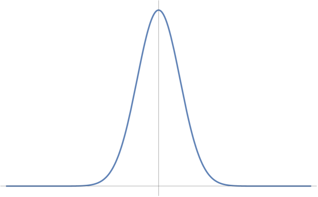
(a) Standard Gaussian shape peaked around $\omega_{\tilde{q}}=\omega_{\tilde{p}}$, which converges to $\delta(\omega_{\tilde{q}}-\omega_{\tilde{p}})$ in the limit of zero width.

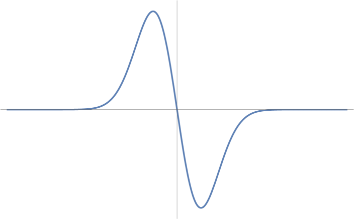
(b) Dipole profile centered around $\omega_{\tilde{q}}=\omega_{\tilde{p}}$, which converges to $\delta^{(1)}(\omega_{\tilde{q}}-\omega_{\tilde{p}})$ in the limit of zero width.

Figure 2: Comparison of the expectation values of $\left<\psi_{\mathbf{q},\text{out}}\right|\mathcal{E}_{\text{scalar}}(\hat{\mathbf{n}})\left|\psi_{\mathbf{p},\text{out}}\right>$ and $\left<\psi_{\mathbf{q},\text{out}}\right|\mathcal{K}_{\text{scalar}}(\hat{\mathbf{n}})\left|\psi_{\mathbf{p},\text{out}}\right>$ as a function of the energy $\omega$.

The final operator we consider is $\mathcal{N}_{z,\text{scalar}}(\hat{\mathbf{n}})$, which after using (29) and (30) is

$$\mathcal{N}_{z,\text{scalar}}(\hat{\mathbf{n}}) =\frac{i}{4(2\pi)^{3}}\int\mathrm{d}\omega_{p}\,\omega_{p}:\Big{[}b^{\dagger}\left(\omega_{p},z_{\hat{\mathbf{n}}},\bar{z}_{\hat{\mathbf{n}}}\right)\partial_{z_{\hat{\mathbf{n}}}}b\left(\omega_{p},z_{\hat{\mathbf{n}}},\bar{z}_{\hat{\mathbf{n}}}\right)$$

$$\hskip 120.0pt-b\left(\omega_{p},z_{\hat{\mathbf{n}}},\bar{z}_{\hat{\mathbf{n}}}\right)\partial_{z_{\hat{\mathbf{n}}}}b^{\dagger}\left(\omega_{p},z_{\hat{\mathbf{n}}},\bar{z}_{\hat{\mathbf{n}}}\right)\Big{]}:.$$ (42)

More compactly,

$$\mathcal{N}_{z,\text{scalar}}(\hat{\mathbf{n}})=i\int\widetilde{\mathrm{d}^{3}p}\,\delta^{2}\left(z_{\hat{\mathbf{n}}}-z_{\hat{\mathbf{p}}}\right):\left[b^{\dagger}(\omega_{p}\hat{\mathbf{n}})\overset{\leftrightarrow}{\partial}_{z_{\hat{\mathbf{n}}}}b(\omega_{p}\hat{\mathbf{n}})\right]:,$$ (43)

where

$$\frac{i}{2}\partial_{z}=L_{uz}=\frac{i}{r}\left(\partial_{u}x^{\mu}\right)\left(\partial_{z}x^{\nu}\right)\left[p_{\mu}\frac{\partial}{\partial p^{\nu}}-p_{\nu}\frac{\partial}{\partial p^{\mu}}\right]$$ (44)

is the standard orbital angular momentum operator. A similar analysis can be repeated for the antiholomorphic component by flipping $z\leftrightarrow\bar{z}$.

4 The Spin-1 light-ray operators

Having found explicit expressions for the light-ray operators for massless scalar theories, we now derive similar results for the light-ray operators for massless spin-1 theories. Using the Hilbert stress tensor $T^{\text{matter}}_{\mu\nu}=-\frac{2}{\sqrt{|g|}}\frac{\delta S^{\text{matter}}}{\delta g^{\mu\nu}}$ for pure gauge theories, one obtains

$$T^{\mu\nu}_{\text{photon}}=F^{\mu\alpha}F^{\,\,\nu}_{\alpha}+\frac{1}{4}\eta^{\mu\nu}F^{\alpha\beta}F_{\alpha\beta}$$ (45)

for Maxwell $U(1)$ theory where $F_{\mu\nu}:=\partial_{\mu}A_{\nu}-\partial_{\nu}A_{\mu}$ is the $U(1)$ field strength. The generalization to the non-abelian gauge group $SU(N)$ is straightforward

$$T^{\mu\nu}_{\text{gluon}}=2\text{Tr}(T^{a}T^{b})\left[(F^{a})^{\mu\alpha}(F^{b})^{\,\,\nu}_{\alpha}+\frac{1}{4}\eta^{\mu\nu}(F^{a})^{\alpha\beta}(F^{b})_{\alpha\beta}\right],$$ (46)

where $F^{a}_{\mu\nu}:=\partial_{\mu}A^{a}_{\nu}-\partial_{\nu}A^{a}_{\mu}+gf^{abc}A^{b}_{\mu}A^{c}_{\nu}$ is the $SU(N)$ field strength. Here, the $SU(N)$ generators are chosen to be hermitian $[T^{a},T^{b}]=if^{abc}T^{c}$ and are normalized according to $\text{Tr}(T^{a}T^{b})=\frac{1}{2}\delta^{ab}$.

To discuss the large $r$ limit of the stress-tensor, we need the large $r$ limit of the gauge field, which requires making a gauge choice, as well as, specifying boundary conditions. We will adopt the radiation gauge Strominger:2013lka

$$A_{u}=0,\qquad\left.r^{2}\nabla^{\mu}A_{\mu}^{a}(x)\right|_{\mathcal{I}-}=\left.2\left[r^{2}\partial_{u}A_{r}^{a}-\partial_{z}A_{\bar{z}}^{a}-\partial_{\bar{z}}A_{z}^{a}\right]\right|_{\mathcal{I}^{-}}=0$$ (47)

and we require the gauge field components to satisfy the following falloff conditions at infinity

$$A_{z}(u,r,z,\bar{z})=A_{z}^{(0)}(u,z,\bar{z})+\mathcal{O}\left(\frac{1}{r}\right),\qquad A_{r}(u,r,z,\bar{z})=\frac{1}{r^{2}}A_{r}^{(2)}(u,z,\bar{z})+\mathcal{O}\left(\frac{1}{r^{3}}\right),$$ (48)

which are needed to have a finite energy and angular momentum flux at $\mathcal{I}^{+}$. The stress tensor components relevant for our family of light-ray operators (46) are

$$T_{uu} =\frac{4}{r^{2}}(\partial_{u}A_{z}^{(0),a})(\partial_{u}A_{\bar{z}}^{(0),a}),$$ (49)

$$T_{uz} =\frac{2}{r^{2}}(\partial_{u}A_{z}^{(0),a})(2\partial_{[z}A_{\bar{z}]}^{(0),a}+gf^{abc}A_{z}^{(0),b}A_{\bar{z}}^{(0),c})+\frac{2}{r^{2}}(\partial_{u}A_{z}^{(0),a})(\partial_{u}A_{r}^{(2),a}),$$ (50)

$$T_{u\bar{z}} =\frac{2}{r^{2}}(\partial_{u}A_{\bar{z}}^{(0),a})(2\partial_{[\bar{z}}A_{z]}^{(0),a}+gf^{abc}A_{\bar{z}}^{(0),b}A_{z}^{(0),c})+\frac{2}{r^{2}}(\partial_{u}A_{\bar{z}}^{(0),a})(\partial_{u}A_{r}^{(2),a})$$ (51)

up to terms of order $\mathcal{O}(1/r^{3})$.

We assume that we can work perturbatively with energies above the confinement scale $\Lambda>0$ and can formally talk about asymptotic gluon states. We use the following parametrization and projection of the polarization vectors

$$\epsilon^{+,\mu}(\mathbf{q}) =\frac{1}{\sqrt{2}}(\bar{z}_{q},1,-i,-\bar{z}_{q}),\qquad\epsilon^{-,\mu}(\mathbf{q})=\frac{1}{\sqrt{2}}(z_{q},1,i,-z_{q}),$$

$$(\partial_{z}x^{\mu})\epsilon_{\mu}^{+}(\mathbf{q}) =0=(\partial_{\bar{z}}x^{\mu})\epsilon_{\mu}^{-}(\mathbf{q}),\qquad(\partial_{z}x^{\mu})\epsilon_{\mu}^{-}(\mathbf{q})=-\frac{r}{\sqrt{2}}=(\partial_{\bar{z}}x^{\mu})\epsilon_{\mu}^{+}(\mathbf{q})$$ (52)

and the canonical commutation relations

$$[a_{\sigma}(\mathbf{p}),a^{\dagger}_{\sigma^{\prime}}(\mathbf{q})]=\frac{4(2\pi)^{3}}{\omega_{p}}\delta_{\sigma\sigma^{\prime}}\delta(\omega_{p}-\omega_{q})\delta^{2}(z_{\hat{\mathbf{p}}}-z_{\hat{\mathbf{q}}}).$$ (53)

Starting with the gluon-ANEC operator at null infinity, we find

$$\mathcal{E}_{\text{gluon}}(\hat{\mathbf{n}})=\int\widetilde{\mathrm{d}^{3}p}\,\,\omega_{p}\,\delta^{2}(z_{\hat{\mathbf{n}}}-z_{\hat{\mathbf{p}}})\sum_{\sigma=\pm 1}:\Big{[}a^{\dagger,a}_{\sigma}(\omega_{p}\hat{\mathbf{n}})a^{a}_{\sigma}(\omega_{p}\hat{\mathbf{n}})\Big{]}:,$$ (54)

where the saddle point estimates for $A_{z}^{(0),a}$ and $A_{\bar{z}}^{(0),a}$ are

$$A_{z}^{(0),a}(u,\hat{\mathbf{n}}) =\frac{-i}{(8\sqrt{2}\pi^{2})}\int_{0}^{+\infty}\mathrm{d}\omega_{p}\,\left[a^{\dagger,a}_{-}(\omega_{p}\hat{\mathbf{n}})e^{i\frac{\omega_{p}u}{2}}-a^{a}_{+}(\omega_{p}\hat{\mathbf{n}})e^{-i\frac{\omega_{p}u}{2}}\right],$$ (55)

$$A_{\bar{z}}^{(0),a}(u,\hat{\mathbf{n}}) =\frac{-i}{(8\sqrt{2}\pi^{2})}\int_{0}^{+\infty}\mathrm{d}\omega_{p}\,\left[a^{\dagger,a}_{+}(\omega_{p}\hat{\mathbf{n}})e^{i\frac{\omega_{p}u}{2}}-a^{a}_{-}(\omega_{p}\hat{\mathbf{n}})e^{-i\frac{\omega_{p}u}{2}}\right].$$ (56)

Analogous to the scalar case, on-shell gluon states $\left|\mathbf{X}\right>=\left|\{\mathbf{p}_{1},\sigma_{1}\},...,\{\mathbf{p}_{n},\sigma_{n}\}\right>$ are eigenstates of the gluon-ANEC at infinity

$$\mathcal{E}_{\text{gluon}}(\hat{\mathbf{n}})\left|\mathbf{X}\right>=\sum_{i=1}^{n}\left(\omega_{i}\right)\delta^{2}(z_{\hat{\mathbf{n}}}-z_{\hat{\mathbf{p}}_{i}})\left|\mathbf{X}\right>.$$ (57)

The gluon boost energy density operator $\mathcal{K}_{\text{gluon}}(\hat{\mathbf{n}})$ follows straightforwardly

$$\mathcal{K}_{\text{gluon}}(\hat{\mathbf{n}}) =\frac{(-i)}{4}\int_{-\infty}^{+\infty}\frac{\mathrm{d}\omega_{-}}{(2\pi)^{3}}\delta^{(1)}(\omega_{-})\int_{\text{max}\{-\omega_{-},\omega_{-}\}}^{+\infty}\mathrm{d}\omega_{+}\,((\omega_{+})^{2}-(\omega_{-})^{2})$$

$$\hskip 90.0pt\times\sum_{\sigma=\pm 1}:\Big{[}a_{\sigma}^{a,\dagger}\left((\omega_{+}+\omega_{-})\hat{\mathbf{n}}\right)a^{a}_{\sigma}\left((\omega_{+}-\omega_{-})\hat{\mathbf{n}}\right)\Big{]}:.$$ (58)

These operators are especially simple; the only fundamental difference between
$\{\mathcal{E}_{\text{gluon}},\mathcal{K}_{\text{gluon}}\}$ and $\{\mathcal{E}_{\text{scalar}},\mathcal{K}_{\text{scalar}}\}$ is the sum over helicities.

On the other hand, the spin-1 angular momentum flux operators are complicated by boundary terms, which come from integrating by parts in $u$. Explicitly,

$$\int\mathrm{d}u\lim_{r\to+\infty}r^{2}T_{uz}$$

$$\qquad=\int\mathrm{d}u\Big{\{}4(\partial_{u}A_{z}^{(0),a})(\partial_{z}A_{\bar{z}}^{(0),a})\Big{\}}-2A_{z}^{(0),a}(-\partial_{u}A_{r}^{(2),a}+\partial_{z}A_{\bar{z}}^{(0),a}+\partial_{\bar{z}}A_{z}^{(0),a})\Big{|}_{\mathcal{I}^{+}_{+}},$$

$$\int\mathrm{d}u\lim_{r\to+\infty}r^{2}T_{u\bar{z}}$$

$$\qquad=\int\mathrm{d}u\Big{\{}4(\partial_{u}A_{\bar{z}}^{(0),a})(\partial_{\bar{z}}A_{z}^{(0),a})\Big{\}}-2A_{\bar{z}}^{(0),a}(-\partial_{u}A_{r}^{(2),a}+\partial_{z}A_{\bar{z}}^{(0),a}+\partial_{\bar{z}}A_{z}^{(0),a})\Big{|}_{\mathcal{I}^{+}_{+}},$$ (59)

where we have used the leading $u$-equation of motion

$$r^{2} \mathcal{D}_{\mu}F^{\mu}_{\,\,\,u}$$

$$=2\partial_{u}\left[-\partial_{u}A_{r}^{(2),a}+\partial_{z}A^{(0),a}_{\bar{z}}+\partial_{\bar{z}}A^{(0),a}_{z}\right]+2gf^{abc}\left[A^{(0),b}_{z}\partial_{u}A^{(0),c}_{\bar{z}}+A^{(0),b}_{\bar{z}}\partial_{u}A^{(0),c}_{z}\right]=0.$$ (60)

It is worth remarking that the non-abelian contribution appears through the boundary term (59); this is similar to the case when the light-sheet is placed in the bulk (see appendix C). For the first contribution to the angular momentum flux density, we use the identity

$$4(\partial_{u}A_{z}^{(0),a})(\partial_{z}A_{\bar{z}}^{(0),a})$$

$$\qquad\qquad=2(\partial_{u}A_{z}^{(0),a})(\partial_{z}A_{\bar{z}}^{(0),a})-2(\partial_{z}\partial_{u}A_{z}^{(0),a})A_{\bar{z}}^{(0),a}+2\partial_{z}\left[(\partial_{u}A_{z}^{(0),a})A_{\bar{z}}^{(0),a}\right],$$ (61)

just to isolate the contribution coming from the total derivative. Regarding the saddle point estimates for $\partial_{z}A_{z}^{(0),a}$ and $\partial_{z}A_{\bar{z}}^{(0),a}$, we have

$$\partial_{z}A_{z}^{(0),a}(u,\hat{\mathbf{n}})=\frac{-1}{(4\sqrt{2}\pi^{2})}\int_{0}^{+\infty}\mathrm{d}\omega_{p}\,\Big{\{}e^{i\frac{\omega_{p}u}{2}}L_{uz}a^{\dagger,a}_{-}(\omega_{p},z_{\hat{\mathbf{n}}},\bar{z}_{\hat{\mathbf{n}}})-e^{-i\frac{\omega_{p}u}{2}}L_{uz}a^{a}_{+}(\omega_{p},z_{\hat{\mathbf{n}}},\bar{z}_{\hat{\mathbf{n}}})\Big{\}},$$

$$\partial_{z}A_{\bar{z}}^{(0),a}(u,\hat{\mathbf{n}})=\frac{-1}{(4\sqrt{2}\pi^{2})}\int_{0}^{+\infty}\mathrm{d}\omega_{p}\,\Big{\{}e^{i\frac{\omega_{p}u}{2}}L_{uz}a^{\dagger,a}_{+}(\omega_{p},z_{\hat{\mathbf{n}}},\bar{z}_{\hat{\mathbf{n}}})-e^{-i\frac{\omega_{p}u}{2}}L_{uz}a^{a}_{-}(\omega_{p},z_{\hat{\mathbf{n}}},\bar{z}_{\hat{\mathbf{n}}})\Big{\}}.$$ (62)

This gives the following representation for the angular momentum flux density

• An orbital angular momentum contribution

  $$\mathcal{N}^{\text{orb}}_{z,\text{gluon}}(\hat{\mathbf{n}}) =i\int\widetilde{\mathrm{d}^{3}p}\;\delta^{2}(z_{\hat{\mathbf{n}}}-z_{\hat{\mathbf{p}}})\,\sum_{\sigma=\pm 1}:\Big{[}a^{\dagger,a}_{\sigma}(\omega_{p}\hat{\mathbf{n}})\overset{\leftrightarrow}{\partial}_{z_{\hat{\mathbf{n}}}}a^{a}_{\sigma}(\omega_{p}\hat{\mathbf{n}})\Big{]}:.$$ (63)

• A spin type contribution

  $$\mathcal{N}^{\text{spin}}_{z,\text{gluon}}(\hat{\mathbf{n}}) =-i\int\widetilde{\mathrm{d}^{3}p}\;\delta^{2}(z_{\hat{\mathbf{n}}}-z_{\hat{\mathbf{p}}})\,\sum_{\sigma=\pm 1}\sigma:\partial_{z_{\hat{\mathbf{n}}}}\left[a^{\dagger,a}_{\sigma}(\omega_{p}\hat{\mathbf{n}})a^{a}_{\sigma}(\omega_{p}\hat{\mathbf{n}})\right]:$$

  $$=i\int\widetilde{\mathrm{d}^{3}p}\;\partial_{z_{\hat{\mathbf{n}}}}\delta^{2}(z_{\hat{\mathbf{n}}}-z_{\hat{\mathbf{p}}})\,\sum_{\sigma=\pm 1}\sigma:\left[a^{\dagger,a}_{\sigma}(\omega_{p}\hat{\mathbf{n}})a^{a}_{\sigma}(\omega_{p}\hat{\mathbf{n}})\right]:.$$ (64)

  This piece is expected from the spin structure of the point particle stress tensor Bailey:1975fe . Indeed the covariant spin matrix reads Choi:2019rlz (with $\sigma$ helicity)

  $$S_{\mu\nu}=\frac{\sigma}{p^{0}}\left(\begin{array}[]{cccc}0&0&0&0\\ 0&0&p^{3}&-p^{2}\\ 0&-p^{3}&0&p^{1}\\ 0&p^{2}&-p^{1}&0\\ \end{array}\right)=\left(\begin{array}[]{cccc}0&0&0&0\\ 0&0&\frac{\sigma(1-z\bar{z})}{1+z\bar{z}}&\frac{i\sigma(z-\bar{z})}{1+z\bar{z}}\\ 0&-\frac{\sigma(1-z\bar{z})}{1+z\bar{z}}&0&\frac{\sigma(z+\bar{z})}{1+z\bar{z}}\\ 0&-\frac{i\sigma(z-\bar{z})}{1+z\bar{z}}&-\frac{\sigma(z+\bar{z})}{1+z\bar{z}}&0\\ \end{array}\right)$$ (73)

  and the component $S_{z\bar{z}}=\frac{1}{r^{2}}(\partial_{z}x^{\mu})(\partial_{\bar{z}}x^{\nu})S_{\mu\nu}=i\frac{\sigma}{2}$ enters in the total hard angular momentum operator as shown in appendix A of Pasterski:2015tva .

Please note that the splitting of angular momentum into an orbital and spin part is not gauge invariant, and it is done here only for convenience in analyzing different terms. The boundary terms in (59) are associated with soft contributions. Using the equations of motion, we can write

$$-2(-\partial_{u}A_{r}^{(2)}+\partial_{z}A_{\bar{z}}^{(0)}+\partial_{\bar{z}}A_{z}^{(0)})\Big{|}_{\mathcal{I}^{+}_{+}}=2\int_{-\infty}^{+\infty}\mathrm{d}u\,[A_{z}^{(0)},\overset{\leftrightarrow}{\partial}_{u}A_{\bar{z}}^{(0)}].$$ (74)

This makes it clear that for pure Maxwell theory (which is conformal) this term vanishes identically. Using the saddle point we obtain

$$-2(-\partial_{u}A_{r}^{(2),a}+ \partial_{z}A_{\bar{z}}^{(0),a}+\partial_{\bar{z}}A_{z}^{(0),a})\Big{|}_{\mathcal{I}^{+}_{+}}$$

$$=-2igf^{abc}\int\widetilde{\mathrm{d}^{3}p}\;\sum_{\sigma=\pm 1}\left[a^{\dagger,b}_{\sigma}(\mathbf{p})a^{c}_{\sigma}(\mathbf{p})\right]\delta^{2}(z_{\hat{\mathbf{n}}}-z_{\hat{\mathbf{p}}}),$$ (75)

where in the last line we recognize the gluon number density operator

$$\rho^{a}_{\text{gluon}}(\mathbf{p}):=-if^{abc}\sum_{\sigma=\pm 1}\left[a^{\dagger,b}_{\sigma}(\mathbf{p})a^{c}_{\sigma}(\mathbf{p})\right],$$ (76)

which contributes to the hard part of the non-abelian (large gauge) charge Gonzo:2019fai ; He:2020ifr . Defining the boundary value of the field Strominger:2013lka ; He:2020ifr

$$C^{a}_{z}(z,\bar{z}):=A_{z}^{a}(u=+\infty,z,\bar{z})\qquad C^{a}_{\bar{z}}(z,\bar{z}):=A_{\bar{z}}^{a}(u=+\infty,z,\bar{z})$$ (77)

the total boundary contribution to the angular momentum flux becomes

$$-2A_{z}^{(0),a}(-\partial_{u}A_{r}^{(2),a}+\partial_{z}A_{\bar{z}}^{(0),a}+\partial_{\bar{z}}A_{z}^{(0),a})\Big{|}_{\mathcal{I}^{+}_{+}}$$

$$\hskip 100.0pt=2gC^{a}_{z}(z,\bar{z})\int\widetilde{\mathrm{d}^{3}p}\,\rho^{a}_{\text{gluon}}(\mathbf{p})\delta^{2}(z_{\hat{\mathbf{n}}}-z_{\hat{\mathbf{p}}}).$$ (78)

This contribution is soft, since it contains the soft mode $C^{a}_{z}(z,\bar{z})$. It is also contains the hard gluon charge, which might seem strange at first. We can gain some insight by turning on a matter source $j^{\mu}$, which modifies the $u$-equation of motion and therefore the final density of angular momentum flux

$$\int\mathrm{d}u\lim_{r\to+\infty}r^{2}T_{uz} =\int\mathrm{d}u\Big{\{}4(\partial_{u}A_{z}^{(0),a})(\partial_{z}A_{\bar{z}}^{(0),a})\Big{\}}+\int\mathrm{d}u\,A_{z}^{(0),a}j_{u}^{a,(2)}+C_{z}^{a}q_{H}^{a},$$

$$\int\mathrm{d}u\lim_{r\to+\infty}r^{2}T_{u\bar{z}} =\int\mathrm{d}u\Big{\{}4(\partial_{u}A_{\bar{z}}^{(0),a})(\partial_{\bar{z}}A_{z}^{(0),a})\Big{\}}+\int\mathrm{d}u\,A_{\bar{z}}^{(0),a}j_{u}^{a,(2)}+C_{\bar{z}}^{a}q_{H}^{a},$$ (79)

where

$$q_{H}(z,\bar{z}):=\int_{-\infty}^{+\infty}\mathrm{d}u\,\left[2[A_{z}^{(0)},\overset{\leftrightarrow}{\partial}_{u}A_{\bar{z}}^{(0)}]+j_{u}^{(2)}\right]$$ (80)

is the density of the hard color charge. These terms were first found by Ashtekar et al. Ashtekar:2017wgq ; Ashtekar:2017ydh in the abelian spin 1 case (coupled with a matter distribution) and they are related to mixing of the so-called radiative modes (i.e. our $A_{z}^{(0),a}$ and $A_{\bar{z}}^{(0),a}$) and of coulombic modes (i.e. the hard charge distribution, potential modes). A similar expression holds for $\mathcal{N}_{\bar{z},\text{gluon}}(\hat{\mathbf{n}})$ which can be obtained by exchanging $z\leftrightarrow\bar{z}$ and flipping all helicity terms $(+)\leftrightarrow(-)$.

5 The Spin-2 light-ray operators

It is well-known that the equivalence principle prevents a universal definition of a stress tensor for the gravitational field. One can try to define various nontensorial objects called “pseudotensors” which when linearized transform as Lorentz tensor. However, all such definitions are not gauge invariant (a notable example is the Landau-Lifshitz pseudotensor Landau:1982dva ). In this paper, we will only consider linearized gravity, i.e. we split the metric tensor as $g_{\mu\nu}=\eta_{\mu\nu}+h_{\mu\nu}$ and assume $|h_{\mu\nu}(x)|\ll 1$. In the physically relevant situation of gravitational waves propagating in an asymptotically flat region, a suitable notion of a gauge-invariant stress tensor for long-wavelength modes can be defined using the so-called Isaacson averaging procedure Isaacson:1967zz ; Isaacson:1968zza . In our conventions, the effective stress tensor for gravitational waves is Maggiore:1900zz

$$T_{\mu\nu}^{\text{eff},\text{GW}}=\frac{\kappa^{2}}{32\pi G}\langle\partial_{\mu}h^{\alpha\beta}\partial_{\nu}h_{\alpha\beta}\rangle,$$ (81)

where $\langle\cdot\rangle$ stands for the average over short-wavelength graviton modes. It is possible to extend the Isaacson construction of an effective gravitational wave stress tensor to general classical theories of gravity Stein:2010pn : for example, the leading order contribution at infinity is proportional to the Ricci mode for $f(R)$ theories Berry:2011pb , conversely the spectrum is unchanged for most higher derivative theories of gravity since higher derivative terms usually drop off Stein:2010pn . It is worth stressing that this stress-tensor is defined canonically a la’ Noether, and therefore it represents only the physical energy and the momentum flux gravitational wave contribution whereas the angular momentum requires a different analysis.

Asymptotically flat geometries have the following large $r$ asymptotic expansion near $\mathcal{I}^{+}$ in the Bondi gauge Bondi:1962px ; Sachs:1962wk

$$\mathrm{d}s^{2} =\mathrm{d}v^{2}+2dvdr-2r^{2}\gamma_{\zeta\bar{\zeta}}\mathrm{d}\zeta\mathrm{d}\bar{\zeta}$$

$$-\frac{2m_{B}}{r}\mathrm{d}v^{2}-rC_{\zeta\zeta}\mathrm{d}\zeta^{2}-rC_{\bar{\zeta}\bar{\zeta}}\mathrm{d}\bar{\zeta}^{2}-D^{\zeta}C_{\zeta\zeta}\mathrm{d}v\mathrm{d}\zeta-D^{\bar{\zeta}}C_{\bar{\zeta}\bar{\zeta}}\mathrm{d}v\mathrm{d}\bar{\zeta}$$

$$-\frac{1}{r}\left[\frac{4}{3}N_{\zeta}-\frac{1}{4}\partial_{\zeta}(C_{\zeta\zeta}C^{\zeta\zeta})\right]\mathrm{d}v\mathrm{d}\zeta-\frac{1}{r}\left[\frac{4}{3}N_{\bar{\zeta}}-\frac{1}{4}\partial_{\bar{\zeta}}(C_{\bar{\zeta}\bar{\zeta}}C^{\bar{\zeta}\bar{\zeta}})\right]\mathrm{d}v\mathrm{d}\bar{\zeta}+...$$ (82)

where the leading contribution comes from Minkowski spacetime and subleading contributions encode deviations from the flat background. Bondi coordinates are defined as

$$x^{\mu}=\left(v+r,r\frac{\zeta+\bar{\zeta}}{(1+\zeta\bar{\zeta})},-ir\frac{\zeta-\bar{\zeta}}{(1+\zeta\bar{\zeta})},r\frac{1-\zeta\bar{\zeta}}{(1+\zeta\bar{\zeta})}\right)\,,$$ (83)

where $v=t-r$ is the retarded time. In this formulation $m_{B}(v,\zeta,\bar{\zeta})$ is the Bondi mass aspect, $C_{\alpha\beta}(v,\zeta,\bar{\zeta})$ is the shear tensor and $(N_{\zeta}(v,\zeta,\bar{\zeta}),N_{\bar{\zeta}}(v,\zeta,\bar{\zeta}))$ is the Bondi angular momentum aspect. Here we use the conventions of Pasterski-Strominger-Zhiboedev Pasterski:2015tva , which differs from Barnich-Troessaert Barnich:2011mi , Hawking-Perry-Strominger Hawking:2016sgy or Flanagan-Nichols Flanagan:2015pxa . Since different conventions change the definition of the light-ray operators, this is of particular relevance here.

Spaces that admit expansions of the form (82) are called Christodoulou-Klainerman (CK) spaces in the literature Strominger:2013jfa ; Christodoulou:1993uv . Physically, the shear tensor encodes gravitational radiation analogously to Maxwell field strength $F_{v\zeta}=\partial_{v}A_{\zeta}$. The Bondi news is defined to be Strominger:2013jfa

$$N_{\zeta\zeta}(v,\zeta,\bar{\zeta})=\partial_{v}C_{\zeta\zeta}(v,\zeta,\bar{\zeta}).$$ (84)

In these coordinates,

$$C_{\zeta\zeta}(v,\zeta,\bar{\zeta})=-\kappa\lim_{r\to\infty}\frac{1}{r}h_{\zeta\zeta}(r,v,\zeta,\bar{\zeta}),$$ (85)

where $\kappa=\sqrt{32\pi G}$ He:2014laa . The time-time component of the Einstein equations (82) gives the Bondi mass loss formula

$$\partial_{v}m_{B} =\frac{1}{4}\left[D^{2}_{\zeta}N^{\zeta\zeta}+D^{2}_{\bar{\zeta}}N^{\bar{\zeta}\bar{\zeta}}-N_{\zeta\zeta}N^{\zeta\zeta}\right]-4\pi G\lim_{r\to\infty}r^{2}T^{\text{matter}}_{vv}.$$ (86)

For CK spaces, the asymptotics of the Weyl curvature component $\Psi_{2}^{0}$ implies the following conditions Strominger:2013jfa

$$m_{B}(v,\zeta,\bar{\zeta})\Big{|}_{\mathcal{I}^{+}_{-}}=M^{\text{ADM}}_{i}(\zeta,\bar{\zeta}) ,\qquad m_{B}(v,\zeta,\bar{\zeta})\Big{|}_{\mathcal{I}^{+}_{+}}=M_{f}(\zeta,\bar{\zeta}),$$

$$C_{\zeta\zeta}=-2 D_{\zeta}^{2}C(\zeta,\bar{\zeta}),$$ (87)

where $C(\zeta,\bar{\zeta})$ labels inequivalent BMS vacua related to each other under action of the supertranslation mode. After integrating over $v$ from $-\infty$ to $+\infty$, we get Strominger:2014pwa ; He:2014laa

$$\Delta m_{B}=\frac{1}{2}D_{\zeta}^{2}\Delta C^{\zeta\zeta}-4\pi G\int_{-\infty}^{+\infty}\mathrm{d}v\Big{\{}\frac{1}{16\pi G}N_{\zeta\zeta}N^{\zeta\zeta}+\lim_{r\to\infty}r^{2}T^{\text{matter}}_{vv}\Big{\}},$$ (88)

where $\Delta C^{\zeta\zeta}(\zeta,\bar{\zeta})=C^{\zeta\zeta}(+\infty,\zeta,\bar{\zeta})-C^{\zeta\zeta}(-\infty,\zeta,\bar{\zeta})$ and $\Delta m_{B}=M_{f}(\zeta,\bar{\zeta})$ since
$M^{\text{ADM}}_{i}(\zeta,\bar{\zeta})=0$ for flat Minkowski spacetime. Using supertranslation invariance, one can choose a Bondi frame Strominger:2013jfa where $C^{\zeta\zeta}(-\infty,\zeta,\bar{\zeta})=0$ but in general the final vacuum will be non-trivial $C^{\zeta\zeta}(+\infty,\zeta,\bar{\zeta})\neq 0$. Focusing on Bondi news squared term

$$\frac{1}{16\pi G}N_{\zeta\zeta}N^{\zeta\zeta}=\frac{\kappa^{2}}{16\pi G}\lim_{r\to\infty}\frac{1}{r^{2}}(\gamma^{\zeta\bar{\zeta}})^{2}(\partial_{v}h_{\zeta\zeta}(x))(\partial_{v}h_{\bar{\zeta}\bar{\zeta}}(x)),$$ (89)

we see that it agrees with the (light-cone) time-time component of Isaacson effective gravitational wave stress tensor at infinity $T^{\text{eff},GW}_{vv}$ in these coordinates (albeit this is defined with the implicit averaging over short wavelength modes). The action of (88) on an on-shell $n$-graviton state $\left|\mathbf{X}\right>=\left|\{\mathbf{p}_{1},\sigma_{1}\}...\{\mathbf{p}_{n},\sigma_{n}\}\right>$ is

$$\mathcal{\tilde{E}}_{\text{Bondi}}(\mathbf{\hat{n}})\left|\mathbf{X}\right>=\int_{-\infty}^{+\infty}\mathrm{d}v\,\frac{1}{16\pi G}N_{\zeta\zeta}N^{\zeta\zeta}\left|\mathbf{X}\right>=\sum_{i=1}^{n}(E_{p_{i}})\delta^{2}(\Omega_{\mathbf{\hat{n}}}-\Omega_{\mathbf{\hat{p}}_{i}})\left|\mathbf{X}\right>,$$ (90)

where we used the saddle-point estimate for the free field mode expansion for the linearized graviton mode

$$h_{\mu\nu}(x)=\int\widetilde{\mathrm{d}^{3}p}\sum_{\sigma=\pm 2}\left[\epsilon^{\sigma,*}_{\mu\nu}(\mathbf{p})a_{\sigma}(\mathbf{p})e^{-ip\cdot x}+\epsilon^{\sigma}_{\mu\nu}(\mathbf{p})a^{\dagger}_{\sigma}(\mathbf{p})e^{ip\cdot x}\right].$$ (91)

The weight factor of the Bondi news squared term is given by the standard local factor $E_{p}$ in retarded Bondi coordinates, which is expected because here $v=t-r$ is the standard light-cone time.

We can now come back to the equation (88) which can be solved in terms of $\Delta C_{\zeta\zeta}$ Strominger:2014pwa

$$\Delta C_{\zeta\zeta}=\frac{4}{\pi}\int\mathrm{d}^{2}\zeta^{\prime}\,\gamma_{\zeta^{\prime}\bar{\zeta}^{\prime}}\frac{\bar{\zeta}-\bar{\zeta}^{\prime}}{\zeta-\zeta^{\prime}}\frac{(1+\zeta^{\prime}\bar{\zeta})^{2}}{(1+\zeta^{\prime}\bar{\zeta}^{\prime})(1+\zeta\bar{\zeta})^{3}}\left(4\pi G\,\mathcal{E}_{\text{shear-inclusive}}(\zeta^{\prime},\bar{\zeta}^{\prime})+\Delta M_{B}(\zeta^{\prime},\bar{\zeta}^{\prime})\right),$$ (92)

where we have defined a suitable extension of the ANEC operator to a shear-inclusive ANEC at infinity which includes both matter and gravity contributions

$$\mathcal{\tilde{E}}_{\text{shear-inclusive}}(\hat{\mathbf{n}}):=\int_{-\infty}^{+\infty}\mathrm{d}v\Big{\{}\frac{1}{16\pi G}(N_{\zeta\zeta}(v,\mathbf{n}))(\gamma^{\zeta\bar{\zeta}})^{2}(N_{\bar{\zeta}\bar{\zeta}}(v,\mathbf{n}))+\lim_{r\to\infty}r^{2}T^{\text{matter}}_{vv}(r,v,\mathbf{n})\Big{\}},$$ (93)

whose action on an on-shell $n$-particle state of different massless species $\prod_{\alpha\in\text{species}}\left|X_{\alpha}\right>$ is

$$\mathcal{\tilde{E}}_{\text{shear-inclusive}}(\hat{\mathbf{n}})\prod_{\alpha\in\text{species}}\left|X_{\alpha}\right>=\sum_{i=1}^{n}E_{i}\delta^{2}(\Omega_{\mathbf{\hat{n}}}-\Omega_{\mathbf{\hat{p}}_{i}})\prod_{\alpha\in\text{species}}\left|X_{\alpha}\right>.$$ (94)

As we will prove in the next chapter on gravitational event shapes, expectation values of this operator will be positive-definite for a scattering process where we treat (perturbative) gravity as an EFT, similarly to what happens in the massless spin 0 and spin 1 case. Originally, the shear-inclusive ANEC operator was defined for complete achronal null geodesics (also called null lines) to cure the violations of the averaged null energy condition appearing for linearized graviton perturbations, see the appendix D for more details.

At the quantum level we can promote both sides of (92) to operators and act on an on-shell state composed of massless particles reaching null infinity (i.e. radiation): a direct calculation shows that

$$\Delta C_{\zeta\zeta}\prod_{\alpha\in\text{species}}\left|X_{\alpha}\right> =\Big{[}16G\sum_{i=1}^{n}\frac{\bar{\zeta}-\bar{\zeta}_{i}}{\zeta-\zeta_{i}}\frac{(1+\zeta_{i}\bar{\zeta})^{2}E_{i}}{(1+\zeta_{i}\bar{\zeta}_{i})(1+\zeta\bar{\zeta})^{3}}\Big{]}\prod_{\alpha\in\text{species}}\left|X_{\alpha}\right>,$$ (95)

where $\Delta M_{B}=0$ in flat Minkowski picture at $v\to\pm\infty$. This is the leading memory effect due to the radiation flux generated in the scattering process Tolish:2014oda , which can be directly related to Christodoulou memory effect Thorne:1992sdb . Our results are consistent with the memory being given by the (transverse traceless part of) soft factor Strominger:2014pwa ; Tolish:2014oda

$$M_{\zeta\zeta}=\frac{1}{r^{2}}(\partial_{\zeta}x^{\mu})(\partial_{\zeta}x^{\nu})\frac{\kappa}{2}\left[\sum_{i=1}^{n}\eta_{i}\frac{(p_{\mu})_{i}(p_{\nu})_{i}}{p_{i}\cdot n}\right]^{\text{TT}},$$ (96)

once the normalization factor $1/(4\pi r)$ is taken into account.

The angular momentum flux, requires the Einstein equations of the subleading terms in the Bondi gauge expansion Pasterski:2015tva

$$\partial_{v}N_{\zeta} =\frac{1}{4}\partial_{\zeta}\left[D_{\zeta}^{2}C^{\zeta\zeta}-D_{\bar{\zeta}}^{2}C^{\bar{\zeta}\bar{\zeta}}\right]+\partial_{\zeta}m_{B}$$

$$-8\pi G\left[\lim_{r\to+\infty}r^{2}T_{v\zeta}^{\text{matter}}-\frac{1}{32\pi G}D_{\zeta}(C_{\zeta\zeta}N^{\zeta\zeta})-\frac{1}{16\pi G}C_{\zeta\zeta}D_{\zeta}N^{\zeta\zeta}\right].$$ (97)

Like the shear-inclusive ANEC at infinity, all angular momentum flux contributions that are quadratic in the fields combine together into a single expression for all massless particles

$$\mathcal{\tilde{N}}^{\text{PSZ}}_{\zeta,\text{Bondi}}(\mathbf{\hat{n}}):= \int_{-\infty}^{+\infty}\mathrm{d}v\Big{\{}\lim_{r\to+\infty}r^{2}T_{v\zeta}^{\text{matter}}+\frac{1}{32\pi G}(\partial_{\zeta}C_{\zeta\zeta})(\gamma^{\zeta\bar{\zeta}})^{2}(\partial_{v}C_{\bar{\zeta}\bar{\zeta}})$$

$$-\frac{1}{32\pi G}C_{\zeta\zeta}(\gamma^{\zeta\bar{\zeta}})^{2}(\partial_{\zeta}\partial_{v}C_{\bar{\zeta}\bar{\zeta}})-\frac{1}{16\pi G}\partial_{\zeta}(C_{\zeta\zeta}(\gamma^{\zeta\bar{\zeta}})^{2}\partial_{v}C_{\bar{\zeta}\bar{\zeta}})\Big{\}},$$ (98)

where the gravity contributions are expressed only in terms of the radiative data. The saddle point estimate of the first two terms of such contributions above gives the density of orbital angular momentum flux

$$\mathcal{\tilde{N}}^{\text{PSZ},\text{orb}}_{\zeta,\text{Bondi}}(\mathbf{\hat{n}}) =\frac{1}{32\pi G}\int_{-\infty}^{+\infty}\mathrm{d}v\Big{\{}(\partial_{\zeta}C_{\zeta\zeta})(\gamma^{\zeta\bar{\zeta}})^{2}(\partial_{v}C_{\bar{\zeta}\bar{\zeta}})-C_{\zeta\zeta}(\gamma^{\zeta\bar{\zeta}})^{2}(\partial_{\zeta}\partial_{v}C_{\bar{\zeta}\bar{\zeta}})\Big{\}}$$

$$=-\frac{1}{2}\int\widetilde{\mathrm{d}^{3}p}\,\frac{\delta^{2}(\zeta_{\mathbf{\hat{n}}}-\zeta_{\mathbf{\hat{p}}})}{\gamma_{\zeta\bar{\zeta}}}\sum_{\sigma=\pm 2}:\Big{[}a^{\dagger}_{\sigma}(E_{p}\hat{\mathbf{n}})i\overset{\leftrightarrow}{\partial}_{\zeta_{\hat{\mathbf{n}}}}a_{\sigma}(E_{p}\hat{\mathbf{n}})\Big{]}:.$$ (99)

The remaining term gives the spin contribution

$$\mathcal{\tilde{N}}^{\text{PSZ},\text{spin}}_{\zeta,\text{Bondi}}(\mathbf{\hat{n}}) =-\frac{i}{2}\int\widetilde{\mathrm{d}^{3}p}\,\left[\frac{\delta^{2}(\zeta_{\mathbf{\hat{n}}}-\zeta_{\mathbf{\hat{p}}})}{\gamma_{\zeta\bar{\zeta}}}\right]\sum_{\sigma=\pm 2}\sigma:\partial_{\zeta_{\mathbf{\hat{n}}}}\Big{[}a^{\dagger}_{\sigma}(E_{p}\hat{\mathbf{n}})a_{\sigma}(E_{p}\hat{\mathbf{n}})\Big{]}:$$

$$=\frac{i}{2}\int\widetilde{\mathrm{d}^{3}p}\,\partial_{\zeta_{\mathbf{\hat{n}}}}\left[\frac{\delta^{2}(\zeta_{\mathbf{\hat{n}}}-\zeta_{\mathbf{\hat{p}}})}{\gamma_{\zeta\bar{\zeta}}}\right]\sum_{\sigma=\pm 2}\sigma:\Big{[}a^{\dagger}_{\sigma}(E_{p}\hat{\mathbf{n}})a_{\sigma}(E_{p}\hat{\mathbf{n}})\Big{]}:.$$ (100)

Other conventions like Hawking-Perry-Strominger (HPS) differ from (98) in total derivative terms in $\zeta$ or $\bar{\zeta}$ of $C_{\zeta\zeta}N^{\zeta\zeta}$ and $C_{\bar{\zeta}\bar{\zeta}}N^{\bar{\zeta}\bar{\zeta}}$, which look like contact/spin terms under a saddle-point analysis similar to the one discuss before. While we are not attempting any kind of rigorous analysis of all these terms in different conventions here, our expectation is that the PSZ convention is the most natural choice which gives the expected spin term of the graviton. This was explored further in Compere:2019gft , where the most general expression of the total angular momentum flux was analyzed and it was shown that (98) corresponds to the simplest case $\alpha=\beta=0$ in their notation.

To make contact with the system of coordinates used in the rest of the paper, we re-write the corresponding expressions in flat null coordinates

$$\mathcal{E}_{\text{GR}}(\hat{\mathbf{n}}) :=\frac{1}{8\pi G}\int_{-\infty}^{+\infty}\mathrm{d}u\,(\partial_{u}C_{zz})(\partial_{u}C_{\bar{z}\bar{z}}),\quad\mathcal{K}_{\text{GR}}(\hat{\mathbf{n}}):=\frac{1}{8\pi G}\int_{-\infty}^{+\infty}\mathrm{d}u\,u(\partial_{u}C_{zz})(\partial_{u}C_{\bar{z}\bar{z}}),$$

$$\mathcal{N}^{\text{PSZ}}_{z,\text{GR}}(\hat{\mathbf{n}}) :=\frac{1}{16\pi G}\int_{-\infty}^{+\infty}\mathrm{d}u\,\left[(\partial_{z}C_{zz})(\partial_{u}C_{\bar{z}\bar{z}})-C_{zz}(\partial_{z}\partial_{u}C_{\bar{z}\bar{z}})-2\partial_{z}(C_{zz}\partial_{u}C_{\bar{z}\bar{z}})\right],$$ (101)

whose saddle point estimate gives

$$\mathcal{E}_{\text{GR}}(\hat{\mathbf{n}}) =\int\widetilde{\mathrm{d}^{3}p}\,\,\omega_{p}\,\delta^{2}(z_{\hat{\mathbf{n}}}-z_{\hat{\mathbf{p}}})\sum_{\sigma=\pm 2}:\Big{[}a^{\dagger}_{\sigma}(\omega_{p}\hat{\mathbf{n}})a_{\sigma}(\omega_{p}\hat{\mathbf{n}})\Big{]}:,$$

$$\mathcal{K}_{\text{GR}}(\hat{\mathbf{n}}) =\frac{(-i)}{4}\int_{-\infty}^{+\infty}\frac{\mathrm{d}\omega_{-}}{(2\pi)^{3}}\delta^{(1)}(\omega_{-})\int_{\text{max}\{-\omega_{-},\omega_{-}\}}^{+\infty}\mathrm{d}\omega_{+}\,((\omega_{+})^{2}-(\omega_{-})^{2})$$

$$\hskip 100.0pt\times\sum_{\sigma=\pm 2}:\Big{[}a_{\sigma}^{\dagger}\left((\omega_{+}+\omega_{-})\hat{\mathbf{n}}\right)a_{\sigma}\left((\omega_{+}-\omega_{-})\hat{\mathbf{n}}\right)\Big{]}:,$$

$$\mathcal{N}^{\text{PSZ},\text{orb}}_{z,\text{GR}}(\hat{\mathbf{n}}) =i\int\widetilde{\mathrm{d}^{3}p}\,\delta^{2}(z_{\hat{\mathbf{n}}}-z_{\hat{\mathbf{p}}})\,\sum_{\sigma=\pm 2}:\Big{[}a^{\dagger}_{\sigma}(\omega_{p}\hat{\mathbf{n}})\overset{\leftrightarrow}{\partial}_{z_{\hat{\mathbf{n}}}}a_{\sigma}(\omega_{p}\hat{\mathbf{n}})\Big{]}:,$$

$$\mathcal{N}^{\text{PSZ},\text{spin}}_{z,\text{GR}}(\hat{\mathbf{n}}) =-i\int\widetilde{\mathrm{d}^{3}p}\,\delta^{2}(z_{\hat{\mathbf{n}}}-z_{\hat{\mathbf{p}}})\,\sum_{\sigma=\pm 2}\sigma:\partial_{z_{\mathbf{\hat{n}}}}\left[a^{\dagger}_{\sigma}(\omega_{p}\hat{\mathbf{n}})a_{\sigma}(\omega_{p}\hat{\mathbf{n}})\right]:$$

$$=i\int\widetilde{\mathrm{d}^{3}p}\,\partial_{z_{\mathbf{\hat{n}}}}\delta^{2}(z_{\hat{\mathbf{n}}}-z_{\hat{\mathbf{p}}})\,\sum_{\sigma=\pm 2}\sigma:\left[a^{\dagger}_{\sigma}(\omega_{p}\hat{\mathbf{n}})a_{\sigma}(\omega_{p}\hat{\mathbf{n}})\right]:.$$ (102)

Note that the spin operator above differs from the spin-1 counterpart by a factor of 2 since the graviton has helicities $\sigma=\pm 2$.

6 On-shell light-ray algebra

In general, computing the commutator algebra of composite (non-local) operators is quite subtle unless completely fixed by symmetries. For example, with the Schwinger action principle Schwinger:1959xd ; Schwinger:1962wd ; Schwinger:1963zz we can compute the structure of all commutators of the (covariantly conserved) stress tensor but the commutators of stress tensor components with spatial-spatial indices; such commutators are model-dependent Deser:1967zzf . Since our family of light-ray operators contain either the time-time components or mixed time-spatial components of the stress tensor, it is conceivable that our light-ray operators satisfy a universal algebra Huang:2019fog ; Huang:2020ycs ; Cordova:2018ygx

$$[L_{1}(\hat{\mathbf{n}}_{1}),L_{2}(\hat{\mathbf{n}}_{2})]=\sum_{L_{3}}C_{L_{1}L_{2}L_{3}}(\hat{\mathbf{n}}_{1},\hat{\mathbf{n}}_{2})\,L_{3}(\hat{\mathbf{n}}_{2}).$$ (103)

To make contact with physical detectors at infinity, we study the light ray algebra by taking the difference between the expectation value of Wightman two-point functions:

$$\langle[L(\hat{\mathbf{n}}_{1}),L^{\prime}(\hat{\mathbf{n}}_{2})]\rangle:=\left<\psi_{L}\right|L(\hat{\mathbf{n}}_{1})L^{\prime}(\hat{\mathbf{n}}_{2})\left|\psi_{R}\right>\ -\left<\psi_{L}\right|L^{\prime}(\hat{\mathbf{n}}_{2})L(\hat{\mathbf{n}}_{1})\left|\psi_{R}\right>.$$ (104)

Without loss of generality, we can set the $|\psi\rangle$ above to be a single particle state. In the following calculations we will assume that canonical commutation relations are valid, motivated by the fact we will compute the algebra on a flat section of null infinity thanks to the choice of flat null coordinates.

6.1 Spin 0

The simplest commutator is $\mathcal{P}^{\mu}_{\text{scalar}}(\hat{\mathbf{n}}_{1})$ and $\mathcal{E}_{\text{scalar}}(\hat{\mathbf{n}}_{2})$:

$$\left<\mathbf{q}\right|[\mathcal{P}^{\mu}_{\text{scalar}}(\hat{\mathbf{n}}_{1}),\mathcal{E}_{\text{scalar}}(\hat{\mathbf{n}}_{2})]\left|\mathbf{p}\right>=0.$$ (105)

The vanishing of this commutator -at all order in perturbation theory- is physically interpreted as the statement that measurements of energy and momentum in two localized directions $\hat{\mathbf{n}}_{1}$ and $\hat{\mathbf{n}}_{2}$ are compatible at the quantum mechanical level.

The commutator $[\mathcal{K}_{\text{scalar}}(\hat{\mathbf{n}}_{1}),\mathcal{E}_{\text{scalar}}(\hat{\mathbf{n}}_{2})]$ is slightly more non-trivial. Using

$$\left<\mathbf{q}\right|[\mathcal{K}_{\text{scalar}}(\hat{\mathbf{n}}_{1}),\mathcal{E}_{\text{scalar}}(\hat{\mathbf{n}}_{2})]\left|\mathbf{p}\right>$$

$$\qquad\qquad=\left(\delta^{2}(z_{\hat{\mathbf{n}}_{2}}-z_{\hat{\mathbf{p}}})\omega_{p}-\delta^{2}(z_{\hat{\mathbf{n}}_{2}}-z_{\hat{\mathbf{q}}})\omega_{q}\right)\left<\mathbf{q}\right|\mathcal{K}_{\text{scalar}}\left(\hat{\mathbf{n}}_{1}\right)\left|\mathbf{p}\right>,$$ (106)

one obtains

$$\left<\mathbf{q}\right| [\mathcal{K}_{\text{scalar}}(\hat{\mathbf{n}}_{1}),\mathcal{E}_{\text{scalar}}(\hat{\mathbf{n}}_{2})]\left|\mathbf{p}\right>=$$

$$=8(2\pi)^{3}i\underbrace{\left(\omega_{q}-\omega_{p}\right)\delta^{(1)}\left(\omega_{q}-\omega_{p}\right)}_{-\delta\left(\omega_{q}-\omega_{p}\right)}\delta^{2}(z_{\hat{\mathbf{n}_{1}}}-z_{\hat{\mathbf{n}}_{2}})\delta^{2}(z_{\hat{\mathbf{n}}_{2}}-z_{\hat{\mathbf{p}}})\delta^{2}(z_{\hat{\mathbf{n}}_{1}}-z_{\hat{\mathbf{q}}})$$

$$=-8(2\pi)^{3}i\delta\left(\omega_{q}-\omega_{p}\right)\delta^{2}(z_{\hat{\mathbf{n}}_{1}}-z_{\hat{\mathbf{n}}_{2}})\delta^{2}(z_{\hat{\mathbf{n}}_{2}}-z_{\hat{\mathbf{p}}})\delta^{2}(z_{\hat{\mathbf{n}}_{1}}-z_{\hat{\mathbf{q}}})$$

$$=-2i\delta^{2}(z_{\hat{\mathbf{n}}_{1}}-z_{\hat{\mathbf{n}}_{2}})\left[\left(\omega_{p}\delta^{2}(z_{\hat{\mathbf{n}}_{2}}-z_{\hat{\mathbf{p}}})\right)\left((2\pi)^{3}4\frac{\delta\left(\omega_{q}-\omega_{p}\right)}{\omega_{p}}\delta^{2}(z_{\hat{\mathbf{n}}_{1}}-z_{\hat{\mathbf{q}}})\right)\right]$$

$$=-2i\delta^{2}(z_{\hat{\mathbf{n}}_{1}}-z_{\hat{\mathbf{n}}_{2}})\left<\mathbf{q}\right|\mathcal{E}_{\text{scalar}}(\hat{\mathbf{n}}_{2})\left|\mathbf{p}\right>,$$ (107)

which implies

$$[\mathcal{K}_{\text{scalar}}(\hat{\mathbf{n}}_{1}),\mathcal{E}_{\text{scalar}}(\hat{\mathbf{n}}_{2})]=-2i\delta^{2}(z_{\hat{\mathbf{n}}_{1}}-z_{\hat{\mathbf{n}}_{2}})\mathcal{E}_{\text{scalar}}(\hat{\mathbf{n}}_{2}).$$ (108)

Moreover, it is straightforward to check that

$$[\mathcal{E}_{\text{scalar}}(\hat{\mathbf{n}}_{1}),\mathcal{E}_{\text{scalar}}(\hat{\mathbf{n}}_{2})]=0,$$

$$[\mathcal{K}_{\text{scalar}}(\hat{\mathbf{n}}_{1}),\mathcal{K}_{\text{scalar}}(\hat{\mathbf{n}}_{2})]=0.$$ (109)

Moving onto the commutators involving the angular momentum flux density operator we need to introduce some smearing in the transverse directions $(z,\bar{z})$ to be able to regularize the expressions, as in Cordova:2018ygx ; Belin:2020lsr . With this technique we find that

$$\left<\mathbf{q}\right|[\mathcal{N}_{z,\text{scalar}}(\hat{\mathbf{n}}_{1}),\mathcal{E}_{\text{scalar}}(\hat{\mathbf{n}}_{2})]\left|\mathbf{p}\right>$$

$$=(\omega_{p}\delta^{2}(z_{\hat{\mathbf{p}}}-z_{\hat{\mathbf{n}}_{2}})-\omega_{q}\delta^{2}(z_{\hat{\mathbf{q}}}-z_{\hat{\mathbf{n}}_{2}}))\left<\mathbf{q}\right|\mathcal{N}_{z,\text{scalar}}(\hat{\mathbf{n}}_{1})\left|\mathbf{p}\right>$$

$$=-2i\delta^{2}(z_{\hat{\mathbf{n}}_{1}}-z_{\hat{\mathbf{n}}_{2}})\left<\mathbf{q}\right|\partial_{z}\mathcal{E}_{\text{scalar}}(\hat{\mathbf{n}}_{2})\left|\mathbf{p}\right>+2i\partial_{z}\delta^{2}(z_{\hat{\mathbf{n}}_{1}}-z_{\hat{\mathbf{n}}_{2}})\left<\mathbf{q}\right|\mathcal{E}_{\text{scalar}}(\hat{\mathbf{n}}_{2})\left|\mathbf{p}\right>.$$ (110)

Similarly,

$$\left<\mathbf{q}\right|[\mathcal{N}_{z,\text{scalar}}(\hat{\mathbf{n}}_{1}),\mathcal{K}_{\text{scalar}}(\hat{\mathbf{n}}_{2})]\left|\mathbf{p}\right>$$

$$\quad=-2i\delta^{2}(z_{\hat{\mathbf{n}}_{1}}-z_{\hat{\mathbf{n}}_{2}})\left<\mathbf{q}\right|\partial_{z}\mathcal{K}_{\text{scalar}}(\hat{\mathbf{n}}_{2})\left|\mathbf{p}\right>+2i\partial_{z}\delta^{2}(z_{\hat{\mathbf{n}}_{1}}-z_{\hat{\mathbf{n}}_{2}})\left<\mathbf{q}\right|\mathcal{K}_{\text{scalar}}(\hat{\mathbf{n}}_{2})\left|\mathbf{p}\right>.$$ (111)

The last commutator $[\mathcal{N}_{z,\text{scalar}}(\hat{\mathbf{n}}_{1}),\mathcal{N}_{\bar{z},\text{scalar}}(\hat{\mathbf{n}}_{2})]$ gives

$$\left<\mathbf{q}\right|[\mathcal{N}_{z,\text{scalar}}(\hat{\mathbf{n}}_{1}),\mathcal{N}_{\bar{z},\text{scalar}}(\hat{\mathbf{n}}_{2})]\left|\mathbf{p}\right>$$

$$\quad=+2i\partial_{z}\delta^{2}(z_{\hat{\mathbf{n}}_{1}}-z_{\hat{\mathbf{n}}_{2}})\left<\mathbf{q}\right|\mathcal{N}_{\bar{z},\text{scalar}}(\hat{\mathbf{n}}_{2})\left|\mathbf{p}\right>-2i\partial_{\bar{z}}\delta^{2}(z_{\hat{\mathbf{n}}_{1}}-z_{\hat{\mathbf{n}}_{2}})\left<\mathbf{q}\right|\mathcal{N}_{z,\text{scalar}}(\hat{\mathbf{n}}_{2})\left|\mathbf{p}\right>$$

$$\qquad-2i\delta^{2}(z_{\hat{\mathbf{n}}_{1}}-z_{\hat{\mathbf{n}}_{2}})\left<\mathbf{q}\right|\partial_{z}\mathcal{N}_{\bar{z},\text{scalar}}(\hat{\mathbf{n}}_{2})\left|\mathbf{p}\right>.$$ (112)

This concludes the calculation of the scalar light-ray algebra. It is worth stressing that in this case our boundary conditions at infinity naturally select only the hard modes.

6.2 Spin 1

The spin 1 abelian case (i.e. Maxwell theory) does not differ much from the spin 0 case except for the presence of the helicity term. The additional helicity term commutes with

$$\mathcal{E}_{\text{photon}}(\hat{\mathbf{n}})=\int\widetilde{\mathrm{d}^{3}p}\,\omega_{p}\delta^{2}(z_{\hat{\mathbf{n}}}-z_{\hat{\mathbf{p}}})\sum_{\sigma=\pm 1}:\Big{[}a^{\dagger}_{\sigma}(\omega_{p}\hat{\mathbf{n}})a_{\sigma}(\omega_{p}\hat{\mathbf{n}})\Big{]}:,$$

$$\mathcal{K}_{\text{photon}}(\hat{\mathbf{n}})=\frac{(-i)}{4}\int_{-\infty}^{+\infty}\frac{\mathrm{d}\omega_{-}}{(2\pi)^{3}}\delta^{(1)}(\omega_{-})\int_{\text{max}\{-\omega_{-},\omega_{-}\}}^{+\infty}\mathrm{d}\omega_{+}\,((\omega_{+})^{2}-(\omega_{-})^{2})$$

$$\hskip 100.0pt\times:\sum_{\sigma=\pm 1}\Big{[}a^{\dagger}_{\sigma}\left((\omega_{+}+\omega_{-})\hat{\mathbf{n}}\right)a_{\sigma}\left((\omega_{+}-\omega_{-})\hat{\mathbf{n}}\right)\Big{]}:,$$ (113)

because it is proportional to the number operator which counts the difference between the number of helicity plus and helicity minus photons

$$\mathcal{N}^{\text{spin}}_{z,\text{photon}}(\hat{\mathbf{n}})\left|\{\mathbf{p},\sigma\}\right>=i\partial_{z_{\hat{\mathbf{n}}}}\delta^{2}(z_{\hat{\mathbf{n}}}-z_{\hat{\mathbf{p}}})(\delta_{+,\sigma}-\delta_{-,\sigma})\left|\{\mathbf{p},\sigma\}\right>.$$ (114)

The commutation relation of $\mathcal{N}_{z}^{\text{orb}}$ with $\mathcal{N}_{\bar{z}}^{\text{orb}}$ is exactly the same as the scalar case

$$[\mathcal{N}^{\text{orb}}_{z,\text{photon}}(\hat{\mathbf{n}}_{1}),\mathcal{N}^{\text{orb}}_{\bar{z},\text{photon}}(\hat{\mathbf{n}}_{2})]$$

$$\quad=+2i\partial_{z}\delta^{2}(z_{\hat{\mathbf{n}}_{1}}-z_{\hat{\mathbf{n}}_{2}})\mathcal{N}_{\bar{z},\text{photon}}^{\text{orb}}(\hat{\mathbf{n}}_{2})-2i\partial_{\bar{z}}\delta^{2}(z_{\hat{\mathbf{n}}_{1}}-z_{\hat{\mathbf{n}}_{2}})\mathcal{N}_{z,\text{photon}}^{\text{orb}}(\hat{\mathbf{n}}_{2})$$

$$\qquad-2i\delta^{2}(z_{\hat{\mathbf{n}}_{1}}-z_{\hat{\mathbf{n}}_{2}})\partial_{z}\mathcal{N}_{\bar{z},\text{photon}}^{\text{orb}}(\hat{\mathbf{n}}_{2}).$$ (115)

This is obvious from the fact that the $\mathcal{N}_{z,\text{photon}}^{\text{orb}}$ is simply the sum of two copies of $\mathcal{N}_{z,\text{scalar}}^{\text{orb}}$

$$\mathcal{N}^{\text{orb}}_{z,\text{photon}}(\hat{\mathbf{n}})=i\int\widetilde{\mathrm{d}^{3}p}\,\delta^{2}(z_{\hat{\mathbf{n}}}-z_{\hat{\mathbf{p}}})\,\sum_{\sigma=\pm 1}:\Big{[}a^{\dagger}_{\sigma}(\omega_{p}\hat{\mathbf{n}})\overset{\leftrightarrow}{\partial}_{z_{\hat{\mathbf{n}}}}a_{\sigma}(\omega_{p}\hat{\mathbf{n}})\Big{]}:.$$ (116)

Moreover it is clear that $\mathcal{N}_{z,\text{photon}}^{\text{spin}}(\hat{\mathbf{n}}_{1})$ commutes with $\mathcal{N}_{\bar{z},\text{photon}}^{\text{spin}}(\hat{\mathbf{n}}_{2})$

$$[\mathcal{N}_{z,\text{photon}}^{\text{spin}}(\hat{\mathbf{n}}_{1}),\mathcal{N}_{\bar{z},\text{photon}}^{\text{spin}}(\hat{\mathbf{n}}_{2})\Big{]}=0.$$ (117)

The remaining orbital-spin commutators take the form

$$[\mathcal{N}_{z,\text{photon}}^{\text{orb}}(\hat{\mathbf{n}}_{1}),\mathcal{N}_{\bar{z},\text{photon}}^{\text{spin}}(\hat{\mathbf{n}}_{2})\Big{]} =+2i\partial_{z}\delta^{2}(z_{\hat{\mathbf{n}}_{1}}-z_{\hat{\mathbf{n}}_{2}})\mathcal{N}_{\bar{z},\text{photon}}^{\text{spin}}(\hat{\mathbf{n}}_{2}),$$

$$[\mathcal{N}_{z,\text{photon}}^{\text{spin}}(\hat{\mathbf{n}}_{1}),\mathcal{N}_{\bar{z},\text{photon}}^{\text{orb}}(\hat{\mathbf{n}}_{2})\Big{]} =-2i\partial_{\bar{z}}\delta^{2}(z_{\hat{\mathbf{n}}_{1}}-z_{\hat{\mathbf{n}}_{2}})\mathcal{N}_{z,\text{photon}}^{\text{spin}}(\hat{\mathbf{n}}_{2})$$

$$\hskip 50.0pt+2i\delta^{2}(z_{\hat{\mathbf{n}}_{1}}-z_{\hat{\mathbf{n}}_{2}})\partial_{\bar{z}}\mathcal{N}_{z,\text{photon}}^{\text{spin}}(\hat{\mathbf{n}}_{2}).$$ (118)

The above commutators are quite a bit more subtle than the others encountered so far and we do find an ambiguity in their derivation. However, any problems with the orbital-spin commutator disappear in the integrated charges since $\mathcal{N}^{\text{spin}}_{z/\bar{z}}$ are total derivatives of $z$ or $\bar{z}$.

If we turn on matter contributions, we find an additional (hard) interaction term which is mixing Coulombic and radiative data

$$\int\mathrm{d}u\,A_{z}^{(0),a}j_{u}^{a,(2)},$$ (119)

which clearly breaks the algebra because it does not conserve the particle number.

Regarding the soft non-abelian contribution which comes from the boundary term, we stress that as in the spin 0 case we are only interested in the hard contributions and therefore ignore the soft terms in our analysis, which requires a more delicate study of the soft non-abelian sector and its quantization as done by He and Mitra in He:2020ifr . We expect such terms to be related with the gluon soft theorem Strominger:2013lka , and therefore to be relevant for the light-ray algebra of pure Yang-Mills in the soft sector: the non-commutativity of soft gluon limits for different helicities might give a non-trivial extension of Cordova-Shao algebra. We leave this very interesting problem for a future study.

6.3 Spin 2

Here similar comments to the ones made in the spin 1 abelian case apply, except for the fact that we have some freedom in the choice of the Bondi angular momentum aspect and therefore of the density of the angular momentum flux as discussed before. We find that with our definitions the algebra of light-ray operators for the graviton case is consistent with the complexified Cordova-Shao algebra. In particular, there are no contributions which are mixing coulombic and radiative data as expected Bonga:2018gzr . Moreover, the convention adopted by Pasterski-Strominger-Zhiboedev Pasterski:2015tva seems to be the most natural for the system of light-ray operators since it provides the standard helicity term which we would expect from a spin 2 point particle stress tensor.

6.4 Comparison with complexified Cordova-Shao algebra

It is straightforward to check that the commutators

$$[\mathcal{E}(\hat{\mathbf{n}}_{1}),\mathcal{E}(\hat{\mathbf{n}}_{2})]=0,$$

$$[\mathcal{K}(\hat{\mathbf{n}}_{1}),\mathcal{K}(\hat{\mathbf{n}}_{2})]=0,$$

$$[\mathcal{K}(\hat{\mathbf{n}}_{1}),\mathcal{E}(\hat{\mathbf{n}}_{2})]=-2i\delta^{2}(z_{\hat{\mathbf{n}}_{1}}-z_{\hat{\mathbf{n}}_{2}})\mathcal{E}(\hat{\mathbf{n}}_{2})$$ (120)

agree exactly with Cordova:2018ygx since $T_{uu}=T_{--}$. However, in order to compare the other commutators, we need to compare how the components of the stress tensor at null infinity in our cooordinates differ from those in the standard light-cone components

$$T_{uz} =\frac{x^{+}}{2}\left(T_{-1}-iT_{-2}\right)+(x^{1}-ix^{2})\,T_{--},$$ (121)

$$T_{u\bar{z}} =\frac{x^{+}}{2}\left(T_{-1}+iT_{-2}\right)+(x^{1}+ix^{2})\,T_{--}.$$ (122)

Therefore, we see that a full detailed comparison with the (complexified) Cordova Shao algebra for the angular momentum flux requires understanding the following operator

$$\lim_{x^{+}\to+\infty}(x^{+})^{3}\,\left[\frac{1}{2}\left(T_{-1}\pm iT_{-2}\right)+\frac{x^{1}\pm ix^{2}}{x^{+}}T_{--}\right],$$ (123)

where there is an explicit mixing with the original contribution of the complexified version of $\mathcal{N}_{A}$ at infinity. In general we have ($r=x^{+}$)

$$\lim_{r\to+\infty}r^{2}T_{uu} =\lim_{x^{+}\to+\infty}(x^{+})^{2}T_{--},$$

$$\lim_{r\to+\infty}r^{2}T_{uz} =\lim_{x^{+}\to+\infty}(x^{+})^{3}\left[\frac{1}{2}\left(T_{-1}-iT_{-2}\right)+\frac{x^{1}-ix^{2}}{x^{+}}\,T_{--}\right],$$

$$\lim_{r\to+\infty}r^{2}T_{u\bar{z}} =\lim_{x^{+}\to+\infty}(x^{+})^{3}\left[\frac{1}{2}\left(T_{-1}+iT_{-2}\right)+\frac{x^{1}+ix^{2}}{x^{+}}\,T_{--}\right],$$ (124)

which makes it clear how the operators are mixing with each other. Nevertheless, the commutators

$$[\mathcal{N}_{z}(\hat{\mathbf{n}}_{1}),\mathcal{E}(\hat{\mathbf{n}}_{2})]=-2i\delta^{2}(z_{\hat{\mathbf{n}}_{1}}-z_{\hat{\mathbf{n}}_{2}})\partial_{z}\mathcal{E}(\hat{\mathbf{n}}_{2})+2i\partial_{z}\delta^{2}(z_{\hat{\mathbf{n}}_{1}}-z_{\hat{\mathbf{n}}_{2}})\mathcal{E}(\hat{\mathbf{n}}_{2}),$$

$$[\mathcal{N}_{z}(\hat{\mathbf{n}}_{1}),\mathcal{K}(\hat{\mathbf{n}}_{2})]=-2i\delta^{2}(z_{\hat{\mathbf{n}}_{1}}-z_{\hat{\mathbf{n}}_{2}})\partial_{z}\mathcal{K}(\hat{\mathbf{n}}_{2})+2i\partial_{z}\delta^{2}(z_{\hat{\mathbf{n}}_{1}}-z_{\hat{\mathbf{n}}_{2}})\mathcal{K}(\hat{\mathbf{n}}_{2})$$ (125)

match the complexified Cordova-Shao algebra. The only commutation relation which is new and differ from their result is $[\mathcal{N}_{z}(\hat{\mathbf{n}}_{1}),\mathcal{N}_{\bar{z}}(\hat{\mathbf{n}}_{2})]$ , due to mixing in (124).

7 Gravitational energy event shapes and S-matrix

In analogy to the standard event shapes considered in QCD jet physics, we explore gravitational event shapes, which are of current interest to the gravitational waves community. Our light-ray operators probe the underlying structure of gravitational radiation as registered by a detector placed at null infinity in the direction $\hat{\mathbf{n}}$. Of particular interest is the gravitational radiation emitted by the scattering of compact objects.

We consider gravity as an effective field theory valid below the Planck scale Donoghue:1994dn ; Donoghue:2017pgk and work in the weak field regime where we can rely on perturbation theory. We assume, for simplicity, that such compact objects are spinless and point-like; that is, they can be described massive scalar point particles of mass $m_{1}$ and $m_{2}$ minimally coupled to gravity. The relevant amplitude for such processes is of the form

$$\left|\text{in}\right>=\left|\mathbf{p}_{1}\mathbf{p}_{2}\right>\to\left|\text{out}\right>=\left|\mathbf{p}_{3}\mathbf{p}_{4}\{\mathbf{k}_{j},\sigma_{j}\}_{j=1,..,M}\right>,$$ (126)

where $\left|\{\mathbf{k}_{j},\sigma_{j}\}_{j=1,..,M}\right>$ are the graviton momentum eigenstates and $\left|\mathbf{p}_{i}\right>$ are the momentum eigenstates of the two massive point particles.

In general, every radiation state in QFT can be expressed in terms of coherent states $\left|\alpha\right>$ which provide an overcomplete basis Glauber:1963tx ; Glauber:1963fi . Moreover in the case where the classical limit is well-defined the so-called Glauber-Sudarshan P-representation Glauber:1963tx ; Sudarshan:1963ts of the radiation density matrix

$$\hat{\rho}_{\text{radiation}}=\int P(\alpha)\left|\alpha\right>\left<\alpha\right|\mathrm{d}^{2}\alpha$$ (127)

admits only positive weights $P(\alpha)\geq 0$. In particular in suitable circumstances for soft radiation Addazi:2019mjh ; Cristofoli:2021vyo or in the eikonal limit Kabat:1992tb ; Ciafaloni:2018uwe ; Monteiro:2020plf a single coherent state can represent the classical radiation at the quantum level.

Therefore, as a first approximation, we focus on the soft kinematic region of the emitted gravitons in order to take advantage of the simple form of graviton soft factors and of the fact the quantum state representing the radiation is known. To be more precise, the detectors are assumed to have a lower energy resolution $\lambda$ and the emitted gravitons to have total energy $E_{\text{wave}}$ with

$$\lambda\ll E_{\text{wave}}\ll\Lambda,$$ (128)

where $\Lambda$ is a suitable UV cutoff which can be thought as the total energy of the process Weinberg:1965nx ; Addazi:2019mjh . The classical limit requires the number of soft gravitons emitted to be large $M\to+\infty$, as dictated by the coherent state structure Laddha:2018rle : this implies that the limit is quite delicate in general, and it implies an infinite resummation over all graviton contributions.

Please note that we use Bondi retarded coordinates instead of flat-null coordinates in this section, in order to express everything in terms of the standard energy weight factor.

7.1 The 1-point gravitational energy event shape

The 1-point gravitational energy event shape is simply the on-shell expectation value of the gravitational ANEC at infinity

$$\left<\text{out}\right|\mathcal{\tilde{E}}(\hat{\mathbf{n}})\left|\text{out}\right>=\left<\text{in}\right|S^{\dagger}\mathcal{\tilde{E}}(\hat{\mathbf{n}})S\left|\text{in}\right>.$$ (129)

Inserting the completeness relation of on-shell states $\sum_{X}\left|\mathbf{X}\right>\left<\mathbf{X}\right|$ yields

$$\left<\text{out}\right|\mathcal{\tilde{E}}(\hat{\mathbf{n}})\left|\text{out}\right> =\sum_{X}\left<\text{in}\right|S^{\dagger}\mathcal{\tilde{E}}(\hat{\mathbf{n}})\left|\mathbf{X}\right>\left<\mathbf{X}\right|S\left|\text{in}\right>=\sum_{X}w_{\mathcal{\tilde{E}}}(\hat{\mathbf{n}})|\left<\mathbf{X}\right|S\left|\text{in}\right>|^{2},$$ (130)

which is always positive definite.

The graviton emission amplitude for $M$ soft gravitons of momenta $k_{j}$ and helicity $\sigma_{j}$ is then

$$\mathcal{A}^{\text{GR}}(p_{1},p_{2};p_{3},p_{4},\{k_{j},\sigma_{j}\}_{j=1,..,M}) =\mathcal{A}^{\text{GR}}(p_{1},p_{2};p_{3},p_{4})\prod_{l=1}^{M}\left[\frac{\kappa}{2}\sum_{i=1}^{4}\eta_{i}\frac{\epsilon^{\sigma_{l}}_{\mu\nu}(\mathbf{k}_{l})p_{i}^{\mu}p_{i}^{\nu}}{p_{i}\cdot k_{l}}\right],$$ (131)

where we have used the leading soft graviton factor Weinberg:1964ew ; Weinberg:1965nx and $\eta_{i}=+1$ (resp. $\eta_{i}=-1$) if the particle is outgoing (resp. ingoing). One can go further in the soft expansion by taking into account the sub- (and subsub-) leading contributions, see Sahoo:2018lxl ; Laddha:2017ygw ; Laddha:2018myi ; Sen:2017nim ; Cachazo:2014fwa for further details.

We will be interested in the classical limit of this quantity, and the proper way to do so would be to use the in-in KMOC formalism Kosower:2018adc . In such approach, the limit is taken with a careful analysis of the wavepackets of the external massive fields which localize the particles on their classical trajectory as $\hbar\to 0$. Here for simplicity we will work in the approximation $\omega\ll b^{-1}$, where $\omega$ is the typical graviton frequency of the emitted wave and $b$ is the impact parameter of the two incoming particles: this will allow us to get a simple universal $b$-independent result which will be useful to analyze the properties of gravitational energy event shapes. In order to make transparent the power counting for the amplitudes involved, we will consider the tree level classical contribution for $\mathcal{A}^{\text{GR}}(p_{1},p_{2};p_{3},p_{4})$ so that $|\mathcal{A}^{\text{GR}}(p_{1},p_{2};p_{3},p_{4})|^{2}$ will always be of order $G^{2}$ in this section.

The leading contribution will be given by the single graviton emission amplitude,

$$\left<\text{out}\right|\mathcal{\tilde{E}}_{\text{GR}}(\hat{\mathbf{n}})\left|\text{out}\right>\Big{|}_{\mathcal{O}(G^{3})}=\int\widetilde{\mathrm{d}^{3}p_{3}}\int\widetilde{\mathrm{d}^{3}p_{4}}\sum_{\sigma_{1}=\pm 2}\int\widetilde{\mathrm{d}^{3}k_{1}}$$

$$\times\left[(E_{k_{1}})\delta^{2}(\Omega_{\mathbf{\hat{k}}_{1}}-\Omega_{\hat{\mathbf{n}}})\right](2\pi)^{4}\delta^{4}\left(\sum_{i=1}^{4}\eta_{i}p_{i}+k_{1}\right)|\mathcal{A}^{\text{GR}}(p_{1},p_{2};p_{3},p_{4},\{k_{1},\sigma_{1}\})|^{2}.$$ (132)

In the soft regime for the graviton we can isolate the graviton phase space integration,

$$\sum_{\sigma_{1}=\pm 2}\int\widetilde{\mathrm{d}^{3}k_{1}}(2\pi)^{4}\delta^{4}\left(\sum_{i=1}^{4}\eta_{i}p_{i}+k_{1}\right)\left[(E_{k_{1}})\delta^{2}(\Omega_{\mathbf{\hat{k}}_{1}}-\Omega_{\hat{\mathbf{n}}})\right]|\mathcal{A}^{\text{GR}}(p_{1},p_{2};p_{3},p_{4},\{k_{1},\sigma_{1}\})|^{2}$$

$$\simeq(2\pi)^{4}\delta^{4}\left(\sum_{i=1}^{4}\eta_{i}p_{i}\right)\sum_{\sigma_{1}=\pm 2}\int\widetilde{\mathrm{d}^{3}k_{1}}\left[(E_{k_{1}})\delta^{2}(\Omega_{\mathbf{\hat{k}}_{1}}-\Omega_{\hat{\mathbf{n}}})\right]|\mathcal{A}^{\text{GR}}(p_{1},p_{2};p_{3},p_{4},\{k_{1},\sigma_{1}\})|^{2}.$$ (133)

To make further progress we need to use the polarization sum identity for the graviton polarization vectors which reads

$$\sum_{\sigma=\pm 2}\epsilon^{\sigma}_{\mu\nu}(k)\epsilon^{\sigma,*}_{\alpha\beta}(k) =\frac{1}{2}\left[P_{\mu\alpha}P_{\nu\beta}+P_{\mu\beta}P_{\nu\alpha}-P_{\mu\nu}P_{\alpha\beta}\right],$$

$$P_{\mu\nu} =\eta_{\mu\nu}-\frac{q_{\mu}p_{\nu}+q_{\nu}p_{\mu}}{p\cdot q},$$ (134)

where $q^{\mu}$ is a suitable reference momentum. The gauge dependent terms will cancel from our calculation using momentum conservation Weinberg:1965nx , so we do not need to worry about spurious contributions. Since the amplitude factorizes, we can actually perform the graviton phase space integration in a universal form

$$\sum_{\sigma_{1}=\pm 2}\frac{1}{2(2\pi)^{3}}\int_{\lambda}^{E_{\text{wave}}}\mathrm{d}E_{k_{1}}\int\mathrm{d}\Omega_{\mathbf{\hat{k}}_{1}}\,\delta^{2}(\Omega_{\mathbf{\hat{k}}_{1}}-\Omega_{\hat{\mathbf{n}}})(E_{k_{1}})^{2}\Bigg{|}\sum_{i=1}^{4}\eta_{i}\frac{\kappa}{2}\frac{\epsilon^{\sigma_{1}}_{\mu\nu}(\mathbf{k}_{1})p_{i}^{\mu}p_{i}^{\nu}}{p_{i}\cdot k_{1}}\Bigg{|}^{2}$$

$$=G\frac{E_{\text{wave}}}{4\pi^{2}}\left(\sum_{i,j=1}^{4}\eta_{i}\eta_{j}\frac{2(p_{i}\cdot p_{j})^{2}-m_{i}^{2}m_{j}^{2}}{(E_{p_{i}}-\mathbf{p}_{i}\cdot\hat{\mathbf{n}})(E_{p_{j}}-\mathbf{p}_{j}\cdot\hat{\mathbf{n}})}\right).$$ (135)

Working in the center of mass frame for the two massive particles we have

$$\left<\text{out}\right|\mathcal{\tilde{E}}_{\text{GR}}(\hat{\mathbf{n}})\left|\text{out}\right>\Big{|}_{\mathcal{O}(G^{3})}=\int\mathrm{d}\Omega_{\mathbf{p}_{\text{CM}}}\,\frac{|\mathbf{p}_{\text{CM}}|}{16\pi^{2}\sqrt{s}}|\mathcal{A}^{\text{GR}}(p_{1},p_{2};p_{3},p_{4})|^{2}$$

$$\hskip 130.0pt\times G\frac{E_{\text{wave}}}{4\pi^{2}}\left(\sum_{i,j=1}^{4}\eta_{i}\eta_{j}\frac{2(p_{i}\cdot p_{j})^{2}-m_{i}^{2}m_{j}^{2}}{(E_{p_{i}}-\mathbf{p}_{i}\cdot\hat{\mathbf{n}})(E_{p_{j}}-\mathbf{p}_{j}\cdot\hat{\mathbf{n}})}\right).$$ (136)

which is infrared finite at the leading order $G^{3}$. It is worth noticing that (136) is only the leading order contribution, and we still need to sum over all possible graviton emissions.

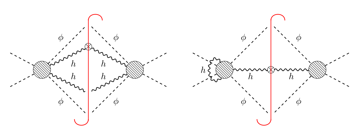
Figure 3: The picture shows how the cancellation of infrared divergences between real and virtual graviton emissions works for the gravitational energy event shape

Before looking at the classical limit, it is worth looking at how infrared divergences will cancel for the gravitational energy event shape in general. At order $G^{4}$ we have,

$$\left<\text{out}\right|\mathcal{\tilde{E}}_{\text{GR}}(\hat{\mathbf{n}})\left|\text{out}\right>\Big{|}_{\mathcal{O}(G^{4})}$$

$$=\int\widetilde{\mathrm{d}^{3}p_{3}}\int\widetilde{\mathrm{d}^{3}p_{4}}\sum_{\sigma_{1}=\pm 2}\int\widetilde{\mathrm{d}^{3}k_{1}}\,(2\pi)^{4}\delta^{4}\left(\sum_{i=1}^{4}\eta_{i}p_{i}+k_{1}\right)$$

$$\hskip 50.0pt\times\left[(E_{k_{1}})\delta^{2}(\Omega_{\mathbf{\hat{k}}_{1}}-\Omega_{\hat{\mathbf{n}}})\right]|\mathcal{A}^{\text{GR}}(p_{1},p_{2};p_{3},p_{4},\{k_{1},\sigma_{1}\})|^{2}$$

$$+\int\widetilde{\mathrm{d}^{3}p_{3}}\int\widetilde{\mathrm{d}^{3}p_{4}}\,\frac{1}{2}\sum_{\sigma_{1},\sigma_{2}=\pm 2}\int\widetilde{\mathrm{d}^{3}k_{1}}\int\widetilde{\mathrm{d}^{3}k_{2}}\,(2\pi)^{4}\delta^{4}\left(\sum_{i=1}^{4}\eta_{i}p_{i}+\sum_{l=1}^{2}k_{l}\right)$$

$$\hskip 50.0pt\times\left[\sum_{l=1}^{2}(E_{k_{l}})\delta^{2}(\Omega_{\mathbf{\hat{k}}_{l}}-\Omega_{\hat{\mathbf{n}}})\right]|\mathcal{A}^{\text{GR}}(p_{1},p_{2};p_{3},p_{4},\{k_{1},\sigma_{1}\},\{k_{2},\sigma_{2}\})|^{2}.$$ (137)

The first contribution includes loop contributions related to virtual gravitons

$$|\mathcal{A}^{\text{GR}}(p_{1},p_{2};p_{3},p_{4},\{k_{1},\sigma_{1}\})|^{2}\Big{|}_{\mathcal{O}(G^{4})}=|\mathcal{A}^{\text{GR}}(p_{1},p_{2};p_{3},p_{4},\{k_{1},\sigma_{1}\})|^{2}\Big{|}_{\mathcal{O}(G^{3})}$$

$$\times\left[-\frac{G}{4\pi^{2}}\log\left(\frac{\Lambda}{\lambda}\right)\int\mathrm{d}\Omega_{\mathbf{\hat{k}}}\left(\sum_{i,j=1}^{4}\eta_{i}\eta_{j}\frac{2(p_{i}\cdot p_{j})^{2}-m_{i}^{2}m_{j}^{2}}{(E_{p_{i}}-\mathbf{p}_{i}\cdot\hat{\mathbf{k}})(E_{p_{j}}-\mathbf{p}_{j}\cdot\hat{\mathbf{k}})}\right)\right],$$ (138)

where we have regularized the integral with the ultraviolet cutoff $\Lambda$ Weinberg:1965nx . The second term instead has a divergent contribution which comes from the emission of one real graviton, since integrating over the 2-gravitons phase space gives

$$\frac{1}{2}\sum_{\sigma_{1},\sigma_{2}=\pm 2}\int_{\lambda}^{E_{\text{wave}}}\frac{\mathrm{d}E_{k_{1}}(E_{k_{1}})}{2(2\pi)^{3}}\int_{\lambda}^{E_{\text{wave}}}\frac{\mathrm{d}E_{k_{2}}(E_{k_{2}})}{2(2\pi)^{3}}\int\mathrm{d}\Omega_{\mathbf{\hat{k}}_{1}}\,\int\mathrm{d}\Omega_{\mathbf{\hat{k}}_{2}}\,\Theta(E_{\text{wave}}-E_{k_{1}}-E_{k_{2}})$$

$$\hskip 70.0pt\times\left[\sum_{l=1}^{2}(E_{k_{l}})\delta^{2}(\Omega_{\mathbf{\hat{k}}_{l}}-\Omega_{\hat{\mathbf{n}}})\right]\prod_{l=1}^{2}\Bigg{|}\sum_{i=1}^{4}\eta_{i}\frac{\kappa}{2}\frac{\epsilon^{\sigma_{l}}_{\mu\nu}(\mathbf{k}_{l})p_{i}^{\mu}p_{i}^{\nu}}{p_{i}\cdot k_{l}}\Bigg{|}^{2}$$

$$=G\frac{E_{\text{wave}}}{4\pi^{2}}\left(\sum_{i,j=1}^{4}\eta_{i}\eta_{j}\frac{2(p_{i}\cdot p_{j})^{2}-m_{i}^{2}m_{j}^{2}}{(E_{p_{i}}-\mathbf{p}_{i}\cdot\hat{\mathbf{n}})(E_{p_{j}}-\mathbf{p}_{j}\cdot\hat{\mathbf{n}})}\right)$$

$$\hskip 70.0pt\times\log\left(\frac{E_{\text{wave}}}{\lambda}\right)\frac{G}{4\pi^{2}}\left[\int\mathrm{d}\Omega_{\mathbf{\hat{k}}}\sum_{i,j=1}^{4}\eta_{i}\eta_{j}\frac{2(p_{i}\cdot p_{j})^{2}-m_{i}^{2}m_{j}^{2}}{(E_{p_{i}}-\mathbf{p}_{i}\cdot\hat{\mathbf{k}})(E_{p_{j}}-\mathbf{p}_{j}\cdot\hat{\mathbf{k}})}\right],$$ (139)

where we have used the fact that

$$\int_{\lambda}^{E_{\text{wave}}}\mathrm{d}E_{k_{1}}\,\int_{\lambda}^{E_{\text{wave}}}\mathrm{d}E_{k_{2}}\,\frac{1}{E_{k_{2}}}\Theta(E_{\text{wave}}-E_{k_{1}}-E_{k_{2}})\stackrel{{\scriptstyle E_{k_{1}},E_{k_{2}}\ll E_{\text{wave}}}}{{\simeq}}E_{\text{wave}}\log\left(\frac{E_{\text{wave}}}{\lambda}\right),$$ (140)

which is valid as long as we can neglect the single graviton energies (suppressed by $\hbar$) compared to the energy of the wave $E_{k_{1}},E_{k_{2}}\ll E_{\text{wave}}$, as noticed in Addazi:2019mjh .

One can then perform the regularized sum in (137)

$$\left<\text{out}\right|\mathcal{\tilde{E}}_{\text{GR}}(\hat{\mathbf{n}})\left|\text{out}\right>\Big{|}_{\mathcal{O}(G^{4})}=\int\mathrm{d}\Omega_{\mathbf{p}_{\text{CM}}}\frac{|\mathbf{p}_{\text{CM}}|}{16\pi^{2}\sqrt{s}}|\mathcal{A}^{\text{GR}}(p_{1},p_{2};p_{3},p_{4})|^{2}$$

$$\times G\frac{E_{\text{wave}}}{4\pi^{2}}\left(\sum_{i,j=1}^{4}\eta_{i}\eta_{j}\frac{2(p_{i}\cdot p_{j})^{2}-m_{i}^{2}m_{j}^{2}}{(E_{p_{i}}-\mathbf{p}_{i}\cdot\hat{\mathbf{n}})(E_{p_{j}}-\mathbf{p}_{j}\cdot\hat{\mathbf{n}})}\right)$$

$$\times\log\left(\frac{E_{\text{wave}}}{\Lambda}\right)\frac{G}{4\pi^{2}}\left[\int\mathrm{d}\Omega_{\mathbf{\hat{k}}}\sum_{i,j=1}^{4}\eta_{i}\eta_{j}\frac{2(p_{i}\cdot p_{j})^{2}-m_{i}^{2}m_{j}^{2}}{(E_{p_{i}}-\mathbf{p}_{i}\cdot\hat{\mathbf{k}})(E_{p_{j}}-\mathbf{p}_{j}\cdot\hat{\mathbf{k}})}\right],$$ (141)

which is infrared finite as expected. One can then repeat the same argument for the $G^{3+n}$-th order contribution

$$\left<\text{out}\right|\mathcal{E}_{\text{GR}}(\hat{\mathbf{n}})\left|\text{out}\right>\Big{|}_{\mathcal{O}(G^{3+n})}=\int\mathrm{d}\Omega_{\mathbf{p}_{\text{CM}}}\frac{|\mathbf{p}_{\text{CM}}|}{16\pi^{2}\sqrt{s}}|\mathcal{A}^{\text{GR}}(p_{1},p_{2};p_{3},p_{4})|^{2}$$

$$\times G\frac{E_{\text{wave}}}{4\pi^{2}}\left(\sum_{i,j=1}^{4}\eta_{i}\eta_{j}\frac{2(p_{i}\cdot p_{j})^{2}-m_{i}^{2}m_{j}^{2}}{(E_{p_{i}}-\mathbf{p}_{i}\cdot\hat{\mathbf{n}})(E_{p_{j}}-\mathbf{p}_{j}\cdot\hat{\mathbf{n}})}\right)$$

$$\times\sum_{M^{\prime}=0}^{n}\frac{1}{M^{\prime}!}\log\left(\frac{E_{\text{wave}}}{\Lambda}\right)^{M^{\prime}}\left[\frac{G}{4\pi^{2}}\int\mathrm{d}\Omega_{\mathbf{\hat{k}}}\sum_{i,j=1}^{4}\eta_{i}\eta_{j}\frac{2(p_{i}\cdot p_{j})^{2}-m_{i}^{2}m_{j}^{2}}{(E_{p_{i}}-\mathbf{p}_{i}\cdot\hat{\mathbf{k}})(E_{p_{j}}-\mathbf{p}_{j}\cdot\hat{\mathbf{k}})}\right]^{M^{\prime}},$$ (142)

where $M^{\prime}=M-1$.

It is worth noticing that this situation is in contrast with QCD case where the gluon energy event shape is infrared divergent and one has to sum also over quarks energy event shapes to get a well-defined (i.e. an infrared finite) answer Basham:1977iq . The cancellation of infrared divergences in this setting is similar to what was found for the graviton emission cross section by Donoghue Donoghue:1999qh .

7.2 The 2-points gravitational energy event shape

The main object of interest here will be

$$\left<\text{out}\right|\mathcal{\tilde{E}}(\hat{\mathbf{n}}_{1})\mathcal{\tilde{E}}^{\prime}(\hat{\mathbf{n}}_{2})\left|\text{out}\right>=\left<\text{in}\right|S^{\dagger}\mathcal{\tilde{E}}(\hat{\mathbf{n}}_{1})\mathcal{\tilde{E}}^{\prime}(\hat{\mathbf{n}}_{2})S\left|\text{in}\right>.$$ (143)

By inserting a completeness relation of on-shell final states $\sum_{X}\left|\mathbf{X}\right>\left<\mathbf{X}\right|$ between the two gravitational ANEC operators at infinity we get

$$\left<\text{out}\right|\mathcal{\tilde{E}}(\hat{\mathbf{n}}_{1})\mathcal{\tilde{E}}^{\prime}(\hat{\mathbf{n}}_{2})\left|\text{out}\right> =\sum_{X}\left<\text{in}\right|S^{\dagger}\mathcal{\tilde{E}}(\hat{\mathbf{n}}_{1})\left|\mathbf{X}\right>\left<\mathbf{X}\right|\mathcal{\tilde{E}}^{\prime}(\hat{\mathbf{n}}_{2})S\left|\text{in}\right>$$

$$=\sum_{X}w_{\mathcal{\tilde{E}}}(\hat{\mathbf{n}}_{1})w^{\prime}_{\mathcal{\tilde{E}}}(\hat{\mathbf{n}}_{2})|\left<\mathbf{X}\right|S\left|\text{in}\right>|^{2}.$$ (144)

In details

$$\left<\text{out}\right|\mathcal{\tilde{E}}_{\text{GR}}(\hat{\mathbf{n}}_{1})\mathcal{\tilde{E}}^{\prime}_{\text{GR}}(\hat{\mathbf{n}}_{2})\left|\text{out}\right>\Big{|}_{\mathcal{O}(G^{4})}$$

$$=\int\widetilde{\mathrm{d}^{3}p_{3}}\int\widetilde{\mathrm{d}^{3}p_{4}}\frac{1}{2}\sum_{\sigma_{1},\sigma_{2}=\pm 2}\int\widetilde{\mathrm{d}^{3}k_{1}}\int\widetilde{\mathrm{d}^{3}k_{2}}$$

$$\times\Big{[}(E_{k_{1}})(E_{k_{1}})\delta^{2}(\Omega_{\mathbf{\hat{k}}_{1}}-\Omega_{\hat{\mathbf{n}}_{1}})\delta^{2}(\Omega_{\mathbf{\hat{k}}_{1}}-\Omega_{\hat{\mathbf{n}}_{2}})+(E_{k_{2}})(E_{k_{2}})\delta^{2}(\Omega_{\mathbf{\hat{k}}_{2}}-\Omega_{\hat{\mathbf{n}}_{1}})\delta^{2}(\Omega_{\mathbf{\hat{k}}_{2}}-\Omega_{\hat{\mathbf{n}}_{2}})$$

$$\hskip 7.0pt+2(E_{k_{1}})(E_{k_{2}})\delta^{2}(\Omega_{\mathbf{\hat{k}}_{1}}-\Omega_{\hat{\mathbf{n}}_{1}})\delta^{2}(\Omega_{\mathbf{\hat{k}}_{2}}-\Omega_{\hat{\mathbf{n}}_{2}})\Big{]}|\left<\{\mathbf{k}_{1},\sigma_{1}\}\{\mathbf{k}_{2},\sigma_{2}\}\mathbf{p}_{3}\mathbf{p}_{4}\right|S\left|\mathbf{p}_{1}\mathbf{p}_{2}\right>|^{2}.$$ (145)

Contrary to the 1-pt energy event shape, here we get also contact terms which correspond to the case where the two detectors are aligned along the same direction. These terms are usually included in QCD energy event shapes and they are required in order to remove collinear divergences Basham:1978bw , but classical gravity does not have such type of collinear divergences Akhoury:2011kq . We will thus restrict our attention to the generic case $\hat{\mathbf{n}}_{1}\neq\hat{\mathbf{n}}_{2}$:

$$\left<\text{out}\right|\mathcal{\tilde{E}}_{\text{GR}}(\hat{\mathbf{n}}_{1})\mathcal{\tilde{E}}^{\prime}_{\text{GR}}(\hat{\mathbf{n}}_{2})\left|\text{out}\right>\Big{|}_{\mathcal{O}(G^{4})}=\int\widetilde{\mathrm{d}^{3}p_{3}}\int\widetilde{\mathrm{d}^{3}p_{4}}\,\frac{1}{2}\sum_{\sigma_{1},\sigma_{2}=\pm 2}\int\widetilde{\mathrm{d}^{3}k_{1}}\int\widetilde{\mathrm{d}^{3}k_{2}}$$

$$\hskip 50.0pt\times(2E_{k_{1}}E_{k_{2}}\delta^{2}(\Omega_{\mathbf{\hat{k}}_{1}}-\Omega_{\hat{\mathbf{n}}_{1}})\delta^{2}(\Omega_{\mathbf{\hat{k}}_{2}}-\Omega_{\hat{\mathbf{n}}_{2}}))|\left<\{\mathbf{k}_{1},\sigma_{1}\}\{\mathbf{k}_{2},\sigma_{2}\}\mathbf{p}_{3}\mathbf{p}_{4}\right|S\left|\mathbf{p}_{1}\mathbf{p}_{2}\right>|^{2}.$$ (146)

At this point we can repeat the integration as we did before to get

$$\left<\text{out}\right|\mathcal{\tilde{E}}_{\text{GR}}(\hat{\mathbf{n}}_{1})\mathcal{\tilde{E}}^{\prime}_{\text{GR}}(\hat{\mathbf{n}}_{2})\left|\text{out}\right>\Big{|}_{\mathcal{O}(G^{4})}=\int\mathrm{d}\Omega_{\mathbf{p}_{\text{CM}}}\frac{|\mathbf{p}_{\text{CM}}|}{16\pi^{2}\sqrt{s}}|\mathcal{A}^{\text{GR}}(p_{1},p_{2};p_{3},p_{4})|^{2}$$

$$\hskip 60.0pt\times\prod_{l=1}^{2}\left[G\frac{E_{\text{wave}}}{4\pi^{2}}\left(\sum_{i,j=1}^{4}\eta_{i}\eta_{j}\frac{2(p_{i}\cdot p_{j})^{2}-m_{i}^{2}m_{j}^{2}}{(E_{p_{i}}-\mathbf{p}_{i}\cdot\hat{\mathbf{n}}_{l})(E_{p_{j}}-\mathbf{p}_{j}\cdot\hat{\mathbf{n}}_{l})}\right)\right].$$ (147)

As we can see, despite being a natural quantum observable the 2-point gravitational energy event shape factorizes, i.e. there is no degree of correlation between the two emissions. This is due to the soft limit we are considering and ultimately related to the coherent state structure of the radiation Ciafaloni:2018uwe . It would be very interesting to compute the non-trivial (connected) 2-point energy event shape in a quantum theory of gravity from the six point amplitude with 4 massive scalars and 2 gravitons, which should provide the leading infrared finite contribution to this observable.

7.3 Gravitational wave energy event shapes and classical factorization

So far we have discussed the quantum picture, where energy event shape correlators are a non-trivial infrared-safe prediction. For our problem in the classical soft limit, as we will see, only the 1-point event shape will be non-trivial because of factorization properties. Let’s first discuss how to achieve the classical limit. We are interested in the limit where those gravitons contribute coherently to a (suitably localized) wave travelling in a specific direction. To make this precise, one can study the interaction hamiltonian for our theory of scalars minimally coupled with gravity in the linearized gravity approximation and in asymptotic limit $|t|\to+\infty$ Ware:2013zja

$$H(t) =H_{0}+V^{\text{asy}}(t)=H_{0}-\int\mathrm{d}^{3}x\,h^{\mu\nu}(t,\mathbf{x})T^{\text{asy}}_{\mu\nu}(t,\mathbf{x}),$$

$$T^{\text{asy}}_{\mu\nu} =\sum_{i=1,2}\frac{\kappa}{2}\int\widetilde{\mathrm{d}^{3}p}\,\frac{p^{\mu}p^{\nu}}{E_{p}}\rho_{i}(\mathbf{p})\delta^{3}\left(\mathbf{x}-t\frac{\mathbf{p}}{E_{p}}\right),$$ (148)

where $H_{0}$ is the free hamiltonian, $\rho_{i}(\mathbf{p})=b^{\dagger}_{i}(\mathbf{p})b_{i}(\mathbf{p})$ is the number operator for the $i$-th scalar field and $(t,\mathbf{x})$ are the coordinates of the asymptotic trajectory of the scalar particles. This result is is valid only at first order in the perturbation $h_{\mu\nu}$, but it tells something important about the asymptotic dynamics: solving the asymptotic Schrödinger equation for the potential $V^{\text{asy}}(t)$ gives an evolution operator which generates an infinite number of (soft) gravitons, or more precisely a coherent state of gravitons

$$\left|\{\alpha_{p},\sigma\}\right>=N_{\alpha}\exp\left[\int\widetilde{\mathrm{d}^{3}p}\left(\alpha_{p}(\mathbf{p})a^{\dagger}_{\sigma}(\mathbf{p})-\mathrm{h.c.}\right)\right]\left|0\right>$$ (149)

for a suitable function $\alpha_{p}(\mathbf{p})$ related to the structure of the asymptotic stress momentum tensor of the scalar particle $T^{\text{asy}}_{\mu\nu}$. In this specific context the state (149) is referred as Faddeev-Kulish state Kulish:1970ut . This gives an insight about how the quantum scattering theory generates a classical gravitational wave, composed of infinitely many gravitons, at least in the soft kinematic regime. More details about the connection of coherent states with the classical limit will be provided in Cristofoli:2021vyo .

In our case we can take the sum over all contributions $M=1,..,+\infty$, which implies to sum over $M^{\prime}=0,..,+\infty$ in our expression for the gravitational wave event shape in (142):

$$\left<\text{out}\right|\mathcal{\tilde{E}}_{\text{GR}}(\hat{\mathbf{n}})\left|\text{out}\right>\Big{|}_{\text{class}}=G\frac{E_{\text{wave}}}{4\pi^{2}}\int\mathrm{d}\Omega_{\mathbf{p}_{\text{CM}}}\frac{|\mathbf{p}_{\text{CM}}|}{16\pi^{2}\sqrt{s}}|\mathcal{A}^{\text{GR}}(p_{1},p_{2};p_{3},p_{4})|^{2}$$

$$\times\left(\sum_{i,j=1}^{4}\eta_{i}\eta_{j}\frac{2(p_{i}\cdot p_{j})^{2}-m_{i}^{2}m_{j}^{2}}{(E_{p_{i}}-\mathbf{p}_{i}\cdot\hat{\mathbf{n}})(E_{p_{j}}-\mathbf{p}_{j}\cdot\hat{\mathbf{n}})}\right)\left(\frac{E_{\text{wave}}}{\Lambda}\right)^{\frac{G}{2\pi}\sum_{i,j}\eta_{i}\eta_{j}\frac{m_{i}m_{j}(1+\beta^{2}_{ij})}{\beta_{ij}(1-\beta^{2}_{ij})^{\frac{1}{2}}}\log\left(\frac{1+\beta_{ij}}{1-\beta_{ij}}\right)},$$ (150)

where $\beta_{ij}=\sqrt{1-\frac{m_{i}^{2}m_{j}^{2}}{(p_{i}\cdot p_{j})^{2}}}$. This is consistent with the graviton production rate in Weinberg Weinberg:1965nx under our hypotheses. Once normalized by the total cross section we have

$$\Big{\langle}\mathcal{\tilde{E}}_{\text{GR}}(\hat{\mathbf{n}})\Big{\rangle}\Big{|}_{\text{class}}=\frac{E_{\text{wave}}G}{4\pi^{2}}\left(\sum_{i,j=1}^{4}\eta_{i}\eta_{j}\frac{2(p_{i}\cdot p_{j})^{2}-m_{i}^{2}m_{j}^{2}}{(E_{p_{i}}-\mathbf{p}_{i}\cdot\hat{\mathbf{n}})(E_{p_{j}}-\mathbf{p}_{j}\cdot\hat{\mathbf{n}})}\right)$$

$$\hskip 160.0pt\times\left(\frac{E_{\text{wave}}}{\Lambda}\right)^{\frac{G}{2\pi}\sum_{i,j}\eta_{i}\eta_{j}\frac{m_{i}m_{j}(1+\beta^{2}_{ij})}{\beta_{ij}(1-\beta^{2}_{ij})^{\frac{1}{2}}}\log\left(\frac{1+\beta_{ij}}{1-\beta_{ij}}\right)}$$ (151)

and if we try to compute the gravitational energy-energy correlator at the classical level

$$\Big{\langle}\mathcal{\tilde{E}}_{\text{GR}}(\hat{\mathbf{n}}_{1})\mathcal{\tilde{E}}^{\prime}_{\text{GR}}(\hat{\mathbf{n}}_{2}))\Big{\rangle}\Big{|}_{\text{class}}=\Big{\langle}\mathcal{\tilde{E}}_{\text{GR}}(\hat{\mathbf{n}}_{1})\Big{\rangle}\Big{|}_{\text{class}}\Big{\langle}\mathcal{\tilde{E}}^{\prime}_{\text{GR}}(\hat{\mathbf{n}}_{2})\Big{\rangle}\Big{|}_{\text{class}},$$ (152)

which is a consequence of the classical (soft) factorization. This can be shown explicitly using the coherent state in (149).

7.4 Infrared safety of gravitational energy event shapes and soft BMS supertranslation

It is possible to do an interesting consistency check about infrared safety of the gravitational energy event shapes by looking at how soft supertranslation symmetry affects such matrix elements. Earlier we have used an infrared cutoff and we have observed the cancellation of infrared divergences as in the Bloch-Nordsieck mechanism, but it would be nice to understand if there is a theoretical reason for these event shapes to be infrared finite.

It is well known that the action of the soft supertranslation mode corresponds to an insertion of a soft graviton at the level of S-matrix elements Strominger:2013jfa ; He:2014laa . In particular the generator of such symmetry reads

$$T_{\text{soft}}(f) =\frac{1}{16\pi G}\int\mathrm{d}^{2}\zeta\left[\partial_{\zeta}D^{\bar{\zeta}}C_{\bar{\zeta}\bar{\zeta}}+\partial_{\bar{\zeta}}D^{\zeta}C_{\zeta\zeta}\right]f(\zeta,\bar{\zeta})$$

$$=\lim_{E\to 0}\frac{E}{4\pi\kappa}\int\mathrm{d}^{2}\zeta\,\left[(a_{+}(E\hat{\mathbf{n}})+a^{\dagger}_{-}(E\hat{\mathbf{n}}))D_{\bar{\zeta}}^{2}f+h.c.\right],$$ (153)

where $f(\zeta,\bar{\zeta})$ is an arbitrary function on the celestial sphere. Its action on graviton creation operators is given by

$$[T_{\text{soft}}(f),a_{+}(\mathbf{k})]=\frac{8\pi^{2}}{\kappa}\frac{\delta(E_{k})}{\gamma_{\zeta_{k}\bar{\zeta}_{k}}}D^{2}_{\zeta}f\,,\qquad[T_{\text{soft}}(f),a_{-}(\mathbf{k})]=\frac{8\pi^{2}}{\kappa}\frac{\delta(E_{k})}{\gamma_{\zeta_{k}\bar{\zeta}_{k}}}D^{2}_{\bar{\zeta}}f,$$ (154)

and the one with creation operators is fixed because $T_{\text{soft}}(f)$ is hermitian. The latter implies that

$$[T_{\text{soft}}(f),a^{\dagger}_{\sigma}(\mathbf{k})]^{\dagger}=-[T_{\text{soft}}(f),a_{\sigma}(\mathbf{k})]\qquad\forall\,\sigma=\pm 2.$$ (155)

We now consider a gravitational event shape of the form

$$\left<\text{out}\right|\mathcal{\tilde{P}}_{\mu,\text{GR}}(\hat{\mathbf{n}})\left|\text{out}\right>=\sum_{X}\left<\text{in}\right|S^{\dagger}\mathcal{\tilde{P}}_{\mu,\text{GR}}(\hat{\mathbf{n}})\left|\mathbf{X}\right>\left<\mathbf{X}\right|S\left|\text{in}\right>$$ (156)

and we want to check whether this definition is invariant or not under BMS soft supertranslations, i.e. under the addition of a soft graviton. If it is, this provides a strong evidence that (156) is actually infrared finite, i.e. insensitive to soft (graviton) physics. A short calculation shows that

$$[T_{\text{soft}}(f),\mathcal{\tilde{P}}_{\mu,\text{GR}}(\hat{\mathbf{n}})]=\frac{n_{\mu}}{2\pi\kappa\gamma_{\zeta_{\hat{\mathbf{n}}}\bar{\zeta}_{\hat{\mathbf{n}}}}}\lim_{E_{p}\to 0}(E_{p})^{2}\left[D^{2}_{\zeta}f\,a^{\dagger}_{+}(E_{p}\hat{\mathbf{n}})+D^{2}_{\bar{\zeta}}f\,a^{\dagger}_{-}(E_{p}\hat{\mathbf{n}})-h.c.\right]$$ (157)

and since the addition of a soft graviton gives the usual Weinberg soft factor with a pole in $E_{p}$, the action (157) annihilates every S-matrix element (once we insert the completeness relation) He:2014laa .

It would be interesting to understand in more details if the invariance under the soft modes of large gauge symmetries, BMS supertranslations and in general asymptotic symmetries of massless particles always guarantees the IR-finiteness (in the soft sense) of a matrix element in a QFT. This could be helpful to prove in general whether for other on-shell observables, for example like the ones defined in Kosower:2018adc , infrared divergences are always going to cancel.

8 Discussion and Conclusions

Einstein equations solved near null infinity and BMS balance laws are of particular relevance for studying the property of the radiation at infinity, like its energy and its angular momentum which are captured by detectors localized at spatial infinity in a particular direction $\mathbf{n}$. Once we integrate Einstein equations over the retarded time, say in Bondi gauge, new non-local operators appear which are commonly called light-ray operators. For our definition of light-ray operators, we integrate over the entire retarded time interval $u\in\mathbb{R}$, which allows us to extract a suitable notion of density of energy and angular momentum flux produced during a scattering event. This is the natural framework where contributions coming from different massless particles combine together in a single expression.

Besides the direct physical applications, the algebra of such non-local light-ray operators at infinity is of intrinsic interest since it can be considered some sort of “detector algebra”. In the conformal case the algebra was clarified in a beautiful work by Cordova and Shao Cordova:2018ygx where they took advantage of the Hofman-Maldacena map Hofman:2008ar to move the light-sheet at infinity to a finite distance and they analized the structure of the algebra based on pure symmetry arguments. Therefore, it is of particular relevance to understand such algebra in the case of physical theories (possibly non-conformal) in 4 dimensions, which is the main purpose of this work.

Here we interpret the insertion of light-ray operators in a correlation function as the insertion of a physical detector which is capturing properties of the distribution of outgoing particles at null infinity and we work in perturbation theory. In particular, we focus on the case of massless particles with integer spin and we use the saddle point estimate for the leading contribution to the stress tensor components. This provides an explicit representation of the hard mode contributions to light-ray operators, which is of particular relevance for physical detectors which have any kind of lower energy resolution. The structure we find is consistent with the quantum fields localizing on point-particle trajectory, since the stress tensor expression reduces to the pointlike one, possibly with the spin contribution Pasterski:2015tva . The universality of these expressions seems to point to some universality of light-ray operators in 4 dimensions beyond the conformal case. While a more rigorous analysis would be desired for the $[\mathcal{N}_{z}(\hat{\mathbf{n}}_{1}),\mathcal{N}_{\bar{z}}(\hat{\mathbf{n}}_{2})]$ commutator, our results are consistent with the algebra of Cordova and Shao Cordova:2018ygx . For the spin 1 case coupled with matter, an interaction term coming from the mixing of the so-called radiative and coulombic modes Ashtekar:2017wgq ; Ashtekar:2017ydh seems to break the algebra.

There could be extensions of the algebra in the soft sector for the angular momentum flux, in particular in the non-abelian case where we have observed a non-trivial boundary contribution whose insertion is related to the soft gluon theorem. This would required a detailed analysis of the Hilbert space factorization into soft and hard modes, which is beyond the scope of the paper He:2020ifr . More generally it would be interesting to establish a basis of non-local operators at null infinity, making contact also with integrals of current operators along the retarded time and to Wilson line operators. It would be also nice to have a full analysis of the algebra in the Bondi gauge, for example by using Newman-Penrose techniques Newman:1961qr ; Frolov:1977bp .

Borrowing some ideas from the QCD event shape detector operators, we have defined a suitable notion of energy event shape in the gravitational case using the Bondi news squared operator. Working with an EFT of gravity in the classical limit, we study the gravitational radiation produced in a particular direction $\hat{\mathbf{n}}$ in the sky from the scattering of compact objects in the leading soft approximation. In this simple limit, the Glauber-Sudarshan representation Glauber:1963tx ; Sudarshan:1963ts of the QFT radiation density matrix reduces to a single coherent state and we can sum up all graviton contributions to get the classical result which matches the literature on the zero frequency limit (ZFL) Smarr:1977fy ; Addazi:2019mjh . Working in the approximation where we neglect the single graviton energies compared to the energy of the wave, we observe that there is a cancellation of infrared divergences for the gravitational energy event shape which gives an infrared finite result. It would be interesting to extend our analysis to include classical corrections to our result due to additional finite energy contributions and outside the zero frequency limit, as done in Gruzinov:2014moa ; Addazi:2019mjh for the soft gravitational radiation. In the classical limit, the correlation function of gravitational energy event shapes factorize because the graviton emissions are uncorrelated, which is in agreement with the single coherent state structure. In particular we have defined also the 2-point gravitational energy correlator, which is particularly interesting especially outside the soft classical limit where non-trivial contributions should come into play. Since it should be a non-trivial infrared safe prediction of quantum gravity, it would be very fascinating to explore this further. Interestingly, recently it was pointed out that a signature of the quantum state of gravitons might be observable especially if it deviates from the coherent state prediction Parikh:2020nrd ; Parikh:2020kfh ; Parikh:2020fhy .

Acknowledgements We would like to thank Aron Wall, Simon Caron-Huot, Donal O’Connell, Manuel Accettulli-Huber and Tristan McLoughlin for useful discussions. We thank in particular Simon Caron-Huot for stimulating discussions at different stages of the project and for comments on the draft. R.G. would like to thank A.Cristofoli, D.Kosower and D.O’Connell for many discussions on a related project. This project has received funding from the European Union’s Horizon 2020 research and innovation programme under the Marie Skłodowska-Curie grant agreement No. 764850. A.P. is grateful for funds provided by the Fonds de Recherche du Québec.

Appendix A Notations

The signature of the spacetime is mostly minus $(+,-,-,-)$. We have set $\hbar=c=1$.

Appendix B Detector light-cone definition of $\mathcal{\tilde{E}}(\hat{\mathbf{n}})$ and $\mathcal{\tilde{K}}(\hat{\mathbf{n}})$ light-ray operators

To connect our discussion to the usual QCD event shape literature and in order to indroduce a more covariant formalism, we identify a detector by its set of coordinates $x^{\mu}=(t,r\hat{\mathbf{n}})=\left(x_{-}n^{\mu}+x_{+}\bar{n}^{\mu}\right)$ where

$$x_{+} =\frac{t-r}{2}=\frac{(x\cdot n)}{(n\cdot\bar{n})}\qquad x_{-}=\frac{t+r}{2}=\frac{(x\cdot\bar{n})}{(n\cdot\bar{n})},$$

$$n^{\mu} =(1,\hat{\mathbf{n}})\qquad\bar{n}^{\mu}=(1,-\hat{\mathbf{n}})\qquad n^{2}=\bar{n}^{2}=0.$$ (158)

We can complete the basis with two spacelike vectors $m_{A}$ which satisfy

$$x_{A} =\frac{(x\cdot m_{A})}{(m_{A}\cdot m_{A})}\qquad m_{A}\cdot n=m_{A}\cdot\bar{n}=0\qquad m_{A}\cdot m_{B}=-\delta_{AB}\qquad\forall\,A\in\{1,2\},$$ (159)

so that a generic point in spacetime is uniquely identified as $x^{\mu}=x_{-}n^{\mu}+x_{+}\bar{n}^{\mu}+x_{A}m_{A}^{\mu}$. The completeness relation reads

$$\eta_{\mu\nu}=\frac{n_{\mu}\bar{n}_{\nu}+\bar{n}_{\mu}n_{\nu}}{(n\cdot\bar{n})}+\frac{(m_{A})_{\mu}(m_{A})_{\nu}}{(m_{A}\cdot m_{A})},$$ (160)

which implies that $x\cdot y=2(x_{-}y_{+}+x_{+}y_{-})-x_{A}y_{A}$ and that the flat metric can be written as $\mathrm{d}s^{2}=\mathrm{d}x^{+}\mathrm{d}x^{-}-\mathrm{d}x^{A}\mathrm{d}x^{A}$. It is worth pointing out that since we are interested in the algebra of different detectors it makes more sense to use a system of coordinates adapted at null infinity, as we did in the main text. Moreover, the latter extends to the more general case of asymptotically flat geometries and that is crucial for physical applications.

We can write the ANEC operator at infinity in a covariant form as

$$\mathcal{\tilde{E}}(\hat{\mathbf{n}})=(n\cdot\bar{n})\int_{-\infty}^{+\infty}\mathrm{d}x_{+}\,\lim_{x_{-}\to\infty}(x_{-})^{2}T_{--}(x_{-}n+x_{+}\bar{n}),$$ (161)

where we have defined a covariant light-cone projection $T_{--}=\frac{\bar{n}^{\mu}\bar{n}^{\nu}}{(n\cdot\bar{n})^{2}}T_{\mu\nu}$. This expression is Lorentz covariant under rescalings of the type

$$n\to\rho\,n\qquad\bar{n}\to\rho\,\bar{n}$$ (162)

and it has weight $-3$. It is important to stress that for external non-localized states, like momentum eigenstates, we need to take the large $x_{-}$ limit first and then perform the integral as done in (161). The opposite is usually done in CFT for localized states, for which all notions are equivalent Hofman:2008ar ; Belitsky:2013xxa . In a similar way, we can write the momentum flow operator in a Lorentz covariant form as

$$\mathcal{\tilde{P}}_{\mu}(\hat{\mathbf{n}})=(n\cdot\bar{n})\int_{-\infty}^{+\infty}\mathrm{d}x_{+}\,\lim_{x_{-}\to\infty}(x_{-})^{2}T_{-\mu}(x_{-}n+x_{+}\bar{n}).$$ (163)

The next operator which we want to define is $\mathcal{\tilde{K}}(\hat{\mathbf{n}})$

$$\mathcal{\tilde{K}}(\hat{\mathbf{n}}) :=(n\cdot\bar{n})^{2}\int_{-\infty}^{+\infty}\mathrm{d}x_{+}(x_{+})\,\lim_{x_{-}\to\infty}(x_{-})^{2}T_{--}(x_{-}n+x_{+}\bar{n}),$$ (164)

which has weight $-2$. The formulation of the operator $\mathcal{\tilde{N}}_{A}(\hat{\mathbf{n}})$, where the index $A$ has to be interpreted as a projection over the transverse direction $m_{A}$ ($\mathcal{\tilde{N}}_{A}(\hat{\mathbf{n}})=\frac{(m_{A})^{\mu}\mathcal{\tilde{N}}_{\mu}(\hat{\mathbf{n}})}{(m_{A}\cdot m_{A})}$), is more difficult. This is related to the fact that one needs to rescale the index $A$ with $x_{-}$ to have a well-defined limit at infinity (see the related section 6.4).

Appendix C Light-ray operators for a light-sheet in the bulk

In the general, one would like to generalize the light-ray operator definition to allow them to be localized on general light-sheets in the bulk of the spacetime. If the theory is scale invariant (i.e. for all CFT for example) then the two definitions will coincide (see the explicit Hofman-Maldacena conformal transformation Hofman:2008ar ) but in general they will be different. To simplify our calculations, we can define

$$\tilde{x}_{-}:=\frac{x^{0}+x^{3}}{2}\qquad\tilde{x}_{+}:=\frac{x^{0}-x^{3}}{2},$$ (165)

so that light-sheets at fixed $\tilde{x}_{-}=\text{const}$ will be parametrized by the coordinate $\tilde{x}_{+}$. It is worth noticing that as $\tilde{x}_{-}\to+\infty$ we will have $\tilde{x}_{\pm}\to x_{\pm}$, so that there is no ambiguity with the previous notation in appendix B. For the light-sheet defined by $\tilde{x}_{-}=c$ with $c\in\mathbb{R}$, we define the light-ray family as

$$\mathcal{E}(\tilde{x}_{\perp}) :=\int_{-\infty}^{+\infty}\mathrm{d}\tilde{x}_{+}\,T_{--}(\tilde{x}_{+}=c,\tilde{x}_{-},\tilde{x}_{\perp}),$$

$$\mathcal{K}(\tilde{x}_{\perp}) :=\int_{-\infty}^{+\infty}\mathrm{d}\tilde{x}_{+}\,(\tilde{x}_{+})\,T_{--}(\tilde{x}_{+}=c,\tilde{x}_{-},\tilde{x}_{\perp}),$$

$$\mathcal{N}_{A}(\tilde{x}_{\perp}) :=(\partial_{A}\tilde{x}^{\mu})\int_{-\infty}^{+\infty}\mathrm{d}\tilde{x}_{+}T_{-\mu}(\tilde{x}_{+}=c,\tilde{x}_{-},\tilde{x}_{\perp}).$$ (166)

C.1 Spin 0

For a general light-sheet $c\in\mathbb{R}$ one needs to compute

$$T_{--}(x) =\frac{1}{4}\left(T_{00}(x)+T_{33}(x)-2T_{03}(x)\right)=\frac{1}{4}\left(\partial_{0}\phi(x)-\partial_{3}\phi(x)\right)^{2}=\partial_{-}\phi(x)\partial_{-}\phi(x),$$

$$T_{1-}(x) =\frac{1}{2}\left(T_{10}(x)-T_{13}(x)\right)=\frac{1}{2}\partial_{1}\phi(x)\left(\partial_{0}\phi(x)-\partial_{3}\phi(x)\right)=\partial_{1}\phi(x)\partial_{-}\phi(x),$$

$$T_{2-}(x) =\frac{1}{2}\left(T_{20}(x)-T_{23}(x)\right)=\frac{1}{2}\partial_{2}\phi(x)\left(\partial_{0}\phi(x)-\partial_{3}\phi(x)\right)=\partial_{2}\phi(x)\partial_{-}\phi(x).$$ (167)

The light-ray operators are then defined as

$$\mathcal{E}_{\text{scalar}}(\tilde{x}_{\perp}) :=\int_{-\infty}^{+\infty}\mathrm{d}\tilde{x}_{+}\,\partial_{-}\phi(\tilde{x})\partial_{-}\phi(\tilde{x})\Big{|}_{\tilde{x}_{-}=c},$$

$$\mathcal{N}_{A,\text{scalar}}(\tilde{x}_{\perp}) :=\int_{-\infty}^{+\infty}\mathrm{d}\tilde{x}_{+}\,\partial_{A}\phi(\tilde{x})\partial_{-}\phi(\tilde{x})\Big{|}_{\tilde{x}_{-}=c},$$

$$\mathcal{K}_{\text{scalar}}(\tilde{x}_{\perp}) :=\int_{-\infty}^{+\infty}\mathrm{d}\tilde{x}_{+}\,\tilde{x}_{+}\,\partial_{-}\phi(\tilde{x})\partial_{-}\phi(\tilde{x})\Big{|}_{\tilde{x}_{-}=c}.$$ (168)

It is quite remarkable that interactions drop out completely. This generically happens for scalar theories without derivative couplings and it implies some universality of the scalar light-ray algebra.

C.2 Spin 1

We have

$$T_{--} =\frac{1}{2}\eta^{ij}\left[(F_{0i}^{a}-F_{3i}^{a})(F_{j0}^{b}-F_{j3}^{b})\right]\text{Tr}(T^{a}T^{b})=(\partial_{-}A_{1}^{a})(\partial_{-}A_{1}^{a})+(\partial_{-}A_{2}^{a})(\partial_{-}A_{2}^{a}),$$

$$T_{1-} =F^{a}_{1\beta}\eta^{\alpha\beta}(F_{\alpha 0}^{b}-F_{\alpha 3}^{b})\text{Tr}(T^{a}T^{b})=(2\partial_{[1}A_{2]}^{a}+gf^{acd}A_{1}^{c}A_{2}^{d})(\partial_{-}A_{2}^{a})+2(\partial_{-}A^{a}_{+})(\partial_{-}A^{a}_{1}),$$

$$T_{2-} =F^{a}_{2\beta}\eta^{\alpha\beta}(F_{\alpha 0}^{b}-F_{\alpha 3}^{b})\text{Tr}(T^{a}T^{b})=(2\partial_{[2}A_{1]}^{a}+gf^{acd}A_{2}^{c}A_{1}^{d})(\partial_{-}A_{1}^{a})+2(\partial_{-}A^{a}_{+})(\partial_{-}A^{a}_{2}),$$ (169)

where in the last line have imposed the light-cone gauge

$$A_{0}=A_{3}\Leftrightarrow A_{-}=0.$$ (170)

We see that while $T_{--}(\tilde{x})$ is interaction independent in this gauge, $T_{A-}(\tilde{x})$ is not. Nevertheless, we are interested in light-ray operators where we integrate over the light-cone time $\tilde{x}_{+}$ and therefore we can take advantage of the equations of motion

$$\mathcal{D}_{\mu}F^{\mu,a}_{\,\,\,-}=\partial_{-}\left[\partial_{1}A_{1}^{a}+\partial_{2}A_{2}^{a}-2\partial_{-}A_{+}^{a}\right]+gf^{abc}(A_{1}^{b}\partial_{-}A_{1}^{c}+A_{2}^{b}\partial_{-}A_{2}^{c})=0,$$ (171)

provided that we take into account possible boundary terms at $\tilde{x}_{+}\to\pm\infty$. To fix completely the gauge for the boundary contributions, we can enforce the radiation gauge where together with the light-cone condition $A_{-}=0$ we have

$$\nabla^{\mu}A_{\mu}^{a}(x)\Big{|}_{\mathcal{I}^{-}}=\lim_{\tilde{x}_{+}\to-\infty}\left[2\partial_{-}A_{+}^{a}-\partial_{1}A_{1}^{a}-\partial_{2}A_{2}^{a}\right]=0,$$ (172)

thanks to which

$$\int_{-\infty}^{+\infty}\mathrm{d}\tilde{x}_{+}\,T_{1-}(\tilde{x}) =\int_{-\infty}^{+\infty}\mathrm{d}\tilde{x}_{+}\,\left[(\partial_{1}A_{2}^{a}-\partial_{2}A_{1}^{a})(\partial_{-}A_{2}^{a})+(\partial_{1}A_{1}^{a}+\partial_{2}A_{2}^{a})(\partial_{-}A_{1}^{a})\right]$$

$$+\frac{1}{2}A_{1}^{a}\left[2\partial_{-}A_{+}^{a}-\partial_{1}A_{1}^{a}-\partial_{2}A_{2}^{a}\right]_{\tilde{x}_{+}\to+\infty},$$

$$\int_{-\infty}^{+\infty}\mathrm{d}\tilde{x}_{+}\,T_{2-}(\tilde{x}) =\int_{-\infty}^{+\infty}\mathrm{d}\tilde{x}_{+}\,\left[(\partial_{2}A_{1}^{a}-\partial_{1}A_{2}^{a})(\partial_{-}A_{1}^{a})+(\partial_{1}A_{1}^{a}+\partial_{2}A_{2}^{a})(\partial_{-}A_{2}^{a})\right]$$

$$+\frac{1}{2}A_{2}^{a}\left[2\partial_{-}A_{+}^{a}-\partial_{1}A_{1}^{a}-\partial_{2}A_{2}^{a}\right]_{\tilde{x}_{+}\to+\infty}.$$ (173)

The light-ray operators are then defined as

$$\mathcal{E}_{\text{gluon}}(\tilde{x}_{\perp}) :=\sum_{i=1}^{2}\int_{-\infty}^{+\infty}\mathrm{d}\tilde{x}_{+}\,\partial_{-}A_{i}^{a}(\tilde{x})\partial_{-}A_{i}^{a}(\tilde{x})\Big{|}_{\tilde{x}_{-}=c},$$

$$\mathcal{K}_{\text{gluon}}(\tilde{x}_{\perp}) :=\sum_{i=1}^{2}\int_{-\infty}^{+\infty}\mathrm{d}\tilde{x}_{+}\,\tilde{x}_{+}\,\partial_{-}A_{i}^{a}(\tilde{x})\partial_{-}A_{i}^{a}(\tilde{x})\Big{|}_{\tilde{x}_{-}=c},$$

$$\mathcal{N}_{1,\text{gluon}}(\tilde{x}_{\perp}) :=\int_{-\infty}^{+\infty}\mathrm{d}\tilde{x}_{+}\,\left[(\partial_{1}A_{2}^{a}-\partial_{2}A_{1}^{a})(\partial_{-}A_{2}^{a})+(\partial_{1}A_{1}^{a}+\partial_{2}A_{2}^{a})(\partial_{-}A_{1}^{a})\right]\Big{|}_{\tilde{x}_{-}=c}$$

$$+\frac{1}{2}A_{1}^{a}\left[2\partial_{-}A_{+}^{a}-\partial_{1}A_{1}^{a}-\partial_{2}A_{2}^{a}\right]_{\tilde{x}_{+}\to+\infty},$$

$$\mathcal{N}_{2,\text{gluon}}(\tilde{x}_{\perp}) :=\int_{-\infty}^{+\infty}\mathrm{d}\tilde{x}_{+}\,\left[(\partial_{2}A_{1}^{a}-\partial_{1}A_{2}^{a})(\partial_{-}A_{1}^{a})+(\partial_{1}A_{1}^{a}+\partial_{2}A_{2}^{a})(\partial_{-}A_{2}^{a})\right]\Big{|}_{\tilde{x}_{-}=c}$$

$$+\frac{1}{2}A_{2}^{a}\left[2\partial_{-}A_{+}^{a}-\partial_{1}A_{1}^{a}-\partial_{2}A_{2}^{a}\right]_{\tilde{x}_{+}\to+\infty}.$$ (174)

If we compare to the self-interacting scalar case, we see that in YM theory interactions do not affect the definition of the operators $\mathcal{E}_{\text{gluon}}(\tilde{x}_{\perp})$ and $\mathcal{K}_{\text{gluon}}(\tilde{x}_{\perp})$ but they appear in $\mathcal{N}_{A,\text{gluon}}(\tilde{x}_{\perp})$ through the boundary contribution.

Appendix D Shear-inclusive ANEC and Raychaudhuri equation

The connection of the ANEC operator and its expectation value with causality properties of the underlying quantum field theory is well-known Hartman:2016lgu . A congruence of null (complete, achronal) geodesics obeys Raychaudhuri equation

$$\frac{\mathrm{d}\Theta}{\mathrm{d}\lambda}=-\frac{1}{2}\Theta^{2}-\sigma_{\mu\nu}\sigma^{\mu\nu}-8\pi GT^{\text{matter}}_{\mu\nu}k^{\mu}k^{\nu},$$ (175)

where $\lambda$ is the affine parameter, $\Theta=\frac{1}{A}\frac{\mathrm{d}A}{\mathrm{d}\lambda}$ is the expansion, $\sigma_{\mu\nu}$ is the shear and $k^{\mu}$ is a null vector of unit affine length which in our case we will take the light-sheet generator $k^{\mu}=\delta^{\mu}_{-}$. The right hand side of (175) immediately reminds us the enlarged definition of the matter ANEC with the gravitational contribution once we integrate along the null direction of the generator, albeit here (175) is purely classical in its nature. If we consider a generic congruence of null geodesics with starts at $\mathcal{I}^{-}$ and ends on $\mathcal{I}^{+}$, one can ask how the expansion parameter changes along the congruence. Classically, the ANEC condition $T^{\text{matter}}_{\mu\nu}k^{\mu}k^{\nu}\geq 0$ implies the classical focussing theorem, that is light-rays never “anti-focus” as long as matter has positive energy. Quantum mechanically, quantum fields can developed negative energy so that we generically need a quantum version of the ANEC Faulkner:2016mzt and of the focussing theorem Bousso:2015mna . In general, there are problems in including quantized gravity perturbations in this story. Nevertheless, assuming we have matter minimally coupled with gravity, for a stationary null surface one can quantize $h_{\mu\nu}$ on the null surface in light-front quantization Wall:2010cj and at the first order in the perturbation one can define a shear-inclusive ANEC operator of the form

$$\mathcal{E}_{\text{shear-inclusive}}=\int\mathrm{d}\lambda\left[\frac{1}{8\pi G}\sigma_{\mu\nu}\sigma^{\mu\nu}+T^{\text{matter}}_{\mu\nu}k^{\mu}k^{\nu}\right],$$ (176)

whose expectation value is positive definite $\langle\mathcal{E}^{\text{shear-inclusive}}\rangle\geq 0$ as it can be proved from the linearized Raychaudhuri equation Wall:2009wi . The connection to our previous definition of the shear-inclusive ANEC in the Bondi gauge consists in considering the asymptotically flat region for the geodesic congruence. Indeed in such region one can define a boundary shear as the limit of the rescaled shear of the congruence on future null infinity so that

$$\lim_{r\to+\infty}r^{2}\left[\frac{1}{8\pi G}\,\sigma_{\mu\nu}\sigma^{\mu\nu}+T^{\text{matter}}_{\mu\nu}k^{\mu}k^{\nu}\right]\sim\frac{1}{32\pi G}N_{\zeta\zeta}N^{\zeta\zeta}+\lim_{r\to\infty}r^{2}T^{\text{matter}}_{vv},$$ (177)

as proved in Bousso:2016vlt ; Bousso:2016wwu in order to study asymptotic entropy bounds.

References

- (1) C. L. Basham, L. S. Brown, S. Ellis and S. Love, Electron - Positron Annihilation Energy Pattern in Quantum Chromodynamics: Asymptotically Free Perturbation Theory, Phys. Rev. D 17 (1978) 2298.
- (2) C. Basham, L. S. Brown, S. D. Ellis and S. T. Love, Energy Correlations in electron - Positron Annihilation: Testing QCD, Phys. Rev. Lett. 41 (1978) 1585.
- (3) C. Basham, L. Brown, S. Ellis and S. Love, Energy Correlations in electron-Positron Annihilation in Quantum Chromodynamics: Asymptotically Free Perturbation Theory, Phys. Rev. D 19 (1979) 2018.
- (4) J. Ore, F.R. and G. F. Sterman, AN OPERATOR APPROACH TO WEIGHTED CROSS-SECTIONS, Nucl. Phys. B 165 (1980) 93.
- (5) N. Sveshnikov and F. Tkachov, Jets and quantum field theory, Phys. Lett. B 382 (1996) 403 [hep-ph/9512370].
- (6) G. P. Korchemsky, G. Oderda and G. F. Sterman, Power corrections and nonlocal operators, AIP Conf. Proc. 407 (1997) 988 [hep-ph/9708346].
- (7) G. P. Korchemsky and G. F. Sterman, Power corrections to event shapes and factorization, Nucl. Phys. B 555 (1999) 335 [hep-ph/9902341].
- (8) D. Müller, D. Robaschik, B. Geyer, F. M. Dittes and J. Hoeji, Wave functions, evolution equations and evolution kernels from light ray operators of QCD, Fortsch. Phys. 42 (1994) 101 [hep-ph/9812448].
- (9) D. M. Hofman and J. Maldacena, Conformal collider physics: Energy and charge correlations, JHEP 05 (2008) 012 [0803.1467].
- (10) A. Belitsky, S. Hohenegger, G. Korchemsky, E. Sokatchev and A. Zhiboedov, Event shapes in super-Yang-Mills theory, Nucl. Phys. B 884 (2014) 206 [1309.1424].
- (11) A. Belitsky, S. Hohenegger, G. Korchemsky, E. Sokatchev and A. Zhiboedov, From correlation functions to event shapes, Nucl. Phys. B 884 (2014) 305 [1309.0769].
- (12) D. M. Hofman, D. Li, D. Meltzer, D. Poland and F. Rejon-Barrera, A Proof of the Conformal Collider Bounds, JHEP 06 (2016) 111 [1603.03771].
- (13) A. Belin, D. M. Hofman and G. Mathys, Einstein gravity from ANEC correlators, JHEP 08 (2019) 032 [1904.05892].
- (14) P. Kravchuk and D. Simmons-Duffin, Light-ray operators in conformal field theory, JHEP 11 (2018) 102 [1805.00098].
- (15) M. Kologlu, P. Kravchuk, D. Simmons-Duffin and A. Zhiboedov, The light-ray OPE and conformal colliders, 1905.01311.
- (16) C.-H. Chang, M. Kologlu, P. Kravchuk, D. Simmons-Duffin and A. Zhiboedov, Transverse spin in the light-ray OPE, 2010.04726.
- (17) A. Belin, D. M. Hofman, G. Mathys and M. T. Walters, On the Stress Tensor Light-ray Operator Algebra, 2011.13862.
- (18) L. J. Dixon, M.-X. Luo, V. Shtabovenko, T.-Z. Yang and H. X. Zhu, Analytical Computation of Energy-Energy Correlation at Next-to-Leading Order in QCD, Phys. Rev. Lett. 120 (2018) 102001 [1801.03219].
- (19) M.-X. Luo, V. Shtabovenko, T.-Z. Yang and H. X. Zhu, Analytic Next-To-Leading Order Calculation of Energy-Energy Correlation in Gluon-Initiated Higgs Decays, JHEP 06 (2019) 037 [1903.07277].
- (20) V. Del Duca, C. Duhr, A. Kardos, G. Somogyi, Z. Sz˝or, Z. Trócsányi et al., Jet production in the CoLoRFulNNLO method: event shapes in electron-positron collisions, Phys. Rev. D 94 (2016) 074019 [1606.03453].
- (21) J. Henn, E. Sokatchev, K. Yan and A. Zhiboedov, Energy-energy correlation in =4 super Yang-Mills theory at next-to-next-to-leading order, Phys. Rev. D 100 (2019) 036010 [1903.05314].
- (22) LIGO Scientific, Virgo collaboration, Observation of Gravitational Waves from a Binary Black Hole Merger, Phys. Rev. Lett. 116 (2016) 061102 [1602.03837].
- (23) LIGO Scientific, Virgo collaboration, GW170817: Observation of Gravitational Waves from a Binary Neutron Star Inspiral, Phys. Rev. Lett. 119 (2017) 161101 [1710.05832].
- (24) A. Taracchini et al., Effective-one-body model for black-hole binaries with generic mass ratios and spins, Phys. Rev. D 89 (2014) 061502 [1311.2544].
- (25) A. Bohé et al., Improved effective-one-body model of spinning, nonprecessing binary black holes for the era of gravitational-wave astrophysics with advanced detectors, Phys. Rev. D 95 (2017) 044028 [1611.03703].
- (26) A. Buonanno and T. Damour, Effective one-body approach to general relativistic two-body dynamics, Phys. Rev. D 59 (1999) 084006 [gr-qc/9811091].
- (27) T. Damour, Gravitational scattering, post-Minkowskian approximation and Effective One-Body theory, Phys. Rev. D 94 (2016) 104015 [1609.00354].
- (28) T. Damour, High-energy gravitational scattering and the general relativistic two-body problem, Phys. Rev. D 97 (2018) 044038 [1710.10599].
- (29) G. Kälin and R. A. Porto, From Boundary Data to Bound States, JHEP 01 (2020) 072 [1910.03008].
- (30) G. Kälin and R. A. Porto, From boundary data to bound states. Part II. Scattering angle to dynamical invariants (with twist), JHEP 02 (2020) 120 [1911.09130].
- (31) D. Bini, T. Damour and A. Geralico, Scattering of tidally interacting bodies in post-Minkowskian gravity, Phys. Rev. D 101 (2020) 044039 [2001.00352].
- (32) W. D. Goldberger and I. Z. Rothstein, An Effective field theory of gravity for extended objects, Phys. Rev. D 73 (2006) 104029 [hep-th/0409156].
- (33) A. Guevara, A. Ochirov and J. Vines, Scattering of Spinning Black Holes from Exponentiated Soft Factors, JHEP 09 (2019) 056 [1812.06895].
- (34) N. Arkani-Hamed, Y.-t. Huang and D. O’Connell, Kerr black holes as elementary particles, JHEP 01 (2020) 046 [1906.10100].
- (35) A. Guevara, A. Ochirov and J. Vines, Black-hole scattering with general spin directions from minimal-coupling amplitudes, Phys. Rev. D 100 (2019) 104024 [1906.10071].
- (36) N. Arkani-Hamed, T.-C. Huang and Y.-t. Huang, Scattering Amplitudes For All Masses and Spins, 1709.04891.
- (37) M.-Z. Chung, Y.-T. Huang, J.-W. Kim and S. Lee, The simplest massive S-matrix: from minimal coupling to Black Holes, JHEP 04 (2019) 156 [1812.08752].
- (38) C. Cheung, I. Z. Rothstein and M. P. Solon, From Scattering Amplitudes to Classical Potentials in the Post-Minkowskian Expansion, Phys. Rev. Lett. 121 (2018) 251101 [1808.02489].
- (39) N. Bjerrum-Bohr, A. Cristofoli and P. H. Damgaard, Post-Minkowskian Scattering Angle in Einstein Gravity, JHEP 08 (2020) 038 [1910.09366].
- (40) A. Cristofoli, N. Bjerrum-Bohr, P. H. Damgaard and P. Vanhove, Post-Minkowskian Hamiltonians in general relativity, Phys. Rev. D 100 (2019) 084040 [1906.01579].
- (41) Z. Bern, C. Cheung, R. Roiban, C.-H. Shen, M. P. Solon and M. Zeng, Scattering Amplitudes and the Conservative Hamiltonian for Binary Systems at Third Post-Minkowskian Order, Phys. Rev. Lett. 122 (2019) 201603 [1901.04424].
- (42) Z. Bern, C. Cheung, R. Roiban, C.-H. Shen, M. P. Solon and M. Zeng, Black Hole Binary Dynamics from the Double Copy and Effective Theory, JHEP 10 (2019) 206 [1908.01493].
- (43) Z. Bern, A. Luna, R. Roiban, C.-H. Shen and M. Zeng, Spinning Black Hole Binary Dynamics, Scattering Amplitudes and Effective Field Theory, 2005.03071.
- (44) C. Cheung and M. P. Solon, Classical gravitational scattering at (G3) from Feynman diagrams, JHEP 06 (2020) 144 [2003.08351].
- (45) G. Kälin, Z. Liu and R. A. Porto, Conservative Dynamics of Binary Systems to Third Post-Minkowskian Order from the Effective Field Theory Approach, 2007.04977.
- (46) G. Kälin and R. A. Porto, Post-Minkowskian Effective Field Theory for Conservative Binary Dynamics, 2006.01184.
- (47) T. Damour, Radiative contribution to classical gravitational scattering at the third order in , 2010.01641.
- (48) W. D. Goldberger and A. K. Ridgway, Radiation and the classical double copy for color charges, Phys. Rev. D 95 (2017) 125010 [1611.03493].
- (49) W. D. Goldberger, J. Li and S. G. Prabhu, Spinning particles, axion radiation, and the classical double copy, Phys. Rev. D 97 (2018) 105018 [1712.09250].
- (50) C.-H. Shen, Gravitational Radiation from Color-Kinematics Duality, JHEP 11 (2018) 162 [1806.07388].
- (51) L. de la Cruz, B. Maybee, D. O’Connell and A. Ross, Classical Yang-Mills observables from amplitudes, 2009.03842.
- (52) J. Plefka, C. Shi, J. Steinhoff and T. Wang, Breakdown of the classical double copy for the effective action of dilaton-gravity at NNLO, Phys. Rev. D 100 (2019) 086006 [1906.05875].
- (53) D. Bonocore, Asymptotic dynamics on the worldline for spinning particles, 2009.07863.
- (54) G. Mogull, J. Plefka and J. Steinhoff, Classical black hole scattering from a worldline quantum field theory, 2010.02865.
- (55) A. Luna, I. Nicholson, D. O’Connell and C. D. White, Inelastic Black Hole Scattering from Charged Scalar Amplitudes, JHEP 03 (2018) 044 [1711.03901].
- (56) Y. F. Bautista and A. Guevara, From Scattering Amplitudes to Classical Physics: Universality, Double Copy and Soft Theorems, 1903.12419.
- (57) D. A. Kosower, B. Maybee and D. O’Connell, Amplitudes, Observables, and Classical Scattering, JHEP 02 (2019) 137 [1811.10950].
- (58) B. Maybee, D. O’Connell and J. Vines, Observables and amplitudes for spinning particles and black holes, JHEP 12 (2019) 156 [1906.09260].
- (59) R. A. Isaacson, Gravitational Radiation in the Limit of High Frequency. I. The Linear Approximation and Geometrical Optics, Phys. Rev. 166 (1968) 1263.
- (60) R. A. Isaacson, Gravitational Radiation in the Limit of High Frequency. II. Nonlinear Terms and the Ef fective Stress Tensor, Phys. Rev. 166 (1968) 1272.
- (61) L. Smarr, Gravitational Radiation from Distant Encounters and from Headon Collisions of Black Holes: The Zero Frequency Limit, Phys. Rev. D 15 (1977) 2069.
- (62) M. Gell-Mann and M. Goldberger, Scattering of low-energy photons by particles of spin 1/2, Phys. Rev. 96 (1954) 1433.
- (63) F. Low, Bremsstrahlung of very low-energy quanta in elementary particle collisions, Phys. Rev. 110 (1958) 974.
- (64) S. Weinberg, Infrared photons and gravitons, Phys. Rev. 140 (1965) B516.
- (65) A. Laddha and A. Sen, Gravity Waves from Soft Theorem in General Dimensions, JHEP 09 (2018) 105 [1801.07719].
- (66) A. Laddha and A. Sen, Logarithmic Terms in the Soft Expansion in Four Dimensions, JHEP 10 (2018) 056 [1804.09193].
- (67) B. Sahoo and A. Sen, Classical and Quantum Results on Logarithmic Terms in the Soft Theorem in Four Dimensions, JHEP 02 (2019) 086 [1808.03288].
- (68) A. Laddha and A. Sen, Classical proof of the classical soft graviton theorem in D>4, Phys. Rev. D 101 (2020) 084011 [1906.08288].
- (69) A. P. Saha, B. Sahoo and A. Sen, Proof of the classical soft graviton theorem in = 4, JHEP 06 (2020) 153 [1912.06413].
- (70) A. Addazi, M. Bianchi and G. Veneziano, Soft gravitational radiation from ultra-relativistic collisions at sub- and sub-sub-leading order, JHEP 05 (2019) 050 [1901.10986].
- (71) M. Ciafaloni, D. Colferai and G. Veneziano, Infrared features of gravitational scattering and radiation in the eikonal approach, Phys. Rev. D 99 (2019) 066008 [1812.08137].
- (72) M. A, D. Ghosh, A. Laddha and P. Athira, Soft Radiation from Scattering Amplitudes Revisited, 2007.02077.
- (73) C. Córdova and S.-H. Shao, Light-ray Operators and the BMS Algebra, Phys. Rev. D98 (2018) 125015 [1810.05706].
- (74) S. Deser and D. Boulware, Stress-Tensor Commutators and Schwinger Terms, J. Math. Phys. 8 (1967) 1468.
- (75) K.-W. Huang, Stress-tensor commutators in conformal field theories near the lightcone, Phys. Rev. D 100 (2019) 061701 [1907.00599].
- (76) K.-W. Huang, Lightcone Commutator and Stress-Tensor Exchange in CFTs, Phys. Rev. D 102 (2020) 021701 [2002.00110].
- (77) H. Bondi, M. van der Burg and A. Metzner, Gravitational waves in general relativity. 7. Waves from axisymmetric isolated systems, Proc. Roy. Soc. Lond. A A269 (1962) 21.
- (78) R. Sachs, Gravitational waves in general relativity. 8. Waves in asymptotically flat space-times, Proc. Roy. Soc. Lond. A A270 (1962) 103.
- (79) G. Barnich and C. Troessaert, Symmetries of asymptotically flat 4 dimensional spacetimes at null infinity revisited, Phys. Rev. Lett. 105 (2010) 111103 [0909.2617].
- (80) G. Barnich and C. Troessaert, Supertranslations call for superrotations, PoS CNCFG2010 (2010) 010 [1102.4632].
- (81) G. Barnich and C. Troessaert, BMS charge algebra, JHEP 12 (2011) 105 [1106.0213].
- (82) M. Campiglia and A. Laddha, Asymptotic symmetries and subleading soft graviton theorem, Phys. Rev. D 90 (2014) 124028 [1408.2228].
- (83) A. Strominger, Lectures on the Infrared Structure of Gravity and Gauge Theory, 1703.05448.
- (84) S. D. Ellis, C. K. Vermilion, J. R. Walsh, A. Hornig and C. Lee, Jet Shapes and Jet Algorithms in SCET, JHEP 11 (2010) 101 [1001.0014].
- (85) C. W. Bauer, S. P. Fleming, C. Lee and G. F. Sterman, Factorization of e+e- Event Shape Distributions with Hadronic Final States in Soft Collinear Effective Theory, Phys. Rev. D 78 (2008) 034027 [0801.4569].
- (86) A. C. Wall, A proof of the generalized second law for rapidly changing fields and arbitrary horizon slices, Phys. Rev. D 85 (2012) 104049 [1105.3445].
- (87) T. Jacobson, Thermodynamics of space-time: The Einstein equation of state, Phys. Rev. Lett. 75 (1995) 1260 [gr-qc/9504004].
- (88) A. C. Wall, A Proof of the generalized second law for rapidly-evolving Rindler horizons, Phys. Rev. D 82 (2010) 124019 [1007.1493].
- (89) H. Casini, E. Teste and G. Torroba, Modular Hamiltonians on the null plane and the Markov property of the vacuum state, J. Phys. A50 (2017) 364001 [1703.10656].
- (90) K. Dutta, S. Ray and J. Traschen, Boost mass and the mechanics of accelerated black holes, Class. Quant. Grav. 23 (2006) 335 [hep-th/0508041].
- (91) G. Compère, R. Oliveri and A. Seraj, The Poincaré and BMS flux-balance laws with application to binary systems, 1912.03164.
- (92) T. He and P. Mitra, Asymptotic symmetries and Weinberg’s soft photon theorem in Minkd+2, JHEP 10 (2019) 213 [1903.02608].
- (93) T. He and P. Mitra, Covariant Phase Space and Soft Factorization in Non-abelian Gauge Theories, 2009.14334.
- (94) J. Collins, A new approach to the LSZ reduction formula, 1904.10923.
- (95) A. Duncan, The conceptual framework of quantum field theory. Oxford Univ. Press, Oxford, 2012, 10.1093/acprof:oso/9780199573264.001.0001.
- (96) A. Strominger, Asymptotic Symmetries of Yang-Mills Theory, JHEP 07 (2014) 151 [1308.0589].
- (97) I. Bailey and W. Israel, Lagrangian Dynamics of Spinning Particles and Polarized Media in General Relativity, Commun. Math. Phys. 42 (1975) 65.
- (98) S. Choi and R. Akhoury, Subleading soft dressings of asymptotic states in QED and perturbative quantum gravity, JHEP 09 (2019) 031 [1907.05438].
- (99) S. Pasterski, A. Strominger and A. Zhiboedov, New Gravitational Memories, JHEP 12 (2016) 053 [1502.06120].
- (100) R. Gonzo, T. Mc Loughlin, D. Medrano and A. Spiering, Asymptotic charges and coherent states in QCD, Phys. Rev. D 104 (2021) 025019 [1906.11763].
- (101) A. Ashtekar and B. Bonga, On the ambiguity in the notion of transverse traceless modes of gravitational waves, Gen. Rel. Grav. 49 (2017) 122 [1707.09914].
- (102) A. Ashtekar and B. Bonga, On a basic conceptual confusion in gravitational radiation theory, Class. Quant. Grav. 34 (2017) 20LT01 [1707.07729].
- (103) L. Landau and E. Lifschits, The Classical Theory of Fields, vol. Volume 2 of Course of Theoretical Physics. Pergamon Press, Oxford, 1975.
- (104) M. Maggiore, Gravitational Waves. Vol. 1: Theory and Experiments, Oxford Master Series in Physics. Oxford University Press, 2007.
- (105) L. C. Stein and N. Yunes, Effective Gravitational Wave Stress-energy Tensor in Alternative Theories of Gravity, Phys. Rev. D 83 (2011) 064038 [1012.3144].
- (106) C. P. Berry and J. R. Gair, Linearized f(R) Gravity: Gravitational Radiation and Solar System Tests, Phys. Rev. D 83 (2011) 104022 [1104.0819].
- (107) S. W. Hawking, M. J. Perry and A. Strominger, Superrotation Charge and Supertranslation Hair on Black Holes, JHEP 05 (2017) 161 [1611.09175].
- (108) E. E. Flanagan and D. A. Nichols, Conserved charges of the extended Bondi-Metzner-Sachs algebra, Phys. Rev. D 95 (2017) 044002 [1510.03386].
- (109) G. Compère, A. Fiorucci and R. Ruzziconi, Superboost transitions, refraction memory and super-Lorentz charge algebra, JHEP 11 (2018) 200 [1810.00377].
- (110) A. Strominger, On BMS Invariance of Gravitational Scattering, JHEP 07 (2014) 152 [1312.2229].
- (111) D. Christodoulou and S. Klainerman, The Global nonlinear stability of the Minkowski space, .
- (112) T. He, V. Lysov, P. Mitra and A. Strominger, BMS supertranslations and Weinberg’s soft graviton theorem, JHEP 05 (2015) 151 [1401.7026].
- (113) A. Strominger and A. Zhiboedov, Gravitational Memory, BMS Supertranslations and Soft Theorems, JHEP 01 (2016) 086 [1411.5745].
- (114) A. Tolish, L. Bieri, D. Garfinkle and R. M. Wald, Examination of a simple example of gravitational wave memory, Phys. Rev. D 90 (2014) 044060 [1405.6396].
- (115) K. S. Thorne, Gravitational-wave bursts with memory: The Christodoulou effect, Phys. Rev. D 45 (1992) 520.
- (116) J. S. Schwinger, Field theory commutators, Phys. Rev. Lett. 3 (1959) 296.
- (117) J. S. Schwinger, NonAbelian gauge fields. Relativistic invariance, Phys. Rev. 127 (1962) 324.
- (118) J. Schwinger, Energy and Momentum Density in Field Theory, Phys. Rev. 130 (1963) 800.
- (119) M. Beşken, J. De Boer and G. Mathys, On Local and Integrated Stress-Tensor Commutators, 2012.15724.
- (120) B. Bonga and E. Poisson, Coulombic contribution to angular momentum flux in general relativity, Phys. Rev. D 99 (2019) 064024 [1808.01288].
- (121) J. F. Donoghue, General relativity as an effective field theory: The leading quantum corrections, Phys. Rev. D 50 (1994) 3874 [gr-qc/9405057].
- (122) J. F. Donoghue, M. M. Ivanov and A. Shkerin, EPFL Lectures on General Relativity as a Quantum Field Theory, 1702.00319.
- (123) R. J. Glauber, Coherent and incoherent states of the radiation field, Phys. Rev. 131 (1963) 2766.
- (124) R. J. Glauber, The Quantum theory of optical coherence, Phys. Rev. 130 (1963) 2529.
- (125) E. Sudarshan, Equivalence of semiclassical and quantum mechanical descriptions of statistical light beams, Phys. Rev. Lett. 10 (1963) 277.
- (126) A. Cristofoli, R. Gonzo, D. A. Kosower and D. O’Connell, Waveforms from Amplitudes, 2107.10193.
- (127) D. N. Kabat and M. Ortiz, Eikonal quantum gravity and Planckian scattering, Nucl. Phys. B 388 (1992) 570 [hep-th/9203082].
- (128) R. Monteiro, D. O’Connell, D. P. Veiga and M. Sergola, Classical Solutions and their Double Copy in Split Signature, 2012.11190.
- (129) S. Weinberg, Photons and Gravitons in -Matrix Theory: Derivation of Charge Conservation and Equality of Gravitational and Inertial Mass, Phys. Rev. 135 (1964) B1049.
- (130) A. Laddha and A. Sen, Sub-subleading Soft Graviton Theorem in Generic Theories of Quantum Gravity, JHEP 10 (2017) 065 [1706.00759].
- (131) A. Sen, Subleading Soft Graviton Theorem for Loop Amplitudes, JHEP 11 (2017) 123 [1703.00024].
- (132) F. Cachazo and A. Strominger, Evidence for a New Soft Graviton Theorem, 1404.4091.
- (133) J. F. Donoghue and T. Torma, Infrared behavior of graviton-graviton scattering, Phys. Rev. D 60 (1999) 024003 [hep-th/9901156].
- (134) R. Akhoury, R. Saotome and G. Sterman, Collinear and Soft Divergences in Perturbative Quantum Gravity, Phys. Rev. D 84 (2011) 104040 [1109.0270].
- (135) J. Ware, R. Saotome and R. Akhoury, Construction of an asymptotic S matrix for perturbative quantum gravity, JHEP 10 (2013) 159 [1308.6285].
- (136) P. P. Kulish and L. D. Faddeev, Asymptotic conditions and infrared divergences in quantum electrodynamics, Theor. Math. Phys. 4 (1970) 745.
- (137) E. Newman and R. Penrose, An Approach to gravitational radiation by a method of spin coefficients, J. Math. Phys. 3 (1962) 566.
- (138) V. P. Frolov, Null Surface Quantization and Quantum Field Theory in Asymptotically Flat Space-Time, Fortsch. Phys. 26 (1978) 455.
- (139) A. Gruzinov and G. Veneziano, Gravitational Radiation from Massless Particle Collisions, Class. Quant. Grav. 33 (2016) 125012 [1409.4555].
- (140) M. Parikh, F. Wilczek and G. Zahariade, The Noise of Gravitons, 2005.07211.
- (141) M. Parikh, F. Wilczek and G. Zahariade, Quantum Mechanics of Gravitational Waves, 2010.08205.
- (142) M. Parikh, F. Wilczek and G. Zahariade, Signatures of the Quantization of Gravity at Gravitational Wave Detectors, 2010.08208.
- (143) A. Ashtekar, Geometry and Physics of Null Infinity, 1409.1800.
- (144) T. Hartman, S. Kundu and A. Tajdini, Averaged Null Energy Condition from Causality, JHEP 07 (2017) 066 [1610.05308].
- (145) T. Faulkner, R. G. Leigh, O. Parrikar and H. Wang, Modular Hamiltonians for Deformed Half-Spaces and the Averaged Null Energy Condition, JHEP 09 (2016) 038 [1605.08072].
- (146) R. Bousso, Z. Fisher, S. Leichenauer and A. C. Wall, Quantum focusing conjecture, Phys. Rev. D 93 (2016) 064044 [1506.02669].
- (147) A. C. Wall, Proving the Achronal Averaged Null Energy Condition from the Generalized Second Law, Phys. Rev. D 81 (2010) 024038 [0910.5751].
- (148) R. Bousso, Asymptotic Entropy Bounds, Phys. Rev. D 94 (2016) 024018 [1606.02297].
- (149) R. Bousso, I. Halpern and J. Koeller, Information Content of Gravitational Radiation and the Vacuum, Phys. Rev. D 94 (2016) 064047 [1607.03122].