Eudoxus: Characterizing and Accelerating Localization in Autonomous Machines
Industry Track Paper

Abstract

We develop and commercialize autonomous machines, such as logistic robots and self-driving cars, around the globe. A critical challenge to our—and any—autonomous machine is accurate and efficient localization under resource constraints, which has fueled specialized localization accelerators recently. Prior acceleration efforts are point solutions in that they each specialize for a specific localization algorithm. In real-world commercial deployments, however, autonomous machines routinely operate under different environments and no single localization algorithm fits all the environments. Simply stacking together point solutions not only leads to cost and power budget overrun, but also results in an overly complicated software stack.

This paper demonstrates our new software-hardware co-designed framework for autonomous machine localization, which adapts to different operating scenarios by fusing fundamental algorithmic primitives. Through characterizing the software framework, we identify ideal acceleration candidates that contribute significantly to the end-to-end latency and/or latency variation. We show how to co-design a hardware accelerator to systematically exploit the parallelisms, locality, and common building blocks inherent in the localization framework. We build, deploy, and evaluate an FPGA prototype on our next-generation self-driving cars. To demonstrate the flexibility of our framework, we also instantiate another FPGA prototype targeting drones, which represent mobile autonomous machines. We achieve about 2$\times$ speedup and 4$\times$ energy reduction compared to widely-deployed, optimized implementations on general-purpose platforms.

I Introduction

Over the past four years, we have developed and commercialized autonomous machines, such as self-driving cars and mobile logistic robots, in the U.S., Japan, and countries in Europe [87]. Throughout our development and deployment process, localization is a critical challenge. Under tight resource constraints, the localization task must precisely calculate the position and orientation of the machine itself in a given map of the environment. Efficient localization is a prerequisite to motion planning, navigation, and stabilization [52, 26].

While literature is rich with accelerator designs for specific localization algorithms [56, 78, 89, 58, 86], prior efforts are mostly point solutions in that they each specialize for a particular localization algorithm such as Visual-Inertial Odometry (VIO) [64, 79] and Simultaneous Localization and Mapping (SLAM) [75, 67]. However, each algorithm suits only a particular operating scenario, whereas in commercial deployments autonomous machines routinely operate under different scenarios. For instance, our self-driving cars must travel from a place visited before to a new, unmapped place while going through both indoor and outdoor environments.

Using a combination of data from our commercial autonomous vehicles and standard benchmarks, we demonstrate that no single localization algorithm fits all scenarios (Sec. III). For instance, in outdoor environments, which usually provide stable GPS signals, the compute-light VIO algorithm coupled with the GPS signals achieves the best accuracy and performance. In contrast, in unknown, unmapped indoor environments, the SLAM algorithm delivers the best accuracy.

We present Eudoxus, a software-hardware system that adapts to different operating scenarios while providing real-time localization under tight energy budgets. Our localization algorithm framework adapts to different operating scenarios by unifying core primitives in existing algorithms (Sec. IV-A), and thus provides a desirable software baseline to identify general acceleration opportunities. Our algorithm exploits the inherent two-phase design of existing localizations algorithms, which share a similar visual frontend but have different optimization backends (e.g., probabilistic estimation vs. constrained optimization) that suit different operating scenarios.

We comprehensively characterize the localization framework to identify acceleration candidates (Sec. IV-B). In particular, we focus on kernels that contribute significantly to the overall latency and/or latency variation. While most prior work focuses on the overall latency only, latency variation is critical to the predictability and safety of autonomous machines. We show that the worst-case latency could be up to 4$\times$ higher than the best-case latency. Our strategy is to accelerate both high-latency and high-variation kernels in order to reduce both the overall latency and latency variation.

We show that, irrespective of the operating environment, the overall latency is bottlenecked by the vision frontend. We present a principled hardware accelerator for the vision frontend (Sec. V). While much of the prior work focuses on accelerating individual vision tasks (e.g., convolution [72], stereo matching [33, 57]), an autonomous machine’s vision frontend necessarily integrates different tasks together. Our design judiciously applies pipelining and resource sharing by exploiting the unique task-level parallelisms, and captures the data locality by provisioning diffe rent on-chip memory structures to suit different data reuse patterns.

With the frontend accelerated, the backend contributes significantly to the latency variation. Critically, although different operating scenarios invoke different backend kernels, key variation-contributing kernels share fundamental operations that are amenable to matrix blocking. We exploit this algorithmic characteristics to design a flexible and resource-efficient backend architecture (Sec. VI). The accelerator is coupled with a runtime scheduler, which ensures that reducing latency variation does not hurt the average latency.

We implement Eudoxus on FPGA. We target FPGA for two main reasons. First, FPGA platforms today have mature sensor interfaces (e.g., MIPI Camera Serial Interface [9]) and sensor processing hardware (e.g., Image Signal Processor [46]) that greatly ease development and deployment, Second, targeting FPGA accelerates our time to market with low cost.

We demonstrate two FPGA prototypes (Sec. VII), one that targets our self-driving car with a high-end Vertex-7 FPGA board, and the other that targets a drone setup using an embedded Zynq Ultrascale+ platform. We show that Eudoxus achieves up to 4$\times$ speedup, 43% – 58% latency variation reduction, as well as 47% – 74% energy reduction.

This paper makes the following contributions:

• We introduce a taxonomy of real-world environment, and quantitatively show that no single localization algorithm fits all operating environments.

• We propose a localization algorithm that adapts to different operating scenarios. The new algorithm provides a desirable software target for hardware acceleration.

• We present unnormalized, unobscured data collected from our operating environments, which let us identify lucrative acceleration targets and provides motivational data that future work could build upon.

• We show how to co-design an accelerator that significantly reduces the latency, energy, and variation of localization by exploiting unique the parallelisms, locality, and common operations in the algorithm.

II Background and Context

Localization in Autonomous Machines

Fundamental to autonomous machines is localization, i.e., ego-motion estimation, which calculates the position and orientation of an agent itself in a given frame of reference. Formally, localization generates the six degrees of freedom (DoF) pose shown in Fig. 2. The six DoF includes the three DoF for the translational pose, which specifies the $<x$, $y$, $z>$ position, and the three DoF for the rotational pose, which specifies the orientation about three perpendicular axes, i.e., yaw, roll, and pitch.

Localization is fundamental to autonomy. Knowing the translational pose fundamentally enables a robot/self-driving car to plan the path and to navigate. The rotational pose further lets robots and drones stabilize themselves [52, 26].

Sensors

Localization is made possible through sensors that interact with the world. Common sensors include cameras, Inertial Measurement Units (IMU), and Global Positioning System (GPS) receivers. An IMU provides the relative 6 DoF information by combining a gyroscope and an accelerometer. IMU samples are noisy [28]; localization results would quickly drift if relying completely on the IMU. Thus, IMU is usually combined with the more reliable camera sensor in localization. GPS receivers directly provide the 3 translational DoF; they, however, are not used alone because their signals 1) do not provide the 3 rotational DoF, 2) are blocked in an indoor environment, and 3) could be unreliable even outdoor when the multi-path problem occurs [53].

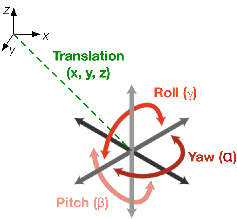
Fig. 1: Localization estimates the six degree of freedom (6 DoF) pose of a body ($x,y,z,\alpha,\beta,\gamma$).

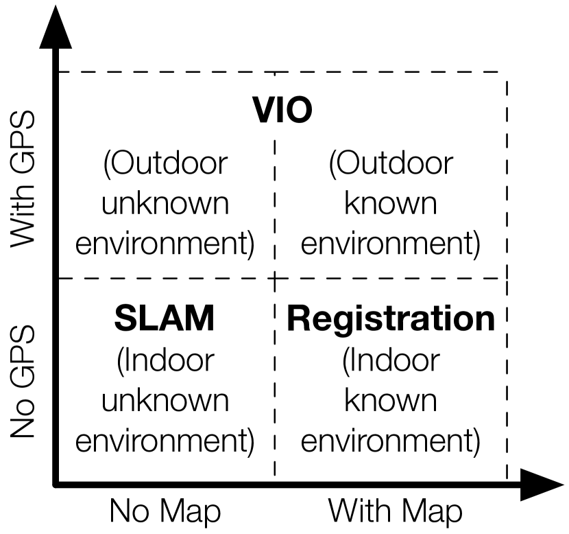
Fig. 2: Taxonomy of real-world environments. Each environment prefers a particular localization algorithm.

These sensors are relatively cheap (below $1,000 combined [6, 4, 1]). We assume that they are available for localization, as in virtually all of today’s autonomous machines.

III One Algorithm Does Not Fit All

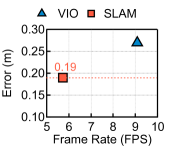
(a) Indoor unknown environment. SLAM provides the best accuracy.

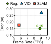
(b) Indoor known environment. Registration has the best accuracy.

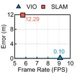
(c) Outdoor unknown environment. VIO is best in accuracy.

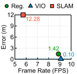
(d) Outdoor known environment. VIO is best in accuracy.

Fig. 3: Localization error vs. performance trade-off in the four operating scenarios, each requiring a particular localization algorithm to maximize accuracy. Note that registration does not apply to scenarios without a map. We use a combination of the KITTI Odometry dataset [38] and our in-house dataset to cover all four scenarios. Results are averaged across all frames.

Hardware design must target an efficient and broadly applicable software base to begin with. By analyzing three fundamental categories of localization algorithms, we find that no one single algorithm applies to all operating scenarios. A flexible localization framework that adapts to different scenarios is needed in practice. While a general-purpose processor easily provides the flexibility, the tight performance requirements call for hardware acceleration.

Operating Environment

Autonomous machines usually have to operate under different scenarios to finish a task. For instance, in one of our commercial deployments, logistics robots transfer cargo between warehouses in an industrial park; during normal operations the robots roughly spend 50% of the time navigating outdoor and 50% of the time inside pre-mapped warehouses. When the robots are moved to a different section of the park (to optimize the overall efficiency), the robots would spend a few days mapping new warehouses.

In principle, real-world environments can be classified along two dimensions for localization purposes as shown in Fig. 2: the availability of a pre-constructed map and the availability of a direct localization sensor, mainly the GPS. First, an environment’s map could be available depending on whether the environment has been previously mapped, i.e., known to the autonomous machine. A map could significantly ease localization because the map provides a reliable frame of reference. Second, depending on whether the environment is indoor or outdoor, GPS could provide absolute positioning information that greatly simplifies localization.

Overall, four scenarios exist in the real-world:

• $<$No GPS, No Map$>$: indoor unknown environment;

• $<$No GPS, With Map$>$: indoor known environment;

• $<$With GPS, No Map$>$: outdoor unknown environment.

• $<$With GPS, With Map$>$: outdoor known environment.

Localization Algorithms

To understand the most fitting algorithm in each scenario, we analyze three fundamental categories of localization algorithms [52, 19] that are: 1) complementary to each other in requirements and capabilities, 2) well-optimized by algorithmic researchers, and 3) widely used in industry. These localization algorithms are:

• Registration: It calculates the 6 DoF pose against a given map. Given the current camera observation $\mathbf{F}$ and the global map $\mathbf{G}$, registration algorithms calculate the 6 DoF pose that transforms $\mathbf{F}$ to $\mathbf{F}^{\prime}$ in a way that minimizes the Euclidean distance (i.e., error) between $\mathbf{F}^{\prime}$ and $\mathbf{G}$. We use the “bag-of-words” framework [36, 66, 3], which is the backbone of many products such as iRobot [7].

• VIO: A classic way of localization without an explicit map is to formulate localization as a probabilistic nonlinear state estimation problem using Kalman Filter (KF), which effectively calculates the relative pose of an autonomous machine with respect to the starting point. Common KF extensions include Extended Kalman Filter (EKF) [51] and Multi-State Constraint Kalman Filter (MSCKF) [64]. Since KF-based methods often appear in a VIO system [55, 54, 55, 88, 79], this paper simply refers to them as VIO.

  In our experiments, we use a MSCKF-based framework [79, 10] due to its superior accuracy compared to other state estimation algorithms. For instance on the EuRoC dataset, MSCKF accuracy on average 0.18m error reduction over EKF [79]. MSCKF is also used by many products such as Google ARCore [15].

  Since VIO calculates the relative trajectory using past observations, its localization errors could accumulate over time [22]. One effective mitigation is to provide VIO with the absolute positioning information through GPS. When stably available, GPS signals help the VIO algorithm relocalize to correct the localization drift [27]. VIO coupled with GPS is often used for outdoor navigation such as in DJI drones [8].

• SLAM: It simultaneously constructs a map while localizing an agent within the map. SLAM avoids the accumulated errors in VIO by constantly remapping the global environment and closing the loop. SLAM is usually formulated as a constrained optimization problem, often through bundle adjustment [43]. SLAM algorithms are used in many robots [11] and AR devices (e.g., Hololens) [5]. We use the widely-used VINS-Fusion framework [73, 14] for experiments.

Note that the design space of VIO and SLAM is broader than the specific algorithms we target. For instance, VIO could use factor-graph optimizations [78] rather than KF. We use VIO to refer to algorithms using probabilistic state estimation without explicitly constructing a map, and uses SLAM to refer to global optimization-based algorithms that construct a map. It is these fundamental classes of algorithms that we focus on.

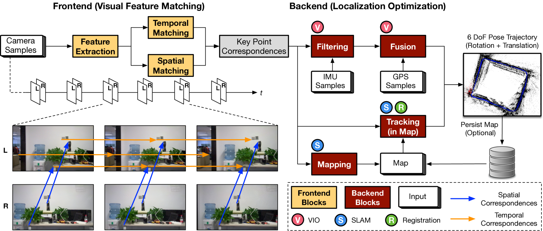
Fig. 4: Overview of our unified localization algorithm framework that adapts to different operating environments. The goal of our framework is to provide an efficient algorithm target for acceleration. The algorithm consists of a vision frontend and an optimization backend. The frontend establishes feature correspondences and is always activated. The backend operates under three modes, each activated in a particular operating scenario. Essentially, our localization framework fuses the three primitive localization algorithms (i.e. registration, VIO, and SLAM) by sharing common building blocks. This strategy preserves the accuracy under each scenario while minimizing algorithm-level redundancies.

Accuracy Characterizations

We find that there is no single localization algorithm that fits all. Instead, each operating environment tends to prefer a different localization algorithm to minimize error. Fig. 3a through Fig. 3d show the root-mean-square error (RMSE) ($y$-axis) and the average performance ($x$-axis) of the three localization algorithms under the four scenarios above, respectively. Since localization algorithm implementations today target CPUs [79, 67], we collect the performance data from a four-core Intel Kaby Lake CPU. See Sec. VII-A for a detailed setup.

In an indoor environment without a map, Fig. 3a shows that SLAM delivers much lower error than VIO (0.19 m vs. 0.27 m). The registration algorithm is not applicable in this case as it requires a map. We do not supply the GPS signal to the VIO algorithm here due to the unstable signal reception; supplying unstable GPS signals would worsen the VIO accuracy. The data shows that VIO lacks the relocalization ability to correct accumulated drifts without GPS.

When an indoor environment has a pre-constructed map, registration achieves higher accuracy while operating at a higher frame rate than SLAM as shown in Fig. 3b. Specifically, the registration algorithm has only a 0.15 meter localization error while operating at 8.9 FPS. VIO almost doubles the error (0.27 m) due to drifts, albeit operating as a slightly higher frame rate (9.1 FPS).

VIO becomes the best algorithm outdoor, both with (Fig. 3d) or without a map (Fig. 3c). VIO achieves the highest accuracy with the help of GPS (0.10 m error) and is the fastest, Pareto-dominating the other two. Even with a pre-constructed map (Fig. 3d), registration still has a much higher error (1.42 m) than VIO; SLAM is the slowest and has a significantly higher error due to difficulties to adapt to changing lightning conditions and drifts. Note that our SLAM error (12.28 m) is lower than prior SLAM work [56] (21 m))

Fig. 2 summarizes the algorithm affinity of each operating scenario to maximize accuracy: indoor environment with a map prefers registration; indoor environment without a map prefers SLAM; outdoor environment prefers VIO. As an autonomous machine often operates under different scenarios, a localization system must simultaneously support the three algorithms so as to be useful in practice.

IV Unified Localization Framework

We propose a localization algorithm framework that adapts to different operation environments, providing a desirable software target for hardware acceleration (Sec. IV-A). By characterizing the performance of the new algorithm framework, we identify lucrative acceleration candidates that, when accelerated, would significantly reduce the overall localization latency and latency variation (Sec. IV-B).

IV-A Algorithm Framework

We propose a localization framework that flexibly adapts to different operating environments. Fig. 4 shows our algorithmic framework. Our strategy is to capture general patterns and to share common building blocks across each of the three primitive algorithms (i.e., registration, VIO, and SLAM). In particular, we find that the three primitive algorithms share the same two-phase design consisting of a visual feature matching phase and a localization optimization phase. While the optimization technique differs in the three primitive algorithms, the feature matching phase is the same.

Decoupled Framework

Our framework consists of a shared vision frontend, which extracts and matches visual features and is always activated, and an optimization backend, which has three modes—registration, VIO, and SLAM—each triggered under a particular operating scenario (Fig. 2). Each mode forms a unique dataflow path by activating a set of blocks in the backend as shown in Fig. 4.

Below we describe each block in the framework. Each block is directly taken from the three individual algorithms (Sec. III), which have been well-optimized and used in many products. While some components have been individually accelerated before [72, 33], it is yet known how to provide a unified architecture to efficiently support these components in one system, which is the goal of our hardware design.

Frontend

The visual frontend extracts visual features to find correspondences in consecutive observations, both temporally and spatially, which the backend uses to estimate the pose. In particular, the frontend consists of three blocks.

• Feature Extraction The frontend first extracts key feature points, which correspond to salient landmarks in the 3D world. Operating on feature points, as opposed to all image pixels, improves the robustness and compute-efficiency of localization. In particular, key points are detected using the widely-used FAST feature [74]; each feature point is associated with an ORB descriptor [75] in preparation for spatial matching later.

• Stereo Matching This block matches key points spatially between a pair of stereo images (from the left and right cameras). We use the widely-used blocking matching method [48] based on the ORB descriptor of each feature point calculated before [21, 75].

• Temporal Matching This block establishes temporal correspondences by matching the key points of two consecutive images. Instead of searching for matches, this block tracks feature points across frames using the classic Lucas-Kanade optical flow method [59].

Backend

The backend calculates the 6 DoF pose from the visual correspondences generated in the frontend. Depending on the operating environment, the backend is dynamically configured to execute in one of the three modes, essentially providing the corresponding primitive algorithm. To that end, the backend consists of the following blocks:

• Filtering This block is activated only in the VIO mode. It uses Kalman Filter to integrate a series of measurements observed over time, including the feature correspondences from the frontend and the IMU samples, to estimate the pose. We use MSCKF [64], a Kalman Filter framework that keeps a sliding window of past observations rather than just the most recent past.

• Fusion This block is activated only in the VIO mode. It fuses the GPS signals with the pose information generated from the filtering block, essentially correcting the cumulative drift introduced in filtering. We use a loosely-coupled approach [88], where the GPS positions are integrated through a simple EKF [51].

• Mapping This block is activated only in the SLAM mode. It uses the feature correspondences from the frontend along with the IMU measurements to calculate the pose and the 3D map. This is done by solving a non-linear optimization problem, which minimizes the projection errors (imposed by the pose estimation) from 2D features to 3D points in the map. The optimization problem is solved using the Levenberg-Marquardt (LM) method [63]. We target an LM implementation in the Ceres Solver, which is used in products such as Google’s Street View [2]. In the end, the generated map could be optionally persisted offline and later used in the registration mode.

• Tracking This block is activated both in the registration and the SLAM mode. Using the bag-of-words place recognition method [36, 66], this block estimates the pose based on the features in the current frame and a given map. In the registration mode, the map is naturally provided as the input. In the SLAM mode, tracking and mapping are executed in parallel, where the tracking block uses the latest map generated from the mapping block, which continuously updates the map.

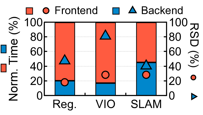
Fig. 5: Latency distribution and relative standard deviation (RSD) of frontend and backend in three modes.

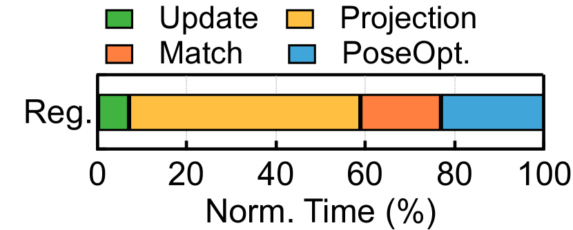
Fig. 6: Latency distribution in registration backend.

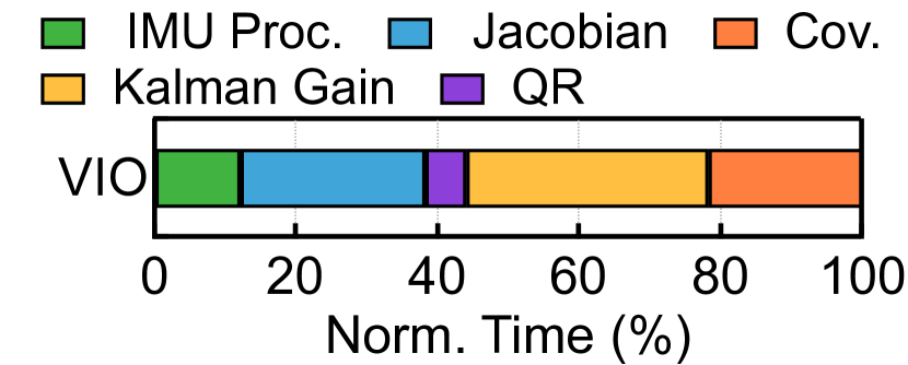
Fig. 7: Latency distribution in VIO backend.

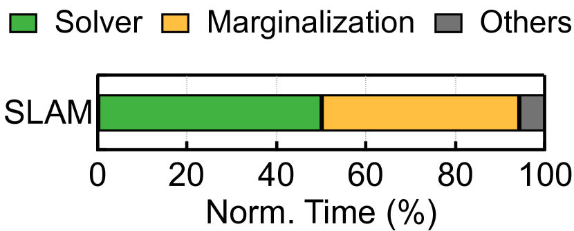
Fig. 8: Latency distribution in SLAM backend.

Accuracy and Performance

Our software framework is accurate. On the popular (indoor) drone dataset EuRoC [20], our algorithm has a relative trajectory error of 0.28% (registration) – 0.42% (SLAM), on par with prior algorithms, whose errors are within the 0.1% to 2% range [34]. On the (outdoor) KITTI dataset [38], our algorithm has a negligible error ($<$ 0.01% error) using VIO+GPS.

Our software framework is about 4% faster than the dedicated algorithms, because we remove their dependencies on the Robot Operation System (ROS), which is a common framework (libraries, runtime services) on top of Linux for developing robotics applications but is known to incur non-trivial overheads [70, 81]. Our framework is thus a clean target for performance characterizations and acceleration.

IV-B Latency Characterizations

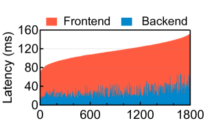
(a) Per-frame latency breakdown between frontend and backend.

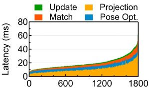
(b) Latency breakdown in backend.

Fig. 9: Latency variation in the registration mode.

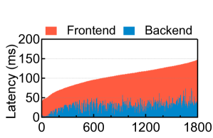
(a) Per-frame latency breakdown between frontend and backend.

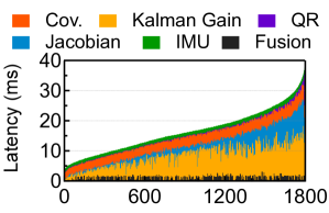
(b) Latency breakdown in backend.

Fig. 10: Latency variation in the VIO mode.

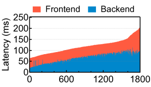
(a) Per-frame latency breakdown between frontend and backend.

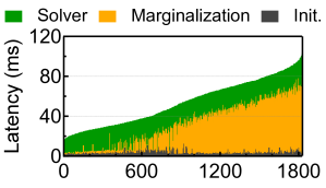
(b) Latency breakdown in backend.

Fig. 11: Latency variation in the SLAM mode.

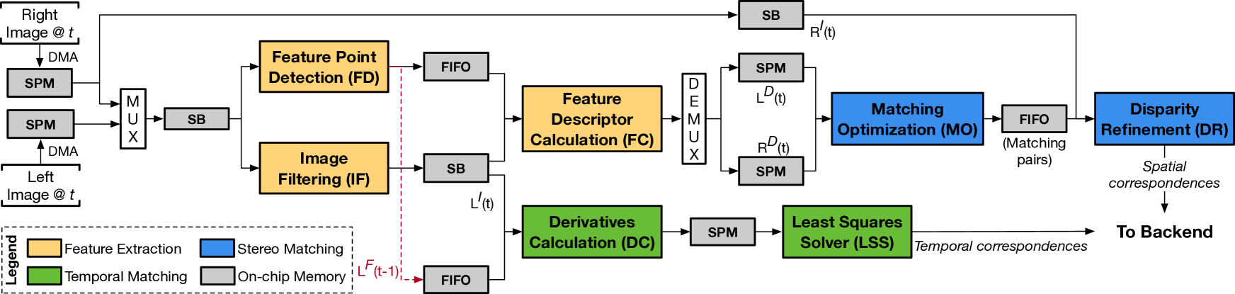
Fig. 12: Frontend architecture, which consists of three blocks: feature extraction, optical flow, and stereo matching. The left and right camera streams are time-multiplexed in the feature extraction block to save hardware resources. On-chip memories are customized in different ways to suit different types of data reuse: stencil buffer (SB) supports stencil operations, FIFO captures sequential accesses, and scratchpad memory (SPM) supports irregular accesses.

Latency Distribution

We find that the frontend contributes significantly to the end-to-end latency across all three scenarios. Since the frontend is shared across different backend modes, accelerating the frontend would lead to “universal” performance improvement. Fig. 8 shows the average latency distribution between the frontend and the backend across the three scenarios. The frontend time varies from 55% in the SLAM mode to 83% in the VIO mode. The SLAM backend is the heaviest because it iteratively solves a complex non-linear optimization problem.

While the frontend is a lucrative acceleration target, backend time is non-trivial too, especially after the frontend is accelerated. Fig. 8, Fig. 8, and Fig. 8 show the distribution of different blocks within each backend mode. Marginalization in SLAM, computing Kalman gain in VIO, and projection in registration are the biggest contributors to the three backend modes. Interestingly, these three kernels also contribute significantly to the backend variation, which we analyze next.

Latency Variation

Localization has high latency variation under all three modes.  Fig. 9a, Fig. 9a, and Fig. 10a show the per-frame latency distribution between the frontend and the backend in the registration, VIO, and SLAM mode, respectively. The data is sorted by the total latency. The longest latency in the SLAM mode is over 4$\times$ longer than the shortest latency. The difference is over 2$\times$ in the registration mode.

Compared to the frontend, the backend exhibits higher variation. We use relative standard deviation (RSD, a.k.a., coefficient of variation), which is defined as the ratio of the standard deviation to the mean of a distribution [35], to compare the frontend and backend variation. The right $y$-axis in Fig. 8 compares the RSDs of the frontend and backend in the three modes. The difference is most significant in the VIO mode where the RSDs of the frontend and the backend are 47.3% and 81.1%, respectively.

We further breakdown the latency variation in each backend mode, shown in Fig. 9b, Fig. 9b, and Fig. 10b. In each backend there is a single biggest contributor to the variation: camera model projection in registration, computing Kalman gain in VIO, and marginalization in SLAM. They match the overall latency contributors described before.

V Frontend Architecture

This section describes our frontend accelerator. After an overview (Sec. V-A), we discuss two optimizations that 1) improve the performance by exploiting unique task-level parallelisms (Sec. V-B) and 2) reduce on-chip memory usage by capturing data locality at the FPGA synthesis time (Sec. V-C).

V-A Overview and Design Principles

Fig. 12 provides an overview of the architecture. The input (left and right) images are streamed through the DMA and double-buffered on-chip. The on-chip memory design mostly allows the frontend to access DRAM only at the beginning and the end of the pipeline as we will discuss later.

The two images go through three blocks: feature extraction, spatial matching, and temporal matching. Each block consists of multiple tasks. For instance, the feature extraction block consists of three tasks: feature point detection, image filtering, and descriptor calculation.

The feature extraction block is exercised by both the left and right images. The feature points in the left image at time $t-1$ ($L^{F}_{t-1}$) are buffered on-chip, which are combined with the left image at time $t$ ($L^{I}_{t}$) to calculate the temporal correspondence at $t$. Meanwhile, the feature descriptors in both images at $t$ ($L^{D}_{t}$ and $R^{D}_{t}$) are consumed by the stereo matching block to calculate the spatial correspondences at $t$. The temporal and spatial correspondences are about 2 – 3 KB on average; they are transmitted to the backend.

V-B Exploiting Task-Level Parallelisms

Understanding the Parallelisms

At the high-level, feature extraction (FE) consumes both the left and right images, which are independent and could be executed in parallel. Stereo matching (SM) must wait until both images finish the Feature Descriptor Calculation (FC) task in the FE block, because SM requires the feature points/descriptors generated from both images. Temporal matching (TM) operates only on the left image and is independent of SM. Thus, TM could start whenever the left image finishes the image filtering (IF) task in FE. The IF task and the feature point detection (FD) task operate in parallel in FE.

TM consists of two serialized tasks: derivatives calculation (DC), whose outputs drive a (linear) least squares solver (LSS). SM consists of a matching optimization (MO) task, which provides initial spatial correspondence by comparing hamming distances between feature descriptors, and a disparity refinement (DR) task which refines the initial correspondences through block matching.

Design

TM latency is usually over 10$\times$ lower than SM latency. Thus, the critical path is FD $\rightarrow$ FC $\rightarrow$ MO $\rightarrow$ DR. The critical path latency is in turn dictated by the SM latency (MO+DR), which is roughly 2 – 3$\times$ higher than the FE latency (FD+FC). Therefore, we pipeline the critical path between the FE and the SM. Pipelining improves the frontend throughput, which is dictated by the latency of SM.

Interestingly, the FE hardware resource consumption roughly doubles the resource consumption of TM and SM combined, as FE processes raw input images whereas SM and TM process only key points ($<$0.1% of total pixels). Thus, we time-share the FE hardware between the left and right images. This reduces hardware resource consumption, but does not hurt the throughput since FE is much faster than SM.

V-C Capturing Data Locality By Synthesis-Time Specialization

We carefully design on-chip memory structures to capture three fundamental types of intra-task and inter-task data reuses patterns in the frontend (Fig. 12). First, the frontend algorithm has many stencil operations, such as convolution in IF and block-matching in MO. We propose a stencil buffer (SB) design to capture data reuse in stencil operations. Second, many stencil operations read from a list sequentially, for which a FIFO is suitable. For instance, FC operates on feature points detected before one after another. Finally, some stages (e.g., MO) exercise arbitrary memory accesses, for which a generic scratchpad memory (SPM) is more suitable. We use generic FIFO and SPM structures, and describe our unique SB below.

Basic Stencil Buffer Design

General data reuse in stencil operations, e.g., convolution, has been extensively explored [24, 23, 50]. However, since we target FPGA, our SBs are designed to specialize for specific stencil sizes in a given algorithm when we synthesize an FPGA design.

Fig. 14 overviews the SB microarchitecture using an example where two stencil operations share the same input. This is similar to our pipeline where FD and IF share the same input image. In this example, the first stencil operation has a size of $4\times 3$ and the second stencil operation has a size of $3\times 3$. Thus, the SB buffers 4 lines from the input image. We use 4 cascaded FIFOs, followed by two shift registers, each of which contains the pixels in one stencil window. Each cycle, each FIFO pops one pixel, which is written into both the corresponding shift register(s) and the previous FIFO. The first three FIFOs write to both shift registers, whereas the last FIFO writes to only the first shift register.

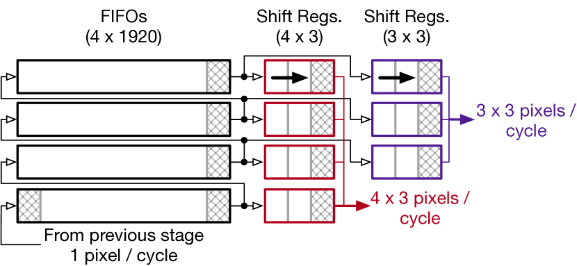
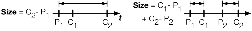
Fig. 13: Stencil buffer (SB) design. An SB consists of a set of (4 here) sequentially cascaded FIFOs that are connected to one or more (2 here) shift registers. Each cycle, one pixel enters the SB and 4 pixels enter the shift registers.

Fig. 14: SB optimizations. $P_{1}$ and $P_{2}$ denote production cycles; $C_{1}$, and $C_{2}$ denote consumption cycles. When $P_{2}>C_{1}$, replicating pixels in two SBs requires less memory than sharing one SB at the expense of one extra memory read.

Reducing SB Sizes by Redundant DRAM Accesses

Our SB design is reminiscent of the traditional line buffers [25, 83, 44, 45] with a critical difference. The objective of traditional line buffers is to minimize DRAM traffic such that every input element is read from DRAM once. For the localization frontend, doing that would bloat the buffer size, because the consumption and production of a pixel could be millions of cycles apart in a long stencil pipeline. Our design reads pixels multiple times from the DRAM to significantly save on-chip buffer storage. Let us explain below.

Generally, if a pixel is pushed into the SB at cycle $P_{1}$ and consumed by two stencil operations at cycle $C_{1}$ and $C_{2}$, the SB size must be at least $max(C_{1},C_{2})-P_{1}$, because a new pixel is pushed into the SB every cycle. Between two consumption cycles, the pixel occupies the SB space without being used. If $|C_{1}-C_{2}|$ is large, space waste is significant. This scenario is manifested in our algorithm, where DR reads from the same image that IF and FD read from, but DR is millions of cycles later than IF and FD in the pipeline.

Instead, we use two SBs and read each pixel twice, essentially replicating the pixels in the two SBs. The total SB size would be $(C_{1}-P_{1})+(C_{2}-P_{2})$, where $P_{1}$ and $P_{2}$ denote the two cycles when the pixel is read. When $P_{2}>C_{1}$, reading pixels multiple times reduces the total SB size. Given the stencil sizes in a particular algorithmic configuration, which is statically known, we first decide whether replicating pixels is beneficial and then calculate the size of each SB, which we specify when synthesizing the FPGA design.

VI Backend System

The backend has high latency variation, especially after the frontend is accelerated, and thus is an ideal acceleration target. We first show that the backend kernels share common building blocks, which we exploit to design a flexible and efficient architecture substrate (Sec. VI-A). Due to the large variation, accelerating the backend is not always beneficial; we exploit the execution behaviors of the backend kernels to design a lightweight runtime scheduler, which ensures that backend acceleration reduces variation without increasing overall latency (Sec. VI-B).

VI-A Backend Architecture

Building Blocks

Recall from Sec. IV-B that the each backend mode inherently possesses a kernel that contributes significantly to both the overall latency and the latency variation: camera model projection under the registration mode, computing Kalman gain under the VIO mode, and marginalization under the SLAM mode. Accelerating these kernels reduces the overall latency and latency variation.

While it is possible to spatially instantiate separate hardware logic for each kernel, it would lead to resource waste. This is because the three kernels share common building blocks. Fundamentally, each kernel performs matrix operations that manipulate various forms of visual features and IMU states. Tbl. I decomposes each kernel into different matrix primitives.

TABLE I: Latency variation-contributing kernels in the backend are composed of common matrix operations.

Building Block	Projection	Kalman Gain	Marginalization
Matrix Multiplication	✓	✓	✓
Matrix Decomposition		✓	✓
Matrix Inverse			✓
Matrix Transpose		✓	✓
Fwd./Bwd. Substitution		✓	✓

For instance, the projection kernel in the registration mode simply multiplies a $3\times 4$ camera matrix $\mathbf{C}$ with a $4\times M$ matrix $\mathbf{X}$, where $M$ denotes the number of feature points in the map (each represented by 4D homogeneous coordinates). The Kalman gain $\mathbf{K}$ in VIO is computed by:

$$\mathbf{S} =\mathbf{H}\times\mathbf{P}\times\mathbf{H}^{T}+\mathbf{R}$$ (1a)

$$\mathbf{S}\times\mathbf{K} =\mathbf{P}\times\mathbf{H}^{T}$$ (1b)

where $\mathbf{H}$ is the Jacobian matrix of the function that maps the true state space into the observed space, $\mathbf{P}$ is the covariance matrix, and $\mathbf{R}$ is an identity noise matrix. Calculating $\mathbf{K}$ requires solving a system of linear equations, which is implemented by matrix ($\mathbf{S}$) decomposition followed by forward/back-substitution. Marginalization combines all five operations; its formulation is omitted here for simplicity.

Design

The backend specializes the hardware for the five matrix operations in Tbl. I, which the three backend kernels are then mapped to. These matrix operations are low-level enough to allow sharing across different backend kernels but high-level enough to reduce the control flows, which are particularly inefficient to implement on FPGAs.

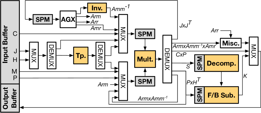
Fig. 15: Backend architecture. It consists of five basic building blocks for matrix operations: inverse (Inv.), decomposition (Decomp.), transpose (Tp.), multiplication (Mult.), and forward/backward-substitution. “AGX” is the address generation logic, and “Misc.” contains the rest of the logic not included in any above (e.g., addition).

Fig. 15 shows the backend architecture. The input and output are buffered on-chip and DMA-ed from/to the host. The inputs to each matrix block are stored in the SPMs. The input matrices must be ready before an operation starts. Importantly, the SPMs can not be replaced by SBs (Fig. 14) as in the frontend, because these matrix operations, unlike convolution and block matching in the frontend, are not stencil operations.

The architecture accommodates different matrix sizes by exploiting the inherent blocking nature of matrix operations (e.g., multiplication, decomposition), where the output could be computed by iteratively operating on different blocks of the input matrices. Thus, the compute units have to support computations for only a block, although the SPMs need to accommodate the size of the entire input matrices.

Optimization

We exploit unique characteristics inherent in various matrices to further optimize the computation and memory usage. The $\mathbf{S}$ matrix is inherently symmetric (Equ. 1a). Thus, the computation and storage cost of $\mathbf{S}$ can naturally be reduced by half. In addition, the matrix that requires inversion in marginalization, $A_{mm}$, is a symmetric matrix with a unique blocking structure of $\begin{bmatrix}A&B\\ C&D\end{bmatrix}$, where $A$ is a diagonal matrix and $D$ is a $6\times 6$ matrix, where 6 represents the number of degrees of freedom in a pose to be calculated. Therefore, the inversion hardware is specialized for a $6\times 6$ matrix inversion combined with simple reciprocal structures.

VI-B Runtime Scheduling

Offloading backend kernels to the backend accelerator is not always beneficial due to the overhead of data transfer, especially when the size of the matrix involved in a kernel is small. For instance, in many frames the marginalization time is below 1 ms (Fig. 10b), in which case offloading marginalization degrades performance.

The latency of each kernel highly correlates with the sizes of the matrices that it operates on, which in turn depends on information calculated in the frontend. Using the same 1,800 frames profiled in Sec. IV-B, Fig. 16a shows that the projection latency of a frame ($y$-axis) increases almost linearly with the number of points in the current map ($x$-axis). Fig. 16b shows that the latency of computing the Kalman gain in a frame ($y$-axis) scales with $\mathbf{H}$’s height ($x$-axis), which is dictated by the number of key points in a frame extracted by the frontend. Fig. 16c shows that the marginalization latency increases with the number of feature points, too.

(a) Projection.

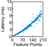
(b) Kalman gain.

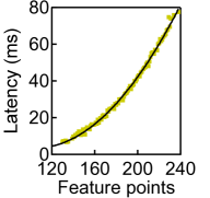
(c) Marginalization.

Fig. 16: The backend kernels’ latency is dictated by the size of matrices that they operate on.

Leveraging this insight, we design a lightweight software scheduler, which offloads the backend only when the latency could be reduced. The scheduler first estimates the CPU execution time using simple regression models constructed offline, as illustrated in Fig. 16. In particular, the projection time is fit using a linear model whereas the other two kernerls’ times are estimated by quadratic models. The scheduler then estimates the acceleration time from the latency profiles of the five building blocks and the data transfer bandwidth, both obtained offline. The scheduler triggers the accelerator when the CPU time would be longer than acceleration time.

VII Evaluation

VII-A Experimental Setup

Hardware Platform

We build an FPGA prototype (Edx-Car) and evaluate it on our commercial autonomous vehicle. We use a Xilinx Virtex-7 XC7V690T FPGA board [13] connected to a PC machine, which has a four-core Intel Kaby Lake CPU (1.6 GHz and 9 MB LLC) and 8 GB memory. To show the flexibility and general applicability of our design framework, we also build another prototype targeting drones (Edx-Drone), for which we use a Zynq Ultrascale+ ZU9CG board [16], which integrates a quad-core ARM Cortex-A53 CPU with an FPGA on the same chip.

The actual accelerator implementations on both instances are almost the same except that Edx-Car uses a larger matrix multiplication/decomposition unit and larger line-buffers and SPMs to deal with a higher input resolution.

The FPGA is directly interfaced with the cameras and IMU/GPS sensors. The host and the FPGA accelerator communicate three times in each frame: the first time from the FPGA, which transfers the frontend results and the IMU/GPS samples to the host; the second time from the host, which passes the inputs of a backend kernel (e.g., the $\mathbf{H}$, $\mathbf{P}$, and $\mathbf{R}$ matrices to calculate Kalman gains) to the FPGA, and the last time transferring the backend results back to the host.

For Edx-Car, FPGA reads data from PC through PCI-e 3.0, with a max bandwidth of 7.9 GB/s. For Edx-Drone, the FPGA reads data from DRAM through the AXI4 bus, with a max bandwidth of 1.2 GB/s.

Baselines

To our best knowledge, today’s localization systems are mostly implemented on general-purpose CPU platforms. Thus, we compare Edx-Car against the software implementation on the PC machine without the FPGA, and compare Edx-Drone against the software implementation on the quad-core Arm Cortex-A57 processor on the TX1 platform [12], a representative mobile platform today. To obtain stronger baselines, the software implementations leverage multi-core and the SIMD capabilities of the CPUs. For a comprehensive evaluation, we will also compare against GPU and DSP implementations in Sec. VII-H.

Dataset

For Edx-Drone, we use EuRoC [20] (Machine Hall sequences), a widely-used drone dataset. Since EuRoC contains only indoor scenes, we complement EuRoC with our in-house outdoor dataset. The two datasets combined have 50% outdoor frames, 25% indoor frames without map, and 25% indoor frames with map. The input images are sized to the $640\times 480$ resolution. For Edx-Car, we use KITTI Odometry [38] (grayscale sequence), which is a widely-used self-driving car dataset. Similarly, since KITTI contains only outdoor scenes, we complement it with our in-house dataset for indoor scenes. The distribution of the three scenes is the same as above. The input images are uniformly sized to the $1280\times 720$ resolution. The energy results are averaged across all the evaluated frames.

To evaluate the effect of the runtime scheduler (Sec. VI-B), we use 25% of the frames in the datasets to construct the regression models offline, and evaluate on the rest 75%.

VII-B Resource Consumption

TABLE II: FPGA resource consumption of Edx-Car and Edx-Drone and their utilizations on the actual FPGA boards. Data is obtained after the design passes post-place & route timing. The “N.S.” columns denote the hypothetical resource usage if we do not share the frontend and the building blocks in the backend across the three modes.

Resource	Car	Virtex-7	N.S.	Drone	Zynq	N.S.
LUT	350671	80.9%	795604	231547	84.5%	659485
Flip-Flop	239347	27.6%	628346	171314	31.2%	459485
DSP	1284	35.6%	3628	1072	42.5%	3064
BRAM	5.0	87.5%	13.2	3.67	92.3%	10.6

We show the FPGA resource usage in Tbl. II. Overall, Edx-Car consumes more resources than Edx-Drone as the former uses larger hardware structures to cope with higher input resolutions (Sec. VII-A). To demonstrate the effectiveness of our hardware design that shares the frontend and the various backend building blocks across the three modes (Tbl. I), the “N.S.” columns show the hypothetical resource consumption without sharing these structures in both instances. Resource consumption of all types would more than double, exceeding the available resources on the FPGA boards.

Frontend dominates the resource consumption. In Edx-Car, the frontend uses 83.2% LUT, 62.2% Flip-Flop, 80.2% DSP, and 73.5% BRAM of the total used resource; the percentages in Edx-Drone are similar. In particular, feature extraction consumes over two-thirds of frontend resource, corroborating our design decision to multiplex the feature extraction hardware between left and right camera streams (Sec. V-B).

Other Storage Requirements

The MSCKF window size is 30, which translates to a total storage requirement is 1.2 MB (state vector, covariance matrix, Jacobian matrix, Kalman gain). These data structures initially reside in DRAM and are transferred to the FPGA depending on what matrix operations are offloaded. The dictionary for loop detection is about 60 MB, which initially resides in the DRAM. Only the Projection kernel of loop closure is offloaded to FPGA (Tbl. I).

VII-C Overall Results

Car Results

We compare the average frame latency and variation between the baseline and Edx-Car in Fig. 17a. We show the overall results as well as the results in the three modes separately. The end-to-end frame latency is reduced by 2.5$\times$, 2.1$\times$, and 2.0$\times$ in registration, VIO, and SLAM mode, respectively, which leads to overall 2.1$\times$ speedup. Edx-Car also significantly reduces the variation. The standard deviation (SD) is reduced by 58.4%. The latency reduction directly translates to higher throughput, which reaches 17.2 FPS from 8.6 FPS, as shown in Fig. 19. Further pipelining the frontend with the backend improves the FPS to 31.9.

The energy is also significantly reduced. Fig. 19 compares the energy per frame between the baseline and Edx-Car. With hardware acceleration, Edx-Car reduces the average energy by 73.7%, from 1.9 J to 0.5 J per frame.

Drone Results

We show the results of Edx-Drone in Fig. 17b. The frame latency has a speedup of 2.0$\times$, 1.9$\times$, and 1.8$\times$ in the three modes, respectively, which leads to a 1.9$\times$ overall speedup. The overall SD is reduced by 42.7%. The average throughput is improved from 7.0 FPS to 22.4 FPS. The average energy per frame is reduced by 47.4% from 0.8 J to 0.4 J per frame. The energy saving is lower than Edx-Car because the FPGA static power stands out as Edx-Drone reduces the dynamic power.

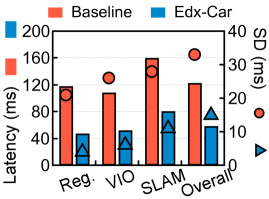
(a) Latency and variation improvement on Edx-Car.

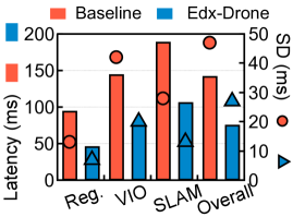
(b) Latency and variation improvement on Edx-Drone.

Fig. 17: Overall system latency and variation reduction.

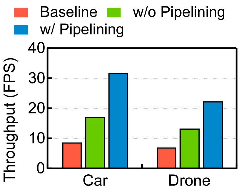
Fig. 18: FPS of baseline and Eudoxus with and without frontend/backend pipelining.

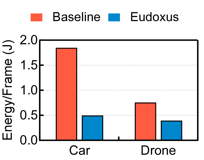
Fig. 19: Energy per frame comparison between baseline and Eudoxus.

VII-D Frontend Results

Car Results

We show the frontend latency results of Edx-Car in Fig. 20a. We break down the frontend latency of Edx-Car into two components: feature extraction (FE) and stereo matching (SM). Note that the temporal matching is hidden behind the critical path, and thus does not contribute to the latency. Compared to the baseline, the average frontend latency is reduced from 92.4 $ms$ to 42.7 $ms$, a 2.2$\times$ speedup. The SM dominates the frontend latency, further confirming our design decision to multiplex the FE hardware between left and right camera streams (Sec. V-B).

Fig. 20b compares the throughput of the baseline with two versions of Edx-Car, one that pipelines FE and SM and the other that does not. With pipelining, the frontend throughput is 44.0 FPS, higher than the overall system throughput of 31.9 (Fig. 19). Note that the throughput without pipelining is 26.1, lower than the overall throughput. This indicates that without FE/SM pipelining the frontend is the system bottleneck, while pipelining pushes the bottleneck to the backend.

Drone Results

The frontend latency and throughput improvements in Edx-Drone are shown in Fig. 20a and Fig. 20b, respectively, too. Edx-Drone achieves 2.2$\times$ latency speed up and 4.0$\times$ throughput speedup with pipelining. The frontend latency of Edx-Drone is slightly faster than that of Edx-Car. This is because drones deal with a 3$\times$ lower image resolution than self-driving cars, leading to lower compute workload overall.

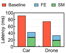
(a) Latency comparison.

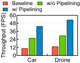
(b) Throughput comparison.

Fig. 20: Frontend acceleration results.

On-chip Memory Design

Owing to our SB optimization (Fig. 14), the SB size is very small while the SPM by far dominates the memory resources. For instance on Edx-Car, SPM consumes about 3.6 MB memory while SB consumes 0.4 MB. Without the SB optimization, the SB size would increase by about 9 MB, far exceeding the FPGA resource provision. This is because a pixel would have to stay in the SB for over 3 million cycles after being consumed by FD/IF and before being consumed by DR (Sec. V-C).

VII-E Backend Results

Car Results

We show the backend performance results of Edx-Car in Fig. 21a. The left $y$-axis shows the latency, and the right $y$-axis shows the standard deviation. The average backend latency in the registration model is reduced by 49.4%. The large latency reduction is a direct result of accelerating the Projection kernel, whose latency is reduced by 95.3%. Meanwhile, the backend variation is also significantly reduced. The SD is reduced by 58.7% from 9.6 $ms$ to 4.0 $ms$.

In the VIO mode, the Kalman gain kernel is accelerated by 2.0$\times$, which translates to 16.3% overall backend latency reduction as Kalman gain contributes to about 33.3% of the VIO latency (Fig. 8). The improvements in the SLAM mode are significant. The Marginalization kernel is accelerated by 2.4$\times$, which translates to 30.2% overall backend latency reduction. The SD also reduces from 21.4 $ms$ to 10.9 $ms$.

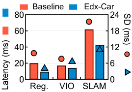
(a) Backend latency and variation improvements of Edx-Car.

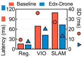
(b) Backend latency and variation improvements of Edx-Drone.

Fig. 21: Backend latency and variation reduction.

Drone Results

Fig. 21b compares the backend latency and latency variation between Edx-Drone and baseline. The backend latency reduction is 16.7%, 38.9%, and 32.7% in the registration, VIO, and SLAM modes, respectively. The SD reductions are 19.4%, 44.4%, and 51.9%, respectively. The per-frame latency comparison figures are omitted due to space limitations. Unlike frontend, the backend is faster on Edx-Car than on Edx-Drone even though the former has to deal with a larger input resolution. This is because the backend accelerator in Edx-Car uses a larger matrix multiplication and decomposition unit.

VII-F Effectiveness of Backend Scheduling

We find that the regression model has a $R^{2}$ value (i.e., coefficient of determination [35]) of 0.83, 0.82, and 0.98 for registration, VIO, and SLAM, respectively, indicating high accuracy. To quantify the effectiveness of the runtime scheduler, we compare it against an oracle scheduler which always correctly schedules the frames. In all three cases, our runtime scheduler results in almost the same speedup compared to the oracle scheduler (less than 0.001% difference).

Using Edx-Car as a case-study, almost all the frames are offloaded to FPGA in the registration and VIO mode. However, only 76.4% frames are offloaded in SLAM. Always offloading SLAM frames increases latency by 8.3%.

VII-G Existing Accelerator Comparison

Existing ASIC/FPGA localization accelerators target different algorithmic variants than ours, so a fair comparison is difficult. Below is our best-effort comparison.

Suleiman et. al. [78] (ASIC VIO) uses factor-graph optimizations. In comparison, our system has slightly higher error (0.28%–0.42% vs. 0.28%) on EuRoC. The ASIC runs at 28–171 FPS whereas Edx-Drone runs at 22.4 FPS on average.

Compared to Li et. al. [56] (ASIC SLAM), our algorithm has a much lower error (0.01% vs. 2.1%) on KITTI. The ASIC runs at 30 – 80 FPS while Edx-Car runs at 31.9 FPS.

Compared to Suleiman et. al. [77] (FPGA VIO), our algorithm has similar error (0.23 $m$ vs. 0.19 $m$) on EuRoC. They run at 5 – 20 FPS while Edx-Drone runs at 22.4 FPS.

We note that: 1) 30 FPS is considered real-time; our FPS could be higher with more capable FPGA platforms, and 2) Eudoxus unifies different algorithms in one design while prior accelerators focus on one algorithm each.

VII-H CPU/GPU/DSP Comparison

Tbl. III presents a comprehensive performance comparison with various CPU/GPU/DSP baselines. Due to space limit, we show the data of only Edx-Car as a case study.

TABLE III: Edx-Car speedup over CPU/GPU/DSP.

Baseline	Speedup ($\times$)
Single-core w/ ROS	3.5
Single-core w/o ROS	3.3
Multi-core w/ ROS	2.2
Multi-core w/o ROS (Our baseline)	2.1
Adreno 530 mobile GPU + CPU	4.4
Hexagon 680 DSP + CPU	2.5
Maxwell mobile GPU + CPU	2.5

Edx-Car has the lowest speedup over the baseline used in this paper (i.e., multi-core without ROS dependencies), indicating that our baseline is optimized. The GPU implementations are slower than CPU, mainly because of the launch/setup time (40 $ms$ on Adreno GPU; batching is unavailable) and the inefficiency in dealing with sparse matrices in SLAM/VIO backend. For this reason, we are not aware of widely-used GPU implementations of end-to-end SLAM/VIO system.

VIII Conclusion and Future Work

Eudoxus identifies and addresses a key challenge in deploying autonomous machines in the real world: efficient and flexible localization under resource constraints. We summarize key lessons we learned and outline a few future directions.

Establishing Proper Software Target for Acceleration

Using data collected from our commercial deployment and standard benchmarks, we show that no existing localization algorithm (e.g., constrained optimization-based SLAM [67, 29, 71], probabilistic estimation-based VIO [61, 64, 49, 60], and registration against the map [67, 65]) is sufficiently flexible to adapt to different real-world operating scenarios. Therefore, accelerating any single algorithm will unlikely be useful in real products. We propose a general-purpose localization algorithm that integrates key primitives in existing algorithms. The new algorithm retains high accuracy of individual algorithms, simplifies our software stack, and provides a desirable acceleration target.

Our initial exploration suggests that the same “one algorithm does not fit all” observation applies to other autonomous machine tasks such as planning and control, suggesting opportunities for software-hardware co-design in the future.

Unified Architecture

The unified algorithm framework enables a unified architecture substrate, a key difference compared to prior localization accelerators on ASIC [78, 56, 86] and FPGA [89, 88, 58, 30, 37, 17, 80] that target only specific algorithms and scenarios. We show that simply stacking dedicated accelerators built for each algorithm (the N.S. columns in Tbl. II) leads to over 2$\times$ resource waste. Additionally, with the same design principle, Eudoxus can be instantiated differently to target different autonomous machines with varying performance requirements and constraints, e.g., drones vs. self-driving cars, as we demonstrate in Sec. VII. The unified methodology and architecture greatly simplify our design and deployment flow, and are instrumental to allow us to expand our product lines going forward.

System-level Optimizations

While many have studied accelerators for individual tasks in localization, such as convolution [72], stereo matching [33, 57], and optical flow [40, 84], an end-to-end localization system necessarily integrates different tasks, and requires us to explore optimizations at the system level [47]. Our hardware design exploits the parallelism and data communication patterns across different tasks, and judiciously applies pipelining, resource-sharing, on-chip buffer specialization to achieve meaningful system-level gains.

Architectural Support for Autonomous Machines

Architectural and systems support for autonomous machines has received increasing attention lately in academia, ranging from accelerating motion planning and control [76, 69, 68], point cloud analytics [31, 32, 85], enabling distributed cognition [42, 62, 41], to benchmarking [82, 18, 39]. We present a case study on localization, which we hope could promote open software stacks and hardware platforms for autonomous machines in the near future, much like today’s machine learning domain.

References

- [1] “Camera price.” [Online]. Available: https://www.amazon.com/s?k=car+camera&ref=nb_sb_noss_1
- [2] “Ceres users.” [Online]. Available: http://ceres-solver.org/users.html
- [3] “Dbow2.” [Online]. Available: https://github.com/dorian3d/DBoW2
- [4] “Gps price.” [Online]. Available: https://www.amazon.com/s?k=GPS&ref=nb_sb_noss_2
- [5] “Highly efficient machine learning for hololens.” [Online]. Available: https://www.microsoft.com/en-us/research/uploads/prod/2018/03/Andrew-Fitzgibbon-Fitting-Models-to-Data-Accuracy-Speed-Robustness.pdf
- [6] “Imu price.” [Online]. Available: https://www.amazon.com/s?k=IMU&ref=nb_sb_noss_2
- [7] “irobot brings visual mapping and navigation to the roomba 980.” [Online]. Available: https://spectrum.ieee.org/automaton/robotics/home-robots/irobot-brings-visual-mapping-and-navigation-to-the-roomba-980
- [8] “Mark: the world’s first 4k drone positioned by visual inertial odometry.” [Online]. Available: https://www.provideocoalition.com/mark-the-worlds-first-4k-drone-positioned-by-visual-inertial-odometry/
- [9] “MIPI Camera Serial Interface 2 (MIPI CSI-2).” [Online]. Available: https://www.mipi.org/specifications/csi-2
- [10] “Msckf vio.” [Online]. Available: https://github.com/KumarRobotics/msckf_vio
- [11] “Slamcore.” [Online]. Available: https://www.slamcore.com/
- [12] “Tx1 datasheet.” [Online]. Available: http://images.nvidia.com/content/tegra/embedded-systems/pdf/JTX1-Module-Product-sheet.pdf
- [13] “Vertex-7 datasheet.” [Online]. Available: https://www.xilinx.com/support/documentation/data_sheets/ds180_7Series_Overview.pdf
- [14] “Vins-fusion.” [Online]. Available: https://github.com/HKUST-Aerial-Robotics/VINS-Fusion
- [15] “Visual inertial fusion.” [Online]. Available: http://rpg.ifi.uzh.ch/docs/teaching/2018/13_visual_inertial_fusion_advanced.pdf#page=33
- [16] “Znyq datasheet.” [Online]. Available: https://www.xilinx.com/support/documentation/data_sheets/ds891-zynq-ultrascale-plus-overview.pdf
- [17] K. Boikos and C.-S. Bouganis, “Semi-dense slam on an fpga soc,” in 2016 26th International Conference on Field Programmable Logic and Applications (FPL). IEEE, 2016, pp. 1–4.
- [18] B. Boroujerdian, H. Genc, S. Krishnan, W. Cui, A. Faust, and V. Reddi, “Mavbench: Micro aerial vehicle benchmarking,” in 2018 51st Annual IEEE/ACM International Symposium on Microarchitecture (MICRO). IEEE, 2018, pp. 894–907.
- [19] A. Budiyono, L. Chen, S. Wang, K. McDonald-Maier, and H. Hu, “Towards autonomous localization and mapping of auvs: a survey,” International Journal of Intelligent Unmanned Systems, 2013.
- [20] M. Burri, J. Nikolic, P. Gohl, T. Schneider, J. Rehder, S. Omari, M. W. Achtelik, and R. Siegwart, “The euroc micro aerial vehicle datasets,” The International Journal of Robotics Research, vol. 35, no. 10, pp. 1157–1163, 2016.
- [21] M. Calonder, V. Lepetit, C. Strecha, and P. Fua, “Brief: Binary robust independent elementary features,” in European conference on computer vision. Springer, 2010, pp. 778–792.
- [22] C. Chen, X. Lu, A. Markham, and N. Trigoni, “Ionet: Learning to cure the curse of drift in inertial odometry,” in Thirty-Second AAAI Conference on Artificial Intelligence, 2018.
- [23] Y.-H. Chen, J. Emer, and V. Sze, “Eyeriss: A spatial architecture for energy-efficient dataflow for convolutional neural networks,” in ACM SIGARCH Computer Architecture News, vol. 44, no. 3. IEEE Press, 2016, pp. 367–379.
- [24] Y. Chen, T. Luo, S. Liu, S. Zhang, L. He, J. Wang, L. Li, T. Chen, Z. Xu, N. Sun et al., “Dadiannao: A machine-learning supercomputer,” in Proceedings of the 47th Annual IEEE/ACM International Symposium on Microarchitecture. IEEE Computer Society, 2014, pp. 609–622.
- [25] Y. Chi, J. Cong, P. Wei, and P. Zhou, “Soda: stencil with optimized dataflow architecture,” in 2018 IEEE/ACM International Conference on Computer-Aided Design (ICCAD). IEEE, 2018, pp. 1–8.
- [26] G. Dudek and M. Jenkin, Computational principles of mobile robotics. Cambridge university press, 2010.
- [27] D. Dusha and L. Mejias, “Error analysis and attitude observability of a monocular gps/visual odometry integrated navigation filter,” The International Journal of Robotics Research, vol. 31, no. 6, pp. 714–737, 2012.
- [28] N. El-Sheimy, S. Nassar, and A. Noureldin, “Wavelet de-noising for imu alignment,” IEEE Aerospace and Electronic Systems Magazine, vol. 19, no. 10, pp. 32–39, 2004.
- [29] J. Engel, T. Schöps, and D. Cremers, “Lsd-slam: Large-scale direct monocular slam,” in European conference on computer vision. Springer, 2014, pp. 834–849.
- [30] W. Fang, Y. Zhang, B. Yu, and S. Liu, “Fpga-based orb feature extraction for real-time visual slam,” in 2017 International Conference on Field Programmable Technology (ICFPT). IEEE, 2017, pp. 275–278.
- [31] Y. Feng, S. Liu, and Y. Zhu, “Real-time spatio-temporal lidar point cloud compression,” in 2020 IEEE/RSJ international conference on intelligent robots and systems (IROS), 2020.
- [32] Y. Feng, B. Tian, T. Xu, P. Whatmough, and Y. Zhu, “Mesorasi: Architecture support for point cloud analytics via delayed-aggregation,” in 2020 53rd Annual IEEE/ACM International Symposium on Microarchitecture (MICRO). IEEE, 2020, pp. 1037–1050.
- [33] Y. Feng, P. Whatmough, and Y. Zhu, “Asv: Accelerated stereo vision system,” in Proceedings of the 52nd Annual IEEE/ACM International Symposium on Microarchitecture. ACM, 2019, pp. 643–656.
- [34] F. Fraundorfer and D. Scaramuzza, “Visual odometry: Part ii: Matching, robustness, optimization, and applications,” IEEE Robotics & Automation Magazine, vol. 19, no. 2, pp. 78–90, 2012.
- [35] J. Friedman, T. Hastie, and R. Tibshirani, The elements of statistical learning. Springer series in statistics New York, 2001, vol. 1, no. 10.
- [36] D. Gálvez-López and J. D. Tardos, “Bags of binary words for fast place recognition in image sequences,” IEEE Transactions on Robotics, vol. 28, no. 5, pp. 1188–1197, 2012.
- [37] Q. Gautier, A. Althoff, and R. Kastner, “Fpga architectures for real-time dense slam,” in 2019 IEEE 30th International Conference on Application-specific Systems, Architectures and Processors (ASAP), vol. 2160. IEEE, 2019, pp. 83–90.
- [38] A. Geiger, P. Lenz, and R. Urtasun, “Are we ready for autonomous driving? the kitti vision benchmark suite,” in 2012 IEEE Conference on Computer Vision and Pattern Recognition. IEEE, 2012, pp. 3354–3361.
- [39] N. S. Ghalehshahi, R. Hadidi, and H. Kim, “Slam performance on embedded robots,” in Student Research Competition at Embedded System Week (SRC ESWEEK), 2019.
- [40] G. K. Gultekin and A. Saranli, “An fpga based high performance optical flow hardware design for computer vision applications,” Microprocessors and Microsystems, vol. 37, no. 3, pp. 270–286, 2013.
- [41] R. Hadidi, J. Cao, M. Merck, A. Siqueira, Q. Huang, A. Saraha, C. Jia, B. Wang, D. Lim, L. Liu et al., “Understanding the power consumption of executing deep neural networks on a distributed robot system,” in Algorithms and Architectures for Learning in-the-Loop Systems in Autonomous Flight, International Conference on Robotics and Automation (ICRA), vol. 2019, 2019.
- [42] R. Hadidi, J. Cao, M. Woodward, M. S. Ryoo, and H. Kim, “Distributed perception by collaborative robots,” IEEE Robotics and Automation Letters, vol. 3, no. 4, pp. 3709–3716, 2018.
- [43] R. Hartley and A. Zisserman, Multiple view geometry in computer vision. Cambridge university press, 2003.
- [44] J. Hegarty, J. Brunhaver, Z. DeVito, J. Ragan-Kelley, N. Cohen, S. Bell, A. Vasilyev, M. Horowitz, and P. Hanrahan, “Darkroom: Compiling high-level image processing code into hardware pipelines,” 2014.
- [45] J. Hegarty, R. Daly, Z. DeVito, J. Ragan-Kelley, M. Horowitz, and P. Hanrahan, “Rigel: Flexible multi-rate image processing hardware,” ACM Transactions on Graphics (TOG), vol. 35, no. 4, pp. 1–11, 2016.
- [46] J. L. Hennessy and D. A. Patterson, Computer architecture: a quantitative approach, 6th ed. Elsevier, 2017.
- [47] M. D. Hill and V. J. Reddi, “Accelerator level parallelism,” arXiv preprint arXiv:1907.02064, 2019.
- [48] M. Jakubowski and G. Pastuszak, “Block-based motion estimation algorithms—a survey,” Opto-Electronics Review, vol. 21, no. 1, pp. 86–102, 2013.
- [49] L. Jetto, S. Longhi, and G. Venturini, “Development and experimental validation of an adaptive extended kalman filter for the localization of mobile robots,” IEEE Transactions on Robotics and Automation, vol. 15, no. 2, pp. 219–229, 1999.
- [50] N. P. Jouppi, C. Young, N. Patil, D. Patterson, G. Agrawal, R. Bajwa, S. Bates, S. Bhatia, N. Boden, A. Borchers et al., “In-datacenter performance analysis of a tensor processing unit,” in 2017 ACM/IEEE 44th Annual International Symposium on Computer Architecture (ISCA). IEEE, 2017, pp. 1–12.
- [51] S. J. Julier and J. K. Uhlmann, “Unscented filtering and nonlinear estimation,” Proceedings of the IEEE, vol. 92, no. 3, pp. 401–422, 2004.
- [52] A. Kelly, Mobile robotics: mathematics, models, and methods. Cambridge University Press, 2013.
- [53] T. Kos, I. Markezic, and J. Pokrajcic, “Effects of multipath reception on gps positioning performance,” in Proceedings ELMAR-2010. IEEE, 2010, pp. 399–402.
- [54] M. Li and A. I. Mourikis, “Improving the accuracy of ekf-based visual-inertial odometry,” in 2012 IEEE International Conference on Robotics and Automation. IEEE, 2012, pp. 828–835.
- [55] M. Li and A. I. Mourikis, “High-precision, consistent ekf-based visual-inertial odometry,” The International Journal of Robotics Research, vol. 32, no. 6, pp. 690–711, 2013.
- [56] Z. Li, Y. Chen, L. Gong, L. Liu, D. Sylvester, D. Blaauw, and H.-S. Kim, “An 879gops 243mw 80fps vga fully visual cnn-slam processor for wide-range autonomous exploration,” in 2019 IEEE International Solid-State Circuits Conference-(ISSCC). IEEE, 2019, pp. 134–136.
- [57] Z. Li, Q. Dong, M. Saligane, B. Kempke, L. Gong, Z. Zhang, R. Dreslinski, D. Sylvester, D. Blaauw, and H.-S. Kim, “A 19201080 30-frames/s 2.3 tops/w stereo-depth processor for energy-efficient autonomous navigation of micro aerial vehicles,” IEEE Journal of Solid-State Circuits, vol. 53, no. 1, pp. 76–90, 2017.
- [58] R. Liu, J. Yang, Y. Chen, and W. Zhao, “Eslam: An energy-efficient accelerator for real-time orb-slam on fpga platform,” in Proceedings of the 56th Annual Design Automation Conference 2019, 2019, pp. 1–6.
- [59] B. D. Lucas and T. Kanade, “An iterative image registration technique with an application to stereo vision,” in Proceedings of the 7th International Joint Conference on Artificial Intelligence, 1981.
- [60] G. Mao, S. Drake, and B. D. Anderson, “Design of an extended kalman filter for uav localization,” in 2007 Information, Decision and Control. IEEE, 2007, pp. 224–229.
- [61] L. Marchetti, G. Grisetti, and L. Iocchi, “A comparative analysis of particle filter based localization methods,” in Robot Soccer World Cup. Springer, 2006, pp. 442–449.
- [62] M. L. Merck, B. Wang, L. Liu, C. Jia, A. Siqueira, Q. Huang, A. Saraha, D. Lim, J. Cao, R. Hadidi et al., “Characterizing the execution of deep neural networks on collaborative robots and edge devices,” in Proceedings of the Practice and Experience in Advanced Research Computing on Rise of the Machines (learning), 2019, pp. 1–6.
- [63] J. J. Moré, “The levenberg-marquardt algorithm: implementation and theory,” in Numerical analysis. Springer, 1978, pp. 105–116.
- [64] A. I. Mourikis and S. I. Roumeliotis, “A multi-state constraint kalman filter for vision-aided inertial navigation,” in Proceedings 2007 IEEE International Conference on Robotics and Automation. IEEE, 2007, pp. 3565–3572.
- [65] R. Mur-Artal, J. M. M. Montiel, and J. D. Tardos, “Orb-slam: a versatile and accurate monocular slam system,” IEEE transactions on robotics, vol. 31, no. 5, pp. 1147–1163, 2015.
- [66] R. Mur-Artal and J. D. Tardós, “Fast relocalisation and loop closing in keyframe-based slam,” in 2014 IEEE International Conference on Robotics and Automation (ICRA). IEEE, 2014, pp. 846–853.
- [67] R. Mur-Artal and J. D. Tardós, “Orb-slam2: An open-source slam system for monocular, stereo, and rgb-d cameras,” IEEE Transactions on Robotics, vol. 33, no. 5, pp. 1255–1262, 2017.
- [68] S. Murray, W. Floyd-Jones, Y. Qi, D. J. Sorin, and G. Konidaris, “Robot motion planning on a chip.” in Robotics: Science and Systems, 2016.
- [69] S. Murray, W. Floyd-Jones, Y. Qi, G. Konidaris, and D. J. Sorin, “The microarchitecture of a real-time robot motion planning accelerator,” in The 49th Annual IEEE/ACM International Symposium on Microarchitecture. IEEE Press, 2016, p. 45.
- [70] S. Profanter, A. Tekat, K. Dorofeev, M. Rickert, and A. Knoll, “Opc ua versus ros, dds, and mqtt: performance evaluation of industry 4.0 protocols,” in Proceedings of the IEEE International Conference on Industrial Technology (ICIT), 2019.
- [71] A. Pumarola, A. Vakhitov, A. Agudo, A. Sanfeliu, and F. Moreno-Noguer, “Pl-slam: Real-time monocular visual slam with points and lines,” in 2017 IEEE international conference on robotics and automation (ICRA). IEEE, 2017, pp. 4503–4508.
- [72] W. Qadeer, R. Hameed, O. Shacham, P. Venkatesan, C. Kozyrakis, and M. A. Horowitz, “Convolution engine: balancing efficiency & flexibility in specialized computing,” in Proceedings of the 40th IEEE Annual International Symposium on Computer Architecture, 2013.
- [73] T. Qin, P. Li, and S. Shen, “Vins-mono: A robust and versatile monocular visual-inertial state estimator,” IEEE Transactions on Robotics, vol. 34, no. 4, pp. 1004–1020, 2018.
- [74] E. Rosten and T. Drummond, “Machine learning for high-speed corner detection,” in European conference on computer vision. Springer, 2006, pp. 430–443.
- [75] E. Rublee, V. Rabaud, K. Konolige, and G. Bradski, “Orb: An efficient alternative to sift or surf,” in 2011 International conference on computer vision. Ieee, 2011, pp. 2564–2571.
- [76] J. Sacks, D. Mahajan, R. C. Lawson, and H. Esmaeilzadeh, “Robox: an end-to-end solution to accelerate autonomous control in robotics,” in Proceedings of the 45th Annual International Symposium on Computer Architecture. IEEE Press, 2018, pp. 479–490.
- [77] A. Suleiman, Z. Zhang, L. Carlone, S. Karaman, and V. Sze, “Navion: a fully integrated energy-efficient visual-inertial odometry accelerator for autonomous navigation of nano drones,” in 2018 IEEE Symposium on VLSI Circuits. IEEE, 2018, pp. 133–134.
- [78] A. Suleiman, Z. Zhang, L. Carlone, S. Karaman, and V. Sze, “Navion: A 2-mw fully integrated real-time visual-inertial odometry accelerator for autonomous navigation of nano drones,” IEEE Journal of Solid-State Circuits, vol. 54, no. 4, pp. 1106–1119, 2019.
- [79] K. Sun, K. Mohta, B. Pfrommer, M. Watterson, S. Liu, Y. Mulgaonkar, C. J. Taylor, and V. Kumar, “Robust stereo visual inertial odometry for fast autonomous flight,” IEEE Robotics and Automation Letters, vol. 3, no. 2, pp. 965–972, 2018.
- [80] D. T. Tertei, J. Piat, and M. Devy, “Fpga design of ekf block accelerator for 3d visual slam,” Computers & Electrical Engineering, vol. 55, pp. 123–137, 2016.
- [81] H. Wei, Z. Shao, Z. Huang, R. Chen, Y. Guan, J. Tan, and Z. Shao, “Rt-ros: A real-time ros architecture on multi-core processors,” Future Generation Computer Systems, vol. 56, pp. 171–178, 2016.
- [82] J. Weisz, Y. Huang, F. Lier, S. Sethumadhavan, and P. Allen, “Robobench: Towards sustainable robotics system benchmarking,” in 2016 IEEE International Conference on Robotics and Automation (ICRA). IEEE, 2016, pp. 3383–3389.
- [83] P. N. Whatmough, C. Zhou, P. Hansen, S. K. Venkataramanaiah, J.-s. Seo, and M. Mattina, “Fixynn: Efficient hardware for mobile computer vision via transfer learning,” arXiv preprint arXiv:1902.11128, 2019.
- [84] J. Xiang, Z. Li, H. S. Kim, and C. Chakrabarti, “Hardware-efficient neighbor-guided sgm optical flow for low power vision applications,” in 2016 IEEE International Workshop on Signal Processing Systems (SiPS). IEEE, 2016, pp. 1–6.
- [85] T. Xu, B. Tian, and Y. Zhu, “Tigris: Architecture and algorithms for 3d perception in point clouds,” in Proceedings of the 52nd Annual IEEE/ACM International Symposium on Microarchitecture. ACM, 2019, pp. 629–642.
- [86] J.-S. Yoon, J.-H. Kim, H.-E. Kim, W.-Y. Lee, S.-H. Kim, K. Chung, J.-S. Park, and L.-S. Kim, “A graphics and vision unified processor with 0.89 w/fps pose estimation engine for augmented reality,” in 2010 IEEE International Solid-State Circuits Conference-(ISSCC). IEEE, 2010, pp. 336–337.
- [87] B. Yu, W. Hu, L. Xu, J. Tang, S. Liu, and Y. Zhu, “Building the computing system for autonomous micromobility vehicles: Design constraints and architectural optimizations,” in 2020 53rd Annual IEEE/ACM International Symposium on Microarchitecture (MICRO). IEEE, 2020, pp. 1067–1081.
- [88] Z. Zhang, S. Liu, G. Tsai, H. Hu, C.-C. Chu, and F. Zheng, “Pirvs: An advanced visual-inertial slam system with flexible sensor fusion and hardware co-design,” in 2018 IEEE International Conference on Robotics and Automation (ICRA). IEEE, 2018, pp. 1–7.
- [89] Z. Zhang, A. A. Suleiman, L. Carlone, V. Sze, and S. Karaman, “Visual-inertial odometry on chip: An algorithm-and-hardware co-design approach,” in Proceedings of Robotics Science and Systems (RSS), 2017.