Precession of spheroids under Lorentz violation and observational consequences for neutron stars

Abstract

The Standard-Model Extension (SME) is an effective-field-theoretic framework that catalogs all Lorentz-violating field operators. The anisotropic correction from the minimal gravitational SME to Newtonian gravitational energy for spheroids is studied, and the rotation of rigid spheroids is solved with perturbation method and numerical approach. The well-known forced precession solution given by Nordtvedt in the parameterized post-Newtonian formalism is recovered and applied to two observed solitary millisecond pulsars to set bounds on the coefficients for Lorentz violation in the SME framework. A different solution, which describes the rotation of an otherwise free-precessing star in the presence of Lorentz violation, is found, and its consequences on pulsar signals and continuous gravitational waves (GWs) emitted by neutron stars (NSs) are investigated. The study provides new possible tests of Lorentz violation once free-precessing NSs are firmly identified in the future.

I Introduction

Lorentz invariance, which claims the equivalence between any two inertial reference frames in formulating the laws of physics, is a fundamental principle in both general relativity (GR) and the Standard Model of particle physics. However, in pursuing a unified theory of gravity and quantum particles, violation of Lorentz invariance was suggested Kostelecký and Samuel (1989a, b); Kostelecký and Potting (1991); Will and Nordtvedt (1972); Will (2018), and has been treated as a possible suppressed effect emerging from the Planck scale where the unified theory lives. Therefore, searching for Lorentz-invariance violation in high-precision terrestrial experiments and astrophysical observations Kostelecký and Russell (2011); Will (2018); Shao and Wex (2016) not only serves as a necessary test of our current best knowledge of the laws of physics, but also provides us the chance to obtain information on the underlying theory of quantum gravity that is otherwise unattainable directly in the experiments and observations with limited energy scales.

A practical framework to study Lorentz violation without digging into the extensive intricacies of the underlying theory is the Standard-Model Extension (SME) developed since 1990s Colladay and Kostelecký (1997, 1998); Kostelecký (2004). Aiming at guiding experimental searches of Lorentz violation, the SME framework is constructed at the level of effective field theory and treats all possible Lorentz-violating operators as perturbations on top of GR and the Standard Model. In this work we are studying effects of Lorentz violation on the rotation of stars. This belongs to the gravitational sector of the SME framework, and for simplicity, we only consider the modification to gravity generated by the so-called minimal gravitational SME Bailey and Kostelecký (2006), given by the action

$$S=\frac{1}{16\pi}\int\sqrt{-g}\,d^{4}x\,\left(R+k^{\alpha\beta\gamma\delta}R_{\alpha\beta\gamma\delta}\right)+S_{k}+S_{m},$$ (1)

where the Ricci scalar $R$ represents the usual Einstein-Hilbert term for GR, $R_{\alpha\beta\gamma\delta}$ is the Riemann tensor, and $k^{\alpha\beta\gamma\delta}$ is the tensor field that breaks local Lorentz invariance when it acquires a nonzero vacuum expectation value in an underlying theory. The action $S_{k}$ describes the dynamics of the Lorentz-violating field $k^{\alpha\beta\gamma\delta}$ at the level of effective field theory. The symmetry-breaking mechanism is important but generally unspecified Kostelecký (2004); Bluhm and Kostelecký (2005). One of the central tasks in the gravitational SME is obtaining approximate but general expressions for the contribution of $S_{k}$ in the field equations using geometric properties of the spacetime manifold like the Bianchi identity and the diffeomorphism invariance Bailey and Kostelecký (2006); Bailey et al. (2015). The last term $S_{m}$ is the action of conventional matter and in this work we consider it Lorentz invariant. Note that the geometrized unit system where $G=c=1$ is used. We will stick to this unit system except when units are specified explicitly. Another explanation about the notations in the remaining of the paper is that repeated indices are summed even when they both are subscripts or superscripts. Also note that the Greek letters run over spacetime indices while the Latin letters are restricted to spatial indices only.

The weak field solution of the metric to the field equations obtained from action (1) is calculated by Bailey and Kostelecký (2006). Especially, as the starting point of our study, the anisotropic modification to the Newtonian potential energy between two point particles, $A$ and $B$, is

$$\delta U=-\frac{1}{2}\bar{s}^{ij}\frac{m_{A}m_{B}}{|{\boldsymbol{x}}_{A}-{\boldsymbol{x}}_{B}|^{3}}(x_{A}^{i}-x_{B}^{i})(x_{A}^{j}-x_{B}^{j}),$$ (2)

where $x_{A}^{i}$ and $x_{B}^{i}$ are the components of the position vectors ${\boldsymbol{x}}_{A}$ and ${\boldsymbol{x}}_{B}$. The quantities $\bar{s}^{ij}$ are defined as the spatial components of

$$\bar{s}^{\alpha\beta}\equiv 2\left(\bar{k}^{\alpha\mu\beta\nu}g_{{\mu\nu}}-\frac{1}{4}g^{\alpha\beta}\bar{k}^{\lambda\mu\kappa\nu}g_{{\mu\nu}}g_{\lambda\kappa}\right),$$ (3)

with $\bar{k}^{\alpha\beta\gamma\delta}$ being the vacuum expectation value of the tensor field $k^{\alpha\beta\gamma\delta}$ Kostelecký (2004). In practical calculations aiming at testing the theoretical predictions against experimental results, the vacuum expectation value $\bar{k}^{\alpha\beta\gamma\delta}$ is taken to be constant around the experimental setting in approximate inertial frames, and its components, as well as the combinations $\bar{s}^{\alpha\beta}$, are called coefficients for Lorentz violation.

Stringent constraints have been set on the SME coefficients for Lorentz violation using an extensive number of laboratory experiments and astrophysical observations Kostelecký and Russell (2011). In fact, they include results from considering effects of Eq. (2) on the rotation of the Sun Bailey and Kostelecký (2006) and two isolated millisecond pulsars Shao (2014). In this work, we are going to consider the two isolated millisecond pulsars in Ref. Shao (2014) and set new constraints on the coefficients $\bar{s}^{ij}$. Our work complements the results in the literature as we perform a rigorous study on the rotation of a spheroidal star under the anisotropic gravitational self-energy caused by Eq. (2) to serve as the theoretical basis. In addition, our calculation clarifies the fact that the effect of Lorentz violation adds to stationary spinning stars as well as free-precessing stars. While the former case is the Lorentz-violating precession considered in the literature and has been used to set constraints on the coefficients for Lorentz violation, the latter case has not been investigated to our knowledge. When Lorentz violation modifies the rotation of an otherwise free-precessing neutron star (NS), the pulsar signal and associated continuous gravitational waves (GWs) emitted by the star Gao et al. (2020) will change accordingly. A significant part of our work is devoted to this new topic.

Before ending the introduction, we are obligated to point out that the gravitational sector of the SME is not the only framework to study Lorentz violation in gravity. The celebrated parameterized post-Newtonian (PPN) formalism also includes coefficients describing possible preferred-frame effects in metric gravitational theories Will (2018, 2014). The first study of Lorentz-violating effects on the spins of the Sun and of millisecond pulsars was done by Nordtvedt (1987) considering the specific PPN modification

$$\delta U_{\rm PPN}=\frac{\alpha_{2}}{2}\frac{m_{A}m_{B}}{|{\boldsymbol{x}}_{A}-{\boldsymbol{x}}_{B}|^{3}}w^{i}w^{j}(x_{A}^{i}-x_{B}^{i})(x_{A}^{j}-x_{B}^{j}),$$ (4)

to the Newtonian potential. The coefficient $\alpha_{2}$ controls the size of Lorentz violation while the “absolute” velocity $\boldsymbol{w}$ with repect to the preferred inertial frame picks up a special direction and breaks Lorentz invariance Will and Nordtvedt (1972). Our study is originally inspired by Nordtvedt’s work Nordtvedt (1987), and our result recovers his solution when the replacement Bailey and Kostelecký (2006); Shao (2014)

$$\bar{s}^{ij}\rightarrow-\alpha_{2}w^{i}w^{j},$$ (5)

is applied and proper approximations are made. The SME framework is more generic than the PPN formalism in terms of Lorentz violation Bailey and Kostelecký (2006). Detailed comparisons will be presented in relevant paragraphs of the paper.

The organization of the paper is as follows. We start with calculating the anisotropic gravitational self-energy due to Eq. (2) for a spheroidal star in Sec. II.1. Then, in Sec. II.2, we investigate the solutions to the rotational equations of motion thoroughly, where both perturbation method and numerical calculation are employed. The observational consequences are discussed in Sec. III with regard to NSs. Section III.1 considers stationary spinning stars affected by Lorentz violation and obtains constraints on the coefficients for Lorentz violation from observations of two solitary millisecond pulsars. Sections III.2 and III.3 consider free-precessing stars affected by Lorentz violation and provide preliminary signal templates of pulsar pulses and continuous GWs for fitting observational data in the future. Finally, conclusions are summarized in Sec. IV. Appendix A displays some expressions for uniform spheroids, which are useful for estimating numerical values.

II rotation of a spheroid under Lorentz-violating gravity

II.1 Anisotropic gravitational self-energy

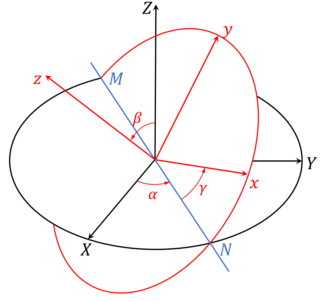
Figure 1: Euler angles $\alpha,\,\beta$ and $\gamma$ connecting the $X$-$Y$-$Z$ frame and the $x$-$y$-$z$ frame. The line $MN$ is the intersection of the $X$-$Y$ plane and the $x$-$y$ plane.

For a nonspherical star, the integral of the potential energy correction in Eq. (2) depends on the orientation of the star, causing a torque during its rotation. Specifically speaking, we calculate $\delta U$ in the body frame of the star at any instant,

$$\delta U=-\frac{1}{4}\bar{s}^{ij}\int d^{3}x\,d^{3}x^{\prime}\rho(\boldsymbol{x})\rho(\boldsymbol{x^{\prime}})\frac{\left(x^{i}-x^{\prime\,i}\right)\left(x^{j}-x^{\prime\,j}\right)}{|\boldsymbol{x}-\boldsymbol{x^{\prime}}|^{3}},$$ (6)

where $\rho$ is the density of the star, and is assumed to be independent of time in the body frame. The orientation dependence goes into $\delta U$ as the star rotates. If we set up an inertial frame $X$-$Y$-$Z$, then $\bar{s}^{ij}$ $(i,j=x,y,z)$ in the body frame is related to $\bar{s}^{IJ}$ $(I,J=X,Y,Z)$ in the inertial frame by a rotation transformation

$$\bar{s}^{ij}=R^{iI}R^{jJ}\bar{s}^{IJ}.$$ (7)

Noticing that $\bar{s}^{IJ}$ are the constant coefficients for Lorentz violation, $\delta U$ therefore depends on the orientation of the body through the rotation matrix $R^{iI}$. The orientation of the body is conveniently described by the Euler angles (see Fig. 1), which are the kinematic quantities to be solved from the equations of motion. For later use, we write the elements of the rotation matrix as

$$R^{iI}=\hat{\boldsymbol{e}}_{i}\cdot\hat{\boldsymbol{e}}_{I},$$ (8)

where $\{\hat{\boldsymbol{e}}_{i}\}$ $(i=x,y,z)$ is the basis of the body frame $x$-$y$-$z$, and $\{\hat{\boldsymbol{e}}_{I}\}$ $(I=X,Y,Z)$ is the basis of the inertial frame $X$-$Y$-$Z$. The inner products can be computed using the relations Landau and Lifshitz (1960)

$$\hat{\boldsymbol{e}}_{x} = \left(\cos\alpha\cos\gamma-\sin\alpha\cos\beta\sin\gamma\right)\hat{\boldsymbol{e}}_{X}$$

$$+\left(\sin\alpha\cos\gamma+\cos\alpha\cos\beta\sin\gamma\right)\hat{\boldsymbol{e}}_{Y}+\sin\beta\sin\gamma\,\hat{\boldsymbol{e}}_{Z},$$

$$\hat{\boldsymbol{e}}_{y} = \left(-\cos\alpha\sin\gamma-\sin\alpha\cos\beta\cos\gamma\right)\hat{\boldsymbol{e}}_{X}$$

$$+\left(-\sin\alpha\sin\gamma+\cos\alpha\cos\beta\cos\gamma\right)\hat{\boldsymbol{e}}_{Y}+\sin\beta\cos\gamma\,\hat{\boldsymbol{e}}_{Z},$$

$$\hat{\boldsymbol{e}}_{z} = \sin\alpha\sin\beta\,\hat{\boldsymbol{e}}_{X}-\cos\alpha\sin\beta\,\hat{\boldsymbol{e}}_{Y}+\cos\beta\,\hat{\boldsymbol{e}}_{Z}.$$ (9)

Back to the potential energy correction in Eq. (6), to proceed the calculation analytically as much as possible, we focus on the simple case where the star is a spheroid described by

$$\frac{x^{2}+y^{2}}{a_{1}^{2}}+\frac{z^{2}}{a_{3}^{2}}=1,$$ (10)

in the body frame and its density $\rho$ is axisymmetric about the $z$-axis (for an ellipsoid, see e.g., Ref. Xu et al. (2021)). In such case, one can show that $\bar{s}^{xy},\,\bar{s}^{xz}$ and $\bar{s}^{yz}$ do not appear in $\delta U$, and that $\bar{s}^{xx}$ and $\bar{s}^{yy}$ appear as the combination $\bar{s}^{xx}+\bar{s}^{yy}$. Because the trace $\bar{s}^{xx}+\bar{s}^{yy}+\bar{s}^{zz}$ is rotationally invariant and hence does not contribute to the anisotropic correction, the contribution from $\bar{s}^{xx}+\bar{s}^{yy}$ can be represented by $\bar{s}^{zz}$ so that the true anisotropic correction of the potential energy is simply

$$\delta U=C\,\bar{s}^{zz},$$ (11)

with the constant $C$ being

$$C=\frac{1}{4}\int d^{3}x\,d^{3}x^{\prime}\rho(\boldsymbol{x})\rho(\boldsymbol{x^{\prime}})\frac{\left(x-x^{\prime}\right)^{2}-\left(z-z^{\prime}\right)^{2}}{|\boldsymbol{x}-\boldsymbol{x^{\prime}}|^{3}}.$$ (12)

The result (11) deserves a comparison with that of Nordtvedt (1987). Treating the potential correction (4) as a perturbation on top of the Newtonian potential, Nordtvedt (1987) used the tensor virial relation to obtain the anisotropic gravitational self-energy for a spheroid star as

$$\delta U_{\rm PPN}=-\frac{1}{2}\alpha_{2}T_{\rm rot}(\boldsymbol{w}\cdot\hat{\boldsymbol{\Omega}})^{2},$$ (13)

where $T_{\rm rot}$ is the rotational kinetic energy and $\hat{\boldsymbol{\Omega}}$ is the unit vector along the angular velocity of the star.

First of all, we point out that with the replacement (5), Eq. (11) recovers the form of Eq. (13) when the star spins stationarily along the $z$-axis. As Nordtvedt obtained, for nonrelativistic stars, the constant $C$ is equal to $T_{\rm rot}/2$ by virtue of the tensor virial relation

$$K^{ij}+\delta^{ij}P-U^{ij}=0,$$ (14)

where $\delta^{ij}$ is the Kronecker delta, and

$$K^{ij} \equiv \int\rho v^{i}v^{j}d^{3}x,$$

$$P \equiv \int pd^{3}x,$$

$$U^{ij} \equiv \int\rho x^{i}\partial_{j}\Phi d^{3}x,$$ (15)

with ${\boldsymbol{v}}$ being the velocity field inside the star, $p$ being the pressure inside the star, and $\Phi$ being the usual Newtonian potential

$$\Phi({\boldsymbol{x}})=-\int d^{3}x^{\prime}\frac{\rho(\boldsymbol{x^{\prime}})}{|\boldsymbol{x}-\boldsymbol{x^{\prime}}|}.$$ (16)

The result $C=T_{\rm rot}/2$ is straightforward to prove once we notice the integral identity

$$U^{ij}=\frac{1}{2}\int d^{3}x\,d^{3}x^{\prime}\rho(\boldsymbol{x})\rho(\boldsymbol{x^{\prime}})\frac{\left(x^{i}-x^{\prime\,i}\right)\left(x^{j}-x^{\prime\,j}\right)}{|\boldsymbol{x}-\boldsymbol{x^{\prime}}|^{3}},$$ (17)

and for a star spinning along the $z$-direction,

$$K^{zz}=0,\quad T_{\rm rot}=\frac{1}{2}\left(K^{xx}+K^{yy}\right).$$ (18)

In Appendix A, the constant $C$ is exhibited for uniform spheroids by utilizing the Newtonian potential inside an ellipsoid of uniform density (see e.g., Refs. Poisson and Will (2014); Chandrasekhar and Lebovitz (1962)).

Secondly, we notice that Eq. (11) and Eq. (13) are different for a generally rotating spheroidal star whose angular velocity is not aligned with its symmetric axis. The origin of the difference is that Eq. (13) requires the star to be a stationary fluid in equilibrium while Eq. (11) applies as long as the star has an axisymmetric mass distribution. Whether the star is a fluid or a rigid body does not affect the validity of Eq. (11). Now comes the question: How could the state of the star influence the alignment between its angular velocity and symmetric axis? In fact, if the star is a rigid body, then the direction of its angular velocity can be different from its symmetric axis. But when it is a fluid, the deformation is caused by rotation, and therefore its symmetric axis must be aligned with its angular velocity as long as the system is in equilibrium.

To better understand the context and the limitation for Eq. (13), let us consider a freely rotating star, namely when there is no torque. If modeled as a rigid body, depending on whether the angular velocity is aligned with the symmetric axis, two kinds of solution exist: the stationary spinning solution where the star spins around the fixed symmetric axis, and the free-precessing solution where the star spins around its symmetric axis while that axis rotates around the fixed direction of the conserved angular momentum Landau and Lifshitz (1960). If modeled as a fluid, the free-precessing solution cannot exist because even if the angular velocity is not aligned with the symmetric axis initially, the deformation caused by rotation will eventually change the symmetric axis to the direction of angular velocity, leaving the star in the state of stationary spin.

When the torque caused by Lorentz violation is taken into consideration, the two types of solution for a freely rotating star, namely the stationary spinning solution and the free-precessing solution, might be treated as the zeroth-order solution for applying perturbation method. The details are discussed in Sec. II.2. Here we just point out that the effect of the Lorentz-violating torque is forcing the star to precess around one of the principal axes of the $\bar{s}^{ij}$ tensor. When this effect is added to a stationary spinning star, we call the motion single precession. When the forced precession due to Lorentz violation is added to a free-precessing star, we call the motion twofold precession.

In the single-precession solution, the precession is caused by Lorentz violation, which is assumed to be small. Therefore, the total angular velocity can be approximated as aligned with the symmetric axis of the star. This enables us to put Eq. (11) in the form of Eq. (13) at the leading order of Lorentz violation via the replacement (5). So the single-precession solution is the one found by Nordtvedt (1987). However, for our result, there is no need to restrict it to fluid stars as Eq. (11) applies to fluids as well as rigid bodies. The other solution that we defined, the twofold-precession solution, as its name suggests, is a superposition of the free precession where the symmetric axis of the star precesses around the angular momentum, and the forced precession where the angular momentum precesses around one of the principal axes of the $\bar{s}^{ij}$ tensor. Though only applicable to stars if they are modeled as rigid bodies, the twofold-precession solution describes a new Lorentz-violating effect in the rotation of stars that has not been studied in the literature to our knowledge.

Before moving to study the solutions in detail, a brief clarification on the model of NS deformation might be useful. We will adopt the model described by Jones and Andersson (2001) where the deformation of the star has two contributions: the centrifugal deformation and the Coulomb deformation. The centrifugal deformation is the fluid deformation that scales with the square of the angular velocity, while the Coulomb deformation describes the rigid deviation from the spherical shape sustained by the electrostatic force. The fact that the electrostatic interaction is much weaker than the gravitational interaction in NSs implies that the rigid Coulomb deformation is much smaller than the fluid centrifugal deformation. Using the oblateness defined as

$$\epsilon=\frac{I^{zz}-I^{xx}}{I^{xx}},$$ (19)

where $I^{xx}$ and $I^{zz}$ are the eigenvalues of the moment of inertia tensor, to characterize the deformations of spheroidal stars, an estimation for the centrifugal deformation is

$$\epsilon_{f}\approx\frac{|{\boldsymbol{\Omega}}|^{2}R^{3}}{M}\approx 2.1\times 10^{-3}\left(\frac{{|{\boldsymbol{\Omega}}|}/{2\pi}}{100\,{\rm Hz}}\right)^{2}\left(\frac{R}{10\,{\rm km}}\right)^{3}\left(\frac{1.4M_{\odot}}{M}\right),$$ (20)

where ${\boldsymbol{\Omega}}$ is the angular velocity, $R$ is the radius, and $M$ is the mass of the NS, while the oblateness $\epsilon_{r}$ caused by the Coulomb deformation is about five orders of magnitude smaller Jones and Andersson (2001). Therefore, when applying the single-precession solution to NSs, the rigid deformation $\epsilon_{r}$ can be neglected and the deformation is described by the fluid oblateness $\epsilon_{f}$. However, the fact that NSs can have rigid deformation described by $\epsilon_{r}$ is vital when the twofold-precession solution is to apply. Similar to the free-precessing NSs considered in Refs. Zimmermann and Szedenits (1979); Jones and Andersson (2001); Gao et al. (2020); Gao and Shao (2020), NSs with Lorentz-violating gravity under the twofold precession produce modulated pulsar signals and in the meantime are sources of continuous GWs, providing potential new tests of Lorentz violation. This will be the central topic in Sec. III.

Finally, we point out that Lorentz violation itself also deforms stars Altschul (2007); Xu et al. (2020). But then the deformation due to Lorentz violation contributes at the second order in terms of the coefficients for Lorentz violation to the anisotropic gravitational self-energy. To keep the analysis clear and tractable, we neglect any Lorentz-violating correction to the structure of stars in this work.

II.2 Rotation of a spheroidal star

We are ready to write down the equations of motion and solve the rotation of a spheroidal star. First, the coefficients for Lorentz violation naturally fix a convenient inertial frame, namely the one that diagonalizes the $\bar{s}^{IJ}$ matrix. We will use it as the inertial frame $X$-$Y$-$Z$. Please note that the inertial frame widely used in the literature is the canonical Sun-centered celestial-equatorial frame Kostelecký and Mewes (2002). It is generally different from the frame used here as the off-diagonal coefficients for Lorentz violation unlikely happen to vanish in the canonical Sun-centered celestial-equatorial frame.

With the rotation matrix (8), the anisotropic gravitational self-energy (11) is

$$\delta U=C\left((\bar{s}^{XX}\sin^{2}\alpha+\bar{s}^{YY}\cos^{2}\alpha)\sin^{2}\beta+\bar{s}^{ZZ}\cos^{2}\beta\right),$$ (21)

where $\bar{s}^{XX},\,\bar{s}^{YY}$, and $\bar{s}^{ZZ}$ are the eigenvalues of the $\bar{s}^{IJ}$ matrix. Then, to express the rotational kinetic energy in terms of the Euler angles and their derivatives, we employ the kinematic relation between the velocity components in the body frame and the Euler angles Landau and Lifshitz (1960),

$$\Omega^{x} = \dot{\alpha}\sin\beta\sin\gamma+\dot{\beta}\cos\gamma,$$

$$\Omega^{y} = \dot{\alpha}\sin\beta\cos\gamma-\dot{\beta}\sin\gamma,$$

$$\Omega^{z} = \dot{\alpha}\cos\beta+\dot{\gamma},$$ (22)

where dot denotes time derivative. With $I^{xx}=I^{yy}$, the rotational kinetic energy simplifies to

$$T_{\rm rot}=\frac{1}{2}I^{xx}\left(\dot{\alpha}^{2}\sin^{2}\beta+\dot{\beta}^{2}\right)+\frac{1}{2}I^{zz}\left(\dot{\alpha}\cos\beta+\dot{\gamma}\right)^{2}.$$ (23)

The Euler-Lagrange equations from $L=T_{\rm rot}-\delta U$ can be derived, and there are two first integrals,

$$E = T_{\rm rot}+\delta U,$$

$$\Omega^{z} = \dot{\alpha}\cos\beta+\dot{\gamma}.$$ (24)

The total energy $E$ is not much useful in helping simplify the other equations. The $z$-component of the angular velocity, $\Omega^{z}$, can be used to eliminate $\dot{\gamma}$ from the other two Euler-Lagrange equations so that they become

$$\sin^{2}\beta\,\ddot{\alpha}+\sin{2\beta}\,\dot{\alpha}\dot{\beta}-\frac{I^{zz}\Omega^{z}}{I^{xx}}\sin\beta\,\dot{\beta} = -\frac{1}{I^{xx}}\frac{\partial\delta U}{\partial\alpha},$$

$$\ddot{\beta}-\frac{1}{2}\sin{2\beta}\,\dot{\alpha}^{2}+\frac{I^{zz}\Omega^{z}}{I^{xx}}\sin\beta\,\dot{\alpha} = -\frac{1}{I^{xx}}\frac{\partial\delta U}{\partial\beta}.$$ (25)

First, we consider an illustrative case where only $\bar{s}^{ZZ}$ is nonzero. This is the case where the tensor $\bar{s}^{ij}$ degenerates to a vector as in the correspondence (5). With $\bar{s}^{XX}=\bar{s}^{YY}=0$, $\delta U$ is independent of $\alpha$ so that solutions with $\ddot{\alpha}=0,\,\dot{\beta}=0$ are consistent with Eqs. (25) given

$$\dot{\alpha}=\frac{I^{zz}\Omega^{z}\pm\sqrt{\left(I^{zz}\Omega^{z}\right)^{2}-8\bar{s}^{ZZ}CI^{xx}\cos^{2}\beta}}{2I^{xx}\cos\beta}.$$ (26)

When $\bar{s}^{ZZ}=0$, the “$+$” sign recovers the free-precessing solution and the “$-$” sign gives the stationary spinning solution. Correspondingly, for $\bar{s}^{ZZ}\neq 0$, the “$+$” sign gives what we call twofold precession, and the “$-$” sign gives what we call single precession. The single-precession solution, once approximated at the leading order of $\bar{s}^{ZZ}\leftrightarrow-\alpha_{2}|\boldsymbol{w}|^{2}$, is the one obtained by Nordtvedt (1987).

The solutions (26) hold when the matrix $\bar{s}^{IJ}$ has only one nonvanishing eigenvalue whose eigenvector is chosen to be the $Z$-axis. Similar solutions exist when the matrix $\bar{s}^{IJ}$ has two same eigenvalues whose eigenvectors are chosen to be the $X$-axis and the $Y$-axis, because in such case $\delta U$ is also independent of $\alpha$. In fact, only one nonvanishing eigenvalue is a special case of two same eigenvalues where the same eigenvalues are zero. In conclusion, when the matrix $\bar{s}^{IJ}$ has two same eigenvalues, we can set up the $X$-$Y$-$Z$ frame properly so that solutions similar to Eq. (26) with a constant $\beta$ exist.

Now we can discuss the solutions in general when the matrix $\bar{s}^{IJ}$ has three different eigenvalues. In such case, $\delta U$ depends on both $\alpha$ and $\beta$. Solutions with a constant $\beta$ do not exist, but as Lorentz violation is supposed to be small, we use the ansatz

$$\alpha = \alpha_{0}+at+\alpha^{(1)},$$

$$\beta = \beta_{0}+\beta^{(1)},$$ (27)

to find perturbative solutions at the leading order of Lorentz violation. In the ansatz (27), $\alpha_{0}$ and $\beta_{0}$ are constants, while $\alpha^{(1)}$ and $\beta^{(1)}$ are functions of time assumed to be much smaller than 1. The constant $a$, representing the precessing angular velocity for free rotation, takes the values

$$a=\begin{cases}\frac{\omega}{\cos\beta_{0}},&{\rm free\ precession},\\ 0,&{\rm stationary\ spin},\end{cases}$$ (28)

with $\omega\equiv I^{zz}\Omega^{z}/I^{xx}$ according to Eq. (26) when $\bar{s}^{ZZ}=0$. Substituting derivatives of the ansatz (27) into Eqs. (25), and approximating $\alpha$ and $\beta$ in the equations with $\alpha_{0}+at$ and $\beta_{0}$, we find

$$\ddot{\alpha}^{(1)}\pm\frac{\omega}{\sin\beta_{0}}\,\dot{\beta}^{(1)} = -\frac{1}{I^{xx}\sin^{2}\beta_{0}}\frac{\partial\delta U}{\partial\alpha}\Big{|}_{\alpha=\alpha_{0}+at,\,\beta=\beta_{0}},$$

$$\ddot{\beta}^{(1)}\mp\omega\sin\beta_{0}\,\dot{\alpha}^{(1)} = -\frac{1}{I^{xx}}\frac{\partial\delta U}{\partial\beta}\Big{|}_{\alpha=\alpha_{0}+at,\,\beta=\beta_{0}}.$$ (29)

Note that the upper signs are for the perturbation to a free-precessing star, generating twofold-precession solutions, while the lower signs are for the perturbation to a stationary spinning star, generating single-precession solutions. We will stick to this sign convention when we write expressions containing upper and lower signs. Equations (29) are two coupled oscillation equations for $\dot{\alpha}^{(1)}$ and $\dot{\beta}^{(1)}$ with driven forces. Using Eq. (21) to write out the right-hand sides of Eqs. (29), the solutions can be found as

$$\dot{\alpha}^{(1)} = \mp a^{(1)}\mp\frac{A}{\sin\beta_{0}}\sin{(\omega t+\varphi)}+\eta_{\alpha}\,\tilde{C}\cos{2(at+\alpha_{0})},$$

$$\dot{\beta}^{(1)} = A\cos{(\omega t+\varphi)}+\eta_{\beta}\,\tilde{C}\sin{2(at+\alpha_{0})},$$ (30)

with $A$ and $\varphi$ being two integral constants of the homogeneous solutions. The constants $a^{(1)},\,\tilde{C},\,\eta_{\alpha}$, and $\eta_{\beta}$ are

$$a^{(1)} = \frac{C\left(2\bar{s}^{ZZ}-\bar{s}^{XX}-\bar{s}^{YY}\right)\cos\beta_{0}}{I^{zz}\Omega^{z}},$$

$$\tilde{C} = \frac{C\left(\bar{s}^{XX}-\bar{s}^{YY}\right)}{I^{zz}\Omega^{z}},$$

$$\eta_{\alpha} = \begin{cases}\frac{\cos\beta_{0}\left(2+\cos^{2}\beta_{0}\right)}{4-\cos^{2}\beta_{0}},&{\rm twofold\ precession},\\ \cos\beta_{0},&{\rm single\ precession},\end{cases}$$

$$\eta_{\beta} = \begin{cases}\frac{3\sin\beta_{0}\cos^{2}\beta_{0}}{4-\cos^{2}\beta_{0}},&~{}~{}~{}~{}{\rm twofold\ precession},\\ \sin\beta_{0},&~{}~{}~{}~{}{\rm single\ precession}.\end{cases}$$ (31)

We point out that when $\bar{s}^{XX}=\bar{s}^{YY}=0$, the inhomogeneous solutions in Eqs. (30) recover the solutions (26) at the leading order of Lorentz violation.

The constant $a^{(1)}$, generated by the constant term on the right-hand side of the second equation in Eqs. (29), represents the forced precession due to Lorentz violation. It can be absorbed into $a$ by redefining $a$ to be

$$a=\begin{cases}\frac{\omega}{\cos\beta_{0}}-a^{(1)},&{\rm twofold\ precession},\\ a^{(1)},&{\rm single\ precession}.\end{cases}$$ (32)

Note that the forced precession acts oppositely on a free-precessing star and a stationary spinning star.

Now we can use this new $a$ in solutions (30), and the benefit is that the second term in $\dot{\beta}^{(1)}$ is no longer constant for the single-precession solution. As $\beta$ at most changes from $0$ to $\pi$ by definition, its rate of change really should not contain any constant term. Keeping in mind that the definition (32) is used, then the ansatz (27), together with the solutions for $\alpha^{(1)}$ and $\beta^{(1)}$,

$$\alpha^{(1)} = \pm\frac{A}{\omega\sin\beta_{0}}\cos{(\omega t+\varphi)}+\eta_{\alpha}\frac{\tilde{C}}{2a}\sin{2(at+\alpha_{0})},$$

$$\beta^{(1)} = \frac{A}{\omega}\sin{(\omega t+\varphi)}-\eta_{\beta}\frac{\tilde{C}}{2a}\cos{2(at+\alpha_{0})},$$ (33)

gives the perturbation solutions with integral constants $A,\,\varphi,\,\alpha_{0}$, and $\beta_{0}$.

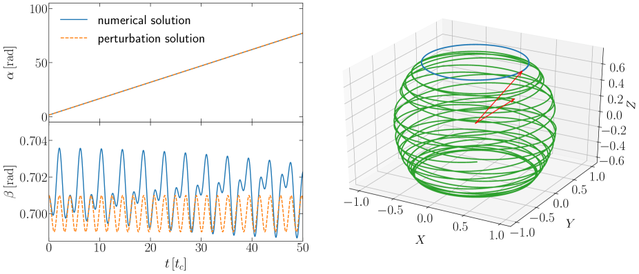
Figure 2: Example I of twofold precession (denoted as tp-I hereafter). The left plots are the solutions of the Euler angles $\alpha$ and $\beta$ as functions of time. The right plot shows the trajectories of the heads of $\hat{\boldsymbol{e}}_{x}$ (green) and $\hat{\boldsymbol{e}}_{z}$ (blue) in the $X$-$Y$-$Z$ frame while their tails are fixed at the origin. The arrows mark the two vectors at $t=0$. The initial values, $\alpha|_{t=0}=\frac{\pi}{2}$, $\beta|_{t=0}\approx 0.701$, $\dot{\alpha}|_{t=0}\approx 1.509$, and $\dot{\beta}|_{t=0}=0$ are adopted by setting $\alpha_{0}=\frac{\pi}{2}$, $\beta_{0}=0.7$, $A=0$, and $\varphi=\frac{\pi}{2}$ in Eqs. (34). Other parameters used are $\gamma|_{t=0}=0$, $\Omega^{z}=1$, $I^{zz}/I^{xx}=1.1$, and $\left\{\bar{s}^{XX},\bar{s}^{YY},\bar{s}^{ZZ}\right\}=\{0.02,0.01,-0.04\}$. Time and time derivatives are dimensionless under the time unit $t_{c}$ defined in Eq. (35).

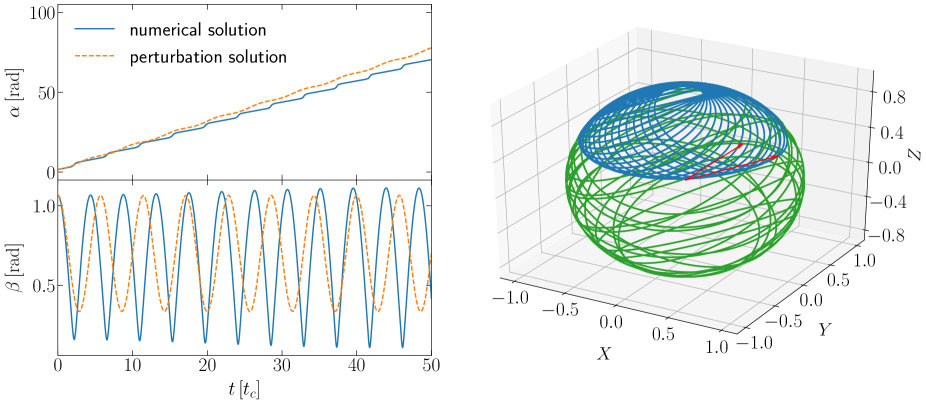
Figure 3: Example II of twofold precession (denoted as tp-II hereafter). See the caption of Fig. 2 for the meaning of illustration. The initial values, $\alpha|_{t=0}=\frac{\pi}{2}$, $\beta|_{t=0}\approx 1.065$, $\dot{\alpha}|_{t=0}\approx 0.889$, and $\dot{\beta}|_{t=0}=0$ are adopted by setting $\alpha_{0}=\frac{\pi}{2}$, $\beta_{0}=0.7$, $A=0.4$, and $\varphi=\frac{\pi}{2}$ in Eqs. (34). Other parameters are the same as those in Fig. 2.

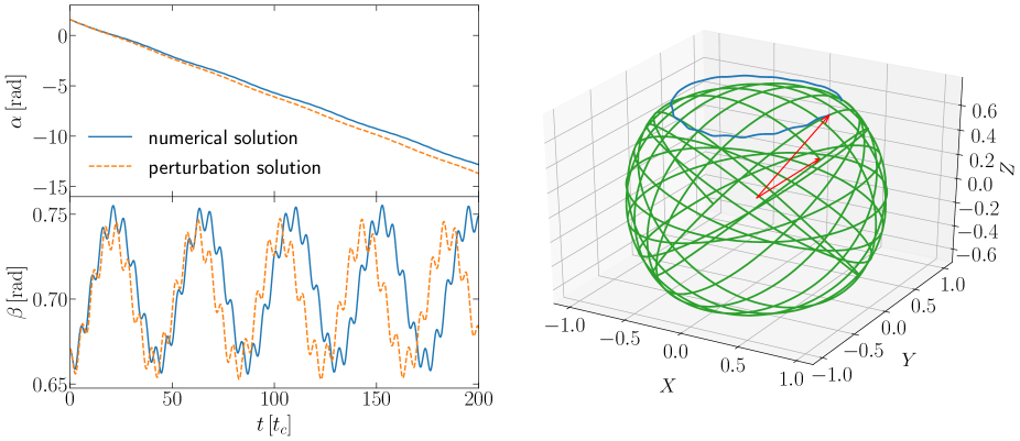
Figure 4: Example I of single precession. See the caption of Fig. 2 for the meaning of illustration. The initial values, $\alpha|_{t=0}=\frac{\pi}{2}$, $\beta|_{t=0}\approx 0.671$, $\dot{\alpha}|_{t=0}\approx-0.068$, and $\dot{\beta}|_{t=0}=0$ are adopted by setting $\alpha_{0}=\frac{\pi}{2}$, $\beta_{0}=0.7$, $A=0.01$, and $\varphi=\frac{\pi}{2}$ in Eqs. (34). Other parameters are the same as those in Fig. 2.

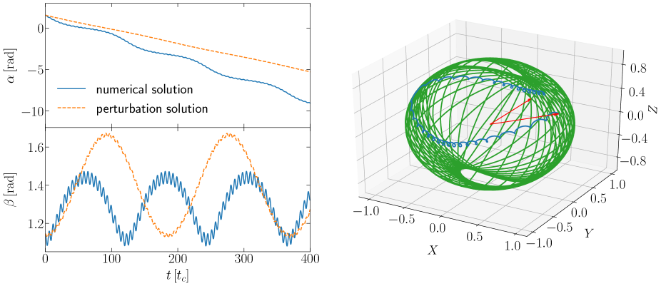
Figure 5: Example II of single precession. See the caption of Fig. 2 for the meaning of illustration. The initial values, $\alpha|_{t=0}=\frac{\pi}{2}$, $\beta|_{t=0}\approx 1.146$, $\dot{\alpha}|_{t=0}\approx-0.008$, and $\dot{\beta}|_{t=0}=0$ are adopted by setting $\alpha_{0}=\frac{\pi}{2}$, $\beta_{0}=1.4$, $A=0.01$, and $\varphi=\frac{\pi}{2}$ in Eqs. (34). Other parameters are the same as those in Fig. 2.

The perturbation solutions are useful in analytically illustrating how Lorentz violation described by the matrix $\bar{s}^{IJ}$ with three different eigenvalues affects a freely rotating spheroidal star. But a complete discussion of the rotational motion has to involve numerical solutions, because there are solutions to Eqs. (25) unable to be described by the perturbation solutions even at the leading order of Lorentz violation. To see this, let us consider solving Eqs. (25) with initial values given by

$$\alpha|_{t=0} = \alpha_{0}\pm\frac{A}{\omega\sin\beta_{0}}\cos{\varphi}+\eta_{\alpha}\frac{\tilde{C}}{2a}\sin{2\alpha_{0}},$$

$$\beta|_{t=0} = \beta_{0}+\frac{A}{\omega}\sin{\varphi}-\eta_{\beta}\frac{\tilde{C}}{2a}\cos{2\alpha_{0}},$$

$$\dot{\alpha}|_{t=0} = a\mp\frac{A}{\sin\beta_{0}}\sin{\varphi}+\eta_{\alpha}\tilde{C}\cos{2\alpha_{0}},$$

$$\dot{\beta}|_{t=0} = A\cos\varphi+\eta_{\beta}\tilde{C}\sin{2\alpha_{0}}.$$ (34)

The fact that the initial values $\alpha|_{t=0}$, $\beta|_{t=0}$, $\dot{\alpha}|_{t=0}$, and $\dot{\beta}|_{t=0}$ might be arbitrarily assigned indicates that the corresponding integral constants $A,\,\varphi,\,\alpha_{0}$, and $\beta_{0}$ should also be able to take any values. However, the perturbative approach restricts $A$ to be small, losing solutions where $\dot{\alpha}|_{t=0}$ is at the order of $\omega/\cos\beta_{0}$ but significantly different from it. These solutions belong to the case of twofold precession, but because the directions of angular momentum around which free precession happens deviate from the $Z$-axis too much, free precession around the $Z$-axis is no longer able to serve as the zeroth-order solution for the perturbation method. More seriously, the perturbative approach assumes $\alpha^{(1)}$ and $\beta^{(1)}$ to be much smaller than 1. But for the single-precession solution in Eqs. (33), this assumption is very much questionable as a small quantity $a=a^{(1)}$ appears in the denominators of the second terms of $\alpha^{(1)}$ and $\beta^{(1)}$. Somehow the perturbative single-precession solution does mimic numerical solutions in one period of the forced precession when $\beta_{0}$ is small ($\beta_{0}\mathrel{\hbox to0.0pt{\lower 4.0pt\hbox{\hskip 1.0pt$\sim$}\hss}\raise 1.0pt\hbox{$<$}}1$). But when $\beta_{0}$ gets close to $\pi/2$, the approximation fails completely.

Figures 2–5 display examples to compare the perturbation solutions with numerical solutions, and also illustrate the cases where perturbation method is invalid. In the figures the time and angular velocities have dimensionless values by employing a time unit $t_{c}$ defined as

$$t_{c}=\sqrt{\frac{I^{xx}}{C}}.$$ (35)

Then, for demonstrating purpose, the integral constant $\Omega^{z}$ is taken to be 1, the ratio $I^{zz}/I^{xx}$ is taken to be 1.1, and the eigenvalues of $\bar{s}^{ij}$ are taken to be $\bar{s}^{XX}=0.02,\,\bar{s}^{YY}=0.01,\,\bar{s}^{ZZ}=-0.04$.

Before turn to observational consequences, let us address the fact that our discussion above assumes that the forced precession due to Lorentz violation is around the $Z$-axis. Depending on the initial values, the forced precession can be around the other two principal axes of the matrix $\bar{s}^{IJ}$. An interesting result from our study of the numerical solutions is that without loss of generality, if the three different eigenvalues of $\bar{s}^{ij}$ satisfy $\bar{s}^{ZZ}<\bar{s}^{YY}<\bar{s}^{XX}$, then the forced precession around the $Y$-axis is unstable. This is very similar to the Dzhanibekov effect (also called the tennis racket theorem) in free rotation Poinsot (1851). Once this is stated, we point out that the above discussion equally applies to the forced precession around the $X$-axis by changing the indices

$$Z\rightarrow X,\quad X\rightarrow Y,\quad Y\rightarrow Z,$$ (36)

in Eqs. (31) and keeping in mind that $(\alpha,\beta,\gamma)$ now refer to the Euler angles between the $x$-$y$-$z$ frame and the $Y$-$Z$-$X$ frame (see Fig. 6).

III observational consequences

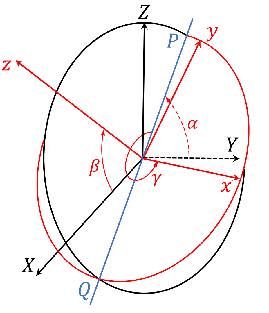
Figure 6: Euler angles $\alpha,\,\beta$, and $\gamma$ connecting the $Y$-$Z$-$X$ frame and the $x$-$y$-$z$ frame. The line $PQ$ is the intersection of the $Y$-$Z$ plane and the $x$-$y$ plane.

NSs observed as pulsars provide tests against the above predicted single-precession motion due to Lorentz-violating gravity Nordtvedt (1987); Shao et al. (2013); Shao (2014, 2020). In Sec. III.1 we will discuss constraints set on the coefficients for Lorentz violation by applying the single-precession solution to two observed solitary millisecond pulsars Shao et al. (2013). On the other hand, the twofold-precession solution, developed from free precession once Lorentz-violating gravity presents, has not found its tests as evidences of free-precessing NSs are yet preliminary (see e.g. Ref. Stairs et al. (2000)). Based on the hypothesis that NSs might possess tiny rigid deformation, the modulations on pulsar signals and the emission of continuous GWs due to free precession have been studied in the literature to predict observational signatures for searching such NSs Zimmermann and Szedenits (1979); Jones and Andersson (2001); Gao et al. (2020); Gao and Shao (2020). Following similar considerations, we investigate in Secs. III.2 and III.3 observational signatures in pulsar pulses and continuous GW signals from NSs undergoing the twofold-precession motion.

III.1 Single-precession motion and constraints on Lorentz violation

We start with considering the change of the angle between the spin axis $\hat{\boldsymbol{e}}_{z}$ and a fixed direction in the $X$-$Y$-$Z$ frame when a star is in the state of single precession. Calling that angle $\lambda$ and describing the fixed direction using the spherical angular coordinates $(\theta_{o},\,\phi_{o})$ in the $X$-$Y$-$Z$ frame, we have the relation

$$\cos\lambda = \sin\theta_{o}\sin\beta\sin{(\alpha-\phi_{o})}+\cos\theta_{o}\cos\beta,$$ (37)

where $\alpha$ and $\beta$ are Euler angles used in Sec. II. Assume that the changes in $\alpha$ and $\beta$ are much smaller than 1 during a certain time interval, then the change of $\cos\lambda$ can be approximated as

$$\Delta\cos\lambda \approx \left(\sin\theta_{o}\cos\beta\sin{(\alpha-\phi_{o})}-\cos\theta_{o}\sin\beta\right)\Delta\beta$$ (38)

$$+\sin\theta_{o}\sin\beta\cos{(\alpha-\phi_{o})}\Delta\alpha.$$

For estimations, we use the perturbation solution (27) to approximate the changes in $\alpha$ and $\beta$ as

$$\Delta\alpha \approx \dot{\alpha}\Delta t=\left(1+\frac{A}{a^{(1)}\sin\beta_{0}}\sin{\varphi}+\frac{\cos\beta_{0}\tilde{C}}{a^{(1)}}\cos{2\alpha_{0}}\right)a^{(1)}\Delta t,$$

$$\Delta\beta \approx \dot{\beta}\Delta t=\left(\frac{A}{a^{(1)}}\cos{\varphi}+\frac{\sin\beta_{0}\tilde{C}}{a^{(1)}}\sin{2\alpha_{0}}\right)a^{(1)}\Delta t,$$ (39)

where the start of the time interval $\Delta t$ has been set at $t=0$. Because $A,\,\tilde{C}$, and $a^{(1)}$ are at the same order, $\Delta\alpha,\,\Delta\beta$, and hence $\Delta\cos\lambda$ are proportional to $a^{(1)}\Delta t$ with factors of order unity. Here we neglect any situation where $(\theta_{o},\,\phi_{o})$ and $\{A,\,\varphi,\,\alpha_{0},\,\beta_{0}\}$ are fine-tuned to vanish the factor for $\Delta\cos\lambda$. Once an observation puts a bound on the change of $\lambda$ during a certain time interval, corresponding constraints on the combination $2\bar{s}^{ZZ}-\bar{s}^{XX}-\bar{s}^{YY}$ is

$$\left|2\bar{s}^{ZZ}-\bar{s}^{XX}-\bar{s}^{YY}\right|\lesssim\left|\frac{I^{zz}\Omega^{z}}{C\Delta t\cos\beta_{0}}\,\Delta\cos\lambda\right|.$$ (40)

The estimation (40) depends on $\beta_{0}$, which roughly characterizes the angle between the symmetric axis of the star and the Lorentz-violating principal axis around which the forced precession happens. Checked with numerical results, we find that when $\beta_{0}\lesssim 1.1$, the estimation (40) gives correct orders of magnitude for $\left|2\bar{s}^{ZZ}-\bar{s}^{XX}-\bar{s}^{YY}\right|$. But as we mentioned in Sec. II.2, when $\beta_{0}$ approaches $\pi/2$, the estimation (40) fails because the perturbation method breaks down. A semianalytical relation based on Eq. (40) and numerical results is

$$\left|2\bar{s}^{ZZ}-\bar{s}^{XX}-\bar{s}^{YY}\right|\lesssim\eta\left|\frac{I^{zz}\Omega^{z}}{C\Delta t}\,\Delta\cos\lambda\right|,$$ (41)

where $\eta$ can be approximated by $1/\cos\beta_{0}$ for $\beta_{0}\lesssim 1.1$ but then only increases to $10$ when $\beta_{0}$ approaches $\pi/2$.

Table 1: Observational quantities from PSRs B1937+21 and J1744$-$1134 Shao et al. (2013) to constrain Lorentz violation. The pulse profile of PSR B1937+21 consists of a main pulse and an interpulse, both of which put bounds on the change of $\lambda$ and hence constrain Lorentz violation. The pulse width is taken at $50\%$ intense level in practice. The last row, conservative bound on $\left|2\bar{s}^{ZZ}-\bar{s}^{XX}-\bar{s}^{YY}\right|$, is obtained by setting $\eta=10$.

	Main pulse of PSR B1937+21	Interpulse of PSR B1937+21	PSR J1744$-$1134
Spin period (ms)	$1.6$	$1.6$	$4.1$
$W$ (deg)	$8.3$	$10$	$13$
Bound on $\Delta W$ ($10^{-3}$ deg)	$-48$	$53$	$20$
$\lambda$ (deg)	$100$	$100$	$95$
$\chi$ (deg)	75	$105$	51
Bound on $\Delta\lambda$ ($10^{-3}$ deg)	$-19$	$-5.2$	1.6
Bound on $\left|2\bar{s}^{ZZ}-\bar{s}^{XX}-\bar{s}^{YY}\right|$	$10^{-14}\eta$	$10^{-15}\eta$	$10^{-16}\eta$
Conservative bound on $\left|2\bar{s}^{ZZ}-\bar{s}^{XX}-\bar{s}^{YY}\right|$	$10^{-13}$	$10^{-14}$	$10^{-15}$

Now we are ready to apply Eq. (41) to two solitary pulsars: PSRs B1937+21 and J1744$-$1134. Their observed pulse profiles over 15 years were thoroughly analyzed by Shao et al. (2013). Here we simply use the conclusion that the change in the angle $\lambda$, now being the angle between the spin axis and the line of sight, is bounded by

$$\Delta\lambda=\frac{1}{2}\frac{\sin{\frac{W}{2}}}{\cot\lambda\cos{\frac{W}{2}}+\cot\chi}\,\Delta W,$$ (42)

where $W$ is the pulse width, $\Delta W$ is the change in $W$ during the 15 years, and $\chi$ is the angle between the spin axis of the NS and the symmetric axis of the pulsar beam which has been assumed to take the shape of a narrow cone Lorimer and Kramer (2005). The values of those quantities for each pulsar are listed in Table 1. The derived bounds on $\Delta\lambda$ and hence on the combination $\left|2\bar{s}^{ZZ}-\bar{s}^{XX}-\bar{s}^{YY}\right|$ are shown in the last three rows of the table (the last row is the same as the last second row except that $\eta$ is set to $10$, which is suggested as the upper limit of $\eta$ by our numerical solutions). As an estimation, a uniform density of $\rho_{\rm NS}\sim 10^{15}{\rm g}/{\rm cm}^{3}$ and a fluid deformation of $\epsilon_{f}\sim 10^{-3}$ have been used to get

$$\frac{I^{zz}}{C}\approx\frac{15}{4\pi}\frac{1}{\rho_{\rm NS}\epsilon_{f}}\sim 10^{-5}\,{\rm s}^{2},$$ (43)

for the NSs.

Under the correspondence (5), the constraints in Table 1 are consistent with those in Ref. Shao et al. (2013) for the PPN $\alpha_{2}$ parameter. Then we do notice that they are 3 to 5 orders of magnitude better than the global results in Ref. Shao (2014) where the same two solitary pulsars were used but the test was done together with another 11 binary pulsars in order to obtain global constraints on the coefficients for Lorentz violation instead of the “maximal-reach” ones as is done here Tasson (2020). This shows that, (i) observations of solitary pulsars are more sensitive to Lorentz violation than those of binary pulsars, and (ii) the correlations between different coefficients for Lorentz violation can severely degrade the constraints Shao (2014).

III.2 Twofold-precession motion and pulsar signal

To construct pulsar signals from a NS under the twofold-precession motion, we adopt the cone model to describe the radiation beam Gil et al. (1984); Lorimer and Kramer (2005). Figure 7 illustrates a half radiation cone in the $X$-$Y$-$Z$ frame. In principle, the radiation comes from two opposite sides of a NS and is in the shape of a doule cone. But for clarity, we will only track the half cone as shown in Fig. 7 and analyze the signal from it. The signal from the opposite half cone can be obtained simply by reversing the unit vector along the axis of the cone in the following analysis.

In the cone model, signals are observed when the line of sight is inside the radiation cone. Mathematically, it means

$$\cos\rho<\hat{\boldsymbol{m}}\cdot\hat{\boldsymbol{n}},$$ (44)

where $\rho$ is the semi-open angle of the cone, $\hat{\boldsymbol{m}}$ is the unit vector along the axis of the cone, and $\hat{\boldsymbol{n}}$ is the unit vector along the line of sight. The axis of the cone, generally believed to be aligned with the magnetic dipole moment of the star, is fixed in the body frame and therefore can be described by two constant angular coordinates $(\chi,\delta)$ as

$$\hat{\boldsymbol{m}}=\sin\chi\cos\delta\,\hat{\boldsymbol{e}}_{x}+\sin\chi\sin\delta\,\hat{\boldsymbol{e}}_{y}+\cos\chi\,\hat{\boldsymbol{e}}_{z}.$$ (45)

The direction of the line of sight, if we neglect the proper motion of the star relative to the observer, is fixed in the $X$-$Y$-$Z$ frame and will be described by two constant angular coordinates $(\theta_{o},\phi_{o})$ as

$$\hat{\boldsymbol{n}}=\sin\theta_{o}\cos\phi_{o}\,\hat{\boldsymbol{e}}_{X}+\sin\theta_{o}\sin\phi_{o}\,\hat{\boldsymbol{e}}_{Y}+\cos\theta_{o}\,\hat{\boldsymbol{e}}_{Z}.$$ (46)

Using Eqs. (9), the product of $\hat{\boldsymbol{m}}$ and $\hat{\boldsymbol{n}}$ can be written as a function of time due to the time-dependent Euler angles,

$$\hat{\boldsymbol{m}}\cdot\hat{\boldsymbol{n}} = \sin\theta_{o}\sin\chi\cos{(\alpha-\phi_{o})}\cos{(\gamma+\delta)}$$ (47)

$$-\sin\theta_{o}\sin\chi\sin{(\alpha-\phi_{o})}\cos\beta\sin{(\gamma+\delta)}$$

$$+\cos\theta_{o}\cos\chi\cos\beta$$

$$+\sin\theta_{o}\cos\chi\sin{(\alpha-\phi_{o})}\sin\beta$$

$$+\cos\theta_{o}\sin\chi\sin\beta\sin{(\gamma+\delta)}.$$

The angles $\phi_{o}$ and $\delta$ can be absorbed into the initial values of $\alpha$ and $\gamma$ in the above expression. For given $\theta_{o},\,\chi$, and $\rho$, once the rotation of the star is known, the inequality (44) can be solved to predict the time intervals during which signals are observed.

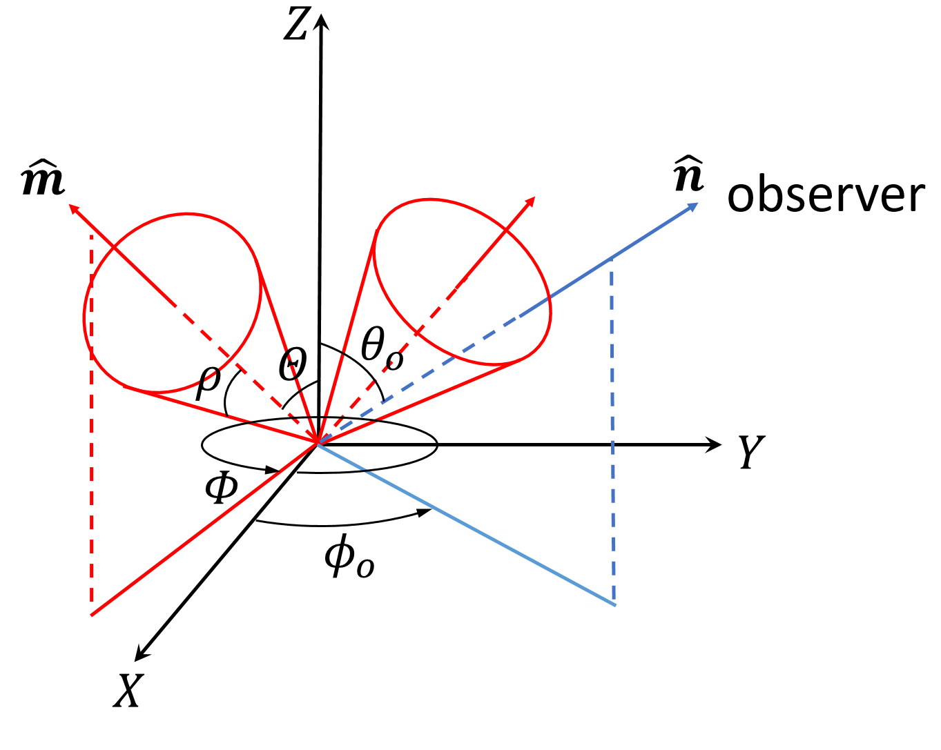
Figure 7: Cone model for pulsar radiation Gil et al. (1984); Lorimer and Kramer (2005). The unit vector along the magnetic dipole moment is denoted as $\hat{\boldsymbol{m}}$. It is the symmetric axis of the cone. The semi-open angle of the cone is denoted as $\rho$. While the star rotates, $\hat{\boldsymbol{m}}$ changes its orientation, and at some time, the cone encloses a unit vector $\hat{\boldsymbol{n}}$, so the radiation is received by the observer in the direction of $\hat{\boldsymbol{n}}$. The colatitude and the azimuth for $\hat{\boldsymbol{m}}$ and $\hat{\boldsymbol{n}}$ in the $X$-$Y$-$Z$ frame are denoted as $(\Theta,\,\Phi)$ and $(\theta_{o},\,\phi_{o})$ respectively.

A quick review of the observational signatures of free-precessing pulsars is heuristic to explore the twofold-precession case; more details can be found in e.g. Ref. Gao et al. (2020). For an axisymmetric NS, the free-precessing solution has

$$\dot{\alpha} = \frac{I^{zz}\Omega^{z}}{I^{xx}\cos\beta},$$

$$\dot{\gamma} = \Omega^{z}-\dot{\alpha}\cos\beta=-\epsilon\Omega^{z},$$ (48)

with the angle $\beta$ being constant. Therefore, the expression $\hat{\boldsymbol{m}}\cdot\hat{\boldsymbol{n}}$ as shown in Eq. (47) is simply a sum of four sinusoids of angular frequencies $\dot{\alpha}-\dot{\gamma},\,\dot{\alpha},\,\dot{\alpha}+\dot{\gamma}$, and $\dot{\gamma}$. The analysis is further simplified by the fact that the deformation $\epsilon$ is extremely small for NSs so that the frequency components $\dot{\alpha}\pm\dot{\gamma}$ are basically the same as $\dot{\alpha}$, leaving the pulsar period to be $P\approx 2\pi/\dot{\alpha}$ and modulated with a period of $P_{P}\approx 2\pi/|\dot{\gamma}|$. Here we assume that the directions of the $z$-axis and the $Z$-axis are properly chosen so that $\Omega^{z}$ and $\cos\beta$ are positive.

An exact analytical expression of the pulsar period $P$ in terms of the Euler angles was derived in Ref. Jones and Andersson (2001) by calculating the rate of the azimuthal angle of $\hat{\boldsymbol{m}}$ in the $X$-$Y$-$Z$ frame. Denote the angular coordinates of $\hat{\boldsymbol{m}}$ in the $X$-$Y$-$Z$ frame as $(\Theta,\Phi)$, then their relation with $(\chi,\delta)$ can be found by transforming the Cartesian components of $\hat{\boldsymbol{m}}$ under the rotation (8). The result is

$$\cos\Theta = \cos\beta\cos\chi+\sin\beta\sin\chi\sin{(\gamma+\delta)},$$

$$\tan\Phi = \tan{(\alpha+\Delta\Phi)},$$ (49)

where

$$\tan\Delta\Phi=\frac{\cos\beta\sin{(\gamma+\delta)}-\sin\beta\cot\chi}{\cos{(\gamma+\delta)}}.$$ (50)

The pulsar period, defined as the time intervals between $\hat{\boldsymbol{m}}$ consecutively passing through the plane formed by the $Z$-axis and the observer, is then

$$P\equiv\frac{2\pi}{\dot{\Phi}}=\frac{2\pi}{\dot{\alpha}+\Delta\dot{\Phi}}\approx\frac{2\pi}{\dot{\alpha}}\left(1-\frac{\Delta\dot{\Phi}}{\dot{\alpha}}\right),$$ (51)

where

$$\Delta\dot{\Phi}=-\dot{\gamma}\frac{\sin\beta\cot\chi\sin{(\gamma+\delta)}-\cos\beta}{\cos^{2}{(\gamma+\delta)}+\left(\sin\beta\cot\chi-\cos\beta\sin{(\gamma+\delta)}\right)^{2}}\,.$$ (52)

Equation (51) not only confirms that the pulsar period $P$ is approximately generated by the angular frequency $\dot{\alpha}$ and that the modulation on $P$ involves sinusoidal functions of $\gamma$, but also describes the time evolution of $P$ quantitatively, ready to fit observational data, say, to extract the parameters $\dot{\alpha}$, $\dot{\gamma}$, $\beta$, and $\chi$.

Besides the pulsar period, the widths of pulse signals also encode information on the motion of the star. With the cone model of the radiation beam, it is defined as the change of the azimuthal angle of $\hat{\boldsymbol{m}}$ in the $X$-$Y$-$Z$ frame during the time when $\hat{\boldsymbol{n}}$ is inside the cone, namely

$$W\equiv\Phi_{2}-\Phi_{1},$$ (53)

where $\Phi_{1}$ and $\Phi_{2}$ are the azimuthal angle $\Phi$ solved from the equation of the inequality (44) with

$$\hat{\boldsymbol{m}}\cdot\hat{\boldsymbol{n}}=\sin\Theta\sin\theta_{0}\cos{(\Phi-\phi_{o})}+\cos\Theta\cos\theta_{o}.$$ (54)

Fortunately, because $|\dot{\gamma}|$ is much smaller than $\dot{\Phi}\approx\dot{\alpha}$, the angle $\Theta$, given by the first equation in Eqs. (49), can be treated as unchanged during $\Phi$ changing from $\Phi_{1}$ to $\Phi_{2}$ so that the roots $\Phi_{1}$ and $\Phi_{2}$ are symmetric about the azimuthal angle $\phi_{o}$ of the observer, namely,

$$\Phi_{1}\approx\phi_{o}-\frac{W}{2},\quad\Phi_{2}\approx\phi_{o}+\frac{W}{2},$$ (55)

and hence, as given in Refs. Gil et al. (1984); Lorimer and Kramer (2005), setting the expression (54) equal to $\cos\rho$ leads to an analytical expression for $W$,

$$\cos{\frac{W}{2}}\approx\frac{\cos\rho-\cos\Theta\cos\theta_{o}}{\sin\Theta\sin\theta_{o}}.$$ (56)

When the time dependence of $\Theta$ is put back in Eq. (56), it describes the modulated pulse width at the period $P_{P}\approx 2\pi/|\dot{\gamma}|$. By fitting this equation to observational data, the parameters $\dot{\gamma},\,\rho$, and $\theta_{o}$ can be extracted.

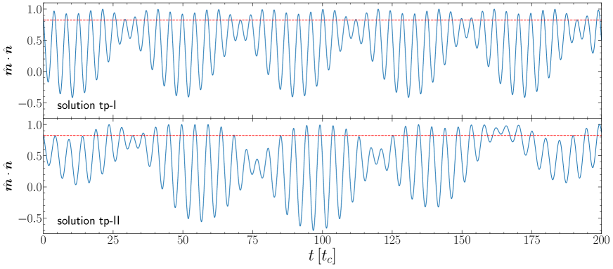
Figure 8: Time evolutions of $\hat{\boldsymbol{m}}\cdot\hat{\boldsymbol{n}}$ using the numerical solutions in Figs. 2 and 3. The constant angles $\theta_{o}$ and $\chi$ are taken to be $0.8\,{\rm rad}$ and $0.5\,{\rm rad}$ in the plots. The red dashed lines represent the cosine value of $\rho=0.6\,{\rm rad}$, illustrating the time segments when $\hat{\boldsymbol{m}}\cdot\hat{\boldsymbol{n}}$ is above $\cos\rho$ so that the signal is observed under the corresponding setup. With our choice of $\epsilon_{r}=0.1$ in the numerical solutions, the time unit is $t_{c}\sim 10^{-3}\,$s if the density of the NS is $\rho_{\rm NS}\sim 10^{15}\,{\rm g}/{\rm cm}^{3}$.

Let us now turn to the Lorentz-violating twofold-precession case. Similar characteristics of pulse signals exist. In fact, Eqs. (51) and (56) apply straightforwardly as long as $|\dot{\gamma}|\ll\dot{\alpha}$. This is exactly the regime where the perturbation solution of the twofold precession works. Neglecting the oscillating terms, $\alpha^{(1)}$ and $\beta^{(1)}$, the perturbation solution has

$$\dot{\alpha} \approx a=\frac{I^{zz}\Omega^{z}}{I^{xx}\cos\beta_{0}}-a^{(1)},$$

$$\dot{\gamma} = \Omega^{z}-\dot{\alpha}\cos\beta\approx-\epsilon\Omega^{z}+\cos\beta_{0}\,a^{(1)},$$ (57)

where the free-precessing angular frequencies, $\dot{\alpha}$ and $\dot{\gamma}$, are shifted due to Lorentz violation. By fitting Eqs. (51) and (56) to observational data, we will be able to extract the two shifted frequencies, $\dot{\alpha}$ and $\dot{\gamma}$, and the angular parameters $\beta_{0}$, $\chi$, $\rho$, and $\theta_{o}$.

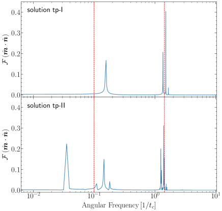
Figure 9: Fourier transformations for $\hat{\boldsymbol{m}}\cdot\hat{\boldsymbol{n}}$ in Fig. 8. The dashed red vertical lines mark $\dot{\alpha}\approx 1.438$ and $|\dot{\gamma}|=0.1$, which are the values from the free-precessing equations (48) with $I^{zz}/I^{xx}=1.1$, $\Omega^{z}=1$, and $\beta=0.7$. As we have taken $\epsilon_{r}=0.1$, the frequency unit is $1/t_{c}\sim 1000\,{\rm rad/s}$ if the density of the NS is $\rho_{\rm NS}\sim 10^{15}\,{\rm g}/{\rm cm}^{3}$.

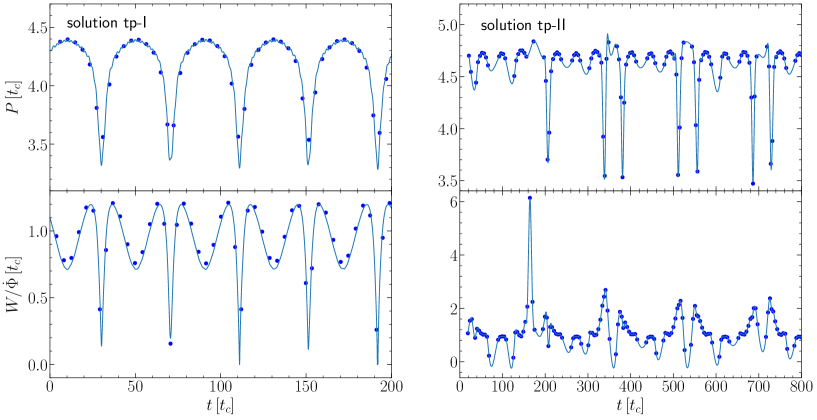
Figure 10: Discrete time series of pulsar period and time segment associated to pulse width, solved from $\hat{\boldsymbol{m}}\cdot\hat{\boldsymbol{n}}=\cos\rho$ with $\hat{\boldsymbol{m}}\cdot\hat{\boldsymbol{n}}$ from Fig. 8 and $\rho=0.6\,{\rm rad}$. The left plots are for the solution tp-I where the lines are generated by Eqs. (51) and (56). The right plots are for the solution tp-II where Eqs. (51) and (56) fail to approximate the discrete points and the lines are spline interpolations of the discrete points.

A crucial defect here is that once $\dot{\alpha}$ and $\dot{\gamma}$ are extracted, we are unable to deduce $\Omega^{z}$, $\epsilon$, and $a^{(1)}$ simultaneously. One more piece of information on the three quantities is required from the observational data. It involves details of the pattern of $\hat{\boldsymbol{m}}\cdot\hat{\boldsymbol{n}}$ that are beyond the perturbation approximation of $\dot{\alpha}$ and $\dot{\gamma}$ in Eqs. (57), and inevitably invokes numerical solutions of the twofold-precession motion. Numerical calculations for $\hat{\boldsymbol{m}}\cdot\hat{\boldsymbol{n}}$ are also necessary for another important reason. When $\dot{\gamma}$ is not much smaller than $\dot{\alpha}$, the perturbation solution breaks down, and to make matters worse, Eqs. (51) and (56) are also not valid any more, so there are no analytical templates to fit the pulsar period and the pulse width. In this case, the inequality (44) needs to be solved numerically to deduce discrete time series of pulsar period and pulse width to fit observational data. The rotation of the star, the parameters $\epsilon$, $\chi$, $\rho$, and $\theta_{o}$, and the coefficients for Lorentz violation $\bar{s}^{XX}$, $\bar{s}^{YY}$, and $\bar{s}^{ZZ}$, might be determined via elaborate numerical calculations and careful treatments. Of course, other measurements, like the polarization properties of the radiation, might provide extra information and can be combined to derive a full solution. This lays beyond the scope of the current work.

In Fig. 8, the time evolutions of $\hat{\boldsymbol{m}}\cdot\hat{\boldsymbol{n}}$ using the two numerical solutions in Fig. 2 (solution tp-I) and Fig. 3 (solution tp-II) are displayed, while Fig. 9 depicts the corresponding angular frequency spectra. A decisive characteristic shows up in the case of the solution that invalidates the perturbation approach (namely, solution tp-II). That is the extra smallest frequency component appearing in the lower plot of Fig. 9. This frequency corresponds to the average angular velocity at which the angular momentum of the star precesses about the $Z$-axis. Though no simple approximate expression relates it to the coefficients for Lorentz violation, numerical calculations indicate that this angular frequency has the same order of magnitude as the coefficients for Lorentz violation under the dimensionless parametrization using the time unit defined in Eq. (35), which for realistic NSs has an estimation

$$t_{c}\approx\sqrt{\frac{15}{4\pi}\frac{1}{\rho_{\rm NS}\epsilon_{r}}}\sim 1{\rm s},$$ (58)

with density $\rho_{\rm NS}\sim 10^{15}\,{\rm g}/{\rm cm}^{3}$ and rigid deformation $\epsilon_{r}\sim 10^{-8}$ assumed. The extra frequency component does not show up in the case of solution tp-I. Because in that case, the angular momentum of the star is almost aligned with the $Z$-axis, so the precession of the angular momentum around the $Z$-axis caused by Lorentz violation degenerates with the free precession, generating a total precession rate $\dot{\alpha}$ approximately given by the first equation in Eqs. (57) where the Lorentz-violating contribution $a^{(1)}$ is unable to be decoupled.

In Fig. 10, discrete time series of pulsar period and of time segment corresponding to pulse width calculated by solving the inequality (44) using the numerical templates of $\hat{\boldsymbol{m}}\cdot\hat{\boldsymbol{n}}$ from Fig. 8 are plotted. For the case of the solution tp-I (left panels of Fig. 10), the smooth curves that approximate the discrete points are generated using Eqs. (51) and (56). They fit very well. For the case of the solution tp-II (right panels of Fig. 10), Eqs. (51) and (56) fail to approximate the discrete series, so we have to interpolate the points to reveal the trends of them. Note that in both cases there is a period about $40\,t_{c}$ originated from the angular frequency between $0.1\,t_{c}^{-1}$ and $0.2\,t_{c}^{-1}$ in Fig. 9, while in the right panels a period about $180\,t_{c}$ shows up—more perceivable in the pulsar-period plot than in the pulse-width plot—reflecting the characteristic angular frequency between $0.03\,t_{c}^{-1}$ and $0.04\,t_{c}^{-1}$ in the lower panel of Fig. 9.

III.3 Twofold-precession motion and continuous GWs

The quadrupole GW radiated by a freely precessing rigid body was calculated in Refs. Zimmermann and Szedenits (1979); Zimmermann (1980). To investigate the quadrupole radiation by a rigid body undergoing the twofold-precession motion due to Lorentz violation, we generalize Zimmermann’s calculation Zimmermann (1980) to any rotating rigid body with torques.

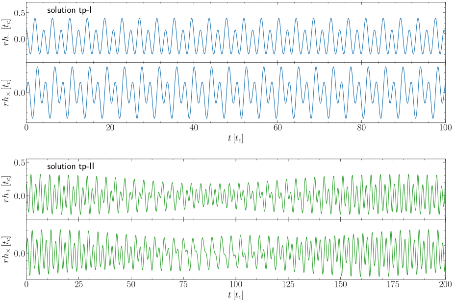
Figure 11: Continuous GWs from NSs subjected to the solutions tp-I and tp-II. The angular coordinates of the observer are taken to be $\theta_{o}=0.8\,{\rm rad}$ and $\phi_{o}=0$ in the plots. Time and distance are parametrized using the time unit $t_{c}$ defined in Eq. (35), which is at the order of $10^{-3}\,$s with our choice of $\epsilon_{r}=0.1$ in the numerical solutions and $\rho_{\rm NS}\sim 10^{15}\,{\rm g}/{\rm cm}^{3}$ assumed for the density of the NS.

The metric perturbation in the $X$-$Y$-$Z$ frame is given by the quadrupole formula

$$h^{IJ}=-\frac{2}{r}\ddot{I}^{IJ},$$ (59)

where $r$ is the distance from the star to the observer, and the double dots denote the second time derivative. The time dependence of the inertial-frame components of the moment of inertia tensor originates in the rotation matrix via

$$I^{IJ}=R^{iI}R^{jJ}I^{ij},$$ (60)

while the body-frame components of the moment of inertia tensor are constant. The derivatives of $R^{iI}$ can be derived by noticing that the body-frame axes undergo an infinitesimal rotation

$$\hat{\boldsymbol{e}}_{i}\rightarrow\hat{\boldsymbol{e}}_{i}+dt\,\boldsymbol{\Omega}\times\hat{\boldsymbol{e}}_{i},$$ (61)

at the instant when the body rotates with an angular velocity $\boldsymbol{\Omega}$. The change of $R^{iI}$ is therefore $dt\,\left(\boldsymbol{\Omega}\times\hat{\boldsymbol{e}}_{i}\right)\cdot\hat{\boldsymbol{e}}_{I}$, giving

$$\frac{dR^{iI}}{dt}=\left(\boldsymbol{\Omega}\times\hat{\boldsymbol{e}}_{i}\right)\cdot\hat{\boldsymbol{e}}_{I}=\epsilon^{IJK}\Omega^{J}R^{iK},$$ (62)

where $\epsilon^{IJK}$ is the Levi-Civita symbol. Equation (62) can be used to calculate $\dot{I}^{IJ}$. When combined with the equation of motion

$$\dot{I}^{IJ}\Omega^{J}+I^{IJ}\dot{\Omega}^{J}=\Gamma^{I},$$ (63)

$\boldsymbol{\dot{\Omega}}$ can be solved in terms of $\boldsymbol{\Omega}$ and the torque $\boldsymbol{\Gamma}$. Then, the demanded second derivative $\ddot{I}^{IJ}$ can be found to take the form

$$\ddot{I}^{IJ}=R^{iI}R^{jJ}A^{ij},$$ (64)

with the help of the derivative of Eq. (62). The body-frame tensor $A^{ij}$ is lengthy in general, but much simplified when the body frame diagonalizes the moment of inertia tensor, which is the case in our setup. The components then read

$$A^{xx} = 2\left(\Delta_{2}\left(\Omega^{y}\right)^{2}-\Delta_{3}\left(\Omega^{z}\right)^{2}\right),$$

$$A^{yy} = 2\left(\Delta_{3}\left(\Omega^{z}\right)^{2}-\Delta_{1}\left(\Omega^{x}\right)^{2}\right),$$

$$A^{zz} = 2\left(\Delta_{1}\left(\Omega^{x}\right)^{2}-\Delta_{2}\left(\Omega^{y}\right)^{2}\right),$$

$$A^{xy} = \left(\frac{\left(\Delta_{3}\right)^{2}}{I^{zz}}+\Delta_{1}-\Delta_{2}\right)\Omega^{x}\Omega^{y}+\frac{\Delta_{3}}{I^{zz}}\Gamma^{z},$$

$$A^{xz} = \left(\frac{\left(\Delta_{2}\right)^{2}}{I^{yy}}+\Delta_{3}-\Delta_{1}\right)\Omega^{x}\Omega^{z}+\frac{\Delta_{2}}{I^{yy}}\Gamma^{y},$$

$$A^{yz} = \left(\frac{\left(\Delta_{1}\right)^{2}}{I^{xx}}+\Delta_{2}-\Delta_{3}\right)\Omega^{y}\Omega^{z}+\frac{\Delta_{1}}{I^{xx}}\Gamma^{x},$$ (65)

where $(\Omega^{x},\,\Omega^{y},\,\Omega^{z})$ are the body-frame velocity components given in terms of the Euler angles and their derivatives in Eqs. (22), and the body-frame torque components $(\Gamma^{x},\,\Gamma^{y},\,\Gamma^{z})$ can be calculated from the anisotropic potential $\delta U$ via

$$\Gamma^{x} = -\frac{\sin\gamma}{\sin\beta}\,\partial_{\alpha}\delta U-\cos\gamma\,\partial_{\beta}\delta U+\cot\beta\sin\gamma\,\partial_{\gamma}\delta U,$$

$$\Gamma^{y} = -\frac{\cos\gamma}{\sin\beta}\,\partial_{\alpha}\delta U+\sin\gamma\,\partial_{\beta}\delta U+\cot\beta\cos\gamma\,\partial_{\gamma}\delta U,$$

$$\Gamma^{z} = -\partial_{\gamma}\delta U.$$ (66)

The symbols $\Delta_{1},\,\Delta_{2}$, and $\Delta_{3}$ follow the definition of Zimmermann (1980),

$$\Delta_{1}=I^{yy}-I^{zz},\quad\Delta_{2}=I^{zz}-I^{xx},\quad\Delta_{3}=I^{xx}-I^{yy}.$$ (67)

It is plain that Eqs. (65) go back to the result of Zimmermann (1980) when $\boldsymbol{\Gamma}=0$.

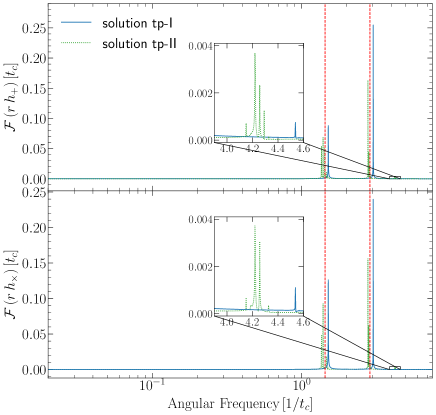
Figure 12: Fourier transformations for the continuous GWs shown in Fig. 11. The dashed red vertical lines mark $\dot{\alpha}\approx 1.438$ and $2\dot{\alpha}\approx 2.876$, which are the angular frequencies of the continuous GWs from a free-precessing NS with $I^{zz}/I^{xx}=1.1,\,\Omega^{z}=1$, and $\beta=0.7$. As we have taken $\epsilon_{r}=0.1$, the frequency unit is $1/t_{c}\sim 1000\,{\rm rad/s}$ if the density of the NS is $\rho_{\rm NS}\sim 10^{15}\,{\rm g}/{\rm cm}^{3}$.

As we restrict ourselves to spheroids, the tensor $A^{ij}$ is further simplified by $I^{xx}=I^{yy}$ and $\Gamma^{z}=0$. In the absence of Lorentz violation, the star precesses freely, and the tensor $\ddot{I}^{IJ}$ has a simple form,

$$\ddot{I}^{IJ} = \frac{1}{2}\Delta_{2}\,\dot{\alpha}^{2}\sin{2\beta}$$ (68)

$$\times\begin{pmatrix}2\cos{2\alpha}\tan\beta&2\sin{2\alpha}\tan\beta&-\sin\alpha\\ 2\sin{2\alpha}\tan\beta&-2\cos{2\alpha}\tan\beta&\cos\alpha\\ -\sin\alpha&\cos\alpha&0\end{pmatrix},$$

which tells that $h^{IJ}$ is a spherical wave with exactly two frequency components, namely $\dot{\alpha}$ and $2\dot{\alpha}$. When Lorentz violation presents and the star is subjected to the twofold-precession motion, the tensor $\ddot{I}^{IJ}$ becomes complicated as $\dot{\beta}$ no longer vanishes. But if we only consider motions given by the perturbation solution, we expect Eq. (68) to be a fair approximation and that the continuous GW still has two frequency components, $\dot{\alpha}$ and $2\dot{\alpha}$, with $\dot{\alpha}$ being the Lorentz-violating shifted angular frequency given by the first equation in Eqs. (57).

For an observer with colatitude $\theta_{o}$ and azimuth $\phi_{o}$ in the $X$-$Y$-$Z$ frame, the basis to decompose the two physical degrees of freedom for the continuous GW can be taken as

$$\boldsymbol{e}_{+}\equiv\hat{\boldsymbol{\theta}}_{o}\otimes\hat{\boldsymbol{\theta}}_{o}-\hat{\boldsymbol{\phi}}_{o}\otimes\hat{\boldsymbol{\phi}}_{o},\quad\boldsymbol{e}_{\times}\equiv\hat{\boldsymbol{\theta}}_{o}\otimes\hat{\boldsymbol{\phi}}_{o}+\hat{\boldsymbol{\phi}}_{o}\otimes\hat{\boldsymbol{\theta}}_{o},$$ (69)

where

$$\hat{\boldsymbol{\theta}}_{o} = \cos\theta_{o}\cos\phi_{o}\,\hat{\boldsymbol{e}}_{X}+\cos\theta_{o}\sin\phi_{o}\,\hat{\boldsymbol{e}}_{Y}-\sin\theta_{o}\hat{\boldsymbol{e}}_{Z},$$

$$\hat{\boldsymbol{\phi}}_{o} = -\sin\phi_{o}\,\hat{\boldsymbol{e}}_{X}+\cos\phi_{o}\,\hat{\boldsymbol{e}}_{Y}.$$ (70)

Then the “+” and the “$\times$” components of the continuous GW are

$$h_{+} = \frac{1}{2}\left(\hat{\theta}_{o}^{I}\,\hat{\theta}_{o}^{J}-\hat{\phi}_{o}^{I}\,\hat{\phi}_{o}^{J}\right)h^{IJ}=-\frac{1}{r}\left(\hat{\theta}_{o}^{I}\,\hat{\theta}_{o}^{J}-\hat{\phi}_{o}^{I}\,\hat{\phi}_{o}^{J}\right)\ddot{I}^{IJ},$$

$$h_{\times} = \frac{1}{2}\left(\hat{\theta}_{o}^{I}\,\hat{\phi}_{o}^{J}+\hat{\phi}_{o}^{I}\,\hat{\theta}_{o}^{J}\right)h^{IJ}=-\frac{1}{r}\left(\hat{\theta}_{o}^{I}\,\hat{\phi}_{o}^{J}+\hat{\phi}_{o}^{I}\,\hat{\theta}_{o}^{J}\right)\ddot{I}^{IJ},$$ (71)

where $\hat{\theta}_{o}^{I}$ and $\hat{\phi}_{o}^{I}$ are the components of $\hat{\boldsymbol{\theta}}_{o}$ and $\hat{\boldsymbol{\phi}}_{o}$ in the $X$-$Y$-$Z$ frame as shown in Eqs. (70).

When continuous GWs from NSs are detected, Eqs. (71) can be used as template waveforms to match observational data. Similar to the analysis of pulsar signal, to extract the coefficients for Lorentz violation, $\bar{s}^{XX}$, $\bar{s}^{YY}$, $\bar{s}^{ZZ}$, and the NS parameters, $\epsilon$, $\Omega^{z}$, $\theta_{o}$, $r$, from observational data, elaborate numerical calculations are required. Using the two numerical solutions in Figs. 2 and 3 to calculate $\ddot{I}^{IJ}$, we plot the corresponding waveforms in Fig. 11 and their Fourier transformations in Fig. 12. Tiny high frequency components in the spectra are found. They are featured in the subplots of Fig. 12 and turn out to be exactly three times of the fundamental frequencies, which are represented by the peaks near $1.438\,t_{c}^{-1}$ and can be regarded as the average values of $\dot{\alpha}$ for the twofold-precession motions. Frequencies higher than the third harmonic exist, but their amplitudes are even much smaller. We point out that unlike the pulsar signal of solution tp-II, there is no low frequency at the order of the coefficients for Lorentz violation in the continuous GW spectra. However, the advantage of continuous GW signal is that both solution tp-I and solution tp-II exhibit the third harmonic, characterizing the deviation of the waveform from that of a free-precessing NS, though in the case of solution tp-I, the amplitude of the third harmonic is further suppressed. These Lorentz-violating features are worth looking for and may reveal new physics beyond the current understanding.

IV conclusion

Lorentz violation modifies the Newtonian potential by an anisotropic correction, generating a torque on spheroidal stars that forces the otherwise conserved angular momentum of the star to precess around a preferred direction defined by the coefficients for Lorentz violation. To solve the motion rigorously, we first calculate the anisotropic gravitational self-energy of the star caused by Lorentz violation in the minimal gravitational SME in Sec. II.1. The result is proved to be equivalent to that of Nordtvedt (1987) when the star is treated as a stationary spinning fluid star in equilibrium so the tensor virial relation holds. Discrepancy occurs when the star possesses a rigid deformation which invalidates the tensor virial relation. Besides stationary spin, free precession is also a solution of motion for such stars in the absence of torques.

Then in Sec. II.2, the forced precession caused by the Lorentz-violating torque on stationary spinning stars and on free-precessing stars is explicitly calculated using perturbation method to solve the rotational equations of motion. Interestingly, we find that the direction of the forced precession on stationary spinning stars is opposite to the direction of the forced precession on free-precessing stars as shown in Eq. (32). Numerical solutions are explored to check the validity of the perturbation approach. Initial values for which the perturbation approach fails are identified. The study of the solutions is finished by clarifying that the preferred directions around which the forced precession happens are exactly the eigenvectors of the matrix $\bar{s}^{ij}$. An interesting result is that when the matrix $\bar{s}^{ij}$ acquires 3 different eigenvalues, the forced precession is unstable if it is around the eigenvector corresponding to the middle eigenvalue. This is similar to the well-known Dzhanibekov effect (or the tennis racket theorem).

After the solutions of motion are studied thoroughly, we apply them to explore observational consequences for NSs in Sec. III. Section III.1 treats the two solitary pulsars in Ref. Shao et al. (2013) as stationary spinning spheroids at zeroth order, and sets bounds on the coefficients for Lorentz violation by attributing any possible tiny alteration of the NSs’ orientations hidden in observational uncertainties to the forced precession due to Lorentz violation. With the connection between the SME coefficients $\bar{s}^{ij}$ and the PPN coefficient $\alpha_{2}$ shown in Eq. (5), the constraints obtained here are consistent with the ones for the $\alpha_{2}$ coefficient in Ref. Shao et al. (2013). However, our “maximal-reach” constraints obtained from the two solitary pulsars are 3 to 5 orders of magnitude better than those in Ref. Shao (2014). The exactly same two solitary pulsars are used there but together with another 11 binary pulsars for a global analysis. Notice that here we are using a different coordinate frame from that of Ref. Shao (2014) so a plain comparison is only heuristic. Nevertheless, this suggests that the orbital motions of the binary pulsars are less sensitive to Lorentz violation than the rotational motions of the solitary pulsars. Therefore, we urge observers to analyze the stability of pulsar spins—possibly via the pulse profile stability as it was done by Shao et al. (2013)—with more suitable systems, and put tighter bounds on the coefficients for Lorentz violation.

In Sec. III.2 and Sec. III.3, pulsar signals and continuous GWs from Lorentz-violating-affected free-precessing NSs are investigated. When the angular momentum of the star is close to the preferred direction around which the forced precession happens, the spectra of the signals are very much like those from a free-precessing NS. The forced precession does shift frequencies in the spectra, but the contribution from it is practically unable to be decoupled from the free-precessing frequency components. When the angular momentum of the star makes a relatively large angle to the preferred direction around which the forced precession happens, decisive characteristics that are worth searching for show up in the spectra. For pulsar signals, the signature is an extremely low frequency component as shown in the lower plot of Fig. 9. The observables, namely the pulsar period and the pulse width, are not only modulated by the average rate of the Euler angle $\gamma$, but also modulated by this frequency (right plots in Fig. 10). The polarization characteristics of pulsar pulses are interesting to investigate in future studies, and they could provide more information on the rotation of the NS and its radiation properties. For GWs, the signature is the third harmonic shown in the subplots of Fig. 12. Free-precessing spheroidal NSs emit continuous GWs only at the first and the second harmonics of the rate of the Euler angle $\alpha$. But once affected by Lorentz violation, the continuous GW emitted by the star is no longer a simple sum of sinusoidal functions. The waveform generally involves all harmonics of the average rate of the Euler angle $\alpha$, with the amplitudes decrease rapidly after the first two of them.

The characteristic frequencies in the spectra of the signals are qualitative supports for Lorentz violation if observed. To extract quantitative values of the coefficients for Lorentz violation, as well as the physical parameters of the NS, numerical calculations are necessary to fit observational data. Tentative candidates of free-precessing NSs are proposed in pulsar observations Stairs et al. (2000); Shabanova et al. (2001), while searches of continuous GWs have not yet confidently identified any positive detections Abbott et al. (2019); Covas and Sintes (2020); Dergachev and Papa (2020); Papa et al. (2020); Steltner et al. (2020); Zhang et al. (2021). Our study supplies necessary templates for potential new tests of Lorentz violation that take advantage of the two state-of-the-art observation channels in the era of multimessenger astronomy. Once free-precessing NSs are unambiguously identified, the new tests using their modulated pulsar signals and continuous GWs are bound to enrich our fundamental knowledge on Lorentz symmetry of our spacetime.

Appendix A The constant $C$ for uniform spheroids

Using the results on Maclaurin spheroids summarized in Refs. Chandrasekhar and Lebovitz (1962); Poisson and Will (2014), we can explicitly write down the constant $C$ in terms of the eccentricity defined as

$$e\equiv\sqrt{1-\left(\frac{a_{3}}{a_{1}}\right)^{2}},$$ (72)

for a spheroid (10) with uniform density. We start with the Newtonian potential (16) inside an ellipsoid of uniform density,

$$\Phi=-\pi\rho\left(A_{0}-A_{1}x^{2}-A_{2}y^{2}-A_{3}z^{2}\right).$$ (73)

The constants $A_{0}$, $A_{1}$, $A_{2}$, and $A_{3}$ happen to have closed-form results for spheroids,

$$A_{0} = 2a_{1}^{2}\sqrt{1-e^{2}}\frac{\arcsin{e}}{e}=2a_{1}^{2}\left(1-\frac{1}{3}e^{2}+O(e^{4})\right),$$

$$A_{1} = A_{2}=\frac{\sqrt{1-e^{2}}}{e^{2}}\left(\frac{\arcsin{e}}{e}-\sqrt{1-e^{2}}\right)$$

$$\quad\ =\frac{2}{3}\left(1-\frac{1}{5}e^{2}+O(e^{2})\right),$$

$$A_{3} = \frac{2}{e^{2}}\left(1-\sqrt{1-e^{2}}\frac{\arcsin{e}}{e}\right)=\frac{2}{3}\left(1+\frac{2}{5}e^{2}+O(e^{2})\right).$$ (74)

It then follows that the constant $C$ is

$$C = \frac{1}{2}\left(U^{xx}-U^{zz}\right)=\frac{4\pi^{2}}{15}\rho^{2}a_{1}^{2}a_{3}\left(a_{1}^{2}A_{1}-a_{3}^{2}A_{3}\right)$$ (75)

$$= \frac{16\pi^{2}}{225}\rho^{2}a_{1}^{4}a_{3}\left(e^{2}+O(e^{4})\right).$$

We point out that the equilibrium condition

$$\frac{p}{\rho}=-\Phi+\frac{1}{2}{|\boldsymbol{\Omega}}|^{2}\left(x^{2}+y^{2}\right)+{\rm const.}\,,$$ (76)

on the surface where $p=0$ implies

$$|{\boldsymbol{\Omega}}|^{2}=2\pi\rho\left(A_{1}-\frac{a_{3}^{2}}{a_{1}^{2}}A_{3}\right).$$ (77)

As the angular velocity ${\boldsymbol{\Omega}}$ is along the $z$-axis, we directly see

$$T_{\rm rot}=\frac{1}{2}I^{zz}|{\boldsymbol{\Omega}}|^{2}=2C,$$ (78)

where $I^{zz}=8\pi/15\,\rho a_{1}^{4}a_{3}$ has been used. It is also worth pointing out that both the eccentricity defined in Eq. (72) and the oblateness defined in Eq. (19) characterize the deviation of a spheroid from a sphere. For a uniform spheroid, they are simply related via

$$\epsilon=\frac{e^{2}}{2-e^{2}}.$$ (79)

References

- Kostelecký and Samuel (1989a) V. A. Kostelecký and S. Samuel, Phys. Rev. D 39, 683 (1989a).
- Kostelecký and Samuel (1989b) V. A. Kostelecký and S. Samuel, Phys. Rev. Lett. 63, 224 (1989b).
- Kostelecký and Potting (1991) V. A. Kostelecký and R. Potting, Nucl. Phys. B 359, 545 (1991).
- Will and Nordtvedt (1972) C. M. Will and K. Nordtvedt, Jr., Astrophys. J. 177, 757 (1972).
- Will (2018) C. M. Will, Theory and Experiment in Gravitational Physics (Cambridge University Press, 2018).
- Kostelecký and Russell (2011) V. A. Kostelecký and N. Russell, Rev. Mod. Phys. 83, 11 (2011), arXiv:0801.0287 [hep-ph] .
- Shao and Wex (2016) L. Shao and N. Wex, Sci. China Phys. Mech. Astron. 59, 699501 (2016), arXiv:1604.03662 [gr-qc] .
- Colladay and Kostelecký (1997) D. Colladay and V. A. Kostelecký, Phys. Rev. D 55, 6760 (1997), arXiv:hep-ph/9703464 .
- Colladay and Kostelecký (1998) D. Colladay and V. A. Kostelecký, Phys. Rev. D 58, 116002 (1998), arXiv:hep-ph/9809521 .
- Kostelecký (2004) V. A. Kostelecký, Phys. Rev. D 69, 105009 (2004), arXiv:hep-th/0312310 .
- Bailey and Kostelecký (2006) Q. G. Bailey and V. A. Kostelecký, Phys. Rev. D 74, 045001 (2006), arXiv:gr-qc/0603030 .
- Bluhm and Kostelecký (2005) R. Bluhm and V. A. Kostelecký, Phys. Rev. D 71, 065008 (2005), arXiv:hep-th/0412320 .
- Bailey et al. (2015) Q. G. Bailey, V. A. Kostelecký, and R. Xu, Phys. Rev. D 91, 022006 (2015), arXiv:1410.6162 [gr-qc] .
- Shao (2014) L. Shao, Phys. Rev. Lett. 112, 111103 (2014), arXiv:1402.6452 [gr-qc] .
- Gao et al. (2020) Y. Gao, L. Shao, R. Xu, L. Sun, C. Liu, and R.-X. Xu, Mon. Not. Roy. Astron. Soc. 498, 1826 (2020), arXiv:2007.02528 [astro-ph.HE] .
- Will (2014) C. M. Will, Living Rev. Rel. 17, 4 (2014), arXiv:1403.7377 [gr-qc] .
- Nordtvedt (1987) K. Nordtvedt, Astrophys. J. 320, 871 (1987).
- Landau and Lifshitz (1960) L. D. Landau and E. M. Lifshitz, Mechanics (Oxford, 1960).
- Xu et al. (2021) R. Xu, Y. Gao, and L. Shao, Galaxies 9, 12 (2021), arXiv:2101.09431 [gr-qc] .
- Poisson and Will (2014) E. Poisson and C. M. Will, Gravity: Newtonian, Post-Newtonian, Relativistic (Cambridge University Press, Cambridge, England, 2014).
- Chandrasekhar and Lebovitz (1962) S. Chandrasekhar and N. R. Lebovitz, Astrophys. J. 136, 1037 (1962).
- Jones and Andersson (2001) D. I. Jones and N. Andersson, Mon. Not. R. Astron. Soc. 324, 811 (2001), arXiv:astro-ph/0011063 [astro-ph] .
- Zimmermann and Szedenits (1979) M. Zimmermann and E. Szedenits, Phys. Rev. D 20, 351 (1979).
- Gao and Shao (2020) Y. Gao and L. Shao, (2020), arXiv:2011.04472 [astro-ph.HE] .
- Altschul (2007) B. Altschul, Phys. Rev. D 75, 023001 (2007), arXiv:hep-ph/0608094 .
- Xu et al. (2020) R. Xu, J. Zhao, and L. Shao, Phys. Lett. B 803, 135283 (2020), arXiv:1909.10372 [gr-qc] .
- Kostelecký and Mewes (2002) V. A. Kostelecký and M. Mewes, Phys. Rev. D 66, 056005 (2002), arXiv:hep-ph/0205211 .
- Poinsot (1851) L. Poinsot, Theórie nouvelle de la rotation des corps (Bachelier, Paris, France, 1851).
- Shao et al. (2013) L. Shao, R. N. Caballero, M. Kramer, N. Wex, D. J. Champion, and A. Jessner, Class. Quant. Grav. 30, 165019 (2013), arXiv:1307.2552 [gr-qc] .
- Shao (2020) L. Shao, in 8th Meeting on CPT and Lorentz Symmetry (2020) pp. 170–173, arXiv:1905.08405 [gr-qc] .
- Stairs et al. (2000) I. Stairs, A. Lyne, and S. Shemar, Nature 406, 484 (2000).
- Lorimer and Kramer (2005) D. R. Lorimer and M. Kramer, Handbook of Pulsar Astronomy (Cambridge University Press, Cambridge, England, 2005).
- Tasson (2020) J. D. Tasson, in 8th Meeting on CPT and Lorentz Symmetry (2020) pp. 13–16, arXiv:1907.08106 [hep-ph] .
- Gil et al. (1984) J. Gil, P. Gronkowski, and W. Rudnicki, A&A 132, 312 (1984).
- Zimmermann (1980) M. Zimmermann, Phys. Rev. D 21, 891 (1980).
- Shabanova et al. (2001) T. Shabanova, A. Lyne, and J. Urama, Astrophys. J. 552, 321 (2001), arXiv:astro-ph/0101282 .
- Abbott et al. (2019) B. Abbott et al. (LIGO Scientific, Virgo), Phys. Rev. D 100, 024004 (2019), arXiv:1903.01901 [astro-ph.HE] .
- Covas and Sintes (2020) P. B. Covas and A. M. Sintes, Phys. Rev. Lett. 124, 191102 (2020), arXiv:2001.08411 [gr-qc] .
- Dergachev and Papa (2020) V. Dergachev and M. A. Papa, Phys. Rev. Lett. 125, 171101 (2020), arXiv:2004.08334 [gr-qc] .
- Papa et al. (2020) M. A. Papa, J. Ming, E. V. Gotthelf, B. Allen, R. Prix, V. Dergachev, H.-B. Eggenstein, A. Singh, and S. J. Zhu, Astrophys. J. 897, 22 (2020), arXiv:2005.06544 [astro-ph.HE] .
- Steltner et al. (2020) B. Steltner, M. Papa, H.-B. Eggenstein, B. Allen, V. Dergachev, R. Prix, B. Machenschalk, S. Walsh, S. Zhu, and S. Kwang, (2020), arXiv:2009.12260 [astro-ph.HE] .
- Zhang et al. (2021) Y. Zhang, M. A. Papa, B. Krishnan, and A. L. Watts, Astrophys. J. Lett. 906, L14 (2021), arXiv:2011.04414 [astro-ph.HE] .