Improved Contrastive Divergence Training of Energy-Based Model

Abstract

Contrastive divergence is a popular method of training energy-based models, but is known to have difficulties with training stability. We propose an adaptation to improve contrastive divergence training by scrutinizing a gradient term that is difficult to calculate and is often left out for convenience. We show that this gradient term is numerically significant and in practice is important to avoid training instabilities, while being tractable to estimate. We further highlight how data augmentation and multi-scale processing can be used to improve model robustness and generation quality. Finally, we empirically evaluate stability of model architectures and show improved performance on a host of benchmarks and use cases,such as image generation, OOD detection, and compositional generation.

1 Introduction

Energy-Based models (EBMs) have received an influx of interest recently and have been applied to realistic image generation (Han et al., 2019; Du & Mordatch, 2019), 3D shapes synthesis (Xie et al., 2018b) , out of distribution and adversarial robustness (Lee et al., 2018; Du & Mordatch, 2019; Grathwohl et al., 2019), compositional generation (Hinton, 1999; Du et al., 2020a), memory modeling (Bartunov et al., 2019), text generation (Deng et al., 2020), video generation (Xie et al., 2017), reinforcement learning (Haarnoja et al., 2017; Du et al., 2019), continual learning (Li et al., 2020), protein design and folding (Ingraham et al., ; Du et al., 2020b) and biologically-plausible training (Scellier & Bengio, 2017). Contrastive divergence is a popular and elegant procedure for training EBMs proposed by (Hinton, 2002) which lowers the energy of the training data and raises the energy of the sampled confabulations generated by the model. The model confabulations are generated via an MCMC process (commonly Gibbs sampling or Langevin dynamics), leveraging the extensive body of research on sampling and stochastic optimization. The appeal of contrastive divergence is its simplicity and extensibility. It does not require training additional auxiliary networks (Kim & Bengio, 2016; Dai et al., 2019) (which introduce additional tuning and balancing demands), and can be used to compose models zero-shot.

Despite these advantages, training EBMs with contrastive divergence has been challenging due to training instabilities. Ensuring training stability required either combinations of spectral normalization and Langevin dynamics gradient clipping (Du & Mordatch, 2019), parameter tuning (Grathwohl et al., 2019), early stopping of MCMC chains (Nijkamp et al., 2019b), or avoiding the use of modern deep learning components, such as self-attention or layer normalization (Du & Mordatch, 2019). These requirements limit modeling power, prevent the compatibility with modern deep learning architectures, and prevent long-running training procedures required for scaling to larger datasets. With this work, we aim to maintain the simplicity and advantages of contrastive divergence training, while resolving stability issues and incorporating complementary deep learning advances.

Figure 1: (Left) 128x128 samples on unconditional CelebA-HQ. (Right) 128x128 samples on unconditional LSUN Bedroom.

An often overlooked detail of contrastive divergence formulation is that changes to the energy function change the MCMC samples, which introduces an additional gradient term in the objective function (see Section 2.1 for details). This term was claimed to be empirically negligible in the original formulation and is typically ignored (Hinton, 2002; Liu & Wang, 2017) or estimated via high-variance likelihood ratio approaches (Ruiz & Titsias, 2019). We show that this term can be efficiently estimated for continuous data via a combination of auto-differentiation and nearest-neighbor entropy estimators. We also empirically show that this term contributes significantly to the overall training gradient and has the effect of stabilizing training. It enables inclusion of self-attention blocks into network architectures, removes the need for capacity-limiting spectral normalization, and allows us to train the networks for longer periods. We do not introduce any new objectives or complexity - our procedure is simply a more complete form of the original formulation.

We further present techniques to improve mixing and mode exploration of MCMC transitions in contrastive divergence. We propose data augmentation as a useful tool to encourage mixing in MCMC by directly perturbing input images to related images. By incorporating data augmentation as semantically meaningful perturbations, we are able to greatly improve mixing and diversity of MCMC chains. We also leverage compositionality of EBMs to evaluate an image sample at multiple image resolutions when computing energies. Such evaluation and coarse and fine scales leads to samples with greater spatial coherence, but leaves MCMC generation process unchanged. We note that such hierarchy does not require specialized mechanisms such as progressive refinement (Karras et al., 2017)

Our contributions are as follows: firstly, we show that a gradient term neglected in the popular contrastive divergence formulation is both tractable to estimate and is important in avoiding training instabilities that previously limited applicability and scalability of energy-based models. Secondly, we highlight how data augmentation and multi-scale processing can be used to improve model robustness and generation quality. Thirdly, we empirically evaluate stability of model architectures and show improved performance on a host of benchmarks and use cases, such as image generation, OOD detection, and compositional generation.

2 An Improved Contrastive Divergence Framework for Energy-Based Models

Energy-Based Models (EBMs) represent the likelihood of a probability distribution $p_{D}({\bm{x}})$ for ${\bm{x}}\in\mathbb{R}^{D}$ as $p_{\theta}({\bm{x}})=\frac{\exp(-E_{\theta}({\bm{x}}))}{Z(\theta)}$ where the function $E_{\theta}({\bm{x}}):\mathbb{R}^{D}\rightarrow\mathbb{R}$, is known as the energy function, and $Z(\theta)=\int_{{\bm{x}}}\exp{-E_{\theta}({\bm{x}})}$ is known as the partition function. Thus, an EBM can be represented by an neural network that takes ${\bm{x}}$ as input and outputs a scalar.

Training an EBM through maximum likelihood (ML) is not straightforward, as $Z(\theta)$ cannot be reliably computed, since this involves integration over the entire input domain of ${\bm{x}}$. However, the gradient of log-likelihood with respect to a data sample ${\bm{x}}$ can be represented as

$$\leavevmode\resizebox{399.2946pt}{}{$\frac{\partial\log p_{\theta}({\bm{x}})}{\partial\theta}=-\left(\frac{\partial E_{\theta}({\bm{x}})}{\partial\theta}-\mathbb{E}_{p_{\theta}({\bm{x}}^{\prime})}\left[\frac{\partial E_{\theta}({\bm{x}}^{\prime})}{\partial\theta}\right]\right)$}.$$ (1)

Note that Equation 1 is still not tractable, as it requires using Markov Chain Monte Carlo (MCMC) to draw samples from the model distribution $p_{\theta}({\bm{x}})$, which often takes exponentially long to mix. As a practical approximation to the above objective, (Hinton, 2002) proposes the contrastive divergence objective

$$\text{KL}(p_{D}({\bm{x}})\;||\;p_{\theta}({\bm{x}}))-\text{KL}(\Pi_{\theta}^{t}(p_{D}({\bm{x}}))\;||\;p_{\theta}({\bm{x}})),$$ (2)

where $\Pi_{\theta}$ represents a MCMC transition kernel for $p_{\theta}$, and $\Pi_{\theta}^{t}(p_{D}({\bm{x}}))$ represents $t$ sequential MCMC transitions starting from $p({\bm{x}})$. In this objective, if we can guarantee that

$$\text{KL}(p_{D}({\bm{x}})\;||\;p_{\theta}({\bm{x}}))\geq\text{KL}(\Pi^{t}_{\theta}(p_{D}({\bm{x}}))\;||\;p_{\theta}({\bm{x}})),$$ (3)

then the objective guarantees that $p_{\theta}({\bm{x}})$ converges to the data distribution $p_{D}({\bm{x}})$, since the objective is only zero (at its fixed point) when $p_{\theta}({\bm{x}})=p_{D}({\bm{x}})$.

If $\Pi$ represents a MCMC transition kernel, this property is guaranteed (Lyu, 2011). Note that $\Pi$ does not need to converge to the underlying probability distribution, and only a finite number of steps of MCMC sampling may be used. In fact, this objective may be utilized to maximize likelihood even if $\Pi$ is not a MCMC transition kernel, but instead a model such as an amortized generator, as long as we ensure that Equation 3 holds. In the appendix, we show that our approach applies even when MCMC chains are not initialized from the data distribution.

Figure 2: Illustration of our overall proposed framework for training EBMs. EBMs are trained with contrastive divergence, where the energy function decreases energy of real data samples (green dot) and increases the energy of hallucinations (red dot). EBMs are further trained with a KL loss which encourages generated hallucinations (shown as a solid red ball) to have low underlying energy and high diversity (shown as blue balls). Red/green arrows indicate forward computation while dashed arrows indicate gradient backpropogation.

2.1 A Missing Term in Contrastive Divergence

When taking the negative gradient of the contrastive divergence objective (Equation 2), we obtain the expression

$$\leavevmode\resizebox{375.80542pt}{}{$\begin{split}-(\mathbb{E}_{p_{D}({\bm{x}})}\left[\frac{\partial E_{\theta}({\bm{x}})}{\partial\theta}\right]&-\mathbb{E}_{q_{\theta}({\bm{x}}^{\prime})}[\frac{\partial E_{\theta}({\bm{x}}^{\prime})}{\partial\theta}]\\ &+{\color[rgb]{1,0,0}\definecolor[named]{pgfstrokecolor}{rgb}{1,0,0}\frac{\partial q({\bm{x}}^{\prime})}{\partial\theta}\frac{\partial\text{KL}(q_{\theta}({\bm{x}}^{\prime})\;||\;p_{\theta}({\bm{x}}^{\prime}))}{\partial q_{\theta}({\bm{x}}^{\prime})}})\end{split}$},$$ (4)

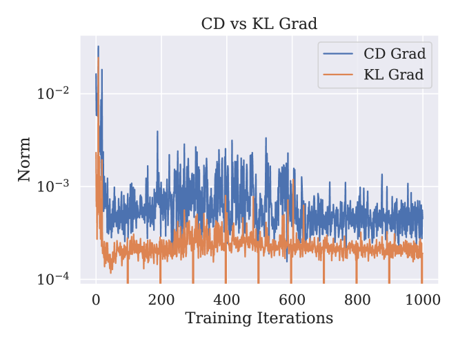
where for brevity, we summarize $\Pi_{\theta}^{t}(p({\bm{x}}))=q_{\theta}({\bm{x}})$. The first two terms are identical to those of Equation 1 and the third gradient term (which we refer to as the KL divergence term) corresponds to minimizing the divergence between $q_{\theta}({\bm{x}})$ and $p_{\theta}({\bm{x}})$. In practice, past contrastive divergence approaches have ignored the third gradient term, which was difficult to estimate and claimed to be empirically negligible (Hinton, 1999) (which in Figure 9 we show to be non-negligible), leading to the incorrect optimization of Equation 2. To correctly optimize Equation 2, we construct a new joint loss expression $\mathcal{L}_{\text{Full}}$, consisting of traditional contrastive loss $\mathcal{L}_{\text{CD}}$ and a new loss expression $\mathcal{L}_{\text{KL}}$, to accurately exhibit all three gradient terms. Specifically, we have $\mathcal{L}_{\text{Full}}=\mathcal{L}_{\text{CD}}+\mathcal{L}_{\text{KL}}$ where $\mathcal{L}_{\text{CD}}$ is

$$\mathcal{L}_{\text{CD}}=\mathbb{E}_{p_{D}({\bm{x}})}[E_{\theta}({\bm{x}})]-\mathbb{E}_{\text{stop\_grad}(q_{\theta}({\bm{x}}^{\prime}))}[E_{\theta}({\bm{x}}^{\prime})],$$ (5)

and the ignored KL divergence term corresponding to the following KL loss:

$$\leavevmode\resizebox{408.68454pt}{}{$\mathcal{L}_{\text{KL}}=\mathbb{E}_{q_{\theta}({\bm{x}})}[E_{\text{stop\_grad}(\theta)}({\bm{x}})]+\mathbb{E}_{q_{\theta}({\bm{x}})}[\log(q_{\theta}({\bm{x}}))]$}.$$ (6)

Despite being difficult to estimate, we show that $\mathcal{L}_{\text{KL}}$ is a useful tool for both speeding up and stabilizing training of EBMs. We provide derivations showing the equivalence of gradients of $\mathcal{L}_{\text{Full}}$ and that of Equation 2 in the appendix, where stop gradient operators are necessary to ensure correct gradients. Figure 2 illustrates the overall effects of both losses. Equation 5 encourage the energy function to assign low energy to real samples and high energy for generated samples. However, only optimizing Equation 5 often leads to an adversarial mode where the energy function learns to simply generate an energy landscape that makes sampling difficult. The KL divergence term counteracts this effect and encourages sampling to closely approximate the underlying distribution $p_{\theta}({\bm{x}})$, by encouraging samples to be both low energy under the energy function as well as diverse. Empirically, we find that including for KL term significantly improves both the stability, generation quality, and robustness to different model architectures (Figure 8). Next, we will discuss our approach towards estimating this KL divergence.

2.2 Estimating the missing gradient term

Estimating $\mathcal{L}_{\text{KL}}$ can further be decomposed into two separate objectives, minimizing the energy of samples from $q_{\theta}({\bm{x}})$, which we refer to as $\mathcal{L}_{\text{opt}}$ (Equation 7) and maximizing the entropy of samples from $q_{\theta}({\bm{x}})$ which we refer to as $\mathcal{L}_{\text{ent}}$ (Equation 8).

Minimizing Sampler Energy. To minimize the energy of samples from $q_{\theta}({\bm{x}})$ we can directly differentiate through both the energy function and MCMC sampling. We follow recent work in EBMs and utilize Langevin dynamics (Du & Mordatch, 2019; Nijkamp et al., 2019b; Grathwohl et al., 2019) for our MCMC transition kernel, and note that each step of Langevin sampling is fully differentiable with respect to underlying energy function parameters. Precisely, gradient of $\mathcal{L}_{\text{opt}}$, $\frac{\partial\mathcal{L}_{\text{opt}}}{\partial\theta}$ becomes

where $\omega\sim\mathcal{N}(0,\lambda)$ and ${\bm{x}}_{i}^{\prime}$ represents the $\text{i}^{\text{th}}$ step of Langevin sampling. To reduce the memory overhead of this differentiation procedure, we only differentiate through the last step of Langevin sampling as also done in (Vahdat et al., 2020). In the appendix we show that this leads to the same effect as differentiation through Langevin sampling.

Entropy Estimation. To maximize the entropy of samples from $q_{\theta}({\bm{x}})$, we use a non-parametric nearest neighbor entropy estimator (Beirlant et al., 1997), which is shown to be mean square consistent (Kozachenko & Leonenko, 1987) with root-n convergence rate (Tsybakov & Van der Meulen, 1996). The entropy $H$ of a distribution $p({\bm{x}})$ can be estimated through a set $X={x_{1},x_{2},\ldots,x_{n}}$ of $n$ different points sampled from $p({\bm{x}})$ as $H(p_{\theta}({\bm{x}}))=\frac{1}{n}\sum_{i=1}^{n}\ln(n\cdot\operatorname{NN}(x_{i},X))+O(1)$ where the function $\operatorname{NN}(x_{i},X)$ denotes the nearest neighbor distance of $x_{i}$ to any other data point in $X$. Based off the above entropy estimator, we write $\mathcal{L}_{\text{ent}}$ as the entropy loss:

$$\mathcal{L}_{\text{ent}}=\mathbb{E}_{q({\bm{x}})}[-\log(\operatorname{NN}({\bm{x}},B))]$$ (8)

where we measure the nearest neighbor with respect to a set $B$ of 100 past samples from MCMC chains. We utilize L2 distance as the metric for computing nearest neighbors. This type of nearest entropy estimator is known to scale poorly to high dimensions (requiring an exponential number of samples to yield an accurate entropy estimate). However, in our setting, we do not need an accurate estimate of entropy. Instead, our computation of entropy is utilized as a fast regularizer to prevent sampling from collapsing.

2.3 Data Augmentation Transitions

Langevin sampling, our MCMC transition kernel, is prone to falling into local probability modes (Neal, 2011). In the image domain, this manifests with sampling chains always converging to a fixed image (Du & Mordatch, 2019). A core difficulty is that distances between two qualitatively similar images can be significantly far away from each other in the input domain, on which sampling is applied. While $\mathcal{L}_{\text{KL}}$ serves as a regularizer to prevent sampling collapse in Langevin dynamics, Langevin dynamics alone is not enough to encourage large jumps in a finite number of steps. It is further beneficial to have an individual sampling chain have the ability to mix between probability modes.

  Input: data dist $p_{D}({\bm{x}})$, step size $\lambda$, number of steps $K$, data augmentation $D(\cdot)$, stop gradient operator $\Omega(\cdot)$, EBM $E_{\theta}(\cdot)$

  $\mathcal{B}\leftarrow\varnothing$

  while not converged do

     ${\bm{x}}^{+}_{i}\sim p_{D}$

     $\tilde{{\bm{x}}}^{0}_{i}\sim\mathcal{B}$ with 99% probability and $\mathcal{U}$ otherwise

     $X\sim\mathcal{B}$ for nearest neighbor entropy calculation

     $\triangleright$ Apply data augmentation to sample:

     $\tilde{{\bm{x}}}^{0}_{i}=D(\tilde{{\bm{x}}}^{0}_{i})$

     $\triangleright$ Generate sample using Langevin dynamics:

     for sample step $k=1$ to $K$ do

        $\tilde{{\bm{x}}}^{k-1}_{i}=\Omega(\tilde{{\bm{x}}}^{k-1}_{i})$

        $\tilde{{\bm{x}}}^{k}\leftarrow\tilde{{\bm{x}}}^{k-1}-\nabla_{\bm{x}}E_{\theta}(\tilde{{\bm{x}}}^{k-1})+\omega,\;\;\omega\sim\mathcal{N}(0,\sigma)$

     end for

     $\triangleright$ Generate two variants of ${\bm{x}}^{-}$ with and without gradient propagation:

     ${\bm{x}}^{-}_{i}=\Omega(\tilde{{\bm{x}}}^{k}_{i})$

     $\hat{{\bm{x}}}^{-}_{i}=\tilde{{\bm{x}}}^{k}_{i}$

     $\triangleright$ Optimize objective $\mathcal{L}_{\text{CD}}+\mathcal{L}_{\text{KL}}$ wrt $\theta$:

     $\mathcal{L}_{\text{CD}}=\frac{1}{N}\sum_{i}(E_{\theta}({\bm{x}}^{+}_{i})-E_{\theta}({\bm{x}}^{-}_{i})$

     $\mathcal{L}_{\text{KL}}=E_{\Omega(\theta)}(\hat{{\bm{x}}}^{-}_{i})-\log(NN(\hat{{\bm{x}}}^{-}_{i},X)$

     $\triangleright$ Optimize objective $\mathcal{L}_{\text{CD}}+\mathcal{L}_{\text{KL}}$ wrt $\theta$:

     $\Delta\theta\leftarrow\nabla_{\theta}(\mathcal{L}_{\text{CD}}+\mathcal{L}_{\text{KL}})$

     Update $\theta$ based on $\Delta\theta$ using Adam optimizer

     $\triangleright$ Update replay buffer $\mathcal{B}$

     $\mathcal{B}\leftarrow\mathcal{B}\cup\tilde{{\bm{x}}}_{i}^{-}$

  end while

Algorithm 1 EBM training algorithm

Figure 3: Illustration of our multi-scale EBM architecture. Our energy function over an image is defined compositionally as the sum of energy functions on different resolutions of an image.

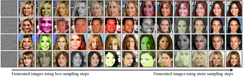
To encourage greater exploration between similar inputs in our model, we propose to augment chains of MCMC sampling with periodic data augmentation transitions that encourages movement between “similar” inputs. In particular, we utilize a combination of color, horizontal flip, rescaling, and Gaussian blur augmentations. Such combinations of augmentation has recently seen success applied in unsupervised learning (Chen et al., 2020). Specifically, during training time, we initialize MCMC sampling from a data augmentation applied to an input sampled from the buffer of past samples. At test time, during the generation, we apply a random augmentation to the input after every 20 steps of Langevin sampling. We illustrate this process in the bottom of Figure 2. Data augmentation transitions are always taken.

2.4 Compositional Multi-scale Generation

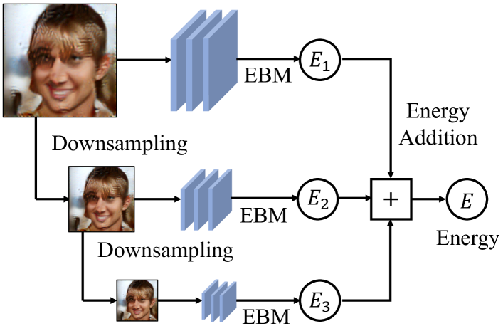
To encourage energy functions to focus on features in both low and high resolutions, we define our energy function as the composition (sum) of a set of energy functions operating on different scales of an image, illustrated in Figure 3. Since the downsampling operation is fully differentiable, Langevin based sampling can be directly applied to the energy function. In our experiments, we utilize full, half, and quarter resolution image as input and show that this improves the generation performance.

  Input: number of data augmentation applications $N$, step size $\lambda$, number of steps $K$, data augmentation $D(\cdot)$, EBM $E_{\theta}(\cdot)$

  $\tilde{{\bm{x}}}^{0}\sim\mathcal{U}$

  $\triangleright$ Generate samples through $N$ iterative steps of data augmentation/Langevin dynamics:

  for sample step $n=1$ to $N$ do

     $\triangleright$ Apply data augmentation to samples:

     $\tilde{{\bm{x}}}^{0}=D(\tilde{{\bm{x}}}^{0}_{i})$

     $\triangleright$ Run $K$ steps of Langevin dynamics:

     for sample step $k=1$ to $K$ do

        $\tilde{{\bm{x}}}^{k}\leftarrow\tilde{{\bm{x}}}^{k-1}-\nabla_{\bm{x}}E_{\theta}(\tilde{{\bm{x}}}^{k-1})+\omega,\;\;\omega\sim\mathcal{N}(0,\sigma)$

     end for

     $\triangleright$ Iteratively refine samples:

     $\tilde{{\bm{x}}}^{0}=\tilde{{\bm{x}}}^{k}$

  end for

  $\triangleright$ Final output:

  ${\bm{x}}=\tilde{{\bm{x}}}^{0}$

Algorithm 2 EBM sampling algorithm

2.5 Training Algorithm and Sampling

We provide an overview of our overall proposed training algorithm in Algorithm 1. Our overall approach is similar to the algorithm presented in (Du & Mordatch, 2019), with two notable differences. First, we apply data augmentation to samples drawn for the replay buffer. Second, we propagate gradients through sampling to efficiently compute $\mathcal{L}_{\text{KL}}$. We further present the sample generation algorithm for a trained EBMs in Algorithm 2. We iteratively apply $N$ steps of data augmentation and Langevin sampling to mimic the replay buffer utilized during training.

3 Experiments

We perform empirical experiments to validate the following set of questions: (1) What are the effects of each proposed component towards training EBMs? (2) Are our trained EBMs able to perform well on downstream applications of EBMs, such as image generation, out-of-distribution detection, and concept compositionality?

3.1 Experimental Setup

We investigate the efficacy of our proposed approach. Models are trained using the Adam Optimizer (Kingma & Ba, 2015), on a single 32GB Volta GPU for CIFAR-10 for 1 day, and for 3 days on 8 32GB Volta GPUs for CelebaHQ, LSUN and ImageNet 32x32 datasets. We provide detailed training configuration details in the appendix.

Our improvements are largely built on top of the EBMs training framework proposed in (Du & Mordatch, 2019). We use a buffer size of 10000, with a resampling rate of 0.1%. Our approach is significantly more stable than IGEBM, allowing us to remove aspects of regularization in (Du & Mordatch, 2019). We remove the clipping of gradients in Langevin sampling as well as spectral normalization on the weights of the network. In addition, we add self-attention blocks and layer normalization blocks in residual networks of our trained models. In multi-scale architectures, we utilize 3 different resolutions of an image, the original image resolution, half the image resolution and a quarter the image resolution. We report detailed architectures in the appendix. When evaluating models, we utilize the EMA model with EMA weight of 0.9999.

Table 1: Table of Inception and FID scores for generations of CIFAR-10, CelebA-HQ and ImageNet32x32 images. All others numbers are taken directly from corresponding papers. On CIFAR-10, our approach outperforms past EBM approaches and achieves performance close to SNGAN. On CelebA-HQ, our approach achieves performance close to that of SSGAN. On ImageNet 32x32, our approach achieves similar performance to the PixelIQN (large) model with around one tenth the parameters.

Model	Inception	FID
CIFAR-10 Unconditional
PixelCNN (Van Oord et al., 2016)	4.60	65.9
Multigrid EBM (Gao et al., 2018)	6.56	40.1
IGEBM (Ensemble) (Du & Mordatch, 2019)	6.78	38.2
Short-Run EBM (Nijkamp et al., 2019b)	6.21	44.5
DCGAN (Radford et al., 2016)	6.40	37.1
WGAN + GP (Gulrajani et al., 2017)	6.50	36.4
NCSN (Song & Ermon, 2019)	8.87	25.3
Ours	7.85	25.1
SNGAN (Miyato et al., 2018)	8.22	21.7
SSGAN (Chen et al., 2019)	-	19.7
CelebA-HQ 128x128 Unconditional
Ours	-	28.78
SSGAN (Chen et al., 2019)	-	24.36
ImageNet 32x32 Unconditional
PixelCNN (van den Oord et al., 2016)	7.16	40.51
PixelIQN (small) (Ostrovski et al., 2018)	7.29	37.62
PixelIQN (large) (Ostrovski et al., 2018)	8.69	26.56
IGEBM (Du & Mordatch, 2019)	5.85	62.23
Ours	8.73	32.48

Figure 4: Randomly selected unconditional 128x128 CelebA-HQ images generated from our trained EBM model. Samples are relatively diverse with limited artifacts.

Figure 5: Visualization of Langevin dynamics sampling chains on an EBM trained on CelebA-HQ 128x128. Samples travel between different modes of images. Each consecutive images represents 30 steps of sampling, with data augmentation transitions every 60 steps.

3.2 Image Generation

Figure 6: Output samples after running Langevin dynamics from a fixed initial sample (center of square), with or without intermittent data-augmentation transitions. Without data-augmentation transitions, all samples converge to same image, while data augmentations enables chains to seperate.

Figure 7: Illustration of very low temperature samples from our model with KL loss and data augmentation compared to those from IGEBM on CIFAR-10 (left) and CelebA-HQ (right). After a large number of sampling steps, IGEBM converges to stranges hues in CIFAR-10 and random textures on CelebA-HQ. In contrast, due to better mode exploration, adding both improvements maintains naturalistic image modes on both CIFAR-10 and CelebA-HQ.

Figure 8: The KL loss significantly improves the stability of EBM training. Stable EBM training occurs when the energy difference (illustrated in bottom row) is roughly zero. We find that without using the KL loss term (left column), EBM training quickly diverges (bottom left). Spectral normalization prevents divergence of energies, but cannot be combined with self attention without destabilizing training. KL loss (right column) maintains an energy differences to 0 (bottom right), even with the addition of self attention. Inception scores rapidly rises with KL loss (top right), but fall without KL loss (top left) due to destabilized training. Spectral norm prevents the Inception score from falling, but the score also does not increase much due to constraints in the architecture.

We evaluate our approach on CIFAR-10, Imagenet 32x32 (Deng et al., 2009), and CelebA-HQ (Karras et al., 2017) datasets. Additional quantitative comparisons, results, and ablations can be found in the appendix of the paper.

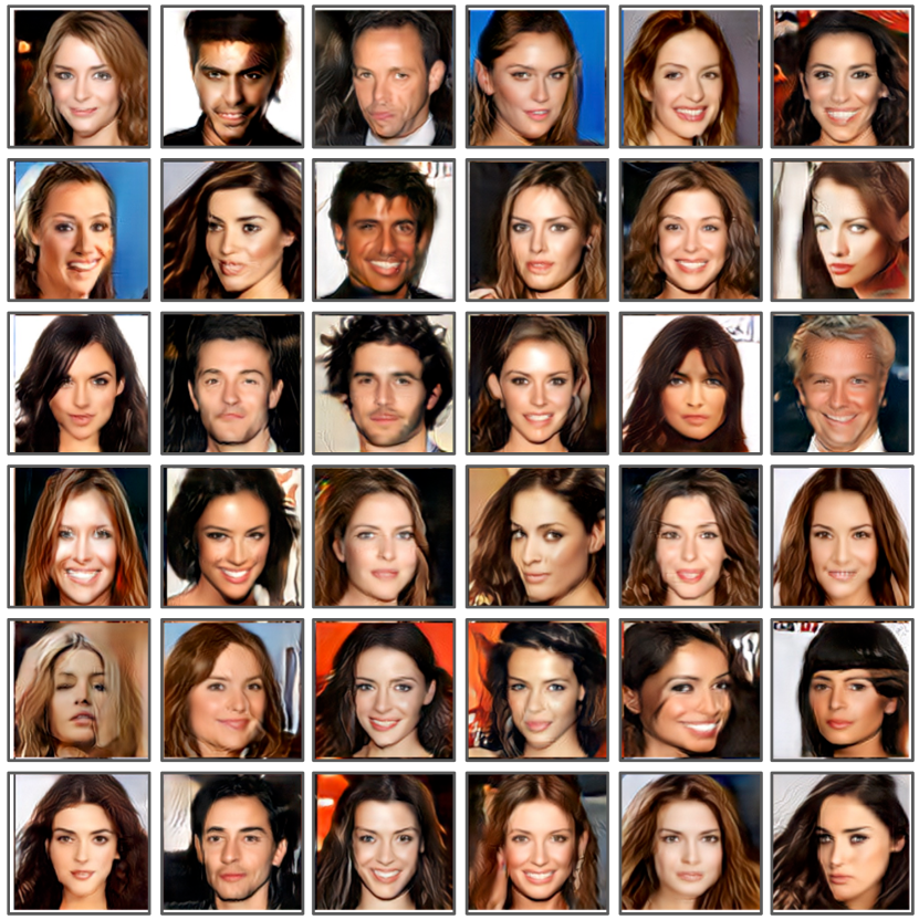
Image Quality. We evaluate our approach on unconditional generation in Table 1. We utilize Inception (Salimans et al., 2016) and FID (Heusel et al., 2017) implementations from (Du & Mordatch, 2019) to evaluate samples. On CIFAR-10, we find that our approach outperforms many past EBM approaches in both FID and Inception scores using a similar number of parameters. We find that our performance is slightly worse than that of SNGAN and SSGAN. On CelebA-HQ, we find that our approach outperforms our reimplementation of SNGAN using default ImageNet hyperparameters, and is close to the reported numbers of SSGAN. Finally, on Imagenet32x32, we find that our approach outperforms previous EBM models and achieves performance comparable to that of the large PixelIQN model in terms of FID and Inception score. We note, however, that our model is significantly smaller than the PixelIQN model and has one tenth the number of parameters. We present example qualitative images from CelebA-HQ in Figure 4 and present qualitative images on other datasets in the appendix of the paper. While our overall generative performance are not the best reported, we emphasize that it improves existing generative performance of EBMs, which have unique benefits such as compositionality (Section 3.4).

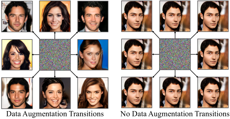
Effect of Data Augmentation. We evaluate the effect of data augmentation on sampling in EBMs. In Figure 5 we show that by combining Langevin sampling with data augmentation transitions, we are able to enable chains to mix across different images, whereas prior works have shown Langevin converging to fixed images. In Figure 6 we show that given a fixed random noise initialization, data augmentation transitions enable to reach a diverse number of different samples, while sampling without data augmentation transitions leads all chains to converge to the same face.

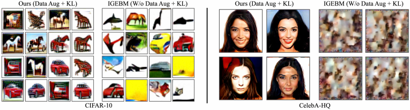
Mode Convergence. We further investigate high likelihood modes of our model. In Figure 7, we compare very low energy samples (obtained after running gradient descent 1000 steps on an energy function) for both our model with data augmentation and KL loss and the IGEBM model. Due to improved mode exploration, we find that low temperature samples under our model with data augmentation/KL loss reflect typical high likelihood ”modes” in the training dataset, while our baseline models converges to odd shapes, also noted in (Nijkamp et al., 2019a).

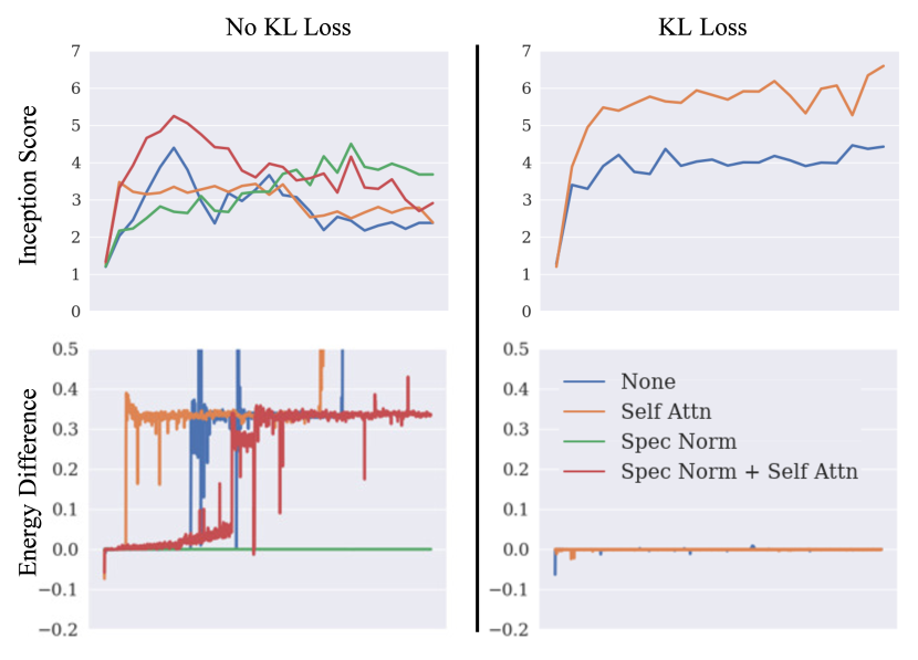
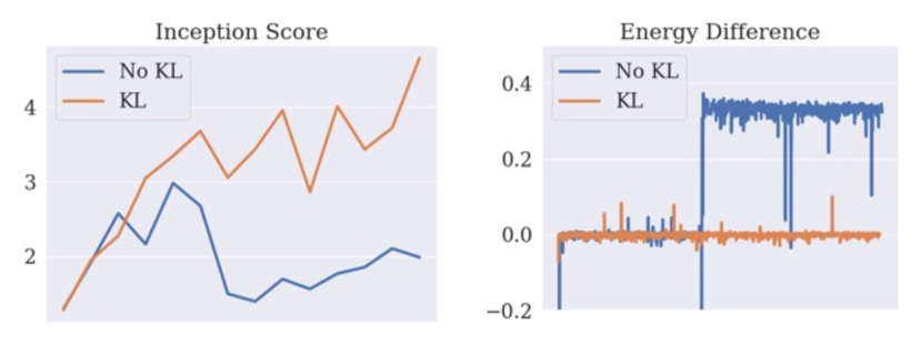
Stability/KL Loss. EBMs are difficult to train and are sensitive to both the exact architecture and to various hyper-parameters. We found that the addition of a KL term into our training objective significantly improved the stability of training, by encouraging the sampling distribution to match the model distribution. In Figure 8, we measure training stability by measuring the energy differences between real and generated images. Stable training occurs when the energy difference is close to zero. Without $\mathcal{L}_{\text{KL}}$, we found that training our model with or without self-attention were both unstable, with differences spiking. Adding spectral normalization stabilizes training, but the addition of self-attention once again destabilizes training. In contrast with $\mathcal{L}_{\text{KL}}$, the addition of self-attention is also stable. We further compare Inception scores in Figure 8 over training and find that while spectral normalization stabilizes training, it does at the expense of decreased improvement of Inception score.

The addition of the KL term itself is not too expensive, simply requiring an additional nearest neighbor computation during training, a relatively insignificant cost compared to the number of negative sampling steps used during training. With a intermediate number of negative sampling steps (60 steps) during training, adding the KL term incurs a roughly 20% computational cost. This difference is further decreased with a larger number of sampling steps.

Ablations. We ablate each portion of our proposed approach in Table 2. We find that each our proposed components have significant gains in generation performance. In particular, we find a large gain in overall generative performance when adding the KL loss. This is in part due to a large boost in training stability (Figure 8), enabling significantly longer training times with both multiscale sampling and data augmentation.

Table 2: Ablations of each proposed component on CIFAR-10 generation as well as corresponding stability of training. KL Loss significantly stabilizes EBM training, and enables larges boosts in generation performance via longer training.

KL Loss	KL Loss	Data	Multiscale	Inception	FID	Stability
$\mathcal{L}_{\text{opt}}$	$\mathcal{L}_{\text{ent}}$	Aug	Sampling	Score
No	No	No	No	3.57	169.74	No
No	No	Yes	No	5.13	133.84	No
No	No	Yes	Yes	6.14	53.78	No
Yes	No	Yes	Yes	6.79	32.67	Yes
Yes	Yes	Yes	Yes	7.85	25.08	Yes

KL Gradient. We plot the overall gradient magnitudes of $\mathcal{L}_{\text{CD}}$ and $\mathcal{L}_{\text{KL}}$ when training an EBM on CIFAR-10 in Figure 9. We find that relative magnitude of gradients of both training objectives remains constant across training, and that the gradient of the KL objective is non-negligible.

Figure 9: Plots of the gradient magnitude of ${\mathcal{L}}_{\text{KL}}$ and ${\mathcal{L}}_{\text{CD}}$ across training iterations. Influences and relative magnitude of both loss terms stays constant through training.

Table 3: Table of AUROC values in out-of-distribution detection on unconditional models trained on CIFAR-10 using $\log(p_{\theta}(x))$. Our approach performs the best out of all methods. *JEM is not directly comparable as it uses supervised labels.

Model	PixelCNN++	Glow	IGEBM	JEM*	VERA	Ours
SVHN	0.32	0.24	0.63	0.67	0.83	0.91
Textures	0.33	0.27	0.48	0.60	-	0.88
CIFAR10 Interp	0.71	0.51	0.70	0.65	0.86	0.65
CIFAR100	0.63	0.55	0.50	0.67	0.73	0.83
Average	0.50	0.39	0.57	0.65	-	0.82

3.3 Out of Distribution Robustness

Energy-Based Models (EBMs) have also been shown to exhibit robustness to both out-of-distribution and adversarial samples (Du & Mordatch, 2019; Grathwohl et al., 2019, 2020a). We evaluate out-of-distribution detection of our trained energy function through log-likelihood using the AUROC evaluation metrics proposed in Hendrycks & Gimpel (2016). We similarly evaluate out-of-distribution detection of an unconditional CIFAR-10 model.

Results. We present out-of-distribution results in Table 3, comparing with both likelihood models and EBMs using log-likelihood to detect outliers. We find that our approach significantly outperforms other baselines, with the exception of CIFAR-10 interpolations. We note the JEM (Grathwohl et al., 2019) further requires supervised labels to train the energy function, which has to shown to improve out-of-distribution performance. We posit that by more efficiently exploring modes of the energy distribution at training time, we are able to reduce the spurious modes of the energy function and thus improve out-of-distribution performance.

Table 4: Table of compositional generation accuracy across different models trained on the CelebA-HQ dataset. Generation accuracy measured through attribute predictions using a Resnet-18 classifier is trained to regress young, female, smiling, and wavy hair attributes in CelebA-HQ. Our approach achieves best performance.

Model	Young	Female	Smiling	Wavy
JVAE (Young)	0.543	-	-	-
JVAE (Young $\&$ Female)	0.440	0.554	-	-
JVAE (Young $\&$ Female $\&$ Smiling)	0.488	0.520	0.526
JVAE (Young $\&$ Female $\&$ Smiling $\&$ Wavy)	0.416	0.584	0.561	0.416
IGEBM (Young)	0.506	-	-	-
IGEBM (Young $\&$ Female)	0.367	0.160	-	-
IGEBM (Young $\&$ Female $\&$ Smiling)	0.604	0.648	0.625	-
IGEBM (Young $\&$ Female $\&$ Smiling $\&$ Wavy)	0.550	0.545	0.445	0.781
Ours (Young)	0.847	-	-	-
Ours (Young $\&$ Female)	0.770	0.583	-	-
Ours (Young $\&$ Female $\&$ Smiling)	0.906	0.718	0.968	-
Ours (Young $\&$ Female $\&$ Smiling $\&$ Wavy)	0.922	0.625	0.843	0.906

Figure 10: Examples of EBM compositional generations across different object attributes. Our model is successfully able to compose attributes and is able to construct high resolution, globally coherent compositional renderings, including fine detail such as lighting and reflections.

Figure 11: Qualitative comparisons of compositionality on CelebA-HQ faces. Our approach generates much more realistic looking faces than IGEBM (Du & Mordatch, 2019) and JVAE (Vedantam et al., 2018), with each conditioned attribute.

3.4 Compositionality

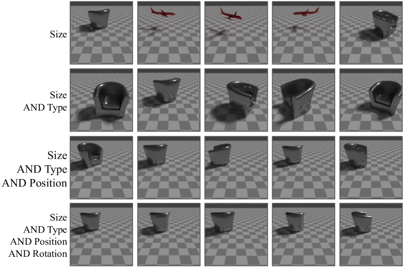
Energy-Based Models (EBMs) have the ability to compose with other models at generation time (Hinton, 1999; Haarnoja et al., 2017; Du et al., 2020a). We investigate to what extent EBMs trained under our new framework can also exhibit compositionality. See (Du et al., 2020a) for a discussion of various compositional operators and applications in EBMs. In particular, we train independent EBMs $E({\bm{x}}|c_{1})$, $E({\bm{x}}|c_{2})$, $E({\bm{x}}|c_{3})$, that learn conditional generative distribution over concept factors $c$ such as facial expression. We test whether we can compose independent energy functions together to generate images with each concept factor simultaneously. We test compositions on the CelebA-HQ dataset, where we train separate EBMs on face attributes of age, gender, smiling, and wavy hair and on a rendered Blender dataset where we train separate EBMs on object attributes of size, position, rotation, and identity.

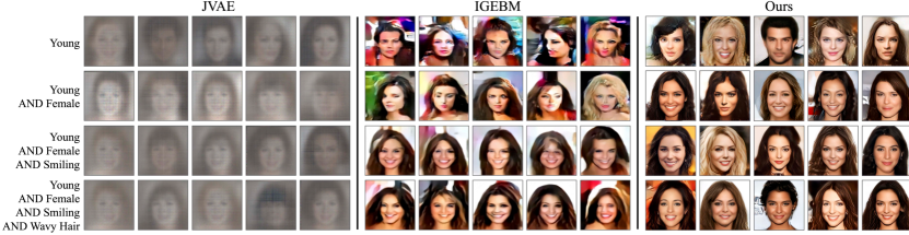
Qualitative Results. We present qualitative results on compositions of energy functions on CelebA-HQ in Figure 11. We consider compositional generation on the factors of young, female, smiling, and wavy hair. Compared to baselines, our approach is able to successfully generate images with each of conditioned factor, with faces being significantly higher resolution than baselines. In Figure 10, we further consider compositions of energy functions over object attributes. We consider compositional generation on factors of size, type, position, and rotation. Again, we find that each associated image generation exhibits the corresponding conditioned attribute. Images are further visually consistent in terms of lighting, shadows and reflections. We note that different from most past work, generations of these combinations of different factors are only specified at generation time, with models being trained independently. Our results indicate that our framework for training EBMs is a promising direction for high resolution compositional visual generation.

Quantitative Comparison. We quantitatively compare compositional generations of our model with IGEBM and JVAE (Vedantam et al., 2018) models on the CelebA-HQ dataset. We assess the compositional generation accuracy of different models by measuring the accuracy with which a pretrained ResNet18 classifier can recover the underlying conditioned attributes. In Table 4, we find that our model has significantly higher attribute recovery compared to baselines across all compositions of attributes.

4 Related Work

Our work is related to a large, growing body of work on different approaches for training EBMs. Our approach is based on contrastive divergence (Hinton, 2002), where an energy function is trained to contrast negative samples drawn from a model distribution and from real data. In recent years, such approaches have been applied to the image domain (Salakhutdinov & Hinton, 2009; Xie et al., 2016; Gao et al., 2018; Du & Mordatch, 2019). (Gao et al., 2018) also proposes a multiscale approach towards generating images from EBMs, but different from our work, uses each sub-scale EBM to initialize the generation of the next EBM, while we jointly sample across each resolution. Our work builds on existing works, and aims to provide improvements in generation and stability.

A difficulty with contrastive divergence training is negative sample generation. To sidestep this issue, a separate line of work utilizes an auxiliary network to amortize the negative portions of the sampling procedure (Kim & Bengio, 2016; Kumar et al., 2019; Han et al., 2019; Xie et al., 2018a; Song & Ou, 2018; Dai et al., 2019; Che et al., 2020; Grathwohl et al., 2020a; Arbel et al., 2020). One line of work (Kim & Bengio, 2016; Kumar et al., 2019; Song & Ou, 2018), utilizes a separate generator network for negative image sample generations. In contrast, (Xie et al., 2018a), utilizes a generator to warm start generations for negative samples and (Han et al., 2019) minimizes a divergence triangle between three models. While such approaches enable better qualitative generation, they also lose some of the flexibility of the EBM formulation. For example, separate energy models can no longer be composed together for generation.

In addition, other approaches towards training EBMs seek instead to investigate separate objectives to train the EBM. One such approach is score matching, where the gradients of an energy function are trained to match the gradients of real data (Hyvärinen, 2005; Song & Ermon, 2019), or with a related denoising (Sohl-Dickstein et al., 2015; Saremi et al., 2018; Ho et al., 2020) approach. Additional objectives include noise contrastive estimation (Gao et al., 2020), learned Steins discrepancy (Grathwohl et al., 2020b), and learned F divergences (Yu et al., 2020).

Most prior work in contrastive divergence has ignored the KL term (Hinton, 1999; Salakhutdinov & Hinton, 2009). A notable exception is (Ruiz & Titsias, 2019), which obtains a similar KL divergence term to ours. Ruiz & Titsias (2019) use a high variance REINFORCE estimator to estimate the gradient of the KL term, while our approach relies on auto-differentiation and nearest neighbor entropy estimators. Differentiation through model generation procedures has previously been explored in other models (Finn & Levine, 2017; Metz et al., 2016). Other related entropy estimators include those based on Stein’s identity (Liu et al., 2017) and MINE (Belghazi et al., 2018). In contrast to these approaches, our entropy estimator relies only on nearest neighbor calculation, and does not require the training of an independent neural network.

5 Conclusion

We propose a simple and general framework for improving generation and ease of training of EBMs. We show that the framework enables high resolution compositional image generation and out-of-distribution robustness. In the future, we are interested in further computational scaling of our framework and its applications to additional domains such as text, video, and reasoning.

6 Acknowledgements

We would like to thank Jasha Sohl Dickstein, Bo Dai, Rif Sauros, Simon Osindero, Alex Alemi and anonymous reviewers for there helpful feedback on initial versions of the manuscript. Yilun Du is supported by a NSF GFRP fellowship. This work is in part supported by ONR MURI N00014-18-1-2846 and IBM Thomas J. Watson Research Center CW3031624.

In this supplement, we present additional image generation results in Section A. Next we detail experimental settings in Section B. We provide derivations of gradients of $\mathcal{L}_{\text{CD}}$ and $\mathcal{L}_{\text{KL}}$ and show there equivalence to the original contrastive divergence objective in Section C. Finally we provide additional analysis of our method in Section D.

Appendix A More Image Results

A.1 Nearest Neighbor Generations

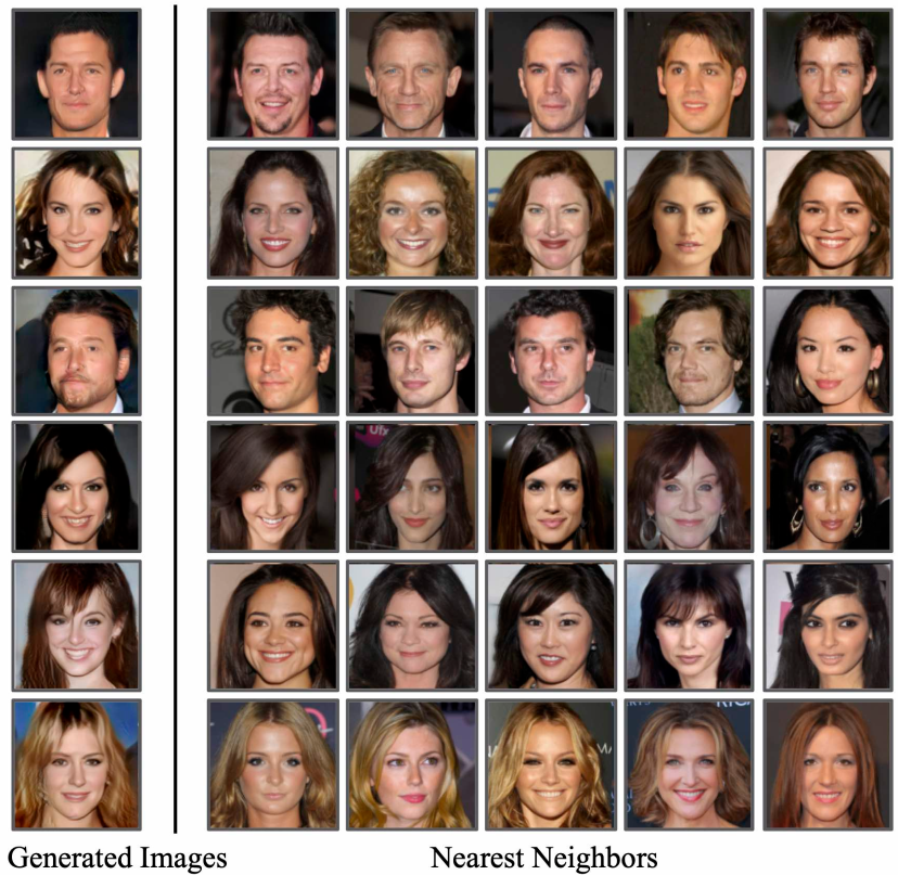
We present L2 nearest neighbors in CelebA-HQ training dataset of unconditional image samples from our trained EBM in Figure 13. We find that our approach generates images distinct from the training set.

A.2 Additional Quantitative Results

We further quantitatively compare our generations with those of SNGAN on LSUN 128x128 bedroom scenes. We find that an SNGAN model trained on LSUN 128x128 bedroom scenes obtains an FID of 64.05 compared to our approach, which obtains an FID of 33.46. To report SNGAN scores, we re-implemented the SNGAN model using the default hyper parameters to train models on ImageNet 128x128.

A.3 Additional Qualitative Images

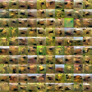
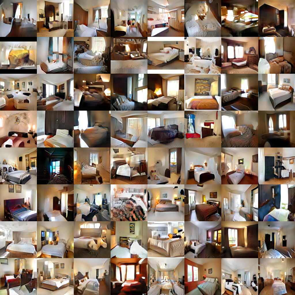
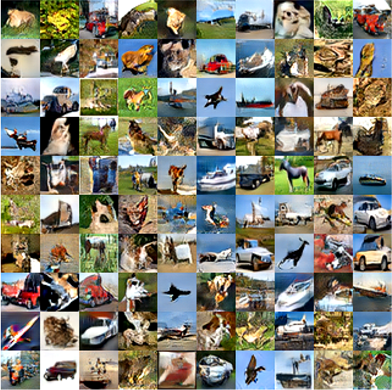
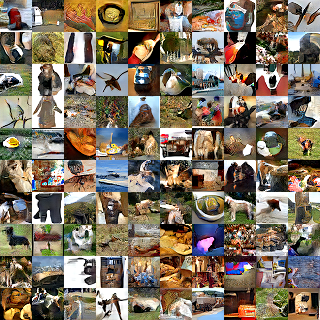
We present qualitative visualizations of unconditional samples generated from an EBM. Figure 14 shows unconditional image generations from LSUN bedroom scenes. Figure 15 shows unconditional image generations on the CIFAR-10 dataset. Finally, Figure 16 shows unconditional image generations on the ImageNet 32x32 dataset. In all three different settings, we find that our generated unconditional images are relatively globally coherent.

Appendix B Training Details

B.1 Model Architectures

In this part, we provide the model architectures used in our experiments. When training multiscale energy functions, our final output energy function is the sum of energy functions applied to the full resolution image, the half resolution image, and the quarter resolution image. We use the architecture reported in Table D.3 for the full resolution image on CIFAR-10 and ImageNet 32x32 (used in the main paper Section 3.2 and 3.3). The model architecture used on the CelebA-HQ and LSUN datasets are reported in Table D.3 (used in the main paper Section 3.2 and 3.4). The half-resolution models share the architecture listed in Table D.3, but with the first down-sampled residual block removed. Similarly, the quarter resolution models share the architectures listed, but with the first two down-sampled residual blocks removed. We utilize group normalization (Wu & He, 2018) inside each residual block and utilize the Swish nonlinearity (Ramachandran et al., 2018).

B.2 Experiment Configurations For Different Datasets

CIFAR-10/ImageNet 32x32.  For CIFAR-10 and ImageNet 32x32, we use 40 steps of Langevin sampling to generate a negative sample. The Langevin sampling step size is set to be 500, with Gaussian noise of magnitude 0.001 at each iteration. The data augmentation transform consists of color augmentation of strength 1.0 from (Chen et al., 2020), a random horizontal flip, and a image resize between 0.02 and 1.0. This is used in the main paper Section 3.2 and 3.3.

CelebA/LSUN Bedroom.  For the CelebA-HQ and LSUN bed datasets, we use 40 steps of Langevin sampling to generate negative samples. The Langevin sampling step size is set to be 1000, with Gaussian noise of magnitude 0.001 applied at each iteration. The data augmentation transform consists of color augmentation of strength 1.0 from (Chen et al., 2020), a random horizontal flip, and a image resize between 0.08 and 1.0. This is used in the main paper Section 3.2 and 3.4.

Appendix C Loss Gradient Derivation

We show that the gradient of the contrastive divergence objective, $\mathcal{L}_{\text{CD\_Full}}$ is equivalent to that of the $\mathcal{L}_{\text{Full}}=\mathcal{L}_{\text{KL}}+\mathcal{L}_{\text{CD}}$. Recall that the contrastive divergence objective is given by

$$\mathcal{L}_{\text{CD\_Full}}=\text{KL}(p_{D}({\bm{x}})\;||\;p_{\theta}({\bm{x}}))-\text{KL}(q_{\theta}({\bm{x}})\;||\;p_{\theta}({\bm{x}})).$$ (9)

The gradient of the first KL term with respect to $\theta$, $\frac{\partial\text{KL}(p_{D}({\bm{x}})\;||\;p_{\theta}({\bm{x}}))}{\partial\theta}$ is

while the gradient of the second KL term with respect to $\theta$, $\frac{\text{KL}(q_{\theta}({\bm{x}})\;||\;p_{\theta}({\bm{x}}))}{\partial\theta}$

with the overall gradient being

$$\leavevmode\resizebox{375.80542pt}{}{$\begin{split}\frac{\mathcal{L}_{\text{CD\_Full}}}{\partial\theta}=-(\mathbb{E}_{p_{D}({\bm{x}})}\left[\frac{\partial E_{\theta}({\bm{x}})}{\partial\theta}\right]&-\mathbb{E}_{q_{\theta}({\bm{x}}^{\prime})}[\frac{\partial E_{\theta}({\bm{x}}^{\prime})}{\partial\theta}]\\ &+{\color[rgb]{1,0,0}\definecolor[named]{pgfstrokecolor}{rgb}{1,0,0}\frac{\partial q({\bm{x}}^{\prime})}{\partial\theta}\frac{\partial\text{KL}(q_{\theta}({\bm{x}}^{\prime})\;||\;p_{\theta}({\bm{x}}^{\prime}))}{\partial q_{\theta}({\bm{x}}^{\prime})})}\end{split}$}.$$ (12)

We have that

$$\mathcal{L}_{\text{CD}}=\mathbb{E}_{p_{D}({\bm{x}})}[E_{\theta}({\bm{x}})]-\mathbb{E}_{\text{stop\_grad}(q_{\theta}({\bm{x}}^{\prime}))}[E_{\theta}({\bm{x}}^{\prime})],$$ (13)

with corresponding gradients

$$\leavevmode\resizebox{375.80542pt}{}{$\frac{\partial\mathcal{L}_{\text{CD}}}{\partial\theta}=\mathbb{E}_{p_{D}({\bm{x}})}\left[\frac{\partial E_{\theta}({\bm{x}})}{\partial\theta}\right]-\mathbb{E}_{q_{\theta}({\bm{x}}^{\prime})}[\frac{\partial E_{\theta}({\bm{x}}^{\prime})}{\partial\theta}]$}.$$ (14)

Furthermore, we have that

$$\mathcal{L}_{\text{KL}}=\mathbb{E}_{q_{\theta}({\bm{x}})}[E_{\text{stop\_grad}(\theta)}({\bm{x}})]+\mathbb{E}_{q_{\theta}({\bm{x}})}[\log(q_{\theta}({\bm{x}}))],$$ (15)

can be rewritten as

$$\mathcal{L}_{\text{KL}} =\mathbb{E}_{q_{\theta}({\bm{x}})}[-\log(p_{\theta}(x))]+\mathbb{E}_{q_{\theta}({\bm{x}})}[\log(q_{\theta}({\bm{x}}))]$$ (16)

$$=\text{KL}(q_{\theta}({\bm{x}})\;||\;p_{\text{stop\_gradient}(\theta)}({\bm{x}})).$$ (17)

The corresponding gradient of the objective is

$$\frac{\partial\mathcal{L}_{\text{KL}}}{\partial\theta}=\frac{\partial q({\bm{x}})}{\partial\theta}\frac{\partial\text{KL}(q_{\theta}({\bm{x}})\;||\;p_{\theta}({\bm{x}}))}{\partial q_{\theta}({\bm{x}})}.$$ (18)

Thus the sum of the gradients in $\frac{\partial\mathcal{L}_{\text{CD}}}{\partial\theta}$ (Equation 14) and $\frac{\partial\mathcal{L}_{\text{KL}}}{\partial\theta}$ (Equation 18) is equal to the full contrastive divergence gradient $\frac{\mathcal{L}_{\text{CD\_Full}}}{\partial\theta}$ ( Equation 12).

Appendix D Additional Analysis

D.1 Alternative Sampling Distributions

Instead of utilizing $q_{\theta}({\bm{x}})$ as $\Pi_{\theta}^{t}(p_{D}({\bm{x}}))$, as noted in the method section, our approach can further maximize likelihood as long as $\text{KL}(p_{D}({\bm{x}})\;||\;p_{\theta}({\bm{x}}))$ is greater $\text{KL}(q_{\theta}({\bm{x}})\;||\;p_{\theta}({\bm{x}}))$. We test an alternative sampler $q_{\theta}({\bm{x}})$ consisting of initializing Langevin dynamics from random noise in Figure 12. We find again that our approach improves the training stability.

Figure 12: Inception Score and energy difference plots when $\mathcal{L}_{\text{KL}}$ is applied to MCMC initialized from random noise.

D.2 Analysis of Truncated Langevin Backpropagation

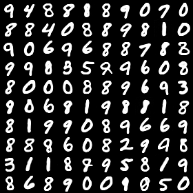
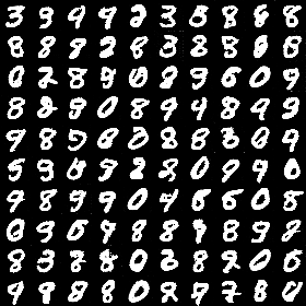
To better understand the training effect of $\mathcal{L}_{\text{KL}}$, we analyze the effect of truncating backpropogation through Langevin sampling. We train two separate models on MNIST, one with backpropogation through all Langevin steps, and one with backpropogation through only the last Langevin step. We obtain an FID of 90.54 with backpropogation through only 1 step of Langevin sampling and an FID of 94.85 with backpropogation through all steps of Langevin sampling. We present illustrations of samples generated with one step in Figure 17 and with all steps in Figure 18. Overall, we find little degradation in performance with the truncation of backpropogation, but note that backpropogation through all steps of sampling is over 3 times slower to train.

D.3 Analysis of Effect of KL Loss on Mode Sampling

We illustrate the effect of $\mathcal{L}_{\text{KL}}$ as a regularizer to prevent EBM sampling collapse. When training an EBM, $\mathcal{L}_{\text{KL}}$ serves as a repelling term encouraging MCMC samples from an EBM to both have low energy and exhibit diversity. In the absence of $\mathcal{L}_{\text{KL}}$, we find that EBM sampling always collapses and eventually always generates samples illustrated in Figure 19. These samples are significantly less diverse than those generated when training with $\mathcal{L}_{\text{KL}}$ ( Figure D.3), which never suffers from sampling collapse.

Figure 13: Nearest neighbors in the L2 space of generated images in CelebA-HQ 128x128.

Figure 14: Randomly selected unconditional LSUN bed 128x128 samples from our trained EBM.

Figure 15: Randomly selected unconditional CIFAR-10 samples from our trained EBM.

Figure 16: Randomly selected unconditional ImageNet 32x32 samples from our trained EBM.

Table 5: The model architecture used for CIFAR-10 and ImageNet-32x32 experiments.

3x3 conv2d, 64
ResBlock 64
ResBlock Down 64
ResBlock 64
ResBlock Down 64
Self Attention 64
ResBlock 128
ResBlock Down 128
ResBlock 256
ResBlock Down 256
Global Mean Pooling
Dense $\rightarrow$ 1

Table 6: The model architecture used for CelebA-HQ/LSUN room experiments.

3x3 conv2d, 64
ResBlock Down 64
ResBlock Down 128
ResBlock Down 128
ResBlock 256
ResBlock Down 256
Self Attention 512
ResBlock 512
ResBlock Down 512
Global mean Pooling
Dense $\rightarrow$ 1

Figure 17: Generations on MNIST with backpropogation through 1 step of Langevin sampling.

Figure 18: Generations on MNIST with backpropogation through all steps of Langevin sampling.

Figure 19: Illustration of collapsed sampling from an EBM. Sampling does not collapse with the addition of the KL loss.

References

- Arbel et al. (2020) Michael Arbel, Liang Zhou, and Arthur Gretton. Generalized energy based models. arXiv preprint arXiv.org/abs/2003.05033, 2020.
- Bartunov et al. (2019) Sergey Bartunov, Jack W Rae, Simon Osindero, and Timothy P Lillicrap. Meta-learning deep energy-based memory models. arXiv preprint arXiv:1910.02720, 2019.
- Beirlant et al. (1997) Jan Beirlant, E. Dudewicz, L. Gyor, and E.C. Meulen. Nonparametric entropy estimation: An overview. International Journal of Mathematical and Statistical Sciences, 6, 01 1997.
- Belghazi et al. (2018) Mohamed Ishmael Belghazi, Aristide Baratin, Sai Rajeswar, Sherjil Ozair, Yoshua Bengio, Aaron Courville, and R Devon Hjelm. Mine: mutual information neural estimation. arXiv preprint arXiv:1801.04062, 2018.
- Che et al. (2020) Tong Che, Ruixiang Zhang, Jascha Sohl-Dickstein, Hugo Larochelle, Liam Paull, Yuan Cao, and Yoshua Bengio. Your gan is secretly an energy-based model and you should use discriminator driven latent sampling. arXiv preprint arXiv.org/abs/2003.06060, 2020.
- Chen et al. (2019) Ting Chen, Xiaohua Zhai, Marvin Ritter, Mario Lucic, and Neil Houlsby. Self-supervised gans via auxiliary rotation loss. In Proceedings of the IEEE Conference on Computer Vision and Pattern Recognition, pp. 12154–12163, 2019.
- Chen et al. (2020) Ting Chen, Simon Kornblith, Mohammad Norouzi, and Geoffrey Hinton. A simple framework for contrastive learning of visual representations. arXiv preprint arXiv:2002.05709, 2020.
- Dai et al. (2019) Bo Dai, Zhen Liu, Hanjun Dai, Niao He, Arthur Gretton, Le Song, and Dale Schuurmans. Exponential family estimation via adversarial dynamics embedding. In Advances in Neural Information Processing Systems, pp. 10979–10990, 2019.
- Deng et al. (2009) Jia Deng, Wei Dong, Richard Socher, Li-Jia Li, Kai Li, and Li Fei-Fei. Imagenet: A large-scale hierarchical image database. In CVPR, 2009.
- Deng et al. (2020) Yuntian Deng, Anton Bakhtin, Myle Ott, Arthur Szlam, and Marc’Aurelio Ranzato. Residual energy-based models for text generation. arXiv preprint arXiv:2004.11714, 2020.
- Du & Mordatch (2019) Yilun Du and Igor Mordatch. Implicit generation and generalization in energy-based models. arXiv preprint arXiv:1903.08689, 2019.
- Du et al. (2019) Yilun Du, Toru Lin, and Igor Mordatch. Model based planning with energy based models. arXiv preprint arXiv:1909.06878, 2019.
- Du et al. (2020a) Yilun Du, Shuang Li, and Igor Mordatch. Compositional visual generation with energy based models. In Advances in Neural Information Processing Systems, 2020a.
- Du et al. (2020b) Yilun Du, Joshua Meier, Jerry Ma, Rob Fergus, and Alexander Rives. Energy-based models for atomic-resolution protein conformations. arXiv preprint arXiv:2004.13167, 2020b.
- Finn & Levine (2017) Chelsea Finn and Sergey Levine. Meta-learning and universality: Deep representations and gradient descent can approximate any learning algorithm. arXiv:1710.11622, 2017.
- Gao et al. (2018) Ruiqi Gao, Yang Lu, Junpei Zhou, Song-Chun Zhu, and Ying Nian Wu. Learning generative convnets via multi-grid modeling and sampling. In Proceedings of the IEEE Conference on Computer Vision and Pattern Recognition, pp. 9155–9164, 2018.
- Gao et al. (2020) Ruiqi Gao, Erik Nijkamp, Diederik P Kingma, Zhen Xu, Andrew M Dai, and Ying Nian Wu. Flow contrastive estimation of energy-based models. In Proceedings of the IEEE/CVF Conference on Computer Vision and Pattern Recognition, pp. 7518–7528, 2020.
- Grathwohl et al. (2019) Will Grathwohl, Kuan-Chieh Wang, Jörn-Henrik Jacobsen, David Duvenaud, Mohammad Norouzi, and Kevin Swersky. Your classifier is secretly an energy based model and you should treat it like one. arXiv preprint arXiv:1912.03263, 2019.
- Grathwohl et al. (2020a) Will Grathwohl, Jacob Kelly, Milad Hashemi, Mohammad Norouzi, Kevin Swersky, and David Duvenaud. No mcmc for me: Amortized sampling for fast and stable training of energy-based models. arXiv preprint arxiv.org/abs/2010.04230, 2020a.
- Grathwohl et al. (2020b) Will Grathwohl, Kuan-Chieh Wang, Jorn-Henrik Jacobsen, David Duvenaud, and Richard Zemel. Cutting out the middle-man: Training and evaluating energy-based models without sampling. arXiv preprint arXiv:2002.05616, 2020b.
- Gulrajani et al. (2017) Ishaan Gulrajani, Faruk Ahmed, Martin Arjovsky, Vincent Dumoulin, and Aaron Courville. Improved training of wasserstein gans. In NIPS, 2017.
- Haarnoja et al. (2017) Tuomas Haarnoja, Haoran Tang, Pieter Abbeel, and Sergey Levine. Reinforcement learning with deep energy-based policies. arXiv preprint arXiv:1702.08165, 2017.
- Han et al. (2019) Tian Han, Erik Nijkamp, Xiaolin Fang, Mitch Hill, Song-Chun Zhu, and Ying Nian Wu. Divergence triangle for joint training of generator model, energy-based model, and inferential model. In Proceedings of the IEEE Conference on Computer Vision and Pattern Recognition, pp. 8670–8679, 2019.
- Hendrycks & Gimpel (2016) Dan Hendrycks and Kevin Gimpel. A baseline for detecting misclassified and out-of-distribution examples in neural networks. arXiv preprint arXiv:1610.02136, 2016.
- Heusel et al. (2017) Martin Heusel, Hubert Ramsauer, Thomas Unterthiner, Bernhard Nessler, and Sepp Hochreiter. Gans trained by a two time-scale update rule converge to a local nash equilibrium. In Advances in Neural Information Processing Systems, pp. 6626–6637, 2017.
- Hinton (1999) Geoffrey E Hinton. Products of experts. International Conference on Artificial Neural Networks, 1999.
- Hinton (2002) Geoffrey E Hinton. Training products of experts by minimizing contrastive divergence. Neural Comput., 14(8):1771–1800, 2002.
- Ho et al. (2020) Jonathan Ho, Ajay Jain, and Pieter Abbeel. Denoising diffusion probabilistic models. arXiv preprint arXiv:2006.11239, 2020.
- Hyvärinen (2005) Aapo Hyvärinen. Estimation of non-normalized statistical models by score matching. Journal of Machine Learning Research, 6(Apr):695–709, 2005.
- (30) John Ingraham, Adam Riesselman, Chris Sander, and Debora Marks. Learning protein structure with a differentiable simulator.
- Karras et al. (2017) Tero Karras, Timo Aila, Samuli Laine, and Jaakko Lehtinen. Progressive growing of gans for improved quality, stability, and variation. In ICLR, 2017.
- Kim & Bengio (2016) Taesup Kim and Yoshua Bengio. Deep directed generative models with energy-based probability estimation. arXiv preprint arXiv:1606.03439, 2016.
- Kingma & Ba (2015) Diederik P. Kingma and Jimmy Ba. Adam: A method for stochastic optimization. In ICLR, 2015.
- Kozachenko & Leonenko (1987) LF Kozachenko and Nikolai N Leonenko. Sample estimate of the entropy of a random vector. Problemy Peredachi Informatsii, 23(2):9–16, 1987.
- Kumar et al. (2019) Rithesh Kumar, Anirudh Goyal, Aaron Courville, and Yoshua Bengio. Maximum entropy generators for energy-based models. arXiv preprint arXiv:1901.08508, 2019.
- Lee et al. (2018) Kwonjoon Lee, Weijian Xu, Fan Fan, and Zhuowen Tu. Wasserstein introspective neural networks. In Proceedings of the IEEE Conference on Computer Vision and Pattern Recognition, pp. 3702–3711, 2018.
- Li et al. (2020) Shuang Li, Yilun Du, Gido M van de Ven, and Igor Mordatch. Energy-based models for continual learning. arXiv preprint arXiv:2011.12216, 2020.
- Liu & Wang (2017) Qiang Liu and Dilin Wang. Learning deep energy models: Contrastive divergence vs. amortized mle. arXiv preprint arXiv:1707.00797, 2017.
- Liu et al. (2017) Yang Liu, Prajit Ramachandran, Qiang Liu, and Jian Peng. Stein variational policy gradient. arXiv preprint arXiv:1704.02399, 2017.
- Lyu (2011) Siwei Lyu. Unifying non-maximum likelihood learning objectives with minimum kl contraction. In Advances in Neural Information Processing Systems, pp. 64–72, 2011.
- Metz et al. (2016) Luke Metz, Ben Poole, David Pfau, and Jascha Sohl-Dickstein. Unrolled generative adversarial networks. 11 2016.
- Miyato et al. (2018) Takeru Miyato, Toshiki Kataoka, Masanori Koyama, and Yuichi Yoshida. Spectral normalization for generative adversarial networks. arXiv preprint arXiv:1802.05957, 2018.
- Neal (2011) Radford M Neal. Mcmc using hamiltonian dynamics. Handbook of Markov Chain Monte Carlo, 2(11), 2011.
- Nijkamp et al. (2019a) Erik Nijkamp, Mitch Hill, Tian Han, Song-Chun Zhu, and Ying Nian Wu. On the anatomy of mcmc-based maximum likelihood learning of energy-based models. arXiv preprint arXiv:1903.12370, 2019a.
- Nijkamp et al. (2019b) Erik Nijkamp, Mitch Hill, Song-Chun Zhu, and Ying Nian Wu. Learning non-convergent non-persistent short-run mcmc toward energy-based model. In Advances in Neural Information Processing Systems, pp. 5232–5242, 2019b.
- Ostrovski et al. (2018) Georg Ostrovski, Will Dabney, and Rémi Munos. Autoregressive quantile networks for generative modeling. arXiv preprint arXiv:1806.05575, 2018.
- Radford et al. (2016) Alec Radford, Luke Metz, and Soumith Chintala. Unsupervised representation learning with deep convolutional generative adversarial networks. In ICLR, 2016.
- Ramachandran et al. (2018) Prajit Ramachandran, Barret Zoph, and Quoc V. Le. Searching for activation functions, 2018. URL https://openreview.net/forum?id=SkBYYyZRZ.
- Ruiz & Titsias (2019) Francisco JR Ruiz and Michalis K Titsias. A contrastive divergence for combining variational inference and mcmc. arXiv preprint arXiv:1905.04062, 2019.
- Salakhutdinov & Hinton (2009) Ruslan Salakhutdinov and Geoffrey E. Hinton. Deep boltzmann machines. In David A. Van Dyk and Max Welling (eds.), AISTATS, volume 5 of JMLR Proceedings, pp. 448–455. JMLR.org, 2009. URL http://www.jmlr.org/proceedings/papers/v5/salakhutdinov09a.html.
- Salimans et al. (2016) Tim Salimans, Ian Goodfellow, Wojciech Zaremba, Vicki Cheung, Alec Radford, and Xi Chen. Improved techniques for training gans. In NIPS, 2016.
- Saremi et al. (2018) Saeed Saremi, Arash Mehrjou, Bernhard Schölkopf, and Aapo Hyvärinen. Deep energy estimator networks. arXiv preprint arXiv:1805.08306, 2018.
- Scellier & Bengio (2017) Benjamin Scellier and Yoshua Bengio. Equilibrium propagation: Bridging the gap between energy-based models and backpropagation. Frontiers in computational neuroscience, 11:24, 2017.
- Sohl-Dickstein et al. (2015) Jascha Sohl-Dickstein, Eric A Weiss, Niru Maheswaranathan, and Surya Ganguli. Deep unsupervised learning using nonequilibrium thermodynamics. arXiv preprint arXiv:1503.03585, 2015.
- Song & Ermon (2019) Yang Song and Stefano Ermon. Generative modeling by estimating gradients of the data distribution. In Advances in Neural Information Processing Systems, pp. 11918–11930, 2019.
- Song & Ou (2018) Yunfu Song and Zhijian Ou. Learning neural random fields with inclusive auxiliary generators. arXiv preprint arXiv:1806.00271, 2018.
- Tsybakov & Van der Meulen (1996) Alexandre B Tsybakov and EC Van der Meulen. Root-n consistent estimators of entropy for densities with unbounded support. Scandinavian Journal of Statistics, pp. 75–83, 1996.
- Vahdat et al. (2020) Arash Vahdat, Evgeny Andriyash, and William Macready. Undirected graphical models as approximate posteriors. In Hal Daumé III and Aarti Singh (eds.), Proceedings of the 37th International Conference on Machine Learning, volume 119 of Proceedings of Machine Learning Research, pp. 9680–9689. PMLR, 13–18 Jul 2020. URL http://proceedings.mlr.press/v119/vahdat20a.html.
- van den Oord et al. (2016) Aaron van den Oord, Nal Kalchbrenner, Lasse Espeholt, Oriol Vinyals, Alex Graves, et al. Conditional image generation with pixelcnn decoders. In NIPS, 2016.
- Van Oord et al. (2016) Aaron Van Oord, Nal Kalchbrenner, and Koray Kavukcuoglu. Pixel recurrent neural networks. In ICML, 2016.
- Vedantam et al. (2018) Ramakrishna Vedantam, Ian Fischer, Jonathan Huang, and Kevin Murphy. Generative models of visually grounded imagination. In ICLR, 2018.
- Wu & He (2018) Yuxin Wu and Kaiming He. Group normalization. arXiv:1803.08494, 2018.
- Xie et al. (2016) Jianwen Xie, Yang Lu, Song-Chun Zhu, and Yingnian Wu. A theory of generative convnet. In International Conference on Machine Learning, pp. 2635–2644, 2016.
- Xie et al. (2017) Jianwen Xie, Song-Chun Zhu, and Ying Nian Wu. Synthesizing dynamic patterns by spatial-temporal generative convnet. In Proceedings of the IEEE conference on computer vision and pattern recognition, 2017.
- Xie et al. (2018a) Jianwen Xie, Yang Lu, Ruiqi Gao, and Ying Nian Wu. Cooperative learning of energy-based model and latent variable model via mcmc teaching. In Thirty-Second AAAI Conference on Artificial Intelligence, 2018a.
- Xie et al. (2018b) Jianwen Xie, Zilong Zheng, Ruiqi Gao, Wenguan Wang, Song-Chun Zhu, and Ying Nian Wu. Learning descriptor networks for 3d shape synthesis and analysis. In Proceedings of the IEEE conference on computer vision and pattern recognition, pp. 8629–8638, 2018b.
- Yu et al. (2020) Lantao Yu, Yang Song, Jiaming Song, and Stefano Ermon. Training deep energy-based models with f-divergence minimization. arXiv preprint arXiv:2003.03463, 2020.