Rescaled Einstein-Hilbert Gravity from $f(R)$ Gravity: Inflation, Dark Energy and the Swampland Criteria

Abstract

We consider the scenario that the effective gravitational Lagrangian of a minimally coupled scalar field at large curvatures is described by a rescaled Einstein-Hilbert gravity, with the Ricci scalar being multiplied by a dimensionless parameter $\alpha$. Such Lagrangian densities might originate for example, by a class of exponential models of $f(R)$ gravity, in the presence of a canonical scalar field, for which at early times the effective Lagrangian of the theory becomes that of a rescaled canonical scalar field with the Einstein-Hilbert term becoming $\sim\alpha R$, with $\alpha$ a dimensionless constant, and the resulting theory is an effective theory of a Jordan frame $f(R,\phi)$ theory. This rescaled Einstein-Hilbert canonical scalar field theory at early times has some interesting features, since it alters the inflationary phenomenology of well-known scalar field models of inflation, but more importantly, in the context of this rescaled theory, the Swampland criteria are easily satisfied, assuming that the scalar field is slowly rolling. We consider two models of inflation to exemplify our study, a fibre inflation model and a model that belongs to the general class of supergravity $\alpha$-attractor models. The inflationary phenomenology of the models is demonstrated to be viable, and for the same set of values of the free parameters of each model which ensure their inflationary viability, all the known Swampland criteria are satisfied too, and we need to note that we assumed that the first Swampland criterion is marginally satisfied by the scalar field, so $\phi\sim M_{p}$ during the inflationary era. Finally, we examine the late-time phenomenology of the fibre inflation potential in the presence of the full $f(R)$ gravity, and we demonstrate that the resulting model produces a viable dark energy era, which resembles the $\Lambda$-Cold-Dark-Mater model. Thus in the modified gravity model we present, the Universe is described by a rescaled Einstein-Hilbert gravity at early times, hence in some sense the modified gravity effect is minimal primordially, and the scalar field controls mainly the dynamics with a rescaled Ricci scalar gravity. However the effect of $f(R)$ gravity becomes stronger at late-times, where it controls the dynamics, synergistically with the scalar field.

I Introduction

The main mysteries in cosmology are related strongly to the accelerating eras of our Universe, namely the inflationary era and the dark energy era of our Universe. Both these two eras are currently under theoretical and observational investigation, and to date, no concrete model exists that describes these two eras, although many viable candidate theories appear in the literature. With regard to inflation, from the observational point of view, the latest Planck data Akrami:2018odb have put strong constraints on the observational indices of inflation, however, to date there is no sign for the presence of $B$-modes (curl), which would definitely verify the occurrence of an inflationary era. It is useful to note that the B-mode polarization is due to two reasons, firstly from primordial tensor perturbations on large angular scales (so at low multipoles of the Cosmic Microwave Background $l\leq 10$), or at late times due to gravitational lensing conversion of E-modes to B-modes which occur for small angular scales Denissenya:2018mqs . However, not only inflationary theories lead to a primordial tensor perturbations spectrum, but also alternatives to inflation do, which typically produce more B-mode polarization (the exception being the initial version of the Ekpyrotic scenario). With regard to the dark energy era, this was firstly observed in the late 90’s Riess:1998cb , based on observations of Type IA supernovas which are white dwarfs standard candles. However, to date, only constraints on several physical quantities related to dark energy are obtained, and although many candidate theories can potentially describe the dark energy era, no definitive answer is given for the question what is the nature of dark energy. Also we need to note that there exist studies in the literature that the dark energy era can be combined with a viable bouncing era Odintsov:2020vjb , with the bouncing cosmology scenario being an interesting alternative to the inflationary scenario the bouncing cosmology scenario Brandenberger:2012zb ; Brandenberger:2016vhg ; Battefeld:2014uga ; Novello:2008ra ; Cai:2014bea ; deHaro:2015wda ; Lehners:2011kr ; Lehners:2008vx ; Cheung:2016wik ; Cai:2016hea .

For inflation, the usual description uses the inflaton scalar field Linde:2007fr ; Gorbunov:2011zzc ; Lyth:1998xn ; Martin:2018ycu , and from a string theory point of view, scalar fields seem to play a prominent role in nature. In fact, the Standard Model of particle physics is built upon the Higgs scalar which gives mass to all massive particles. On the other hand, since inflation is marginally chronically near to the quantum gravity era, it is possible that higher order curvature terms might appear in the inflationary Lagrangian. Modified gravity theory, describes such models that contain higher order curvature terms or even string motivated terms reviews1 ; reviews2 ; reviews3 ; reviews4 ; reviews5 ; reviews6 , and is known to describe inflation and dark energy under the same theoretical framework, with the unification of inflation and dark energy being firstly proposed in Ref. Nojiri:2003ft , and later further developed in Refs. Nojiri:2007as ; Nojiri:2007cq ; Cognola:2007zu ; Nojiri:2006gh ; Appleby:2007vb ; Elizalde:2010ts ; Odintsov:2020nwm . Motivated by this, in this paper we shall consider a class of exponential models of $f(R)$ gravity, firstly considered in Ref. Oikonomou:2020qah , in the presence of a canonical scalar field with scalar potential. The effective Lagrangian during the large curvature regime which is realized during the inflationary era, at leading order becomes that of a pure canonical scalar field in the presence of a rescaled Einstein-Hilbert term of the form $\sim\alpha R$, with $\alpha$ being a dimensionless constant. The resulting rescaled Einstein-Hilbert theory can alter the phenomenology of several known inflationary models, however, in a positive way, since the phenomenological viability of the models also occurs for the rescaled theory. However, the attribute of this rescaled theory is that all the swampland criteria might be satisfied for the same set of free parameter values which render the inflationary theory phenomenologically viable. The Swampland conjectures, firstly appeared in Refs. Vafa:2005ui ; Ooguri:2006in and were further studied in Refs. Palti:2020qlc ; Mizuno:2019bxy ; Brandenberger:2020oav ; Blumenhagen:2019vgj ; Wang:2019eym ; Benetti:2019smr ; Palti:2019pca ; Cai:2018ebs ; Akrami:2018ylq ; Mizuno:2019pcm ; Aragam:2019khr ; Brahma:2019mdd ; Mukhopadhyay:2019cai ; Brahma:2019kch ; Haque:2019prw ; Heckman:2019dsj ; Acharya:2018deu ; Elizalde:2018dvw ; Cheong:2018udx ; Heckman:2018mxl ; Kinney:2018nny ; Garg:2018reu ; Lin:2018rnx ; Park:2018fuj ; Olguin-Tejo:2018pfq ; Fukuda:2018haz ; Wang:2018kly ; Ooguri:2018wrx ; Matsui:2018xwa ; Obied:2018sgi ; Agrawal:2018own ; Murayama:2018lie ; Marsh:2018kub ; Storm:2020gtv ; Trivedi:2020wxf ; Sharma:2020wba ; Odintsov:2020zkl ; Mohammadi:2020twg ; Trivedi:2020xlh ; Han:2018yrk ; Achucarro:2018vey ; Akrami:2020zfz , see also Colgain:2018wgk ; Colgain:2019joh ; Banerjee:2020xcn for the $H_{0}$ tension problem relation with the Swampland criteria. Impose some restrictions in scalar theories, since the slow-roll conditions might be incompatible with the Swampland criteria. In our case, the $\alpha$-rescaled theory might lead to both the phenomenological inflationary viability of the scalar models and at the same time the theory is compatible with the Swampland criteria. This result is based on an initial $f(R)$ gravity theory which at leading order in the high curvature regime, yields the rescaled Einstein-Hilbert term. In order to exemplify our claims, we study two well-known models of inflation, fibre inflation Stewart:1994ts ; Cicoli:2008gp and a supergravity $\alpha$-attractor model Carrasco:2015rva . As we demonstrate, both the models yield a viable inflationary phenomenology and are also compatible with the Swampland criteria, for the same set of values of the free parameters that render the inflationary theory viable.

Apart from the inflationary era, we also discuss the dark energy era of the combined $f(R)$ scalar field model. We choose the fibre inflation model in the presence of the full $f(R)$ gravity, to quantify our study, and by reexpressing the Friedmann equation in terms of the redshift and of a suitable dark energy statefinder quantity, we numerically solve the resulting Friedmann equation. As we demonstrate, the model is compatible with the Planck data on the cosmological parameters for some physical quantities of great phenomenological interest, and also when statefinders are considered, the model resembles the behavior of the $\Lambda$-Cold-Dark-Matter ($\Lambda$CDM) model. An interesting feature of the model is that at late-times the dark energy era is not free from dark energy oscillations. This result is intriguing, since a similar exponential $f(R)$ gravity model does not yield dark energy oscillations at late times. Thus we conclude that the dark energy oscillations feature is somewhat model dependent.

II The $f(R)$ Gravity Scalar Field Model, Inflationary Effective Theory and the Swampland Criteria

The $f(R)$ gravity scalar field model action has the following form,

$$\centering\mathcal{S}=\int{d^{4}x\sqrt{-g}\left(\frac{f(R)}{2\kappa^{2}}-\frac{1}{2}\partial_{\mu}\phi\partial^{\mu}\phi-V(\phi)\right)}\,,\@add@centering$$ (1)

with $\kappa=\frac{1}{M_{p}}$ and $M_{P}$ denotes is the reduced Planck mass. The $f(R)$ gravity will be assumed to have the form,

$$f(R)=R-\gamma\lambda\Lambda-\lambda R\exp\left(-\frac{\gamma\Lambda}{R}\right)-\frac{\Lambda\left(\frac{R}{m_{s}^{2}}\right)^{\delta}}{\zeta}\,,$$ (2)

where $\Lambda$ will be assumed to take values of the order of the cosmological constant at present time, so it has dimensions eV², while the parameter $m_{s}$ is defined to be $m_{s}^{2}=\frac{\kappa^{2}\rho_{m}^{(0)}}{3}$, with $\rho_{m}^{(0)}$ being the energy density of cold dark matter at present day. Also, the parameters $\lambda$, $\gamma$, $\delta$ and $\zeta$ are dimensionless parameters to be defined during the inflationary era. The only constraint we assume on the value of $\delta$ is $\delta<0.01$ in order for this term to be subleading during the inflationary era. In fact the motivation for adding this term comes from the dark energy era study, in order to produce more smooth results.

By assuming a flat Friedmann-Robertson-Walker (FRW) metric,

$$\centering ds^{2}=-dt^{2}+a(t)^{2}\sum_{i=1}^{3}{(dx^{i})^{2}}\,,\@add@centering$$ (3)

the field equations for the theory (1) are,

$$\centering 3H^{2}f_{R}=\frac{Rf_{R}-f}{2}-3H\dot{f}_{R}+\kappa^{2}\left(\frac{1}{2}\dot{\phi}^{2}+V\right)\,,\@add@centering$$ (4)

$$\centering-2\dot{H}f_{R}=\kappa^{2}\dot{\phi}^{2}+\ddot{f}_{R}-H\dot{f}_{R}\,,\@add@centering$$ (5)

$$\centering\ddot{\phi}+3H\dot{\phi}+V^{\prime}=0\,.\@add@centering$$ (6)

where $f_{R}=\frac{df}{dR}$. Let us consider how the $f(R)$ gravity model is approximated during the early-time era, and since the curvature even for the low-scale inflation is of the order $\sim H_{I}^{2}$, with $H_{I}\sim 10^{13}$GeV, this means that during the inflationary era, the curvature satisfies $R\gg\Lambda\gamma$. Thus the exponential term in the $f(R)$ gravity of Eq. (2) during the large curvature regime can be approximated as follows,

$$\lambda R\exp\left(-\frac{\gamma\Lambda}{R}\right)\simeq-\gamma\lambda\Lambda-\frac{\gamma^{3}\lambda\Lambda^{3}}{6R^{2}}+\frac{\gamma^{2}\lambda\Lambda^{2}}{2R}+\lambda R\,,$$ (7)

thus the effective action during the inflationary era is at leading order in $R$,

$$\mathcal{S}=\int d^{4}x\sqrt{-g}\left(\frac{1}{2\kappa^{2}}\left(\alpha R+\frac{\gamma^{3}\lambda\Lambda^{3}}{6R^{2}}-\frac{\gamma^{2}\lambda\Lambda^{2}}{2R}-\frac{\Lambda}{\zeta}\left(\frac{R}{m_{s}^{2}}\right)^{\delta}+\mathcal{O}(1/R^{3})+...\right)-\frac{1}{2}\partial_{\mu}\phi\partial^{\mu}\phi-V(\phi)\right)\,,$$ (8)

where we have set $\alpha=1-\lambda$. Thus by taking into account that the parameter $\delta$ satisfies $\delta<0.01$, the effective action corresponding to the large curvature regime of the action (1) is basically a rescaled Einstein-Hilbert canonical scalar field theory. It is notable that the rescaled Einstein-Hilbert theory is a Jordan frame theory, the Einstein frame counterpart of which would contain two scalar fields, thus the action (8) is an effective theory in Jordan frame, and being such we cannot make the correspondence with the Einstein frame, because we should take into account the other $F(R)$ gravity terms into account.

Let us now consider the phenomenology of the rescaled Einstein-Hilbert scalar model of Eq. (8). Firstly, for the effective action (8), the field equations of the effective theory (8) at leading order read,

$$\centering 3H^{2}\alpha\simeq\kappa^{2}\left(\frac{1}{2}\dot{\phi}^{2}+V\right)\,,\@add@centering$$ (9)

$$\centering-2\dot{H}\alpha\simeq\kappa^{2}\dot{\phi}^{2}\,,\@add@centering$$ (10)

$$\centering\ddot{\phi}+3H\dot{\phi}+V^{\prime}=0\,.\@add@centering$$ (11)

The slow-roll indices for the above theory are defined as follows, Hwang:2005hb ,

$$\epsilon_{1}=-\frac{\dot{H}}{H^{2}},$$ (12)

$$\epsilon_{2}=\frac{\ddot{\phi}}{H\dot{\phi}},$$

and the spectral index of the primordial curvature scalar perturbations is,

$$n_{s}=1-4\epsilon_{1}-2\epsilon_{2}\,.$$ (13)

Let us calculate in detail the two slow-roll indices by taking into account the slow-roll assumptions $\ddot{\phi}\ll H\dot{\phi}$, and $\frac{\dot{\phi}^{2}}{2}\ll V$, hence the scalar field equation reads,

$$\centering 3H\dot{\phi}+V^{\prime}\simeq 0\,,\@add@centering$$ (14)

while the Friedmann equation reads,

$$\centering 3H^{2}\alpha\simeq\kappa^{2}V\,,\@add@centering$$ (15)

thus, the first slow-roll index $\epsilon_{1}$ in view of Eqs. (14) and (15) becomes,

$$\epsilon_{1}=\frac{\alpha}{2\kappa^{2}}\left(\frac{V^{\prime}}{V}\right)^{2}=\alpha\epsilon\,,$$ (16)

where $\epsilon$ is the usual first slow-roll index of the canonical scalar theory

$$\epsilon=\frac{1}{2\kappa^{2}}\left(\frac{V^{\prime}}{V}\right)^{2}\,.$$ (17)

In addition, the second slow-roll index $\epsilon_{2}$ is formally written,

$$\epsilon_{2}=\frac{\ddot{\phi}}{H\dot{\phi}}\simeq\partial_{t}\left(-\frac{V^{\prime}}{3H}\right)/(H\dot{\phi})\simeq-\alpha\eta+\epsilon_{1}\,,$$ (18)

where $\eta$ is the second slow-roll index for the canonical scalar theory, defined as,

$$\eta=\frac{1}{\kappa^{2}}\frac{V^{\prime\prime}}{V}\,.$$ (19)

In view of Eqs. (16) and (18), the spectral index (13) reads,

$$n_{s}\simeq 1-6\alpha\epsilon+2\alpha\eta\,,$$ (20)

thus the difference with the canonical Einstein-Hilbert theory is the presence of the parameter $\alpha$. Let us now turn our focus to the tensor-to-scalar ratio, which is defined as follows reviews1 ,

$$r=\frac{8\kappa^{2}Q_{s}}{f_{R}}\,,$$ (21)

with $Q_{s}=\frac{\dot{\phi}^{2}}{H^{2}}$. By using the Raychaudhuri equation (10) we have $Q_{s}=-\frac{2\dot{H}\alpha}{\kappa^{2}H^{2}}$, hence the resulting expression for the tensor to scalar ratio is,

$$r\simeq 16\epsilon_{1}=16\alpha\epsilon\,.$$ (22)

Let us now investigate how the $e$-foldings number becomes in terms of the scalar field. We have,

$$N=\int_{t_{i}}^{t_{f}}Hdt=\frac{\kappa^{2}}{\alpha}\int_{\phi_{f}}^{\phi_{i}}\frac{V}{V^{\prime}}d\phi\,.$$ (23)

By using the expressions (20), (22) and (23), one may study the inflationary phenomenology following the well known procedure for scalar field inflation. The final value of the scalar field at the end of inflation is calculated by solving the condition $\epsilon_{1}(\phi_{f})=1$ with respect to the scalar field, and thus by integrating (23) one may determine the value of the scalar field at the first horizon crossing, namely $\phi_{i}$. Accordingly, by calculating $n_{s}$ and $r$ for the value of the scalar field at the first horizon crossing, one may have analytic expressions for both $n_{s}$ and $r$ as functions of the $e$-foldings and the free parameters of the scalar field model. In the following we shall use the above formalism in order to examine the phenomenological viability of two scalar field models. Before proceeding to this, let us recall the Swampland criteria Vafa:2005ui ; Ooguri:2006in ; Palti:2020qlc ; Mizuno:2019bxy ; Brandenberger:2020oav ; Blumenhagen:2019vgj ; Wang:2019eym ; Benetti:2019smr ; Palti:2019pca ; Cai:2018ebs ; Akrami:2018ylq ; Mizuno:2019pcm ; Aragam:2019khr ; Brahma:2019mdd ; Mukhopadhyay:2019cai ; Brahma:2019kch ; Haque:2019prw ; Heckman:2019dsj ; Acharya:2018deu ; Elizalde:2018dvw ; Cheong:2018udx ; Heckman:2018mxl ; Kinney:2018nny ; Garg:2018reu ; Lin:2018rnx ; Park:2018fuj ; Olguin-Tejo:2018pfq ; Fukuda:2018haz ; Wang:2018kly ; Ooguri:2018wrx ; Matsui:2018xwa ; Obied:2018sgi ; Agrawal:2018own ; Murayama:2018lie ; Marsh:2018kub ; Storm:2020gtv ; Trivedi:2020wxf ; Sharma:2020wba ; Odintsov:2020zkl ; Mohammadi:2020twg ; Trivedi:2020xlh ; Colgain:2018wgk ; Colgain:2019joh ; Banerjee:2020xcn , which are the following assuming reduced Planck units ($\kappa^{2}=1$),

1. $\Delta\phi\leq d$, with $d\sim\mathcal{O}(1)$ in reduced Planck units.

2. $\Big{|}\frac{V^{\prime}}{V}\Big{|}\geq\gamma$, with $\gamma\sim\mathcal{O}(1)$ in reduced Planck units.

3. $-\frac{V^{\prime\prime}}{V}\geq 1$

The Swampland criteria for the normal Einstein-Hilbert canonical scalar theory is the fact that the first slow-roll index must satisfy,

$$\Big{|}\frac{V^{\prime}}{V}\Big{|}=\sqrt{2\epsilon}\geq 1\,,$$ (24)

hence the tensor-to-scalar ratio of the ordinary canonical scalar theory, which is $r=16\epsilon$, must be larger than unity in reduced Planck units, so this puts the inflationary phenomenology of scalar models in peril. In addition, the spectral index of the ordinary canonical scalar theory would be $n_{s}=1-6\epsilon+2\eta$, so if $\epsilon\sim\mathcal{O}(1)$, it might be difficult to obtain a nearly scale invariant spectrum with $n_{s}\sim\mathcal{O}(1)$.

Let us discuss how the rescaled Einstein-Hilbert scalar theory offers a possible remedy for the Swampland issues of the pure scalar theory, and at the same time, a viable phenomenology may be obtained by the same theory. In the rescaled Einstein-Hilbert gravity, the slow-roll conditions for the slow-roll indices are quantified not by the conditions $\epsilon\ll 1$ and $\eta\ll 1$, but by the conditions $\epsilon_{1}\ll 1$ and $\epsilon_{2}\ll 1$. Hence, it is obvious that the Swampland conditions can be satisfied even if $\epsilon\sim\mathcal{O}(1)$, since it is possible to achieve $\epsilon_{1}\ll 1$ and $\epsilon_{2}\ll 1$, by choosing the parameter $\alpha$ to be small enough in order to guarantee that the Swampland inequalities are satisfied. To be more precise, due to the fact that $\epsilon_{1}=\alpha\epsilon$ even if $\epsilon>1$, if we choose $\alpha$ appropriately, we can achieve $r=16\alpha\epsilon\ll 1$. Also the spectral index in the rescaled Einstein-Hilbert gravity is $n_{s}=1-6\alpha\epsilon+2\alpha\eta$, can be very close to unity and compatible with the Planck data, if the parameter $\alpha$ is appropriately chosen. Thus in principle it is possible to realize a viable slow-roll inflationary era, and at the same time to satisfy the Swampland criteria for the rescaled Einstein-Hilbert gravity framework. We shall explicitly demonstrate this in the next section, by using two well-known inflationary models.

Before proceeding, an important comment is in order regarding the whole $a$-rescaled theoretical framework. On a nutshell, the effect is seen only at the equation of motion level, and not at the initial action (1), which is used in order to extract the Swampland criteria. In fact the effective action (8) is a virtual action, not a true action describing the system. It is a virtual action which may produce the slow-roll equations of motion at leading order. To be specific, the scalar field present in the initial action, is some remnant of an effectively massless mode at Planck scale, which gained mass when the original M-theory was compactified in four dimensions. The Swampland criteria and the corresponding de Sitter condition applies to the original 11-dimensional M-theory or even the 10-dimensional supersymmetric M-theory. This de Sitter condition is violated at Planck scale, but it is satisfied at the compactification scale, and during the inflationary era, where $\phi\sim\mathcal{O}(1)$ in reduced Planck units. The de Sitter criterion then should constrain the pre-inflationary era and the inflationary era itself. Our approach in this paper however, is mainly based on leading order approximations during the slow-roll era at the equations of motion level. We assume that the starting action (1) is the action for which the Swampland criteria apply. The rescaled action (8) is a virtual effective action which corresponds to the leading order simplification of the equations of motion, assuming also a slow-roll evolution. This virtual effective action is the action that can describe the dynamical evolution of the cosmological system at leading order, at the level of equations of motion. The action that would directly extract the slow-roll leading order equations of motion. Thus the Swampland criteria are not derived by this effective action, which as we mentioned is a virtual action, not a real action. Hence, the de Sitter Swampland criterion derived by the initial action does not contain the parameter $a$, which enters virtually only the equations of motion, when leading order curvature terms are kept and in addition the slow-roll conditions apply. This is similar to the effect of the slow-roll approximation itself, one could derive an effective action which could result to the slow-roll approximated equations of motion, but this effective action by no means is not the original action of the cosmological system, it is just a virtual action. Thus, the de Sitter condition constrains directly $\nabla V/V$, and via the equations of motion this de Sitter condition can be satisfied. The original action constrains $\nabla V/V\geq 1$ in reduced Planck units, and for a single scalar field theory, this would mean that the first slow-roll index $\epsilon_{1}=-\frac{\dot{H}}{H^{2}}$, which under the slow-roll approximation becomes $\epsilon_{1}=\frac{1}{2\kappa^{2}}\left(\frac{V^{\prime}}{V}\right)^{2}$ would have a direct problem due to the fact that the Swampland de Sitter criterion implies $V^{\prime}/V\geq 1$. However, in our case, he original action (1) indicates that $V^{\prime}/V\geq 1$, however at the equations of motion level, the first slow-roll index $\epsilon_{1}$ under the slow-roll approximation and by keeping leading order curvature terms is explicitly,

$$\epsilon_{1}=-\frac{\dot{H}}{H^{2}}\simeq\frac{\alpha}{2\kappa^{2}}\left(\frac{V^{\prime}}{V}\right)^{2}\,.$$ (25)

This is the new feature of our framework, the Swampland criterion is not affected since it applies to the original action (1), or even the Einstein frame transformed one, where two scalar fields would be present, and although $V^{\prime}/V$ is constrained, the first slow-roll index of the theory is not affected, since it is given by $\epsilon_{1}=-\frac{\dot{H}}{H^{2}}\simeq\frac{\alpha}{2\kappa^{2}}\left(\frac{V^{\prime}}{V}\right)^{2}$. Thus the parameter $a$ does not enter the de Sitter Swampland condition. Hence dynamically, at the equations of motion level, the Swampland de Sitter condition does not affect the slow-roll dynamics of the theory, for the rescaled theory we developed, due to the presence of the parameter $a$. In the single scalar field case, the de Sitter condition destroys the slow-roll era. In the rescaled theory we developed, the slow-roll condition is not affected at all by the Swampland condition. Hence, our approach is generated by the Jordan frame slow-roll dynamics by keeping leading order curvature terms. The main result of our works thus, is that the de Sitter Swampland criterion does not directly affect the slow-roll condition that the slow-roll index $\epsilon_{1}$ must satisfy, due to the presence of the parameter $a$. This is an equation of motion effect, generated by the slow-roll conditions and by keeping leading order curvature terms, and it is not related to any modified action. The action (8) is a virtual action that would generate the equations of motion after the slow-roll conditions are imposed and if leading order curvature terms are kept. It is a fictitious virtual action, not a true action for the system, thus the Swampland criteria are not derived by it, but from the initial action (1).

III Inflationary Phenomenology and Swampland Criteria for a Supergravity $\alpha$-Attractor Model

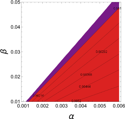
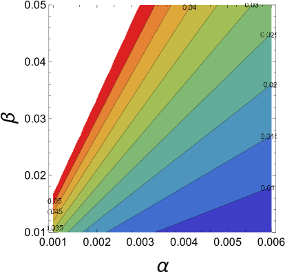
Figure 1: Contour plots for the spectral index of primordial scalar curvature perturbations $n_{s}$ (left plot) and the tensor-to-scalar ratio $r$ (right plot), for $\beta=[0.01,0.05]$, $\alpha=[0,0.006]$ and $N=60$.

Let us start our quantitative study of inflation for the rescaled Einstein-Hilbert gravity, by analyzing a supergravity $\alpha$-attractor model, for which the scalar potential is Carrasco:2015rva ,

$$V(\phi)=V_{0}^{4}\left(1-e^{-\sqrt{\frac{2}{3\beta}}\kappa\phi}\right)^{2}\,,$$ (26)

where $V_{0}$ is a constant with mass dimensions $[V_{0}]=m$ and $\beta$ is a dimensionless constant. The slow-roll index $\epsilon_{1}$ is easily found,

$$\epsilon_{1}=\frac{4\alpha}{3\beta\left(e^{\sqrt{\frac{2}{3}}\sqrt{\frac{1}{\beta}}\kappa\phi}-1\right)^{2}}\,,$$ (27)

and by solving the equation $\epsilon_{1}(\phi_{f})=1$, we obtain the value of the scalar field at the end of the inflationary era, which is,

$$\phi_{f}=\frac{\sqrt{\frac{3}{2}}\log\left(\frac{2\sqrt{3}\sqrt{\alpha}+3\sqrt{\beta}}{3\sqrt{\beta}}\right)}{\sqrt{\frac{1}{\beta}}\kappa}\,.$$ (28)

Accordingly, by integrating (23), we obtain the value of the scalar field at first horizon crossing,

$$\phi_{i}=\frac{\sqrt{\frac{3}{2}}\log\left(\frac{2\sqrt{3}\sqrt{\alpha}\sqrt{\beta}+3\beta+4\alpha N}{3\beta}\right)}{\sqrt{\frac{1}{\beta}}\kappa}\,.$$ (29)

Hence, the spectral index of the primordial scalar curvature perturbations, and the tensor-to-scalar ratio can be evaluated at leading order in $1/N$, and these are,

$$n_{s}\simeq 1-\frac{2}{N}+\frac{\sqrt{3}\sqrt{\beta}}{\sqrt{\alpha}N^{2}}-\frac{3\beta}{\alpha N^{2}}\,,$$ (30)

$$r\simeq\frac{12\beta}{\alpha N^{2}}\,.$$ (31)

The phenomenological viability of the model can be achieved for a large range of the free parameters $\alpha$ and $\beta$, for $N\sim 60$, however we shall choose both $\alpha$ and $\beta$ in such a way so both the inflationary phenomenology viability and the compliance with the Swampland conjectures is simultaneously achieved. In Fig. 1 we present the contour plots for the spectral index of primordial scalar curvature perturbations values (left plot) and the tensor-to-scalar ratio (right plot), for $\beta=[0.01,0.05]$ and $\alpha=[0,0.006]$ and $N=60$. Recall that the latest Planck constraints indicate that Akrami:2018odb ,

$$n_{s}=0.9649\pm 0.0042,\,\,\,r<0.056\,,$$ (32)

so in both the plots of Fig. 1, we kept values in the plot range that satisfy the latest Planck constraints, that is $n_{s}=[0.9607,0.9691]$ and $r=[0,0.056]$. As it can be seen, the simultaneous compatibility of both the spectral index $n_{s}$ and of the tensor-to-scalar ratio $r$ is achieved for this range of values of $\alpha$ and $\beta$. A numerical example would also be useful here, so for $\alpha=0.004$ and $\beta=0.02$ and for $N=60$, we get $n_{s}=0.963576$ and $r=0.0166667$, which are of course compatible with the latest Planck data (32). Now let us turn our focus on the Swampland criteria, and in Fig. 2 we plotted the contour plots of $\frac{V^{\prime}(\phi)}{V(\phi)}$ (left plot) and of $-\frac{V^{\prime\prime}(\phi)}{V(\phi)}$ (right plot), evaluated at the first horizon crossing (which is the relevant value of the scalar field for inflationary phenomenology) for the same range of values of the free parameters $\alpha$ and $\beta$, that is for, $\beta=[0.01,0.05]$ and $\alpha=[0,0.006]$ and for $N=60$, in reduced Planck units. In the left plot we kept the plot values of $\frac{V^{\prime}(\phi)}{V(\phi)}$ to be in the range $\frac{V^{\prime}(\phi)}{V(\phi)}=[1,9]$ while for $\frac{V^{\prime\prime}(\phi)}{V(\phi)}=[1,13]$, so both the quantities $\frac{V^{\prime}(\phi)}{V(\phi)}$ and of $-\frac{V^{\prime\prime}(\phi)}{V(\phi)}$ take values well above unity in reduced Planck units.

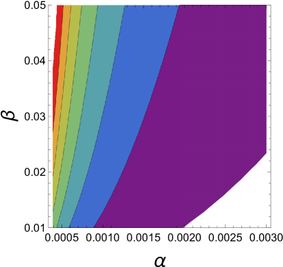
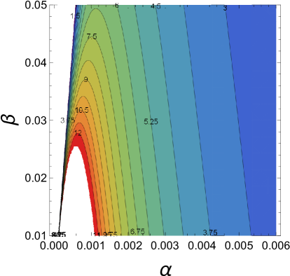
Figure 2: Second and third Swampland criteria analysis. Contour plots of $\frac{V^{\prime}(\phi)}{V(\phi)}$ (left plot) and of $-\frac{V^{\prime\prime}(\phi)}{V(\phi)}$ (right plot), evaluated at the first horizon crossing for the ranges of values of the free parameters, $\beta=[0.01,0.05]$ and $\alpha=[0,0.006]$ and for $N=60$, in reduced Planck units.

Hence, for the $\alpha$-attractor $E$-model, the last two Swampland criteria are satisfied. Finally, let us note that for all the analysis performed above, we assumed that the first Swampland criterion marginally holds true, so during inflation, the scalar field takes values $\Delta\phi\sim M_{p}$, or $\Delta\phi\sim 1$ in reduced Planck units.

IV Inflationary Phenomenology and Swampland Criteria for a Fibre Inflation Model

Let us now consider another model of phenomenological interest, which is related to several string theory models Stewart:1994ts ; Cicoli:2008gp , and is known as a class of fibre inflation, in which case the potential is,

$$V(\phi)=V_{0}^{4}(1-\exp(-\lambda\kappa\phi))\,,$$ (33)

where again the constant $V_{0}$ has mass dimensions $[V_{0}]=[m]$ and $\lambda$ is a dimensionless constant. In this case the slow-roll index $\epsilon_{1}$ is,

$$\epsilon_{1}=\frac{\alpha\lambda^{2}e^{-2\kappa\lambda\phi}}{2\left(1-e^{-\kappa\lambda\phi}\right)^{2}}\,,$$ (34)

and again by solving the equation $\epsilon_{1}(\phi_{f})=1$, we obtain $\phi_{f}$,

$$\phi_{f}=\frac{\log\left(\frac{1}{2}\left(2-\sqrt{2}\sqrt{\alpha}\lambda\right)\right)}{\kappa\lambda}\,.$$ (35)

Accordingly, by integrating (23), we get $\phi_{i}$,

$$\phi_{i}=\frac{\log\left(\frac{1}{2}\left(\sqrt{2}\sqrt{\alpha}\lambda+2\alpha\lambda^{2}N+2\right)\right)}{\kappa\lambda}\,.$$ (36)

Hence, the spectral index of the primordial scalar curvature perturbations, and the tensor-to-scalar ratio at leading order in $1/N$ are,

$$n_{s}\simeq 1-\frac{2}{N}-\frac{3}{\alpha\lambda^{2}N^{2}}+\frac{\sqrt{2}}{\sqrt{\alpha}\lambda N^{2}}\,,$$ (37)

$$r\simeq\frac{8}{\alpha\lambda^{2}N^{2}}\,.$$ (38)

In this case too, the model has good inflationary phenomenological properties, and the viability can be achieved for a large range of the free parameters $\alpha$ and $\lambda$, for $N\sim 60$. However, as in the previous paradigm, we shall choose $\alpha$ and $\lambda$ in such a way so that both the Swampland criteria are satisfied and the inflationary phenomenology of the model is guaranteed.

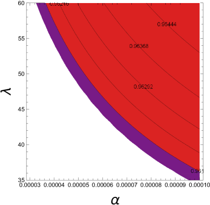
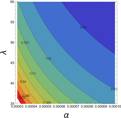
Figure 3: Contour plots for the spectral index of primordial scalar curvature perturbations $n_{s}$ (left plot) and the tensor-to-scalar ratio $r$ (right plot), for $\lambda=[35,60]$ and $\alpha=[0.00003,0.0001]$ and for $N=60$.

In Fig. 3 we present the contour plots for the spectral index of primordial scalar curvature perturbations values (left plot) and the tensor-to-scalar ratio (right plot), for $\lambda=[35,60]$ and $\alpha=[0.00003,0.0001]$ and $N=60$, and in both the plots of Fig. 3, we kept values in the plot range that satisfy the latest Planck constraints, that is $n_{s}=[0.9607,0.9691]$ and $r=[0,0.056]$. As it can be seen, for this model too, the simultaneous compatibility of both the spectral index $n_{s}$ and of the tensor-to-scalar ratio $r$ is achieved. Now let us turn our focus on the Swampland criteria, and in Fig. 4 we present the results of our numerical analysis. Particularly, the left contour plot corresponds to the values of $\frac{V^{\prime}(\phi)}{V(\phi)}$, and also the right contour plots corresponds to the values of $-\frac{V^{\prime\prime}(\phi)}{V(\phi)}$, evaluated at the first horizon crossing for $\lambda=[35,60]$ and $\alpha=[0.00003,0.0001]$ and $N=60$. In the left plot we kept the plot values of $\frac{V^{\prime}(\phi)}{V(\phi)}$ in the range $\frac{V^{\prime}(\phi)}{V(\phi)}=[1,9]$ while for $\frac{V^{\prime\prime}(\phi)}{V(\phi)}=[100,500]$, so both the quantities $\frac{V^{\prime}(\phi)}{V(\phi)}$ and of $-\frac{V^{\prime\prime}(\phi)}{V(\phi)}$ take values well above unity in reduced Planck units, especially $-\frac{V^{\prime\prime}(\phi)}{V(\phi)}$ takes quite large values for the same set of free parameters values .

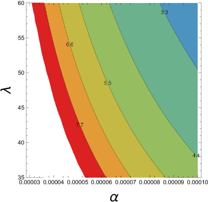
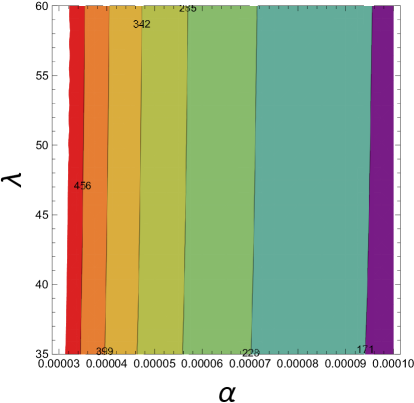
Figure 4: Second and third Swampland criteria analysis for the Fibre inflation model. Contour plots of $\frac{V^{\prime}(\phi)}{V(\phi)}$ (left plot) and of $-\frac{V^{\prime\prime}(\phi)}{V(\phi)}$ (right plot), evaluated at the first horizon crossing for the ranges of values of the free parameters $\alpha$ and $\lambda$, $\lambda=[35,60]$ and $\alpha=[0.00003,0.0001]$ and for $N=60$, in reduced Planck units.

Hence, in this case too, the last two Swampland criteria are satisfied and also we assumed that $\Delta\phi\sim M_{p}$, or $\Delta\phi\sim 1$ in reduced Planck units for the whole analysis.

IV.1 Dark Energy Evolution for the $f(R)$ Gravity Model with Fibre Inflation Potential

The motivation for studying the exponential $f(R)$ gravity models, was mainly the interesting late-time phenomenology these generate, as is the case in Ref. Oikonomou:2020qah , where the unification of inflation with the late-time era was obtained. In this work, we shall also consider the late-time phenomenology of the model (1) with the $f(R)$ gravity model being that of Eq. (2) and the scalar potential of the fibre inflation, namely that of Eq. (33), in the presence of cold dark matter and of radiation perfect fluids. The model of this work and the one studied in Ref. Oikonomou:2020qah are different in their functional form, but have similarities, however, in the present paper the inflationary era is controlled by a canonical scalar field, while in the model of Ref. Oikonomou:2020qah , the early-time era was controlled by an $R^{2}$ term, and the axion scalar was frozen in its primordial vacuum expectation value. Let us now study the late-time behavior of the $f(R)$ gravity canonical scalar field theory. To this end, instead of the cosmic time we shall express all the dynamically evolving quantities as functions of the redshift,

$$\centering 1+z=\frac{1}{a(t)}\,,\@add@centering$$ (39)

and also we shall make extensive use of the following differentiation rule,

$$\centering\frac{d}{dt}=-H(1+z)\frac{d}{dz}\,.\@add@centering$$ (40)

More importantly, we shall express all the Hubble rate dependent terms and their derivatives, as functions of the statefinder function $y_{H}(z)$ and its derivatives Hu:2007nk ; Bamba:2012qi ; Odintsov:2020qyw ; Odintsov:2020nwm ,

$$\centering y_{H}=\frac{\rho_{DE}}{\rho_{m}^{(0)}}\,,\@add@centering$$ (41)

with $\rho_{DE}$ standing for the dark matter energy density and with $\rho_{m}^{(0)}$ being the current value of density for non-relativistic matter. The forms of the dark energy density and of the dark energy pressure can be derived by the field equations corresponding to the action (1),

$$\centering\rho_{DE}=\frac{1}{2}\dot{\phi}^{2}+V+\frac{f_{R}R-f}{2\kappa^{2}}-\frac{3H\dot{f}_{R}}{\kappa^{2}}+\frac{3H^{2}}{\kappa^{2}}(1-f_{R})\,,\@add@centering$$ (42)

$$\centering P_{DE}=-V-\frac{f_{R}R-f}{2\kappa^{2}}-\frac{2\dot{H}}{\kappa^{2}}(1-f_{R})\,.\@add@centering$$ (43)

The field equations can be cast in their Einstein-Hilbert form for a FRW metric,

$$\centering\frac{3H^{2}}{\kappa^{2}}=\rho_{(m)}+\rho_{DE}\,,\@add@centering$$ (44)

$$\centering-\frac{2\dot{H}}{\kappa^{2}}=\rho_{(m)}+P_{(m)}+\rho_{DE}+P_{DE}\,,\@add@centering$$ (45)

where $\rho_{(m)}$ and $P_{(m)}$ are the energy density and the pressure of the matter perfect fluids that are present, which we shall assume that these are the radiation and cold-dark-matter fluids. Hence, the Hubble rate can be written as a function of the statefinder as follows,

$$\centering H^{2}=m_{s}^{2}\left(y_{H}(z)+\frac{\rho_{(m)}}{\rho_{m}^{(0)}}\right)\,,\@add@centering$$ (46)

where $m_{s}^{2}=\kappa^{2}\frac{\rho_{m}^{(0)}}{3}=1.87101\cdot 10^{-67}$eV². We shall solve numerically the field equations in the redshift interval $z=[0,10]$, by assuming the following initial conditions,

$$y_{H}(z_{f})=\frac{\Lambda}{3m_{s}^{2}}\left(1+\frac{(1+z_{f})}{1000}\right)\,,\,\,\,\frac{dy_{H}(z)}{dz}\Big{|}_{z=z_{f}}=\frac{1}{1000}\frac{\Lambda}{3m_{s}^{2}}\,,$$ (47)

for the function $y_{H}(z)$, where $z_{f}=10$, while for the scalar field, the initial conditions are chosen as,

$$\phi(z_{f})=10^{-16}M_{p},\,\,\,\phi^{\prime}(z_{f})=-10^{-7}M_{p}\,.$$ (48)

As for the free parameters and the various physical parameters, we shall assume that the Hubble rate at present time is $H_{0}\simeq 1.37187\times 10^{-33}$eV according to the latest Planck data Aghanim:2018eyx . In addition, $\Omega_{\Lambda}\simeq 0.681369$ and $\Omega_{M}\sim 0.3153$ Aghanim:2018eyx , while $\Omega_{r}/\Omega_{M}\simeq\chi$. Also for the numerical analysis of the model (2), we shall choose $\gamma=6$, $\zeta=0.23$ $\delta=0.01$ and $\lambda=0.001$. In addition, $m_{s}^{2}=\frac{\kappa^{2}\rho^{(0)}_{m}}{3}=H_{0}\Omega_{c}=1.37201\times 10^{-67}$eV², and $\Lambda$ is assumed to be equal to the present time cosmological constant, while $V_{0}$ appearing in Eq. (33) is chosen to be $V_{0}=\Lambda^{4}$. In Fig. 5 we present the statefinder $y_{H}(z)$ as a function of the redshift (left plot) and the dark energy EoS parameter as a function of the redshift (right plot).

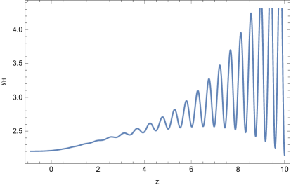
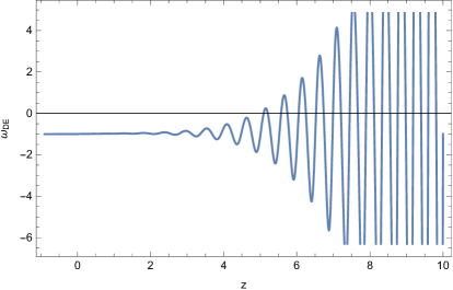
Figure 5: The statefinder function $y_{H}$ for geometric dark energy as a function of the redshift (left plot), and the dark energy EoS parameter $\omega_{DE}$ (right plot).

It is apparent that the dark energy oscillations are present even in this scalar $f(R)$ gravity model, while in the model of Ref. Oikonomou:2020qah , dark energy oscillations were absent. Hence it seems that the dark energy oscillations seem to be a model dependent feature of modified gravity models. In order to have a concrete quantitative idea of how viable is the model under study, let us calculate the dark energy equation of state (EoS) parameter $\omega_{DE}$, and the dark energy density parameter $\Omega_{DE}$ at present time, for the model under study. In terms of $y_{H}$, the aforementioned quantities are defined as Bamba:2012qi ; Odintsov:2020qyw ; Odintsov:2020nwm ,

$$\centering\omega_{DE}\@add@centering =-1+\frac{1+z}{3}\frac{d\ln{y_{H}}}{dz} \Omega_{DE} =\frac{y_{H}}{y_{H}+\frac{\rho_{(m)}}{\rho_{m}^{(0)}}}\,,$$ (49)

so our numerical analysis yielded the following values,

$$\centering\omega_{DE}(0)=-0.996093,\,\,\,\Omega_{DE}(0)=0.688719\,,\@add@centering$$ (50)

which are compatible with the latest Planck constraints on the cosmological parameters Aghanim:2018eyx , which indicate that $\omega_{DE}=-1.018\pm 0.031$, and $\Omega_{DE}=0.6847\pm 0.0073$. Finally, it is worth to compare in brief the present model with the $\Lambda$CDM model, so let us consider a statefinder quantity in order to reveal the resemblance of the $\Lambda$CDM model with the fibre $f(R)$ gravity model. We shall consider the deceleration parameter,

$$q=-1-\frac{\dot{H}}{H^{2}}=-1+(z+1)\frac{H^{\prime}(z)}{H(z)}\,,$$ (51)

and in Fig. 6 we present the deceleration parameter for the fibre $f(R)$ model (blue curve), with the $\Lambda$CDM deceleration parameter (red curve). As it can be seen in Fig. 6 the two models are indistinguishable for $z<4$. Also at present day, the deceleration parameter for the fibre $f(R)$ gravity model is $q(0)=-0.528993$, while the $\Lambda$CDM value is $q=-0.527$, which are quite similar values.

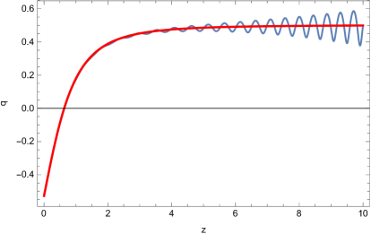
Figure 6: The deceleration parameter, as a function of the redshift for the fibre $f(R)$ gravity model (blue curve) and for the $\Lambda$CDM model (red curve).

Finally, our numerical analysis indicated that the initial condition of the scalar field at $z=z_{f}$ does not affect significantly the late-time qualitative behavior, however, the initial condition of the derivative of the scalar field with respect to the redshift variable, affects significantly the late-time behavior.

In conclusion, we demonstrated that the $f(R)$ gravity scalar field model with fibre inflation potential, can describe in an unified way both the inflationary era and the dark energy era, producing results which are both compatible with the 2018 Planck constraints on inflation Akrami:2018odb and with the 2018 Planck constraints on the cosmological parameters Aghanim:2018eyx . At the same time the model formally satisfies the Swampland criteria, for the same set of values of the free parameters that yield the inflationary viability of the model. The new result that the fibre $f(R)$ gravity model brings along is that the early-time era is essentially governed by a rescaled Einstein-Hilbert canonical scalar theory, and the rest of the $f(R)$ terms affect only the late-time era. The presence of a rescaled Ricci scalar term is a solid effect of modified gravity, which affects the inflationary effective Lagrangian at large curvatures.

Finally it is worthy discussing which term affects the most the dark energy era, is it the $f(R)$ gravity or the scalar field. The answer to this question can be given only qualitatively, and it seems that only $f(R)$ gravity drives the late-time era. The only effect of the scalar field is that it mainly affects the dark energy oscillations, which, in the absence of the scalar field and for the class of $f(R)$ models studied in this paper, are absent, see for example Ref. Oikonomou:2020qah . Also the viability of the model is obtained for different values of the exponent of the power-law $f(R)$ gravity term. Thus the scalar model changes the behavior of the dark energy era in a qualitative way since it changes the parameter range for which viability can occur, and also it re-introduces oscillations in the class of models studied in the present paper, which were absent in the scalar field free theory of Ref. Oikonomou:2020qah .

V Conclusions

In this work we presented a model of $f(R)$ gravity in the presence of a canonical scalar field, and we investigated a unification of inflation with dark energy scenario. The $f(R)$ gravity was chosen to be of exponential type with power-law corrections with their exponent being less than unity and positive. During the large curvature era, the $f(R)$ gravity at leading order became a rescaled type of Einstein-Hilbert gravity, with the dominant term being of the form $\alpha R$, with $\alpha$ being a dimensionless constant. Thus the effective Lagrangian during the inflationary era was that of a rescaled Einstein-Hilbert canonical scalar theory. For the inflationary era we investigated the phenomenologically viability of the resulting theory and also we examined whether it was possible to comply with the Swampland criteria. As we showed, this is possible for the resulting theory, if the first Swampland criterion holds marginally true, that is, if the scalar field during the inflationary era is of the order $\phi\sim M_{p}$. We exemplified our study by using two characteristic inflationary potentials, one supergravity related $\alpha$-attractors model, and one fibre inflation model. After examining carefully the parameter space of the two models, we showed that the phenomenologically viability of the models is easy to achieve, and also we demonstrated that for the same set of values for the free parameters that guarantee the inflationary viability of the models, the models became compatible with the Swampland criteria. Finally, we addressed the question whether it is possible to describe the inflationary and the dark energy era within this theoretical framework of $f(R)$ canonical scalar theory. By investigating the fibre inflationary potential at late times, using a numerical approach, we demonstrated that the $f(R)$ scalar theory can produce a viable dark energy, which is compatible with the latest 2018 Planck data and mimics the $\Lambda$CDM model, when statefinder quantities are considered. A notable feature characterizing the dark energy era, is the presence of dark energy oscillations, and by taking into account the results of Ref. Oikonomou:2020qah , we may reach the conclusion that the dark energy oscillations feature is a model depended feature in modified gravity dark energy models.

References

- (1) Y. Akrami et al. [Planck Collaboration], arXiv:1807.06211 [astro-ph.CO].
- (2) M. Denissenya and E. V. Linder, JCAP 11 (2018), 010 doi:10.1088/1475-7516/2018/11/010 [arXiv:1808.00013 [astro-ph.CO]].
- (3) A. G. Riess et al. [Supernova Search Team], Astron. J. 116 (1998) 1009 [astro-ph/9805201].
- (4) S. D. Odintsov, V. K. Oikonomou, F. P. Fronimos and K. V. Fasoulakos, Phys. Rev. D 102 (2020) no.10, 104042 doi:10.1103/PhysRevD.102.104042 [arXiv:2010.13580 [gr-qc]].
- (5) R. H. Brandenberger, arXiv:1206.4196 [astro-ph.CO].
- (6) R. Brandenberger and P. Peter, arXiv:1603.05834 [hep-th].
- (7) D. Battefeld and P. Peter, Phys. Rept. 571 (2015) 1 [arXiv:1406.2790 [astro-ph.CO]].
- (8) M. Novello and S. E. P. Bergliaffa, Phys. Rept. 463 (2008) 127 [arXiv:0802.1634 [astro-ph]].
- (9) Y. F. Cai, Sci. China Phys. Mech. Astron. 57 (2014) 1414 doi:10.1007/s11433-014-5512-3 [arXiv:1405.1369 [hep-th]].
- (10) J. de Haro and Y. F. Cai, Gen. Rel. Grav. 47 (2015) no.8, 95 [arXiv:1502.03230 [gr-qc]].
- (11) J. L. Lehners, Class. Quant. Grav. 28 (2011) 204004 [arXiv:1106.0172 [hep-th]].
- (12) J. L. Lehners, Phys. Rept. 465 (2008) 223 [arXiv:0806.1245 [astro-ph]].
- (13) Y. K. E. Cheung, C. Li and J. D. Vergados, arXiv:1611.04027 [astro-ph.CO].
- (14) Y. F. Cai, A. Marciano, D. G. Wang and E. Wilson-Ewing, Universe 3 (2016) no.1, 1 doi:10.3390/universe3010001 [arXiv:1610.00938 [astro-ph.CO]].
- (15) A. D. Linde, Lect. Notes Phys. 738 (2008) 1 doi:10.1007/978-3-540-74353-8_1 [arXiv:0705.0164 [hep-th]].
- (16) D. S. Gorbunov and V. A. Rubakov,“Introduction to the theory of the early universe: Cosmological perturbations and inflationary theory,” Hackensack, USA: World Scientific (2011) 489 p
- (17) D. H. Lyth and A. Riotto, Phys. Rept. 314 (1999) 1 doi:10.1016/S0370-1573(98)00128-8 [hep-ph/9807278].
- (18) J. Martin, arXiv:1807.11075 [astro-ph.CO].
- (19) S. Nojiri, S. D. Odintsov and V. K. Oikonomou, Phys. Rept. 692 (2017) 1 doi:10.1016/j.physrep.2017.06.001 [arXiv:1705.11098 [gr-qc]].
- (20) S. Nojiri, S.D. Odintsov, Phys. Rept. 505, 59 (2011);
- (21) S. Nojiri, S.D. Odintsov, eConf C0602061, 06 (2006) [Int. J. Geom. Meth. Mod. Phys. 4, 115 (2007)]. [arXiv:hep-th/0601213];
- (22) S. Capozziello, M. De Laurentis, Phys. Rept. 509, 167 (2011) [arXiv:1108.6266 [gr-qc]]. V. Faraoni and S. Capozziello, Fundam. Theor. Phys. 170 (2010). doi:10.1007/978-94-007-0165-6
- (23) A. de la Cruz-Dombriz and D. Saez-Gomez, Entropy 14 (2012) 1717 doi:10.3390/e14091717 [arXiv:1207.2663 [gr-qc]].
- (24) G. J. Olmo, Int. J. Mod. Phys. D 20 (2011) 413 doi:10.1142/S0218271811018925 [arXiv:1101.3864 [gr-qc]].
- (25) S. Nojiri and S. D. Odintsov, Phys. Rev. D 68 (2003) 123512 doi:10.1103/PhysRevD.68.123512 [hep-th/0307288].
- (26) S. Nojiri and S. D. Odintsov, Phys. Lett. B 657 (2007) 238 doi:10.1016/j.physletb.2007.10.027 [arXiv:0707.1941 [hep-th]].
- (27) S. Nojiri and S. D. Odintsov, Phys. Rev. D 77 (2008) 026007 doi:10.1103/PhysRevD.77.026007 [arXiv:0710.1738 [hep-th]].
- (28) G. Cognola, E. Elizalde, S. Nojiri, S. D. Odintsov, L. Sebastiani and S. Zerbini, Phys. Rev. D 77 (2008) 046009 doi:10.1103/PhysRevD.77.046009 [arXiv:0712.4017 [hep-th]].
- (29) S. Nojiri and S. D. Odintsov, Phys. Rev. D 74 (2006) 086005 doi:10.1103/PhysRevD.74.086005 [hep-th/0608008].
- (30) S. A. Appleby and R. A. Battye, Phys. Lett. B 654 (2007) 7 doi:10.1016/j.physletb.2007.08.037 [arXiv:0705.3199 [astro-ph]].
- (31) E. Elizalde, S. Nojiri, S. D. Odintsov, L. Sebastiani and S. Zerbini, Phys. Rev. D 83 (2011) 086006 doi:10.1103/PhysRevD.83.086006 [arXiv:1012.2280 [hep-th]].
- (32) S. D. Odintsov and V. K. Oikonomou, arXiv:2001.06830 [gr-qc].
- (33) V. K. Oikonomou, Phys. Rev. D 103 (2021) no.4, 044036 doi:10.1103/PhysRevD.103.044036 [arXiv:2012.00586 [astro-ph.CO]].
- (34) C. Vafa, hep-th/0509212.
- (35) H. Ooguri and C. Vafa, Nucl. Phys. B 766 (2007) 21 doi:10.1016/j.nuclphysb.2006.10.033 [hep-th/0605264].
- (36) E. Palti, C. Vafa and T. Weigand, arXiv:2003.10452 [hep-th].
- (37) S. Mizuno, S. Mukohyama, S. Pi and Y. L. Zhang, Phys. Rev. D 102 (2020) no.2, 021301 doi:10.1103/PhysRevD.102.021301 [arXiv:1910.02979 [astro-ph.CO]].
- (38) R. Brandenberger, V. Kamali and R. O. Ramos, arXiv:2002.04925 [hep-th].
- (39) R. Blumenhagen, M. Brinkmann and A. Makridou, JHEP 2002 (2020) 064 [JHEP 2020 (2020) 064] doi:10.1007/JHEP02(2020)064 [arXiv:1910.10185 [hep-th]].
- (40) Z. Wang, R. Brandenberger and L. Heisenberg, arXiv:1907.08943 [hep-th].
- (41) M. Benetti, S. Capozziello and L. L. Graef, Phys. Rev. D 100 (2019) no.8, 084013 doi:10.1103/PhysRevD.100.084013 [arXiv:1905.05654 [gr-qc]].
- (42) E. Palti, Fortsch. Phys. 67 (2019) no.6, 1900037 doi:10.1002/prop.201900037 [arXiv:1903.06239 [hep-th]].
- (43) R. G. Cai, S. Khimphun, B. H. Lee, S. Sun, G. Tumurtushaa and Y. L. Zhang, Phys. Dark Univ. 26 (2019) 100387 doi:10.1016/j.dark.2019.100387 [arXiv:1812.11105 [hep-th]].
- (44) Y. Akrami, R. Kallosh, A. Linde and V. Vardanyan, Fortsch. Phys. 67 (2019) no.1-2, 1800075 doi:10.1002/prop.201800075 [arXiv:1808.09440 [hep-th]].
- (45) S. Mizuno, S. Mukohyama, S. Pi and Y. L. Zhang, JCAP 1909 (2019) no.09, 072 doi:10.1088/1475-7516/2019/09/072 [arXiv:1905.10950 [hep-th]].
- (46) V. Aragam, S. Paban and R. Rosati, arXiv:1905.07495 [hep-th].
- (47) S. Brahma and M. W. Hossain, Phys. Rev. D 100 (2019) no.8, 086017 doi:10.1103/PhysRevD.100.086017 [arXiv:1904.05810 [hep-th]].
- (48) U. Mukhopadhyay and D. Majumdar, Phys. Rev. D 100 (2019) no.2, 024006 doi:10.1103/PhysRevD.100.024006 [arXiv:1904.01455 [gr-qc]].
- (49) S. Brahma and M. W. Hossain, JHEP 1906 (2019) 070 doi:10.1007/JHEP06(2019)070 [arXiv:1902.11014 [hep-th]].
- (50) M. R. Haque and D. Maity, Phys. Rev. D 99 (2019) no.10, 103534 doi:10.1103/PhysRevD.99.103534 [arXiv:1902.09491 [hep-th]].
- (51) J. J. Heckman, C. Lawrie, L. Lin, J. Sakstein and G. Zoccarato, Fortsch. Phys. 67 (2019) no.11, 1900071 doi:10.1002/prop.201900071 [arXiv:1901.10489 [hep-th]].
- (52) B. S. Acharya, A. Maharana and F. Muia, JHEP 1903 (2019) 048 doi:10.1007/JHEP03(2019)048 [arXiv:1811.10633 [hep-th]].
- (53) E. Elizalde and M. Khurshudyan, Phys. Rev. D 99 (2019) no.10, 103533 doi:10.1103/PhysRevD.99.103533 [arXiv:1811.03861 [astro-ph.CO]].
- (54) D. Y. Cheong, S. M. Lee and S. C. Park, Phys. Lett. B 789 (2019) 336 doi:10.1016/j.physletb.2018.12.046 [arXiv:1811.03622 [hep-ph]].
- (55) J. J. Heckman, C. Lawrie, L. Lin and G. Zoccarato, Fortsch. Phys. 67 (2019) no.10, 1900057 doi:10.1002/prop.201900057 [arXiv:1811.01959 [hep-th]].
- (56) W. H. Kinney, S. Vagnozzi and L. Visinelli, Class. Quant. Grav. 36 (2019) no.11, 117001 doi:10.1088/1361-6382/ab1d87 [arXiv:1808.06424 [astro-ph.CO]].
- (57) S. K. Garg and C. Krishnan, JHEP 1911 (2019) 075 doi:10.1007/JHEP11(2019)075 [arXiv:1807.05193 [hep-th]].
- (58) C. M. Lin, Phys. Rev. D 99 (2019) no.2, 023519 doi:10.1103/PhysRevD.99.023519 [arXiv:1810.11992 [astro-ph.CO]].
- (59) S. C. Park, JCAP 1901 (2019) 053 doi:10.1088/1475-7516/2019/01/053 [arXiv:1810.11279 [hep-ph]].
- (60) Y. Olguin-Trejo, S. L. Parameswaran, G. Tasinato and I. Zavala, JCAP 1901 (2019) 031 doi:10.1088/1475-7516/2019/01/031 [arXiv:1810.08634 [hep-th]].
- (61) H. Fukuda, R. Saito, S. Shirai and M. Yamazaki, Phys. Rev. D 99 (2019) no.8, 083520 doi:10.1103/PhysRevD.99.083520 [arXiv:1810.06532 [hep-th]].
- (62) S. J. Wang, Phys. Rev. D 99 (2019) no.2, 023529 doi:10.1103/PhysRevD.99.023529 [arXiv:1810.06445 [hep-th]].
- (63) H. Ooguri, E. Palti, G. Shiu and C. Vafa, Phys. Lett. B 788 (2019) 180 doi:10.1016/j.physletb.2018.11.018 [arXiv:1810.05506 [hep-th]].
- (64) H. Matsui, F. Takahashi and M. Yamada, Phys. Lett. B 789 (2019) 387 doi:10.1016/j.physletb.2018.12.055 [arXiv:1809.07286 [astro-ph.CO]].
- (65) G. Obied, H. Ooguri, L. Spodyneiko and C. Vafa, arXiv:1806.08362 [hep-th].
- (66) P. Agrawal, G. Obied, P. J. Steinhardt and C. Vafa, Phys. Lett. B 784 (2018) 271 doi:10.1016/j.physletb.2018.07.040 [arXiv:1806.09718 [hep-th]].
- (67) H. Murayama, M. Yamazaki and T. T. Yanagida, JHEP 1812 (2018) 032 doi:10.1007/JHEP12(2018)032 [arXiv:1809.00478 [hep-th]].
- (68) M. C. David Marsh, Phys. Lett. B 789 (2019) 639 doi:10.1016/j.physletb.2018.11.001 [arXiv:1809.00726 [hep-th]].
- (69) S. D. Storm and R. J. Scherrer, Phys. Rev. D 102 (2020) no.6, 063519 doi:10.1103/PhysRevD.102.063519 [arXiv:2008.05465 [hep-th]].
- (70) O. Trivedi, [arXiv:2008.05474 [hep-th]].
- (71) U. K. Sharma, [arXiv:2005.03979 [physics.gen-ph]].
- (72) S. D. Odintsov and V. K. Oikonomou, Phys. Lett. B 805 (2020), 135437 doi:10.1016/j.physletb.2020.135437 [arXiv:2004.00479 [gr-qc]].
- (73) A. Mohammadi, T. Golanbari, J. Enayati, S. Jalalzadeh and K. Saaidi, [arXiv:2011.13957 [gr-qc]].
- (74) O. Trivedi, [arXiv:2011.14316 [astro-ph.CO]].
- (75) C. Han, S. Pi and M. Sasaki, Phys. Lett. B 791 (2019), 314-318 doi:10.1016/j.physletb.2019.02.037 [arXiv:1809.05507 [hep-ph]].
- (76) A. Achúcarro and G. A. Palma, JCAP 02 (2019), 041 doi:10.1088/1475-7516/2019/02/041 [arXiv:1807.04390 [hep-th]].
- (77) Y. Akrami, M. Sasaki, A. R. Solomon and V. Vardanyan, [arXiv:2008.13660 [astro-ph.CO]].
- (78) E. Ó Colgáin, M. H. P. M. van Putten and H. Yavartanoo, Phys. Lett. B 793 (2019), 126-129 doi:10.1016/j.physletb.2019.04.032 [arXiv:1807.07451 [hep-th]].
- (79) E. Ó. Colgáin and H. Yavartanoo, Phys. Lett. B 797 (2019), 134907 doi:10.1016/j.physletb.2019.134907 [arXiv:1905.02555 [astro-ph.CO]].
- (80) A. Banerjee, H. Cai, L. Heisenberg, E. Ó. Colgáin, M. M. Sheikh-Jabbari and T. Yang, [arXiv:2006.00244 [astro-ph.CO]].
- (81) E. D. Stewart, Phys. Rev. D 51 (1995), 6847-6853 doi:10.1103/PhysRevD.51.6847 [arXiv:hep-ph/9405389 [hep-ph]].
- (82) M. Cicoli, C. P. Burgess and F. Quevedo, JCAP 03 (2009), 013 doi:10.1088/1475-7516/2009/03/013 [arXiv:0808.0691 [hep-th]].
- (83) J. J. M. Carrasco, R. Kallosh and A. Linde, Phys. Rev. D 92 (2015) no.6, 063519 doi:10.1103/PhysRevD.92.063519 [arXiv:1506.00936 [hep-th]].
- (84) J. c. Hwang and H. Noh, Phys. Rev. D 71 (2005) 063536 doi:10.1103/PhysRevD.71.063536 [gr-qc/0412126].
- (85) W. Hu and I. Sawicki, Phys. Rev. D 76 (2007) 064004 [arXiv:0705.1158 [astro-ph]].
- (86) K. Bamba, A. Lopez-Revelles, R. Myrzakulov, S. D. Odintsov and L. Sebastiani, Class. Quant. Grav. 30 (2013) 015008 [arXiv:1207.1009 [gr-qc]].
- (87) S. D. Odintsov, V. K. Oikonomou and F. P. Fronimos, Phys. Dark Univ. 29 (2020), 100563 doi:10.1016/j.dark.2020.100563 [arXiv:2004.08884 [gr-qc]].
- (88) N. Aghanim et al. [Planck Collaboration], arXiv:1807.06209 [astro-ph.CO].