Hawking radiation from nonrotating singularity-free black holes in conformal gravity

Abstract

We study the sparsity of Hawking radiation from nonrotating singularity-free black holes in conformal gravity. We give a rigorous bound on the greybody factor for massless scalar field and calculate the sparsity of Hawking radiation from the black hole. Besides, we investigate the dependence of the bound of the greybody factor and the sparsity of Hawking radiation on the conformal parameters respectively. Our study shows that when the conformal parameters are large, the increase of conformal parameters will lead to a more sparse Hawking radiation, while to a less sparse Hawking radiation if the conformal parameters are small.

I Introduction

Einstein’s general relativity is the most elegant and successful gravitational theory subjected to current experimental tests. However, this theory is still imperfect. One of the most important problems of Einstein’s gravity is that singularity is inevitable in almost all of its solutions. Since the existence of the singularity in spacetime, causality will break down, and the predicability of the theory will be lost at this point thus to find the solution for the singularity problem becomes theoretically essential. There are many proposals devoted to solving this problem, one attempt is to construct modified gravitational theories which have the properties of conformal invariance Englert:1976ep ; narlikar:1977nf ; Fradkin:1978yw ; Kaku:1982xu ; tHooft:2009wdx ; Mannheim:2011ds ; Bars:2013yba ; Prester:2013fia . A gravity theory is conformal invariant if its action is invariant under following transformation of metric

$${g_{\mu\nu}}\to{g^{\prime}_{\mu\nu}}=S\left(x\right){g_{\mu\nu}},$$ (1)

where $S\left(x\right)$ is a regular conformal factor depending on spacetime coordinate. Obviously, Einstein’s gravity is not conformal invariant. There are several ways to construct a conformal invariant gravity theory, for example, by introducing an auxiliary field Dirac:1973gk or the conformal invariant Weyl curvature tensor in the action Mannheim:2011ds ; Mannheim:2016lnx .

Einstein’s gravity is invariant under coordinate transformation, and the singularity at the event horizon can be removed by coordinate transformation therefore this singularity is not intrinsic as to Einstein’s gravity. Similarly in the context of conformal gravity theory, since the singularity at $r=0$ can in principle be removed by suitable choice of conformal transformation, hence conformal gravity is free from the singularity. However, the universe we are living in is not conformal invariant, and if the conformal gravity theory can describe the real universe, then there must be a phase transition at which the conformal symmetry is spontaneously broken. In the broken phase, there are singular and regular metrics with different physical properties due to that the conformal symmetry no longer exists, and it was assumed that our nature has a kind of unknown mechanism to select among these different conformal invariant spacetimes Toshmatov:2017kmw . We believe conformal gravity theory is viable and actually, a class of non-singular black hole spacetime solutions from conformal gravity are compatible with the data from the X-ray observation Bambi:2017yoz ; Zhou:2018bxk .

In this paper, we will study the nonrotating singularity-free black hole which was found in Modesto:2016max ; Bambi:2016wdn . The formation and evaporation process of this black hole has been analyzed in Bambi:2016yne , the quasinormal modes of various kinds of perturbations such as scalar, electromagnetic, axial, and gravitational perturbations in this black hole have been studied in Toshmatov:2017bpx ; Chen:2019iuo ; Liu:2020ddo . Besides, the violation of energy condition for this black hole has been investigated in Toshmatov:2017kmw . However, the greybody factor of this black hole is barely explored. So far only the greybody factor of the massless scalar field from this black hole has been numerically studied in Lin:2020rvv recently. In this paper, we give a rigorous lower bound for the greybody factor of the massless scalar field radiated from the black hole and study the sparsity of the Hawking radiation. Additionally, we investigate the effects of the variation of conformal factor parameters $N$ and $L$ (see eq.(4)) on the greybody factor and the sparsity of the Hawking radiation.

The paper is organized as follows. In section.II, we briefly review the nonrotating singularity-free black hole solution obtained in Modesto:2016max ; Bambi:2016wdn and the Regge-Wheeler equation for massless scalar field from this black hole derived in Toshmatov:2017bpx . In section.III, we study the power spectrum of Hawking radiation and calculate the rigorous lower bound of the greybody factor for the massless scalar field. Moreover, we give the values for conformal parameters which maximize the lower bound on the greybody factor numerically. Various numerical results for the upper bound of dimensionless parameter $\eta$ used to measure the sparsity of Hawking radiation are given in section.IV. Finally, in section.V we summarize the results of this paper and give a discussion. The geometric units, $\hbar{\rm{=}}c={k_{\rm{B}}}=G=1$, are adopted in this paper.

II Non-singular black holes in conformal gravity

In this section, we briefly review the nonrotating singularity-free black hole solution in conformal gravity Modesto:2016max ; Bambi:2016wdn .

The construction of the black hole solution is straightforward and is obtained by simply rescaling the Schwarzschild metric with a conformal factor as follows

$$d{s^{2}}=S(r)ds_{Schw}^{2},$$ (2)

where $ds_{Schw}^{2}$ is the line element of Schwarzschild black hole

$$ds_{Schw}^{2}=-\left(1-\frac{r_{\text{H}}}{r}\right)d{t^{2}}+\frac{dr^{2}}{\left(1-\frac{r_{\text{H}}}{r}\right)}+{r^{2}}d{\Omega_{2}^{2}},$$ (3)

in which $r_{\text{H}}$ is the horizon radius and $S(r)$ is the conformal factor

$$S(r)={\left({1+\frac{{{L^{2}}}}{{{r^{2}}}}}\right)^{2N}},$$ (4)

and $N$ is an arbitrary positive integer and $L$ is a new length scale which can be either of the order of Planck scale or of the order of the mass $M$ of the black hole. Due to the metric is conformal to the Schwarzschild black hole, the Hawking temperature of the black hole is still $T={1}/{(4\pi r_{\text{H}})}$. This metric can be the solution of a family of conformally invariant theories, since usually solutions of Einstein’s gravity theory are a subset of the wider class solutions of conformally invariant theories Grumiller:2013mxa ; Sultana:2012qp ; Said:2014lua , and indeed, metric in eq.(2) is obtained by the conformal transformation of Schwarzschild metric. It can be verified that the square of the Riemann tensor ${R_{\alpha\beta\gamma\delta}}{R^{\alpha\beta\gamma\delta}}$ of this spacetime is regular everywhere including $r=0$. Besides the spacetime is geodesically complete in the sense that it will take infinite proper time for a particle to reach $r=0$ (for more details see Ref.Bambi:2016wdn ).

The Klein-Gordon equation for a massless scalar field is

$$\frac{1}{{\sqrt{-g}}}{\partial_{\mu}}({g^{\mu\nu}}\sqrt{-g}{\partial_{\nu}}\Phi)=0.$$ (5)

Decomposing $\Phi{\rm{=}}{e^{-i\omega t}}\frac{{\psi\left(r\right)}}{{r\sqrt{S(r)}}}Y_{m}^{\ell}(\theta,\phi)$ and using the tortoise coordinate $d{r_{*}}=\frac{{dr}}{{f(r)}}$, the resulting Regge-Wheeler equation is Toshmatov:2017bpx

$$\left({\frac{{{d^{2}}}}{{d{r_{*}}^{2}}}+{\omega^{2}}-{V_{{\rm{eff}}}}}\right)\psi\left(r\right)=0,$$ (6)

where the effective potential ${{V_{{\rm{eff}}}}}$ is defined as

$${V_{{\rm{eff}}}}\equiv f(r)\left[{\frac{{\ell\left({\ell+1}\right)}}{{{r^{2}}}}+\frac{{\frac{d}{{dr}}\left({f(r)\frac{d}{{dr}}\left({r\sqrt{S(r)}}\right)}\right)}}{{r\sqrt{S(r)}}}}\right].$$ (7)

III Hawking radiation and Greybody factor

As discussed in Gray:2015pma ; Miao:2017jtr ; Chowdhury:2020bdi , the energy emitted per unit time for a 4-dimensional black hole is

$$\frac{{dE\left(\omega\right)}}{{dt}}=\sum\limits_{\ell}{{\Gamma_{\ell}}\left(\omega\right)}\frac{\omega}{{{e^{{\omega\mathord{\left/{\vphantom{\omega T}}\right.\kern-1.2pt}T}}}-1}}\hat{\vec{k}}\cdot\hat{\vec{n}}\frac{{{d^{3}}kdA}}{{{{\left({2\pi}\right)}^{3}}}},$$ (8)

where $dA$ is the infinitesimal surface area, $\hat{\vec{k}}$ is the unit tangent vector of the momentum of the scalar field, $\hat{\vec{n}}$ is the unit normal vector of $dA$, and ${{\Gamma_{\ell}}\left(\omega\right)}$ is the greybody factor. Since the scalar field we consider is massless thus $|{\vec{k}}|=\omega$, then the energy emitted per unite time on finite surface $A$ is

$$P=\sum\limits_{\ell}{\int{{P_{\ell}}\left(\omega\right)d\omega}}$$ (9)

with

$${P_{\ell}}\left(\omega\right)=\frac{A}{{8{\pi^{2}}}}\frac{{{\Gamma_{\ell}}\left(\omega\right){\omega^{3}}}}{{{e^{{\omega\mathord{\left/{\vphantom{\omega T}}\right.\kern-1.2pt}T}}}-1}}.$$ (10)

It was shown that $A$ can be taken as 27/4 times the horizon area for Schwarzschild black hole to match high frequency results Page:1976df ; Gray:2015pma , and here we can also take this value, since the cross section in geometrical optical limit for massless particle in this model is the same as that of Schwarzschild black hole Lin:2020rvv . Besides, the Hawking temperature $T$ is independent of conformal parameters $N$ and $L$ (see section.II). Therefore, the dependence of power spectrum ${P_{\ell}}\left(\omega\right)$ for Hawking radiation on conformal parameters $N$ and $L$ is as same as that of greybody factor ${\Gamma_{\ell}}\left(\omega\right)$.

Calculating the analytical expression for greybody factor is generally impractical and usually, it is obtained from numerical computations Harris:2004mf ; Harris:2005jx ; Kanti:2005ja ; Duffy:2005ns . The analytical calculations are available only in some special cases, such as the low frequency limit Unruh:1976fm ; Rocha:2009xy ; Harmark:2007jy ; Kanti:2014dxa ; Anderson:2015bza ; Sporea:2015hla , the near extremal limit Cvetic:2009jn ; Bredberg:2009pv ; Chen:2010bsa ; Chen:2010as ; Chen:2010ywa ; Chen:2010yu , or the large spacetime dimension limit Emparan:2013xia ; Emparan:2013moa ; Guo:2015swu ; Emparan:2020inr . In this paper, we follow Visser:1998ke ; Boonserm:2008zg ; Boonserm:2014rma to give a rigorous lower bound for the greybody factor. The bound for greybody factor can be written as follow

$${{\Gamma_{\ell}}\left(\omega\right)}\geqslant{\rm{sec}}{{\rm{h}}^{2}}\left\{{\int_{-\infty}^{\infty}{\vartheta d{r_{*}}}}\right\}$$ (11)

with

$$\vartheta=\frac{{\sqrt{{{\left({h^{\prime}\left(r\right)}\right)}^{2}}+{{\left({{\omega^{2}}-{V_{{\rm{eff}}}}-h{{\left(r\right)}^{2}}}\right)}^{2}}}}}{{2h\left(r\right)}},$$ (12)

where $h(r)$ is an arbitrary positive definite function and satisfy the limits $h(-\infty)=h(+\infty)=\omega$. A particularly simple choice of $h(r)$ is $h(r)=\omega$, which leads to

$$\int_{-\infty}^{\infty}{\vartheta d{r_{*}}}=\int_{2M}^{\infty}{\frac{{{V_{{\rm{eff}}}}}}{{2\omega f(r)}}dr}.$$ (13)

Combining eq.(7) and eq.(13) we have

$$\int_{-\infty}^{\infty}{\vartheta d{r_{*}}}=\frac{{2NM(2N-1)}}{{\omega{L^{2}}}}\ln\left({1+\frac{{{L^{2}}}}{{4{M^{2}}}}}\right)+\frac{{N\left({3N-2}\right)}}{{{\rm{2}}\omega L}}\left[{2\arctan\left({\frac{{2M}}{L}}\right)-\pi}\right]+\frac{{{{\left({2N-1}\right)}^{2}}}}{{8\omega M}}+\frac{{\ell\left({\ell+1}\right)}}{{4\omega M}},$$ (14)

where $M$ is the mass of the black hole. Substituting the above equation into eq.(11), we obtain the bound as

$${{\Gamma_{\ell}}\left(\omega\right)}\geqslant{\rm{sec}}{{\rm{h}}^{2}}\left\{{\frac{{2NM(2N-1)}}{{\omega{L^{2}}}}\ln\left({1+\frac{{{L^{2}}}}{{4{M^{2}}}}}\right)+\frac{{N\left({3N-2}\right)}}{{{\rm{2}}\omega L}}\left[{2\arctan\left({\frac{{2M}}{L}}\right)-\pi}\right]+\frac{{{{\left({2N-1}\right)}^{2}}}}{{8\omega M}}+\frac{{\ell\left({\ell+1}\right)}}{{4\omega M}}}\right\}.$$ (15)

Now let us analyze the dependence of this bound on the parameters $N$ and $L$ in various situations. At first, for $N=0$ we have

$${{\Gamma_{\ell}}\left(\omega\right)}\geqslant{\rm{sec}}{{\rm{h}}^{2}}\left\{{\frac{{\ell\left({\ell+1}\right)}}{{4\omega M}}+\frac{1}{{8\omega M}}}\right\},$$ (16)

which is exactly the result for Schwarzschild black hole as it should be. Note that this result has been obtained in Boonserm:2008zg . In addition, when $L$ is large, the bound in eq.(15) can be simplified as follows

$${{\Gamma_{\ell}}\left(\omega\right)}\geqslant{\text{sec}}{{\text{h}}^{2}}\left\{{\frac{{\ell\left({\ell+1}\right)}}{{4\omega M}}+\frac{{{{\left({2N-1}\right)}^{2}}}}{{8\omega M}}}\right\},$$ (17)

while in small $L$ limit eq.(15) reduces to eq.(16).

Furthermore, it is not hard to find out specific values for the conformal parameters $N$ and $L$ that can maximize the lower bound obtained in eq.(15). Specifically it can be done as follows. We first rewrite eq.(15) as

$${\Gamma_{\ell}}\left(\omega\right)\geqslant{\text{sec}}{{\text{h}}^{2}}\left\{{{{J\left({L,N,\ell}\right)}\mathord{\left/{\vphantom{{h\left({L,N,\ell}\right)}{\left({\omega{r_{\text{H}}}}\right)}}}\right.\kern-1.2pt}{\left({\omega{r_{\text{H}}}}\right)}}}\right\},$$ (18)

where we have defined

$$J\left({L,N,\ell}\right)\equiv\frac{{N(2N-1)}}{{{{\left({L/{r_{\text{H}}}}\right)}^{2}}}}\ln\left({1+\frac{{{L^{2}}}}{{r_{\text{H}}^{\text{2}}}}}\right)+\frac{{N\left({3N-2}\right)}}{{{\text{2}}\left({L/{r_{\text{H}}}}\right)}}\left[{2\arctan\left({\frac{{{r_{\text{H}}}}}{L}}\right)-\pi}\right]+\frac{{{{\left({2N-1}\right)}^{2}}}}{4}+\frac{{\ell\left({\ell+1}\right)}}{2}.$$ (19)

Note the function $y(x)={\operatorname{sech}^{2}}(x)$ is even, monotonously decreasing when $x>0$, and reaches its maximum at $x=0$, thus at fixed $\omega$, the values of $N$ and $L$ that minimize $\left|{J\left({L,N,\ell}\right)}\right|$ will maximize ${\text{sec}}{{\text{h}}^{2}}\left\{{{{J\left({L,N,\ell}\right)}\mathord{\left/{\vphantom{{h\left({L,N,\ell}\right)}{\left({\omega{r_{\text{H}}}}\right)}}}\right.\kern-1.2pt}{\left({\omega{r_{\text{H}}}}\right)}}}\right\}$. Therefore to obtain the values for $N$ and $L$ that can maximize the greybody factor we only need to find out the values that can minimize $\left|{J\left({L,N,\ell}\right)}\right|$.

In TABLE.1 and TABLE.2, for given values of ${L\mathord{\left/{\vphantom{L{{r_{\text{H}}}}}}\right.\kern-1.2pt}{{r_{\text{H}}}}}$($N$), we find out numerically the corresponding $N$(${L\mathord{\left/{\vphantom{L{{r_{\text{H}}}}}}\right.\kern-1.2pt}{{r_{\text{H}}}}}$) which can maximize the lower bound obtained in eq.(15).

Table 1: For different values of $L/r_{\text{H}}$ the corresponding values of $N$ which maximize the lower bound on greybody factor with $\ell=0$.

${L\mathord{\left/{\vphantom{L{{r_{\text{H}}}}}}\right.\kern-1.2pt}{{r_{\text{H}}}}}$	$0.1$	$0.3$	$0.5$	$0.7$	$0.9$	$1.5$	$2$	$2.5$	$3$
$N$	8	8	6	3	2	1	1	1	1

Table 2: For different values of $N$ the corresponding values of $L/{r_{\text{H}}}$ which maximize the lower bound on greybody factor with $\ell=0$.

$N$	$1$	$3$	$5$	$7$	$9$	$12$	$15$	$20$
${L\mathord{\left/{\vphantom{L{{r_{\text{H}}}}}}\right.\kern-1.2pt}{{r_{\text{H}}}}}$	2.893	0.785	0.558	0.456	0.395	0.337	0.299	0.257

To see the dependence of greybody factor and power spectrum of Hawking radiation on conformal parameters $N$, $L$, and the frequency $\omega$, intuitively, we plot the lower bound of greybody factor and power spectrum of Hawking radiation as a function of frequency for different values of $N$ and $L$. FIG.1 shows that, when the value of ${L\mathord{\left/{\vphantom{L{{r_{\rm{H}}}}}}\right.\kern-1.2pt}{{r_{\rm{H}}}}}$ is fixed, the increase of $N$ leads the lower bound of the greybody factor to increase at first (top left) and then to decrease (top right). Similarly the increase of ${L\mathord{\left/{\vphantom{L{{r_{\rm{H}}}}}}\right.\kern-1.2pt}{{r_{\rm{H}}}}}$ will enhance the lower bound of the greybody factor at the beginning (bottom left) and suppress it later (bottom right) for a given value of $N$. Obviously FIG.1 is consistent with TABLE.1 and TABLE.2.

Furthermore, as shown in FIG.2, for a fixed value of $L/{r_{\rm H}}$, the peak value of lower bound on the power spectrum of Hawking radiation increases as the increase of $N$ in the first place and decreases if $N$ continue to grow. While from the bottom of FIG.2 one can find that for a relatively small value of $L/{r_{\rm H}}$ the growth of $L/{r_{\rm H}}$ will cause the peak value of the lower bound on the Hawking radiation power spectrum to increase. Once $L/{r_{\rm H}}$ becomes relatively larger the increase of $L/{r_{\rm H}}$ will give rise to the decrease of the peak value of the lower bound of the power spectrum when $N$ is fixed. Also, we find that the values of $L/{r_{\rm H}}$ and $N$ which maximize the lower bound of the power spectrum of Hawking radiation are exactly those values for $L/{r_{\rm H}}$ and $N$ that maximize the lower bound of the greybody factor, which is in agreement with our analysis about the dependence of the lower bound on the Hawking radiation’s power spectrum on $N$ and $L$ above.

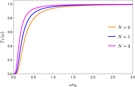
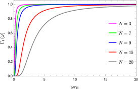
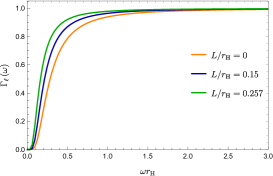
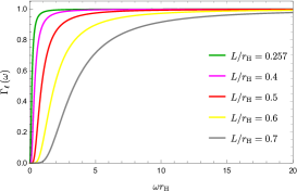
Figure 1: (Top) Plots of the lower bound of Greybody factor ${{\Gamma_{\ell}}\left(\omega\right)}$ as a function of $\omega r_{\text{H}}$ for different values of $N$ with $\ell=0$ and ${L}/{r_{\text{H}}}=0.7$; (Bottom) Plots of the bound of Greybody factor ${{\Gamma_{\ell}}\left(\omega\right)}$ as a function of $\omega r_{\text{H}}$ for different values of ${L}/{r_{\text{H}}}$ with $\ell=0$ and $N=20$.

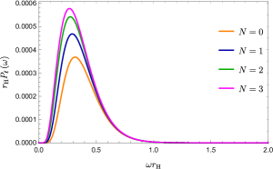
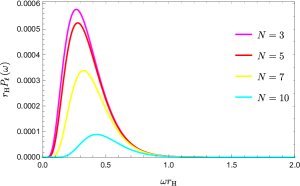
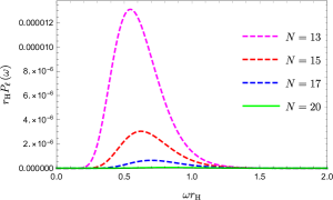
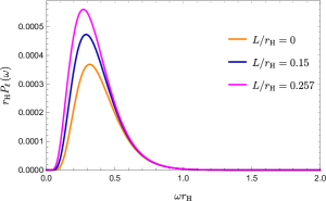
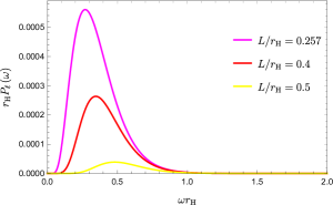
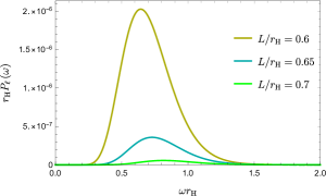
Figure 2: (Top) Plots of lower bounds on the power spectrum ${r_{\rm{H}}}{P_{\ell}}\left(\omega\right)$ as a function of $\omega r_{\text{H}}$ for different values of $N$ with $\ell=0$ and ${L}/{r_{\text{H}}}=0.7$; (Bottom) Plots of lower bounds on the power spectrum

${r_{\rm{H}}}{P_{\ell}}\left(\omega\right)$ as a function of $\omega r_{\text{H}}$ for different values of ${L}/{r_{\text{H}}}$ with $\ell=0$ and $N=20$.

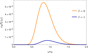
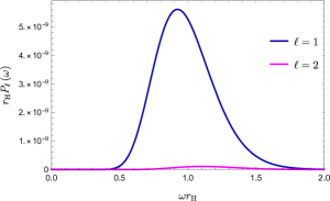
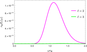
Figure 3: Plots of lower bounds on the power spectrum ${r_{\rm{H}}}{P_{\ell}}\left(\omega\right)$ as a function of $\omega r_{\text{H}}$ for different values of $\ell$ with $N=20$ and ${L}/{r_{\text{H}}}=0.7$.

IV The sparsity of Hawking radiation

The sparsity of Hawking radiation can be measured by the following quantity Gray:2015pma

$$\eta=\frac{{{\tau_{{\rm{gap}}}}}}{{{\tau_{{\rm{emission}}}}}},$$ (20)

where ${{\tau_{{\rm{gap}}}}}$ is the average time interval between the emission of two Hawking quanta, which is proportional to inverse of the total Hawking radiation power $P$ in eq.(9). More specifically, it can be computed by Gray:2015pma ; Paul:2016xvb

$${\tau_{{\rm{gap}}}}=\frac{{{\omega_{{\rm{peak}}}}}}{P},$$ (21)

here ${{\omega_{{\rm{peak}}}}}$ is the value at which the power spectrum $\sum\limits_{\ell}{{P_{\ell}}\left(\omega\right)}$ in eq.(9) is maximized. Before computing $\omega_{\text{peak}}$, let’s show a fact that in eq.(9), we can make an approximation that we only need to consider the term with $\ell=0$ in the summation. The justification of this approximation can be obtained by the observation of FIG.3 . Obviously, we can ignore the Hawking radiation modes with $\ell\neq 0$. So we can have

$$P\approx\int{{P_{\ell}}}\left(\omega\right)d\omega{\text{ }}\left({\ell=0}\right),$$ (22)

and naturally, we can choose the value that maximizes ${P_{\ell}}\left(\omega\right){\text{ }}\left({\ell=0}\right)$ (In what follows, we will simply express it as ${{P_{0}}\left(\omega\right)}$.) for $\omega_{\text{peak}}$. For different parameters $N$ and $L$, the values we found for ${{\omega_{{\text{peak}}}}}$ are shown in the TABLE.3 and TABLE.4.

Table 3: Numerical values of ${\omega_{{\text{peak}}}}{r_{H}}$ for different values of $N$ with $\ell=0$ and ${L}/{{{r_{\rm{H}}}}}=0.7$.

$N$	$0$	$1$	$2$	$3$	$4$	$5$	$6$	$7$	$8$	$9$	$10$	$15$	$20$
${\omega_{{\text{peak}}}}{r_{H}}$	0.316	0.291	0.275	0.267	0.268	0.279	0.297	0.324	0.356	0.391	0.428	0.623	0.817

Table 4: Numerical values of ${\omega_{{\text{peak}}}}{r_{H}}$ for different values of ${L}/{{{r_{\rm{H}}}}}$ with $\ell=0$ and $N=20$.

${L\mathord{\left/{\vphantom{L{{r_{\rm{H}}}}}}\right.\kern-1.2pt}{{r_{\rm{H}}}}}$	0	0.05	0.1	0.15	0.2	0.257	0.3	0.35	0.4	0.5	0.7
${\omega_{{\text{peak}}}}{r_{H}}$	0.316	0.312	0.303	0.290	0.278	0.271	0.276	0.301	0.346	0.482	0.817

Table 5: Numerical values of dimensionless parameter ${\eta_{\max}}$ for different values of $N$ with $\ell=0$ and ${L}/{{{r_{\rm{H}}}}}=0.7$.

$N$	$0$	$1$	$2$	$3$	$4$	$5$	$6$	$7$	$8$	$9$	$10$	$15$	$20$
${\eta_{\max}}$	122.8	83.0	63.9	56.6	57.7	67.8	$91.6$	$140.3$	$238.5$	$440.6$	$868.2$	$45850$	$3.85\times 10^{6}$

Table 6: Numerical values of dimensionless parameter ${\eta_{\max}}$ for different values of ${L}/{{{r_{\rm{H}}}}}$ with $\ell=0$ and $N=20$.

${L\mathord{\left/{\vphantom{L{{r_{\rm{H}}}}}}\right.\kern-1.2pt}{{r_{\rm{H}}}}}$	0	0.05	0.1	0.15	0.2	0.257	0.3	0.35	0.4	0.5	0.7
${\eta_{\max}}$	122.8	116.4	100.3	81.5	66.7	59.9	65.6	96.4	202.9	2407.02	$3.85\times 10^{6}$

${{\tau_{{\rm{emission}}}}}$ is the characteristic time for an individual quantum emitted from black hole, which can be taken equal to the period of the quantum emitted, since the quanta emitted at peak value can only be temporarily localized within a few oscillation periods. Therefore $\tau_{{\text{emission}}}$ obeys the bound

$${\tau_{{\text{emission}}}}\geqslant\frac{{2\pi}}{{{\omega_{{\text{peak}}}}}},$$ (23)

which leads to an upper bound for sparsity

$${\eta\leqslant\frac{{\omega_{{\text{peak}}}^{2}}}{{2\pi P}}\equiv{\eta_{\max}}\approx\frac{{\omega_{{\text{peak}}}^{2}}}{{2\pi\int{{P_{0}}\left(\omega\right)d\omega}}}.}$$ (24)

Since the exact value for greybody factor is unknown so far, we will use its lower bound in (15) to calculate ${P_{0}}\left(\omega\right)$ in (24), and we have given our corresponding argument in the footnote (3).

In summary, the sparsity of radiation in eq.(20) tells us that if $\eta\gg 1$, i.e. the average interval time $\tau_{{\rm{gap}}}$ between the emission of two quanta is much larger than the time $\tau_{{\text{emission}}}$ taken by an individual quantum emitted from the black hole, then naturally the Hawking radiation would be very sparse. On the contrary, if $\eta\ll 1$ we will have almost continuous Hawking radiation.

In what follows we will study the dependence of upper bound of sparsity on the conformal parameters $N$ and $L$ numerically. Firstly, let us investigate the behavior of $\eta_{\text{max}}$ with different $N$ while keeping $L$ fixed. In TABLE.5 the values of ${\eta_{\max}}$ for different values of $N$ with $L$ fixed are listed. The TABLE.5 shows that given ${L\mathord{\left/{\vphantom{L{{r_{\text{H}}}}}}\right.\kern-1.2pt}{{r_{\text{H}}}}}=0.7$ and $\ell=0$, as $N$ increasing, the values of ${\eta_{\max}}$ will decreases at first, and begin to increase at $N=3$. In the next step, we go on to study the case with fixed $N=20$ (also $\ell=0$) and letting $L/r_{H}$ vary. The results are presented in TABLE.6, from which it is clear that the situation in TABLE.6 is similar to that of TABLE.5. TABLE.6 shows that ${\eta_{\max}}$ takes its minimum value at ${L\mathord{\left/{\vphantom{L{{r_{\text{H}}}}}}\right.\kern-1.2pt}{{r_{\text{H}}}}}=0.257$, and as ${L\mathord{\left/{\vphantom{L{{r_{\text{H}}}}}}\right.\kern-1.2pt}{{r_{\text{H}}}}}$ getting larger than this values, ${\eta_{\max}}$ will increase as the increase of ${L\mathord{\left/{\vphantom{L{{r_{\text{H}}}}}}\right.\kern-1.2pt}{{r_{\text{H}}}}}$.

In TABLE.5 and TABLE.6 the sparsity of $N=0$ or ${L\mathord{\left/{\vphantom{L{{r_{\text{H}}}}}}\right.\kern-1.2pt}{{r_{\text{H}}}}}=0$ corresponds to Schwarzschild black hole, we show that when the $N$ and $L$ are relatively small (comparing with corresponding values that minimize the sparsity), one can have nonrotating singularity-free black holes whose Hawking radiation are less sparse than that of Schwarzschild black hole with the same mass.

V Summary

We studied the sparsity of Hawking radiation from a nonrotating singularity-free black hole in conformal gravity proposed in Modesto:2016max ; Bambi:2016wdn . We mainly focused on analyzing the dependence of the bound of the sparsity of Hawking radiation on the conformal parameters $N$ and $L$ (see eq.(4)).

We first obtained a rigorous lower bound on the greybody factor (see eq.(15)) for the massless scalar field radiated from the black hole and analyzed the dependence of the greybody factor on the conformal parameters $N$ and $L$ via the bound. We found that there exist values for conformal parameters $N$ and $L$ that can maximize the lower bound on the greybody factor. For fixed $L$ (or $N$), the values of $N$ (or $L$) maximizing this bound are given numerically (see TABLE.1 and TABLE.2). Furthermore, we investigated the power spectrum of Hawking radiation (see eq.(10)) and showed that the dependence of power spectrum for Hawking radiation on conformal parameters $N$ and $L$ is the same as that of the greybody factor.

Finally, with the rigorous lower bound on greybody factor and power spectrum for Hawking radiation in hand, we studied the sparsity of Hawking radiation by the upper bound ${\eta_{\max}}$ (see eq.(24)) of dimensionless parameter $\eta$ (see eq.(20)). We discovered that when the conformal parameters $N$ and $L$ are relatively small comparing with the values that minimize the sparsity one can have nonrotating singularity-free black holes with Hawking radiation less sparse than that of Schwarzschild black hole with the same mass (see TABLE.5 and TABLE.6). When the values of conformal parameters surpass the values that minimize the sparsity of Hawking radiation, the further increase of conformal parameters will enhance ${\eta_{\max}}$ rapidly, which implies the Hawking radiation becomes sparser.

We are unable to identify whether the Hawking radiation from this black hole is sparse or not since in this paper, we only obtained the upper bounds of $\eta$. If one wants to know whether the Hawking radiation from this black hole is sparse or not, one can try to find out the lower bound of $\eta$ defined in eq(20). This is an open question which we would like to address in the future. Besides, we plan to extend this study to the case of rotating singularity-free black hole which has also been proposed in Modesto:2016max ; Bambi:2016wdn , since rotating black holes are more likely to exist in our universe.

References

- (1) F. Englert, C. Truffin and R. Gastmans, “Conformal Invariance in Quantum Gravity,” Nucl. Phys. B 117 (1976), 407-432.
- (2) J. v. narlikar and A. k. kembhavi, “Space-Time Singularities and Conformal Gravity,” Lett. Nuovo Cim. 19 (1977), 517-520.
- (3) E. S. Fradkin and G. A. Vilkovisky, “Conformal Off Mass Shell Extension and Elimination of Conformal Anomalies in Quantum Gravity,” Phys. Lett. B 73 (1978), 209-213.
- (4) M. Kaku, “Quantization of Conformal Gravity: Another Approach to the Renormalization of Gravity,” Nucl. Phys. B 203 (1982), 285-296.
- (5) G. ’t Hooft, “Quantum gravity without space-time singularities or horizons,” Subnucl. Ser. 47 (2011), 251-265. [arXiv:0909.3426 [gr-qc]].
- (6) P. D. Mannheim, “Making the Case for Conformal Gravity,” Found. Phys. 42 (2012), 388-420 [arXiv:1101.2186 [hep-th]].
- (7) I. Bars, P. Steinhardt and N. Turok, “Local Conformal Symmetry in Physics and Cosmology,” Phys. Rev. D 89 (2014) no.4, 043515 [arXiv:1307.1848 [hep-th]].
- (8) P. Dominis Prester, “Curing black hole singularities with local scale invariance,” Adv. Math. Phys. 2016 (2016), 6095236 [arXiv:1309.1188 [hep-th]].
- (9) P. A. M. Dirac, “Long range forces and broken symmetries,” Proc. Roy. Soc. Lond. A 333 (1973), 403-418.
- (10) P. D. Mannheim, “Mass Generation, the Cosmological Constant Problem, Conformal Symmetry, and the Higgs Boson,” Prog. Part. Nucl. Phys. 94 (2017), 125-183 [arXiv:1610.08907 [hep-ph]].
- (11) B. Toshmatov, C. Bambi, B. Ahmedov, A. Abdujabbarov and Z. Stuchlík, “Energy conditions of non-singular black hole spacetimes in conformal gravity,” Eur. Phys. J. C 77 (2017) no.8, 542 [arXiv:1702.06855 [gr-qc]].
- (12) C. Bambi, Z. Cao and L. Modesto, “Testing conformal gravity with astrophysical black holes,” Phys. Rev. D 95 (2017) no.6, 064006 [arXiv:1701.00226 [gr-qc]].
- (13) M. Zhou, Z. Cao, A. Abdikamalov, D. Ayzenberg, C. Bambi, L. Modesto and S. Nampalliwar, “Testing conformal gravity with the supermassive black hole in 1H0707-495,” Phys. Rev. D 98 (2018) no.2, 024007 [arXiv:1803.07849 [gr-qc]].
- (14) L. Modesto and L. Rachwal, “Finite Conformal Quantum Gravity and Nonsingular Spacetimes,” [arXiv:1605.04173 [hep-th]].
- (15) C. Bambi, L. Modesto and L. Rachwał, “Spacetime completeness of non-singular black holes in conformal gravity,” JCAP 05 (2017), 003 [arXiv:1611.00865 [gr-qc]].
- (16) C. Bambi, L. Modesto, S. Porey and L. Rachwał, “Black hole evaporation in conformal gravity,” JCAP 09 (2017), 033 [arXiv:1611.05582 [gr-qc]].
- (17) B. Toshmatov, C. Bambi, B. Ahmedov, Z. Stuchlík and J. Schee, “Scalar perturbations of nonsingular nonrotating black holes in conformal gravity,” Phys. Rev. D 96 (2017), 064028 [arXiv:1705.03654 [gr-qc]].
- (18) C. Y. Chen and P. Chen, “Gravitational perturbations of nonsingular black holes in conformal gravity,” Phys. Rev. D 99 (2019) no.10, 104003 [arXiv:1902.01678 [gr-qc]].
- (19) H. Liu, C. Zhang, Y. Gong, B. Wang and A. Wang, “Exploring non-singular black holes in gravitational perturbations,” [arXiv:2002.06360 [gr-qc]].
- (20) R. H. Lin, R. Jiang, Y. Huang and X. H. Zhai, “Probing the conformal invariance around the nonsingular static spherical black holes with waves,” [arXiv:2001.01363 [gr-qc]].
- (21) D. Grumiller, M. Irakleidou, I. Lovrekovic and R. McNees, “Conformal gravity holography in four dimensions,” Phys. Rev. Lett. 112 (2014), 111102 [arXiv:1310.0819 [hep-th]].
- (22) J. Sultana, D. Kazanas and J. Levi Said, “Conformal Weyl gravity and perihelion precession,” Phys. Rev. D 86 (2012), 084008 [arXiv:1910.06118 [gr-qc]].
- (23) J. L. Said, J. Sultana and K. Z. Adami, “Gravitomagnetic effects in conformal gravity,” Phys. Rev. D 88 (2013) no.8, 087504 [arXiv:1401.2898 [gr-qc]].
- (24) F. Gray, S. Schuster, A. Van-Brunt and M. Visser, “The Hawking cascade from a black hole is extremely sparse,” Class. Quant. Grav. 33 (2016) no.11, 115003 [arXiv:1506.03975 [gr-qc]].
- (25) A. Paul and B. R. Majhi, “Hawking evaporation cascade in the presence of backreaction effect,” Int. J. Mod. Phys. A 32 (2017) no.16, 1750088 doi:10.1142/S0217751X17500889 [arXiv:1601.07310 [gr-qc]].
- (26) Y. G. Miao and Z. M. Xu, “Hawking Radiation of Five-dimensional Charged Black Holes with Scalar Fields,” Phys. Lett. B 772 (2017), 542-546 [arXiv:1704.07086 [hep-th]].
- (27) A. Chowdhury and N. Banerjee, “Greybody factor and sparsity of Hawking radiation from a charged spherical black hole with scalar hair,” Phys. Lett. B 805 (2020), 135417 [arXiv:2002.03630 [gr-qc]].
- (28) D. N. Page, “Particle Emission Rates from a Black Hole: Massless Particles from an Uncharged, Nonrotating Hole,” Phys. Rev. D 13 (1976), 198-206.
- (29) C. M. Harris, “Physics beyond the standard model: Exotic leptons and black holes at future colliders,” [arXiv:hep-ph/0502005 [hep-ph]].
- (30) C. M. Harris and P. Kanti, “Hawking radiation from a (4+n)-dimensional rotating black hole,” Phys. Lett. B 633 (2006), 106-110 [arXiv:hep-th/0503010 [hep-th]].
- (31) P. Kanti, J. Grain and A. Barrau, “Bulk and brane decay of a (4+n)-dimensional Schwarzschild-de-Sitter black hole: Scalar radiation,” Phys. Rev. D 71 (2005), 104002 [arXiv:hep-th/0501148 [hep-th]].
- (32) G. Duffy, C. Harris, P. Kanti and E. Winstanley, “Brane decay of a (4+n)-dimensional rotating black hole: Spin-0 particles,” JHEP 09 (2005), 049 [arXiv:hep-th/0507274 [hep-th]].
- (33) W. G. Unruh, “Absorption Cross-Section of Small Black Holes,” Phys. Rev. D 14 (1976), 3251-3259
- (34) J. V. Rocha, “Evaporation of large black holes in AdS: Greybody factor and decay rate,” JHEP 08 (2009), 027 [arXiv:0905.4373 [hep-th]].
- (35) T. Harmark, J. Natario and R. Schiappa, “Greybody Factors for d-Dimensional Black Holes,” Adv. Theor. Math. Phys. 14 (2010) no.3, 727-794 [arXiv:0708.0017 [hep-th]].
- (36) P. Kanti, T. Pappas and N. Pappas, “Greybody factors for scalar fields emitted by a higher-dimensional Schwarzschild–de Sitter black hole,” Phys. Rev. D 90 (2014) no.12, 124077 [arXiv:1409.8664 [hep-th]].
- (37) P. R. Anderson, A. Fabbri and R. Balbinot, “Low frequency gray-body factors and infrared divergences: rigorous results,” Phys. Rev. D 91 (2015) no.6, 064061 [arXiv:1501.01953 [gr-qc]].
- (38) C. A. Sporea and A. Borowiec, “Low energy Greybody factors for fermions emitted by a Schwarzschild-de Sitter black hole,” Int. J. Mod. Phys. D 25 (2016) no.04, 1650043 [arXiv:1509.00831 [gr-qc]].
- (39) M. Cvetic and F. Larsen, “Greybody Factors and Charges in Kerr/CFT,” JHEP 09 (2009), 088 [arXiv:0908.1136 [hep-th]].
- (40) I. Bredberg, T. Hartman, W. Song and A. Strominger, “Black Hole Superradiance From Kerr/CFT,” JHEP 04 (2010), 019 [arXiv:0907.3477 [hep-th]].
- (41) C. M. Chen, Y. M. Huang and S. J. Zou, “Holographic Duals of Near-extremal Reissner-Nordstrom Black Holes,” JHEP 03 (2010), 123 [arXiv:1001.2833 [hep-th]].
- (42) C. M. Chen and J. R. Sun, “Hidden Conformal Symmetry of the Reissner-Nordstr{\o}m Black Holes,” JHEP 08, 034 (2010) [arXiv:1004.3963 [hep-th]].
- (43) C. M. Chen, Y. M. Huang, J. R. Sun, M. F. Wu and S. J. Zou, “Twofold Hidden Conformal Symmetries of the Kerr-Newman Black Hole,” Phys. Rev. D 82, 066004 (2010) [arXiv:1006.4097 [hep-th]].
- (44) C. M. Chen, Y. M. Huang, J. R. Sun, M. F. Wu and S. J. Zou, “On Holographic Dual of the Dyonic Reissner-Nordstrom Black Hole,” Phys. Rev. D 82, 066003 (2010) [arXiv:1006.4092 [hep-th]].
- (45) R. Emparan, D. Grumiller and K. Tanabe, “Large-D gravity and low-D strings,” Phys. Rev. Lett. 110, no.25, 251102 (2013) [arXiv:1303.1995 [hep-th]].
- (46) R. Emparan, R. Suzuki and K. Tanabe, “The large D limit of General Relativity,” JHEP 06, 009 (2013) [arXiv:1302.6382 [hep-th]].
- (47) E. D. Guo, M. Li and J. R. Sun, “CFT dual of charged AdS black hole in the large dimension limit,” Int. J. Mod. Phys. D 25, no.07, 1650085 (2016) [arXiv:1512.08349 [gr-qc]].
- (48) R. Emparan and C. P. Herzog, “The Large D Limit of Einstein’s Equations,” Rev. Mod. Phys. 92, no.4, 045005 (2020) [arXiv:2003.11394 [hep-th]].
- (49) M. Visser, “Some general bounds for 1-D scattering,” Phys. Rev. A 59 (1999), 427-438 [arXiv:quant-ph/9901030 [quant-ph]].
- (50) P. Boonserm and M. Visser, “Bounding the greybody factors for Schwarzschild black holes,” Phys. Rev. D 78 (2008), 101502 [arXiv:0806.2209 [gr-qc]].
- (51) P. Boonserm, T. Ngampitipan and M. Visser, “Bounding the greybody factors for scalar field excitations on the Kerr-Newman spacetime,” JHEP 03 (2014), 113 [arXiv:1401.0568 [gr-qc]].