Narrowband Observations of Comet 46P/Wirtanen During Its Exceptional Apparition of 2018/19 I: Apparent Rotation Period and Outbursts

Abstract

We obtained broadband and narrowband images of the hyperactive comet 46P/Wirtanen on 33 nights during its 2018/2019 apparition, when the comet made an historic close approach to the Earth. With our extensive coverage, we investigated the temporal behavior of the comet on both seasonal and rotational timescales. CN observations were used to explore the coma morphology, revealing that there are two primary active areas that produce spiral structures. The direction of rotation of these structures changes from pre- to post-perihelion, indicating that the Earth crossed the comet’s equatorial plane sometime around perihelion. We also used the CN images to create photometric lightcurves that consistently show two peaks in the activity, confirming the two source regions. We measured the nucleus’ apparent rotation period at a number of epochs using both the morphology and the lightcurves. These results all show that the rotation period is continuously changing throughout our observation window, increasing from 8.98 hr in early November to 9.14 hr around perihelion and then decreasing again to 8.94 hr in February. Although the geometry changes rapidly around perihelion, the period changes cannot primarily be due to synodic effects. The repetition of structures in the coma, both within a night and from night-to-night, strongly suggests the nucleus is in a near-simple rotation state. We also detected two outbursts, one on December 12 and the other on January 28. Using apparent velocities of the ejecta in these events, 68$\pm$5 m s^-1 and 162$\pm$15 m s^-1, respectively, we derived start times of 2018 December 12 at 00:13 UT $\pm$7 min and 2019 January 27 at 20:01 UT $\pm$30 min.

1 Introduction

Comet 46P/Wirtanen is a Jupiter family comet that was discovered on 1948 January 17 by Carl Wirtanen at the Lick Observatory. Its orbit is such that it frequently gets close enough to Jupiter to be perturbed, and this has happened several times in the last century. In 1972, Wirtanen’s perihelion distance decreased from 1.61 au to 1.26 au, and then again in 1984 it dropped to 1.06 au, where it currently remains. It is not known if this is the comet’s closest foray to the Sun, but in the past few orbits, it has been experiencing more intense heating than it has for some time.

Wirtanen’s current orbit is readily accessible, making it desirable for spacecraft missions. Despite the fact that very little was known about the comet, it was selected as the target for the Rosetta mission in 1994 (ESA, 1994). Although observations were obtained in support of this mission, conditions were poor during the 1997 and 2002 apparitions, so additional understanding was somewhat limited. In 2003, due to delays in the Rosetta launch date, Wirtanen was dropped as the target. Wirtanen was later selected as the target of the proposed Comet Hopper Discovery mission (2011 Phase A study, unselected), and has been the target of several other proposed missions. The fact that it is repeatedly considered as a target suggests that there is a strong chance that it will be visited in the future, and understanding its physical characteristics and behavior would help to reduce the costs and risks involved in the design and planning of any mission.

In addition to being a candidate for a spacecraft target, Wirtanen is an interesting object in its own right. It has a relatively small nucleus, with an effective radius of 0.60 km and axial ratio $\geq 1.4$ (Lamy et al., 1998; Boehnhardt et al., 2002). Given its water production rate, $\sim 1.5\times 10^{28}$ molec/s (Farnham & Schleicher, 1998; Groussin & Lamy, 2003; Kobayashi & Kawakita, 2010; Combi et al., 2019), Wirtanen is a hyperactive comet, emitting more water than would be expected, based on its size and standard water vaporization models (Cowan & A’Hearn, 1979). The Deep Impact eXtended Investigation, which visited another hyperactive comet, 103P/Hartley 2, showed that this hyperactivity was produced by icy grains that were dragged into the coma by CO₂ emission (A’Hearn et al., 2011; Protopapa et al., 2014). In many respects, Wirtanen and Hartley 2 are comparable and comparisons between them could provide insight into the family of hyperactive comets.

Wirtanen’s 2018/2019 apparition provided the first excellent opportunity to investigate the comet in detail. Only four days after its December 12 perihelion, the comet made an historically close approach, passing only 0.0775 au (30 lunar distances) from the Earth. With spatial scales as small as 57 km/arcsec and the quality of ground-based telescopes, this offered conditions similar to those that would be seen in a distant flyby, while allowing numerous ground-based telescopes, using instruments that could never be carried on a spacecraft, to study the inner coma of the comet. Because the comet was near opposition during its apparition, it was observable for many hours during the night, allowing long-term monitoring for months during the event.

We took this opportunity to obtain narrowband filter images of the comet on 33 nights (in 9 observing runs, plus occasional sampling with a robotic telescope) spanning close approach, to characterize the comet’s behavior. In this paper, we present analyses of these data, using using both morphology and photometric measurements to explore the comet’s seasonal and rotational characteristics. We assume that these changes are the result of variability in the CN production as the nucleus rotates (short term) and changes its orientation with respect to the Sun and Earth (long term). Under this assumption, we use both the photometric lightcurve and the repeatability of features in the coma to derive the instantaneous rotation period of the nucleus and to look for changes throughout the comet’s perihelion passage. In a companion paper (Knight et al., 2020), we used Monte-Carlo models of the coma structure to derive the orientation of the spin axis and the locations of any active areas, as well as resolving the extent to which synodic effects can affect the perceived rotation period.

2 Observations and Data Reduction

2.1 Observations

The majority of the data used in this work were obtained at the 4.3-m Lowell Discovery Telescope (LDT; formerly Discovery Channel Telescope) and the Lowell Observatory John S. Hall 42-inch (1.1-m) Telescope. We also obtained images at the robotic Lowell 31-inch (0.8-m) telescope, but these tend to be isolated “snapshot” observations. By themselves, the 31-inch data are not suitable for period determination, but we did make use of several nights to extend the temporal baseline of some of the more complete sequences. Specific nights and the relevant geometric conditions for images used in this paper are listed in Table 1. Images from the LDT were obtained with the Large Monolithic Imager (LMI), which has a 6.1k$\times$6.1k e2v CCD with a 12.3-arcmin field of view. On-chip 2$\times$2 binning produces a pixel scale of 0.24 arcsec. Images from the Hall telescope were obtained with a 4k$\times$4k e2v CCD231-84 chip, with 2$\times$2 binned pixels of 0.74 arcsec (though 2019 January 4 was binned 3$\times$3 for 1.1 arcsec pixels), and 31-in images were obtained with a 2k$\times$2k e2v CCD42-40 chip with unbinned 0.46-arcsec pixels. On all telescopes, we used a broadband R (or r^′) filter, as well as HB narrowband comet filters (Farnham et al., 2000). The narrowband filters isolate five different gas species (OH, NH, CN, C₃, and C₂) and several different continuum bands. We obtained different combinations of filters on different nights, depending on observing conditions, etc., though broadband R and CN filters were used to monitor the comet’s morphology and obtained as frequently as possible. Exposure times were 120–300 s for CN and 5–120 s for R. Whenever possible, sets of three to five images were obtained in sequence, allowing us to later combine them using a median filter to improve the S/N and reduce the interference from cosmic rays and background stars. In this work, we primarily focus on the CN observations, and will address the other gas species and continuum images in the companion paper by Knight et al. (2020).

Table 1: Observing Circumstances

Date	UT Range	Dur.	$\Delta t$	Phase	Tel.	$r_{H}$	$\Delta$	$\alpha$	PA☉	Quality
		(hr)	(day)	Groups		(au)	(au)	(deg)	(deg)
2018 Nov 01	04:37–08:38	4.02	–41.65	1,A	42in	1.193	0.273	38.0	188.1	P. Cloudy
2018 Nov 02	04:30–08:55	4.42	–40.65	1,A	42in	1.187	0.267	38.6	189.2	Cirrus
2018 Nov 03	04:21–08:53	4.53	–39.65	1,A	LDT	1.181	0.262	39.1	190.3	P. Cloudy
2018 Nov 04	04:13–08:34	4.35	–38.66	1,A	42in	1.176	0.256	39.7	191.4	Cirrus
2018 Nov 09	04:36–07:48	3.20	–33.67	2,A	42in	1.148	0.229	42.3	196.6	Clear
2018 Nov 11	04:16–08:01	3.75	–31.67	2,A	42in	1.138	0.219	43.2	198.6	Clear
2018 Nov 12	04:15–07:26	3.18	–30.69	2,A	42in	1.133	0.214	43.7	199.5	Clear
2018 Nov 13	04:34–07:45	3.18	–29.67	2,A	42in	1.128	0.208	44.1	200.5	Clear
2018 Nov 26	04:49, 06:11	—	–16.70	B	31in	1.079	0.143	46.7	211.3	P. Cloudy
2018 Nov 27	04:43, 06:08	—	–15.71	B	31in	1.077	0.138	46.5	212.1	Clear
2018 Nov 29	04:40, 06:05	—	–13.69	B	31in	1.072	0.128	45.8	213.7	P. Cloudy
2018 Dec 03	02:06–09:05	6.98	–9.70	3,B,C	LDT	1.064	0.111	43.3	217.3	Cirrus
2018 Dec 04	01:55–08:41	6.77	–8.71	3,B,C	LDT	1.062	0.107	42.3	218.3	Cirrus
2018 Dec 06	01:36–06:57	5.35	–6.75	3,B,C	LDT	1.059	0.099	39.9	220.7	P. Cloudy
2018 Dec 09	01:46–02:07	0.35	–3.85	C	42in	1.057	0.089	35.2	225.7	Clear
2018 Dec 10	00:46–10:11	9.41	–2.70	C	42in	1.056	0.086	33.0	228.5	Cirrus
2018 Dec 12	01:47–07:10	5.38	–0.74	—	LDT	1.055	0.082	28.9	234.9	Cirrus
2018 Dec 13	01:15–07:25	6.17	0.25	4	LDT	1.055	0.080	26.7	239.2	Clear
2018 Dec 14	01:08–07:15	6.12	1.25	4,5	LDT	1.055	0.079	24.5	244.6	Clear
2018 Dec 15	01:32–09:49	8.28	2.31	4,5,6	LDT	1.056	0.078	22.3	251.7	P. Cloudy
2018 Dec 16	01:40–11:26	9.77	3.35	5,6	LDT	1.056	0.077	20.5	260.2	Clear
2018 Dec 17	01:30–11:18	9.80	4.34	6	LDT	1.057	0.078	19.2	239.7	P. Cloudy
2018 Dec 27	03:36	—	14.42	D	31in	1.073	0.102	26.6	352.5	P. Cloudy
2018 Dec 30	02:41, 13:19	—	17.40	D	31in	1.081	0.115	29.6	3.5	Cirrus
2018 Dec 31	04:23	—	18.26	D	31in	1.084	0.119	30.2	6.1	P. Cloudy
2019 Jan 03	01:45–13:12	11.45	21.38	7,D,E	42in	1.094	0.134	32.1	13.7	Clear
2019 Jan 04	04:14–13:12	8.97	22.44	7,D,E	42in	1.098	0.139	32.5	15.6	Clear
2019 Jan 12	01:35–13:30	11.92	30.39	E,F	LDT	1.131	0.182	33.4	23.3	P. Cloudy
2019 Jan 26	02:01–13:10	11.15	44.39	8,F,G	42in	1.210	0.273	30.5	17.5	P. Cloudy
2019 Jan 27	02:01–06:40	4.65	45.25	8,F,G	42in	1.215	0.279	30.3	16.6	P. Cloudy
2019 Jan 28	02:00–13:07	11.12	46.39	8,F,G	42in	1.223	0.287	30.0	15.4	Cirrus
2019 Feb 08	04:00–13:30	9.50	57.44	9,G	42in	1.300	0.371	27.5	1.4	Cirrus
2019 Feb 09	02:33–05:33	3.00	58.24	9,G	42in	1.305	0.376	27.4	0.5	P. Cloudy

2.2 Data Reduction

We used standard reduction procedures for bias removal and flat fielding. Usually, the continuum underlying the CN images is minimal, so for our analyses of the coma morphology, photometric calibration of the images was unnecessary and was not done for this work (see Section 3.1). This allowed us to use images from all nights listed, including those obtained under non-photometric conditions. Individual images were then registered on their optocenter using a 2D Gaussian fit to the innermost coma to determine their centroid. After registration, the sets of three to five images that were obtained together (Section 2.1) were combined into the “final” images that were used in our subsequent analyses.

After data reduction and enhancement (Section 2.3), we rescaled the images and trimmed them to a common physical scale, to enable direct comparisons. Images obtained between 2018 November 17 and 2019 January 6 ($\pm 25$ days from perihelion) were trimmed to a 30,000 km field-of-view, while data obtained outside of this window were trimmed to 60,000 km.

2.3 Image Enhancement

As with many comets, the CN coma of comet Wirtanen is fairly symmetric when viewed in unprocessed images, but exhibits a wealth of morphological detail when image enhancements are applied. In this work, we adopted three different techniques (Schleicher & Farnham, 2004; Samarasinha & Larson, 2014), each of which removes the bulk falloff in a different manner. These techniques reveal different aspects of the coma that are used to explore the comet’s temporal behavior. For our first enhancement technique, we computed the azimuthally averaged radial profile in each image and divided it out to remove the bulk shape of the coma. This is a relatively benign technique that minimizes artifacts and centroiding uncertainties, while preserving the relative brightness asymmetries in different directions.

Our second technique takes advantage of the fact that we have excellent temporal coverage of the comet in most of our observing runs. This enhancement uses a temporally-averaged mask that is applied to all nights from a given observing run. For each run, we selected a sequence of 8–10 frames at roughly equal intervals of rotational phase (using a 9.0-hr period here). These were then scaled and averaged together to produce a temporally-averaged master frame that smoooths out the coma variations over a full rotation period. This mask was divided out of each individual image in the group. This enhancement is particularly powerful for several reasons: it applies the same mask to each individual frame, providing a uniform enhancement; it removes the majority of the coma, revealing faint features that are lost in the brightness gradients that are retained in other techniques; and the features that remain are those that change with rotation making it a valuable tool for determining image phasing over several nights. It is especially valuable for revealing features on the darker side of the coma, which are often lost in contrast to the bright side. On the other hand, this technique also has drawbacks. Because it aggressively removes the bulk of the coma, low-level morphologies are revealed, and the detailed appearance of the features can be sensitive to seeing variations and uncertanties in the background removal, and the region near the optocenter can also be sensitive to uncertainties in the centroiding. Most importantly, because only the rotational changes in the coma are retained, the apparent morphology does not necessarily represent the true shapes of the outflowing jet material, which can be misleading if the results are not interpreted in conjunction with other enhancements.

Our third enhancement technique is a combination of the first two, in which we derived the average radial profile of the temporally averaged mask, and then divided that profile out of each individual frame. The result is similar to that from our first enhancement, but it provides a check that purely azimuthal features are not being lost, as could be the case when the azimuthal average profile is derived from each individual image.

Figure 1 shows the results from the three enhancement techniques as applied to CN images from three different dates, demonstrating how each technique reveals different aspects of the coma morphology. It illustrates that the azimuthally averaged versions are better at retaining the true shapes of features as well as the basic brightness asymmetries in different directions. In contrast, the temporally averaged enhancement removes the asymmetries, which more clearly highlights fainter features, but can also alter the apparent shapes of structures.

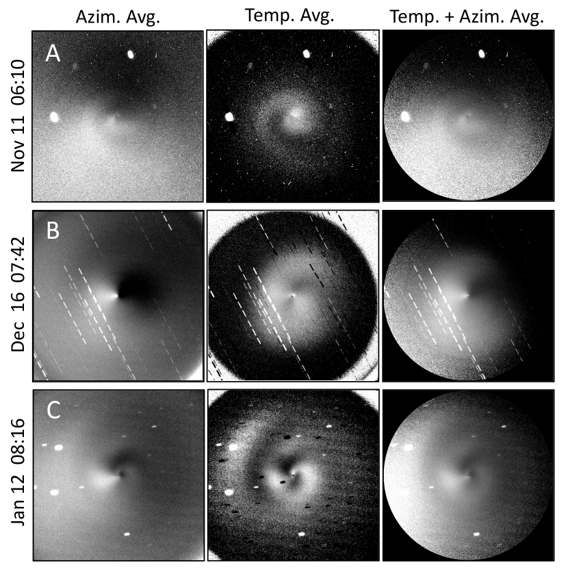
Figure 1: Examples of image enhancement techniques applied to sample images from three dates around perihelion. This figure also illustrates some of the basic morphology seen around perihelion, with two jets approximately 180° apart arising from the nucleus on each date. Images in rows A and C are 60,000 km across, while those in row B are 30,000 km across. North is up and East is to the left. The bright streaks are star trails, while the dark streaks in the rotational averaged column are the negative values produced by stars from the other temporally-combined images.

When comparing the coma morphology in the enhanced images, we find that the primary features remained consistent over multiple rotations (aside from changes in the viewing geometry). However, subtle, low-level features (e.g., faint arcs near the edge of the field) can sometimes exhibit notable differences, due to the effects of seeing and transparency variations, background sky removal, and even contrast display levels. Thus, caution should be taken in interpreting the differences in these low-level features.

3 Coma Morphology and Rotational Analysis

3.1 Feature Descriptions and Motions

We explored the dust morphology to determine how it might affect our CN analyses. On most observing runs, the typical underlying continuum is not significant (typically less than a few percent) when compared to the CN. Near close approach, the concentrations of dust near the optocenter can be detected in some of the enhanced CN images (see Knight et al. (2020) for more details). Fortunately, the dust morphology differs from the CN morphology (Figure 2) and essentially remains unchanging with rotation. Thus, when dust is detected, it should not affect our search for periodicity. An outburst detected on December 12, discussed further in Section 5, is one exception.

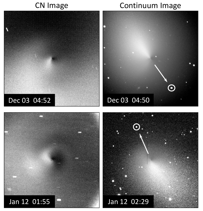
Figure 2: Comparison of sample CN and continuum images, showing that the dust features are usually not detected in the CN morphology. CN images are enhanced by division of an azimuthal averaged profile and the dust images are enhanced by division of a 1/$\rho$ profile. December images have a field of view of 30,000 km, January images of 60,000 km.

Sample CN images from each observing run are shown in Figure 3. Throughout our observations, the basic CN morphology is indicative of a nucleus with at least two isolated active areas. In general, one feature appears to have been active (at varying levels) throughout most of a rotation, while the second turned on and off with rotation. As viewed from Earth during the comet’s approach and recession, the jets produced spirals around the nucleus. The sense of rotation was clockwise pre-perihelion and counterclockwise post-perihelion, indicating that the Earth crossed the comet’s equator sometime around perihelion. In the weeks around perihelion, the structures from the two sources were broader (due to the small spatial scale caused by proximity to Earth) and often overlapped, confusing the interpretation of the morphology. At one point in the rotational phase, however, a corkscrew morphology is apparent, indicating that one of the jets was at a mid-level latitude, with the Earth outside the cone being swept out by that jet. At other phases, (e.g., the December 14 image in Figure 3) symmetric features are seen on opposite sides of the nucleus, suggesting that the other active region was near the equator, with its jet sweeping across the line of sight. The discontinuity introduced by the overlapping features around perihelion interferes with our ability to interpret the comet’s overall behavior. It is not clear from inspection of the data alone, whether the two jets seen pre-perihelion were the same as those seen post-perihelion, or if there were more than two active areas, with different sources turning off/on during the period of confused morphology. See Knight et al. (2020) for a more detailed depiction and analysis of the jet morphology.

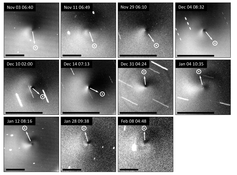
Figure 3: Sample image from each observing run, showing the typical progression of the morphology throughout the apparition (e.g., the spiral starts in the clockwise direction, exhibits a broad corkscrew at closest approach, and ends in the counterclockwise direction). Images are enhanced by dividing out an azimuthally averaged profile. North is up, East to the left, and the scale bar at the bottom is 20,000 km.

The radial distance of the arcs as a function of time/rotational phase reflects the projected velocity of the CN streaming outward from the active areas. In images from November 11-13 and January 12, we measured the radial distance of the arcs as a function of time at eight position angles (PAs) around the nucleus, and fit a linear function to each PA to estimate the gas velocities. In November, the highest velocity (presumably that with the smallest projection effect) was 0.62 km s^-1 at PA 180°, and in January, the highest velocity was 0.80 km s^-1 at a PA 90°. We also attempted these measurements with the mid-December runs, but our attempts to consistently define radially expanding features were difficult, due to the broad and overlapping morphology. In this case, we do not believe we obtained any measurements from which velocities can be reliably computed.

3.2 Rotational Phasing and Period Determination

We used the comet’s coma morphology as a tool for deriving the nucleus’ rotation period. This process assumes that the nucleus was in or near a state of simple rotation and that active areas producing the jets reacted to the solar irradiation in the same manner on every rotation. Thus, when a pair of images show the same morphology, it indicates that an integer number of rotations have passed between the two images. In practice, the morphology can be affected by changing illumination conditions, as the comet orbits the Sun, and changing viewing geometry, as the comet passes the Earth. Typically these changes are gradual and can be neglected for observations obtained over the course of a week or two, though during Wirtanen’s close approach to Earth, they become more pronounced. Because we have multiple observing runs between November 2018 and February 2019, we were able to derive independent rotation periods for different times throughout this window and use them to look for an evolution in the rotation state as the comet passed perihelion. For investigating the rotational phasing at different epochs, we combined our data into groups by individual observing runs (denoted by numbers in the Phase Group column in Table 1) and by neighboring inter-run groups, when the geometry does not change dramatically (denoted by letters).

We used two techniques to derive the period from the morphology, with two authors independently taking different approaches that resulted in consistent results. First, we know the rotation is always near 9 hr from previous work (e.g., Farnham et al., 2018; Jehin et al., 2018) and from numerous nights where we have $>$9 hr of coverage. With this constraint, one author searched by eye for one or more pairs of images from each group for which distinctive morphological features matched, and derived a period by assuming an integer number of rotations over the intervening time. Examples of these pairs are shown in Figure 4. This technique was used to provide initial working periods before results from the other, more rigorous technique was finalized. The accuracy from this pairwise fitting is dependent on how close in phase the image pairs end up, though the wealth of images allowed us to find matches close enough that the results agreed well with our other techniques.

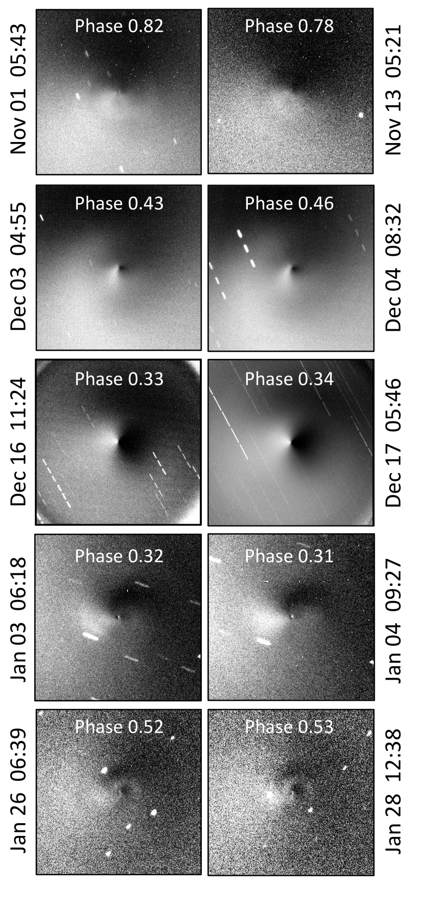
Figure 4: Representative pairs of CN images used to derive the rotation period. The close match between the features indicates an integer number of rotations in the interval. Images were enhanced by dividing out an azimuthally averaged profile. The phase designations are assigned, as discussed in the text, for reference.

In our second method, another author incorporated all of the data from a given run, assuming a period, computing the rotational phase for each image in that run, and then assembling an animated sequence with the images ordered by their respective phases. Zero phase is always defined at the comet’s perihelion date, 2018 December 12.931, so the phasing for a given run will change depending on the rotation period, and a particular phase for one run will not match that phase in runs with different periods. When the assumed period matches the actual period, a movie of this type should produce a smooth and continuous sequence of motion as the jet material flows outward from the nucleus. On the other hand, out-of-sequence frames (features jumping forward and back) indicate that the assumed period is not correct, and the number and size of these jumps grows as the difference between the assumed period and the actual period increases. We stepped through potential periods at intervals of 0.01 hr to look for acceptable sequences, which allowed us to define the range of valid periods for each run. Because the various enhancements reveal different aspects of the coma, we produced animations for all three of our techniques to confirm that they give a consistent result (these sequences can be found in animated GIF format at the University of Maryland (UMD) Digital Repository). Because this technique uses much more data than the pairwise matching, it provides a more precise result.

We recognize that there is an inherent subjectivity to defining an acceptable solution, especially in sequences where variable data quality, insufficient sampling rates, or changes in the viewing geometry can affect the apparent timing of a feature’s repetition. Thus, to avoid rejecting potentially valid periods, we used a conservative definition of “smooth” feature motions, pushing our solutions into the range where they may exhibit a few discontinuities to allow for these issues. These constraints are especially relaxed around the time of close approach, where the viewpoint was changing by as much as 4° per day. To minimize the effects of rapidly changing geometry for our December 13-17 observations, we separated the data into stepwise groups of 3 nights, deriving a separate period for each group. Although we obtained data on December 12 as well, these images were not included in this grouping due to the interference of an outburst. The division between acceptable and unacceptable values typically occurs when a period increment causes one or more pairs of key images to flip their sequence order, revealing an obvious discontinuity in the motion that cannot possibly be attributed to observing conditions or geometry changes. We define the measurement’s uncertainty as the point between the marginally acceptable value and the obviously unacceptable value (which effectively means our uncertainties are at the 3-$\sigma$ level). Thus, the center of our range of periods represents the smoothest sequence of images (our best estimate of the apparent period) while the uncertainties encompass any values that could be valid given the natural complexities of the data.

Finally, we combined data from the inter-run groups to refine the period even further. These groupings proved very powerful for several reasons. First, they increase the number of images used in each sequence, improving the phase coverage and overlap. Second, they extend the time baseline from a few days to a week or two, which, because small changes in period are amplified by the large number of intervening cycles, improves the precision. Finally, we have four observing runs in which we were unable to derive periods due to an insufficient number of images for reliable phasing, and combining each of these runs with a neighboring run allows us to incorporate these data. (Even a few images, when interleaved with a more complete sequence, can be very constraining.) For the early November and late January time frames, the geometry changes are minimal and thus these runs can be reliably combined. In early and late December, the changing geometry between runs, although not extreme, becomes noticeable, so we accepted a wider range of periods to account for these potential effects. Even so, the results from these inter-run combinations tend to be consistent with the individual runs from which they are comprised, but with smaller uncertainties.

The periods we derived are listed in Table 2 and plotted in Figure 5. These results suggest that the apparent period increased by $\sim$0.15 hr in the five weeks before perihelion, peaking at 9.14 hr before decreasing again by $\sim$0.2 hr in the eight weeks after perihelion. A 4th-order polynomial was fit to the measurements (coefficients: [9.138, -5.478$\times 10^{-5}$, -1.097$\times 10^{-4}$, 2.824$\times 10^{-7}$, 8.139$\times 10^{-9}$]) to provide a continuous representation of the period as a function of time, and we adopt the values from this curve to provide consistency in the different presentations of phased data throughout this paper. Figure Set 6 shows sequences of images from the individual observing runs, phased to the polynomial fit period for each run. Overall, the coma morphology repeats consistently over the course of single and multiple rotations (within the constraints introduced by the geometry changes) strongly suggesting that there are no noticeable effects produced by non-principal axis rotation. Thus, we conclude that the nucleus is in a state of simple rotation or nearly so.

Table 2: Rotation Periods Derived from Morphology

Phase	Date Range	$\Delta t_{\rm start}$	$\Delta t_{\rm end}$	Period (hr)			Poly.
Group		(day)	(day)	Min	Best	Max	(hr)
1	2018 Nov 01-04	–41.69	–38.60	8.92	8.98	9.05	8.97
A	2018 Nov 01-13	–41.69	–29.62	8.99	9.00	9.01	9.00
2	2018 Nov 09-13	–33.72	–29.62	8.98	9.03	9.07	9.03
—	2018 Nov 26-29	–16.73	–13.67	—	—	—	9.11
B	2018 Nov 26-Dec 06	–16.73	–6.65	9.09	9.13	9.17	9.12
3	2018 Dec 03-06	–9.82	–6.65	9.06	9.11	9.16	9.13
C	2018 Dec 03-10	–9.82	–2.52	9.12	9.14	9.16	9.13
—	2018 Dec 09-10	–3.85	–2.52	—	—	—	9.14
4	2018 Dec 13-15	0.13	2.46	9.07	9.12	9.17	9.14
5	2018 Dec 14-16	1.12	3.54	9.07	9.13	9.18	9.14
6	2018 Dec 15-17	2.15	4.54	9.06	9.12	9.17	9.14
—	2018 Dec 27-31	14.23	18.27	—	—	—	9.11
D	2018 Dec 27-2019 Jan 04	14.23	22.62	9.09	9.11	9.13	9.10
7	2019 Jan 03-04	21.15	22.62	9.06	9.09	9.13	9.09
E	2019 Jan 03-12	21.15	30.61	9.04	9.06	9.08	9.07
—	2019 Jan 12	30.15	30.61	—	—	—	9.05
F	2019 Jan 12-28	30.15	46.61	9.00	9.01	9.02	9.01
8	2019 Jan 26-28	44.16	46.61	8.94	8.98	9.02	8.97
G	2019 Jan 26-Feb 09	44.16	58.29	8.92	8.935	8.95	8.94
9	2019 Feb 08-09	57.25	58.29	8.88	8.94	8.99	8.91

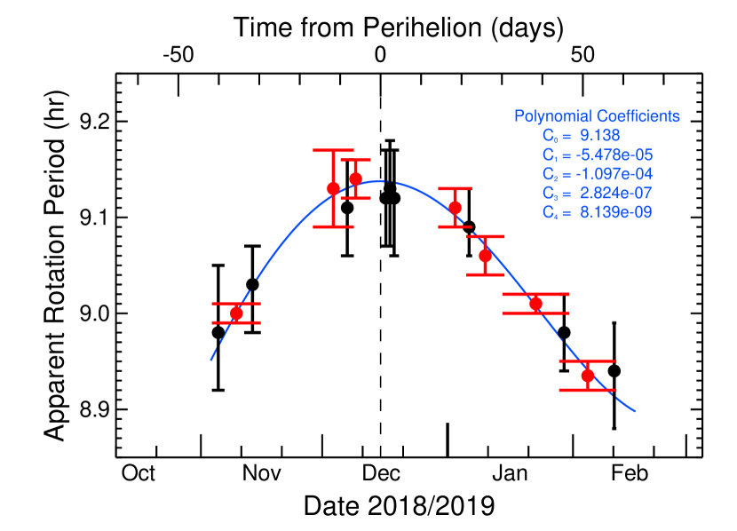
Figure 5: Rotation periods as a function of time derived from the image sequences. The vertical bar on each point indicates the range of acceptable solutions and the horizontal crossbars indicate the range of dates used for that sequence. Black symbols are solutions from individual runs, while the red symbols represent inter-run combination results. The blue curve shows a 4th order polynomial fit to the data.

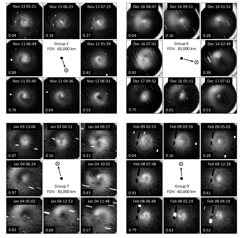
Figure 6: Representative looped image sequences showing the changing CN morphology as a function of rotational phase. Images were enhanced using the temporally averaged mask and phased to the polynomial fit values for each group (Table 2). North is up and East to the left. Full sequences for all groups of data can be found in animated GIF format at the UMD Digital repository https://drum.lib.umd.edu/handle/1903/26472.

3.3 Exploration of Synodic Effects

The fact that the changes in the apparent rotation periods are symmetric around the time of close approach raises the question of whether these changes are real or are they caused by synodic effects from the rapidly changing viewpoint? We explored this question both qualitatively and quantitatively. Some synodic effects arise when changes in the viewing geometry either shorten or lengthen the time for a reference longitude to return to the same spot relative to the observer. To evaluate the contributions from synodic effects, we look at the extremes where the geometry remained nearly constant or where it changed rapidly. In early November and late January/February, the comet’s motion was primarily toward/away from the Earth, with minimal change in viewpoint, so the apparent period from these times should be close to the sidereal period ($<$0.001 hr/rot). However, our measured periods are changing most rapidly during these epochs, suggesting that the sidereal period itself is evolving. In addition, our November measurement is different from that seen in February, which also argues that the sidereal period has changed through perihelion. At the other extreme, the biggest synodic effects should have occurred in the weeks surrounding closest approach when the viewing geometry changed most rapidly ($\sim$4°/day), yet our measurements show fairly constant values during this time frame. This contradicts the idea that the variations are produced by the viewing geometry.

We also performed more rigorous calculations to explore the viability of geometric effects producing our apparent measurements. The maximum possible synodic effects will occur if the fastest relative motion (e.g., at closest approach) corresponds to the time when the observer is at its highest latitude (where the cos(latitude) term magnifies the longitudinal motion). Because the sub-Earth latitude is determined by the spin axis orientation, we performed calculations for four different pole positions, one where the Earth skims along the comet’s equator, and three in which the sub-Earth point peaks at latitudes of 30°, 60°, and 90°. (Synodic effects for pole orientations in the opposite direction shorten the rotation period, which is the reverse of the trend we observed.) For each case, the synodic effects as a function of time are plotted in Figure 7 showing a trade-off between their magnitude and the duration that they act (i.e., as the peak increases, the curve gets narrower). Comparing these calculations to the results in Figure 5 shows that the changes seen in our measured periods cannot be due exclusively to the changing geometry. Not only are the magnitudes of the synodic effects too small (for all but the highest latitude cases) but their contributions are limited to a window around close approach that is too short to explain the trends that we see (confirming our qualitative analysis). We explored the synodic effects induced by the Sun for the same pole orientations, but these are substantially smaller than the Earth’s effects (peaking at $\sim$0.01 hr/rot), and so they too, are insufficient for explaining the observed period variations. Thus, we conclude that the changes seen in our measurements were actual changes in the nucleus’ rotation period.

Figure 7: Maximum possible shifts between Wirtanen’s apparent and sidereal periods due to the changing viewing geometry from the Earth. Synodic effects are plotted for four different pole orientations: one with the Earth at the equator (0°) and three that allow the Earth to reach 30°, 60°, and 90° latitude (see Section 3.3 for additional discussion). These results, when compared the results shown in Figure 5, show that the synodic effects are too small in magnitude and too narrow temporally to have produced the observed period changes.

4 CN Lightcurves and Rotational Analysis

Wirtanen’s lightcurves offered a second method for measuring the comet’s rotation period. Although somewhat hampered by calibration issues, as discussed below, this technique gives a separate measure of the spin period, providing a check on the morphology results. Furthermore, because the photometry is less dependent on the Earth’s motion, only the low-level solar synodic effects will apply, producing a result closer to the sidereal value at close approach.

Although we have good temporal coverage on many nights with both R (or r ^′) and CN filters, we chose to use the CN images because they consistently showed evidence of rotational variability (due to the higher gas velocities that allow the CN to leave the measuring aperture more rapidly, enhancing the amplitude of the variations). Because of weather and geometric circumstances, we had relatively few nights that could be fully calibrated (e.g., even on clear nights, the proximity to Earth means that, in much of our data, the coma fills the field of view, precluding an accurate measure of the sky background). Thus, for our period determinations, we decided to forego an absolute calibration and focus on the relative brightness changes and the timing of the peaks and troughs within a night. For this reason, we did not restrict our sample to photometric conditions but also accepted nights of fairly good quality that could be corrected, as discussed in section 4.1. The nights used in our lightcurve analyses are listed, with nightly conditions, in Table 3.

Table 3: Photometry Observing Conditions

Date	Avg. Bright.	$\Delta m$	$\sigma_{m}$	Seeing	Phase
	(mag)	(mag)	(mag)	(arcsec)	Groups
2018 Nov 11	12.506	—	0.002	3.0	2
2018 Nov 12	12.447	0.010	0.002	4.4	2
2018 Nov 13	12.373	—	0.002	4.1	2
2018 Dec 12	11.738	0.060	0.001	1.3	5
2018 Dec 13	11.762	0.025	0.001	2.7	5
2018 Dec 14	11.798	—	0.001	1.5	5
2018 Dec 16	11.760	0.035	0.001	1.2	5
2018 Dec 17	11.809	0.075	0.001	1.8	5
2019 Jan 03	11.866	—	0.002	4.4	7,E
2019 Jan 04	11.864	—	0.002	2.8	7,E
2019 Jan 12	12.440	0.040	0.001	2.2	E,F
2019 Jan 26	12.982	0.015	0.003	3.3	8,F,G
2019 Jan 28	12.997	-0.005	0.003	2.2	8,F,G
2019 Feb 08	13.630	—	0.003	4.4	9,G
2019 Feb 09	13.708	0.030	0.003	3.3	9,G

4.1 Photometric Calibrations

To assemble our lightcurves, we started with the bias-removed and flat-fielded images, centroided on the optocenter of each image and performed photometry using a 10-arcsec radius aperture. This aperture size was used throughout the apparition as a compromise between the need for an aperture large enough to minimize the effects of seeing variations, but small enough to enhance the rotational variability. (Because of the large range in $\Delta$, an aperture of fixed physical size at the comet was impractical.) This results in a different fraction of the coma being measured on each night, but as our objective is the variability within the night, this is a minor concern.

The sky background level was estimated using an annulus centered on the optocenter. The outer radius is set independently on each night, using the maximum dimension that can be used throughout that night (avoiding chip edges, vignetting, etc.), while the width of the annulus was $\sim$100 pixels. Coma fills the field in December (and into November and January), so the sky level is usually over-estimated in our measurements, but because it tends to be stable during each night, it should have a minimal effect on the rotational variability analyses.

On photometric nights, we used measured coefficients to correct for extinction. The remaining nights used coefficients from the same run, if available, or typical coefficients for the telescope as a last resort. On runs where the sky contamination was minimal, we could also use field stars to correct for the relative extinction due to airmass and thin cirrus throughout a night (e.g., Knight et al., 2011, 2012; Schleicher et al., 2013; Eisner et al., 2017). Such tweaks were not possible during December and early January, due to rapid proper motions and extreme coma contamination, so there may be residual extinction trends on those nights. Fortunately, the majority of those data were acquired at airmass $<$1.5, so the trends are unlikely to affect our interpretations.

Typically, our final task was the removal of underlying continuum from the calibrated CN images Farnham et al. (2000). However, as noted earlier, the continuum signal in most of our observations was minimal, and because we were unable to remove the continuum from all of our data, we decided to stay consistent and not remove it from any of our data. If any signal from the dust is detected, it would slightly dampen the amplitude of the lightcurve variations, but should have minimal effect on the timing of the peaks and troughs, and thus the period determinations.

4.2 Photometry Results

Our nightly CN lightcurves are plotted in Figure 8 (the photometry measurements are available as Data Behind the Figure). Data points that are filled in gray denote that an extinction correction derived from field star extinction was applied during the calibration process. A number of nights (December 16, January 3 & 4, February 8, etc.) had regular, high quality data spanning $\gtrsim$9 hr. Although these nights are valuable for confirming the $\sim$9 hr period and for permitting assessment of the full lightcurve shape in one night’s observations, they are of limited value in deriving precise rotation periods. For period determination, we phased multiple nights’ data (combined as noted in the Phase Groups column of Table 3) to construct more extensive lightcurves.

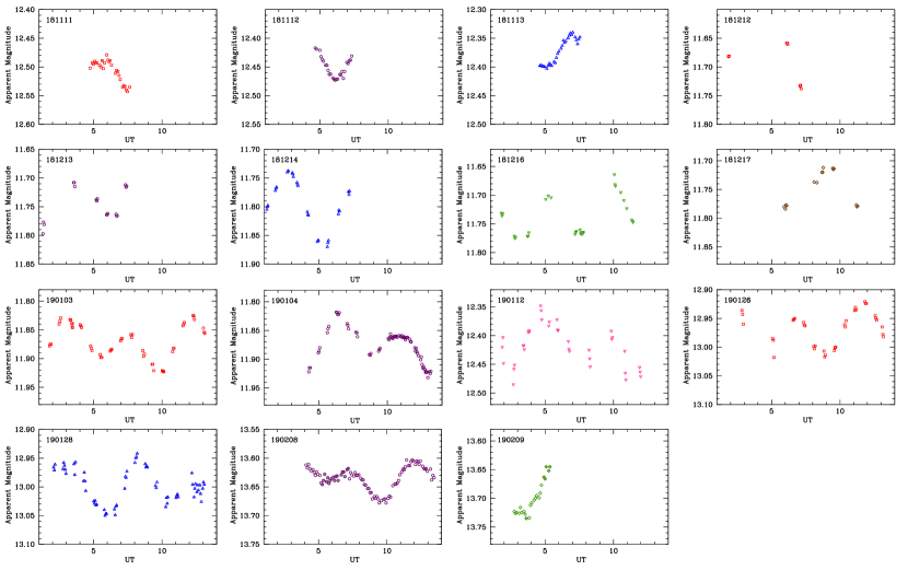
Figure 8: Lightcurves segments from our nightly observations (dates listed in YYMMDD format). Points filled in grey have been corrected for extinction using field star comparisons. Observation times have been corrected for light travel time. The CN magnitude data used to produce these plots is included as Data Behind the Figure.

We determined rotation periods by eye as discussed in Schleicher & Knight (2016), phasing the lightcurves to different periods and looking for the best alignment of the overlapping segments. While evaluating the best fits, we allowed arbitrary vertical offsets of nightly segments (listed in Table 3) to account for any brightness differences arising from our lack of absolute calibration. After the best period was found, we estimated its uncertainties by exploring how much the period could be changed before the lightcurves showed an obvious misalignment (roughly a 3-$\sigma$ uncertainty). Uncertainties are dependent on the baseline of the observations, with a longer span of observations producing better precision, but the shape of the lightcurve changes over time, so we limited our measurements to groups of data spanning less than two weeks. The periods derived from our lightcurve analyses are listed in Table 4 and plotted in Figure 9. These results are in excellent agreement with those derived from our morphology analysis, but with larger uncertainties due to the calibration issues. This confirms that the comet’s rotation rate was changing, and also indicates that the synodic effects introduced by the Earth’s motion were minimal.

Table 4: CN Lightcurve Properties

Phase	Nights Used	Mid-Date	Period	P. Range	Poly. Fit	L. Range	Phase
Group			(hr)	(hr)	(hr)	(mag)	Sep.
2	Nov 11, 12, 13	Nov 12.256	9.00	8.75–9.15	9.03	0.065	0.50
5	Dec 12, 13, 14, 16, 17	Dec 14.774	9.15	9.06–9.33	9.14	0.125	0.54
7	Jan 3, 4	Jan  3.812	9.11	8.98–9.19	9.09	0.105	0.54
E	Jan 3, 4, 12	Jan  7.787	9.07	9.04–9.12	9.07	0.105	0.54
F	Jan 12, 26, 28	Jan 20.312	9.02	8.99–9.05	9.01	0.095	0.52
8	Jan 26, 28	Jan 27.332	9.04	8.86–9.20	8.97	0.095	0.52
G	Jan 26, 28, Feb 8, 9	Feb  2.171	8.93	8.91–8.95	8.94	0.090	0.50
9	Feb 8, 9	Feb  8.697	8.85	8.75–9.05	8.91	0.075	0.50

Our multi-night phased lightcurves are shown in Figure 10. Because the derived periods are consistent between our techniques, we have adopted the values from our 4th order polynomial for displaying our photometry plots as well, which allows us to compare the relative phases in the lightcurves to the morphology from the same time. (The results show little difference from those using the periods derived from the lightcurve analysis.) These plots reveal a double-peaked lightcurve, with the variations produced by cometary activity. Although the shape and the peak-to-peak range vary throughout the apparition, one peak is consistently shallower than the other. Table 4 lists the lightcurve ranges, which vary from $\sim$0.065–0.125 mag and the phase separation from the higher to the lower peak. These separations are not equidistant, but vary between 0.50 and 0.54, with the biggest separations correlated with close approach.

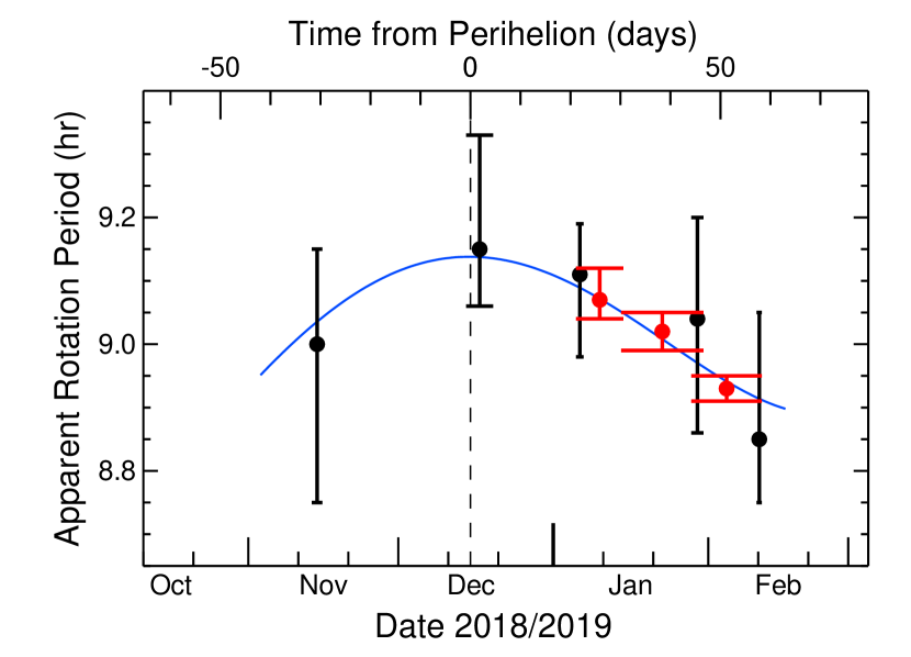
Figure 9: Rotation periods as a function of time derived from the photometric lightcurves, showing the same trends as in the morphology-derived periods, but with larger uncertainties. The error bars and colors represent the same information stated in Figure 5. The blue curve reproduces the 4th order polynomial derived from the morphology sequences.

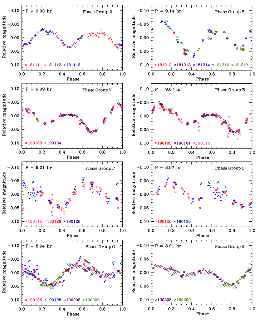
Figure 10: Multi-night phased lightcurves showing the comet’s variability. Symbols match those used in Figure 8, though in this plot, filled points indicate data that were obtained during outbursts. For January 28, triangles pointing upward denote measurements from the first four hours of the night, while those pointing downward designate the rest of the night. Periods from the 4th order polynomial fit (listed in each panel) were used for the phasing. Because the different periods are all referenced to our fiducial point at perihelion, a given phase in one panel does not match that in other panels.

5 Outburst Events

Our observations include two significant outbursts, one on December 12 and a second on January 28. The changing dust morphologies, seen in broadband R filter sequences, are shown in Figure 11.

The first outburst was dominated by a bright, “V”-shaped extension to the Northeast. There is also material enveloping the Northwest and South, though it is fainter and fades more rapidly. Although one arm of the “V” was in the anti-sunward direction, the other was not, and as there is no curvature toward the tail, we conclude that radiation pressure was not a significant issue at the observed distances. Furthermore, if we assume the outburst was in sunlight at the time, then the small solar phase angle suggests that there are likely to be notable projection effects toward the Earth. This is supported by the fact that ejecta were detected at azimuths almost entirely around the nucleus. The linear nature of the arms of the “V” also suggests that there was little effect from rotation and thus the event was of short-duration.

We measured the motion of the outer apex of the “V” and derived a projected expansion velocity 68$\pm$5 m s^-1. Extrapolating this measurement back to the nucleus indicates the outburst began December 12 at 00:13 UT $\pm$7 min. Because we see outburst material extending into the optocenter throughout our December 12 observations, we can constrain the slowest moving material to speeds $<$20 m s^-1 (projected, and assuming an impulsive outburst). The dust ejected in the “V” feature was bright enough to dominate the signal, even in the CN filter, throughout the rest of the night. There is no obvious sign of the outburst in the morphology on December 13, though given the derived speeds, diffuse residual material is likely to be present.

The second outburst, on January 28, exhibited a narrow stream of material flowing to the South with a slight curvature toward the anti-solar direction. The curvature cannot be the result of rotation (which would imply an extended period of emission), because it is opposite the direction of the spirals seen in the CN features. This suggests that the ejecta is composed of small dust grains that are rapidly being pushed tailward by solar radiation pressure. The leading edge of the material has a projected velocity of 162$\pm$15 m s^-1, which indicates the event began January 27 at 20:01 UT $\pm$30 min. This outburst is notably fainter than the December event, and is seen in our R filter images. Although there is no indication of the dust stream in our enhanced CN images, the first few hours of photometry are $\sim$0.03 mag brighter than the measurements 9 hr (one rotation) later (cf. phase 0.5 in the January 26 & 28 plot of Figure 10). This suggests that the photometry is sensitive to a secondary contribution from the outburst, possibly as diffuse, axially symmetric material, similar to the phenomena seen during an outburst in Wirtanen on 2018 September 26 (Farnham et al., 2019), that is removed in our enhancements.

We explored additional aspects of these outbursts using our Monte-Carlo model, with results presented by Knight et al. (2020). Kelley et al. (2020) also provide additional analyses.

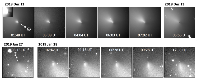
Figure 11: R-band images showing the dust morphology in the December 12 and January 28 outbursts. Images are enhanced by dividing out a 1/$\rho$ profile. The December frames are 10,000 km across and the January frames are 30,000 km across. The inset in the first panel shows the inner 3,000 km of coma with a harsher stretch to reveal the faint ejecta to the Northwest and South. The December 13 and January 27 images show the closest outburst-free coma for comparison.

6 Discussion and Summary

6.1 CN Coma Morphology

The basic morphology revealed in our enhanced CN observations consistently shows two jets that were tracked throughout the apparition. One of the jets remained active over most of a rotation, while the other appeared to turn on and off with rotation. Although we can’t conclude that the two jets arose from the same active areas throughout the apparition, the sources always appeared roughly half a rotation apart suggesting that they could be the same. Early and late in our observations, the jets produced spirals around the nucleus, but they rotated clockwise pre-perihelion and counterclockwise post-perihelion, suggesting that the Earth crossed the comet’s equator around perihelion. Samarasinha et al. (1996) originally argued that the nucleus of comet Wirtanen was likely in a non-principal axis (NPA) rotation state, but later work (e.g., Gutiérrez et al., 2005) suggested that the angular momentum might change, without resulting in an excited rotation state. Indeed, we see no evidence for NPA rotation in our data. Previous morphology analyses (e.g., Knight & Schleicher, 2011; Samarasinha et al., 2011) have shown that coma morphology can be a powerful tool for revealing evidence of NPA states, but the features in our image sequences, when phased to the relevant period, remain consistent from one rotation to the next and from one night to the next. Thus, we conclude that Wirtanen’s nucleus is in a near-simple rotation state. Our measured CN velocities, 0.62 km s^-1 in mid-November ($r_{H}$=1.14 au) and 0.80 km s^-1 in mid-January (1.13 au) are consistent with other measurements of gas outflow for comets with similar gas production and heliocentric distance (e.g., Tseng et al., 2007; Lee et al., 2015).

We used our CN morphology to constrain Monte-Carlo models of the coma, to derive additional characteristics of the comet. This work is presented by Knight et al. (2020), and the results that the two studies have in common are in general agreement.

6.2 CN Lightcurves

Our lightcurves are all double peaked, suggesting that there are two primary active areas on the nucleus. (Unlike in asteroid lightcurves, where a double peaked lightcurve represents the changing cross-sectional surface area of a spinning body, the variations in our coma lightcurves are produced by the changing production rates of active areas as they rotate into and out of sunlight.) The phase separation ($\sim$0.52 from the primary to the secondary peak) suggests the two active areas are separated by an effective longitude $\sim$190° (or $\sim$170° in the other direction). This two-source configuration is consistent with the structures we see in the morphology.

Comparing our phased lightcurves to the enhanced morphology images helps in the interpretation of the lightcurve details. The timing of a peak typically occurs $\sim$0.1 phase after the initial appearance of a jet in the morphology, with the brighter peak matching the jet that remains active throughout the full rotation. The phase offsets are the result of the delay between the start of emission and the point at which material exits the aperture. This timing changes somewhat over the course of the apparition, because of the changing dimensions of the 10-arcsec aperture at the comet. The changing shape of the lightcurve and relative brightnesses of the peaks is caused by the viewpoint evolution (where the spirals early and late exit the aperture more rapidly than the face-on material around close approach) combined with changes in the relative production rates of the two sources. These same effects are likely the cause of the variations in the phase separation between the high and low peak (0.50 to 0.54).

Although the relevant dates are not absolutely calibrated, we do detect evidence of the two outbursts in our lightcurve measurements. There are only three sets of measurements, spanning half a rotation, from December 12. They seem to match well with the phased lightcurve, but the entire night requires an offset of $\sim$0.1 mag — significantly higher than any other night of comparable quality — to bring the data into line with the following nights. This shows that the CN dominates the variability of the lightcurve, but has underlying continuum from the outburst that systematically increases the brightness. The data quality on January 28 is lower, with more scatter at various times during the night, but the outburst still affects the lightcurve. As noted in Section 5, the first few hours of photometry are $\sim$0.03 mag brighter than the same phase captured later in the night, suggesting that we see some contribution from the outburst.

6.3 Rotation Period

We used three different techniques to measure Wirtanen’s apparent rotation period at different epochs. All of these techniques are in excellent agreement and show that the period increased from our initial measurement of 8.98 hr in November to 9.14 hr at perihelion. After perihelion, it decreased again, reaching our final measurement of 8.94 hr in February. Measurements from TRAPPIST telescopes spanning 12.5 hr on 2018 December 9-10 showed a period 9.19$\pm$0.05 hr (Jehin et al., 2018; Moulane et al., 2019), which agrees with our results to within the errorbars. Two other measurements of Wirtanen’s rotation period exist, both measured from sparse data sets obtained in 1996. Meech et al. (1997) report a 7.6 hr period from 1996 August 17/18 (-209 day from perihelion), and Lamy et al. (1998) report a period of 6.0$\pm$0.3 hr from 1996 August 28 (-198 day). These results are discussed further below.

Our measurements represent apparent periods, but we showed that synodic effects are too small to produce the observed changes, and thus conclude that the nucleus is indeed changing its rotation rate with time. This indicates that the comet’s activity is producing significant torques, with the net direction of those torques changing direction around the time of perihelion. Our observations suggest there are two primary active areas, separated by $\sim$170°. It is not difficult to conceive of scenarios, given a non-spherical nucleus, where seasonal effects change the relative levels of activity of the sources, reversing the direction of the torque. See our companion paper (Knight et al., 2020) for additional exploration of this issue. Similar behavior was seen in Rosetta measurements, where comet 67P/Churyumov-Gerasimenko (C-G) was observed to initially increase its rotation period by $\sim$0.03 hr before the net torques reversed direction and decreased the period by $\sim$0.37 hr (Keller et al., 2015; Kramer et al., 2019).

The trends in our measurements suggest that the period is already increasing in November, and continues to decrease in February, thus neither of these measurements represents an end state to the period changes, though the February measurement, at +57 day, already hints that the rate of change is slowing. If we assume that the torques act in proportion to water production, then by the end of March ($\sim$+100 day), where production rates are $<$10% of their peak value (Knight et al., 2020), the torques should largely be gone. As both the production rates and the period changes in Wirtanen appear to be symmetric around perihelion (ignoring synodic effects), we can further assume that the period began increasing at -100 day (early September). It is notable that the window within 100 day of perihelion is also where C-G exhibited the bulk of its changes (Kramer et al., 2019). If we extrapolate the ends of the curve in Figure 5 so they flatten out at $\pm$100 days, then the period at these extremes is likely to be around 8.8 hr. Thus, the period exhibits a maximum excursion of $\sim$4% around perihelion, but it has nearly the same value at both the start and end of the apparition.

With this in mind, we can evaluate the periods measured in 1996. The 7.6 and 6.0 hr periods (Meech et al., 1997; Lamy et al., 1998) represent changes of 16% and 45%, respectively, from our starting period, over four apparitions. Barring any major alterations in the comet’s torques due to activity or pole orientation, neither of these measurements is consistent with our result. Given that they also disagree with each other, though they were obtained only 11 days apart, we suggest that at least one of the results (most likely the 7.6-hr ground-based measurement) may have contained more coma contamination than assumed, and thus produced faulty results. As noted, the general trends that we see in 2018 are insufficient to alter the period from 6 hr to 9 hr in four apparitions, but we cannot preclude unusual activity in the intervening years that could have produced these changes, and there is evidence for potentially significant outburst activity during the 2002 apparition (Combi et al., 2020) that perhaps could account for changes on this scale.

The 2018/2019 apparition of comet Wirtanen, with an historically close approach to the Earth, provided an excellent opportunity for studying this important comet in detail. We used this opportunity to acquire a wealth of observations using both broadband and narrowband data, from which we derived a number of important characteristics of the comet. Our first results are presented in this document and in our companion paper by Knight et al. (2020) and we expect to continue our analyses in the future.

References

- A’Hearn et al. (2011) A’Hearn, M. F., Belton, M. J. S., Delamere, W. A., et al. 2011, Science, 332, 1396
- Boehnhardt et al. (2002) Boehnhardt, H., Delahodde, C., Sekiguchi, T., et al. 2002, A&A, 387, 1107
- Combi et al. (2020) Combi, M. R., Mäkinen, T., Bertaux, J. L., et al. 2020, Planetary Science Journal, Accepted for publication
- Combi et al. (2019) Combi, M. R., Mäkinen, T. T., Bertaux, J. L., Quémerais, E., & Ferron, S. 2019, Icarus, 317, 610
- Cowan & A’Hearn (1979) Cowan, J. J., & A’Hearn, M. F. 1979, Moon and Planets, 21, 155
- Eisner et al. (2017) Eisner, N., Knight, M. M., & Schleicher, D. G. 2017, AJ, 154, 196
- ESA (1994) ESA. 1994, Rosetta Science Management Plan, ESA/SPC(94)37
- Farnham et al. (2019) Farnham, T. L., Kelley, M. S. P., Knight, M. M., & Feaga, L. M. 2019, ApJ, 886, L24
- Farnham et al. (2018) Farnham, T. L., Knight, M. M., & Schleicher, D. G. 2018, Central Bureau Electronic Telegrams, 4571, 1
- Farnham & Schleicher (1998) Farnham, T. L., & Schleicher, D. G. 1998, A&A, 335, L50
- Farnham et al. (2000) Farnham, T. L., Schleicher, D. G., & A’Hearn, M. F. 2000, Icarus, 147, 180
- Groussin & Lamy (2003) Groussin, O., & Lamy, P. 2003, A&A, 412, 879
- Gutiérrez et al. (2005) Gutiérrez, P. J., Jorda, L., Samarasinha, N. H., & Lamy, P. 2005, Planet. Space Sci., 53, 1135
- Jehin et al. (2018) Jehin, E., Moulane, Y., Manfroid, J., & Pozuelos, F. 2018, Central Bureau Electronic Telegrams, 4585, 1
- Keller et al. (2015) Keller, H. U., Mottola, S., Skorov, Y., & Jorda, L. 2015, A&A, 579, L5
- Kelley et al. (2020) Kelley, M. S. P., Farnham, T. L., Li, J.-Y., et al. 2020, Planetary Science Journal, This volume, Submitted
- Knight et al. (2011) Knight, M. M., Farnham, T. L., Schleicher, D. G., & Schwieterman, E. W. 2011, AJ, 141, 2
- Knight & Schleicher (2011) Knight, M. M., & Schleicher, D. G. 2011, AJ, 141, 183
- Knight et al. (2020) Knight, M. M., Schleicher, D. G., & Farnham, T. L. 2020, Planetary Science Journal, submitted
- Knight et al. (2012) Knight, M. M., Schleicher, D. G., Farnham, T. L., Schwieterman, E. W., & Christensen, S. R. 2012, AJ, 144, 153
- Kobayashi & Kawakita (2010) Kobayashi, H., & Kawakita, H. 2010, PASJ, 62, 1025
- Kramer et al. (2019) Kramer, T., Läuter, M., Hviid, S., et al. 2019, A&A, 630, A3
- Lamy et al. (1998) Lamy, P. L., Toth, I., Jorda, L., Weaver, H. A., & A’Hearn, M. 1998, A&A, 335, L25
- Lee et al. (2015) Lee, S., von Allmen, P., Allen, M., et al. 2015, A&A, 583, A5
- Meech et al. (1997) Meech, K. J., Bauer, J. M., & Hainaut, O. R. 1997, A&A, 326, 1268
- Moulane et al. (2019) Moulane, Y., Jehin, E., José Pozuelos, F., et al. 2019, in EPSC-DPS Joint Meeting 2019, Vol. 2019, EPSC–DPS2019–1036
- Protopapa et al. (2014) Protopapa, S., Sunshine, J. M., Feaga, L. M., et al. 2014, Icarus, 238, 191
- Samarasinha & Larson (2014) Samarasinha, N. H., & Larson, S. M. 2014, Icarus, 239, 168
- Samarasinha et al. (2011) Samarasinha, N. H., Mueller, B. E. A., A’Hearn, M. F., Farnham, T. L., & Gersch, A. 2011, ApJ, 734, L3
- Samarasinha et al. (1996) Samarasinha, N. H., Mueller, B. E. A., & Belton, M. J. S. 1996, Planet. Space Sci., 44, 275
- Schleicher & Farnham (2004) Schleicher, D. G., & Farnham, T. L. 2004, in Comets II, ed. M. H. Festou, U. Keller, & H. Weaver (Tucson: University of Arizona Press), 449–469
- Schleicher & Knight (2016) Schleicher, D. G., & Knight, M. m. 2016, AJ, 152, 89
- Schleicher et al. (2013) Schleicher, D. G., Knight, M. M., & Levine, S. E. 2013, AJ, 146, 137 (8pp)
- Tseng et al. (2007) Tseng, W. L., Bockelée-Morvan, D., Crovisier, J., Colom, P., & Ip, W. H. 2007, A&A, 467, 729