Exploring and comparing temporal clustering methods

Abstract

Description of temporal networks and detection of dynamic communities have been hot topics of research for the last decade. However, no consensual answers to these challenges have been found due to the complexity of the task. Static communities are not well defined objects, and adding a temporal dimension renders the description even more difficult. In this article, we propose a coherent temporal clustering method: the Best Combination of Local Communities (BCLC). Our method aims at finding a good balance between two conflicting objectives : closely following the short time evolution by finding optimal partitions at each time step and temporal smoothness, which privileges historical continuity. We test our algorithm on two bibliographic data sets by comparing their mesoscale dynamic description to those derived from a (static) simple clustering algorithm applied over the whole data set. We show that our clustering algorithm can reveal more complex dynamics than the simple approach and reach a good agreement with expert’s knowledge.

Keywords: dynamic community detection, dynamic systems visualization, dynamic community assessment, temporal networks, bibliographic networks

1 Introduction

Networks are a convenient way to represent real-world complex systems, such as social interactions Newman (2003),Onnela et al. (2007), metabolic interactions Boccaletti et al. (2006), the Internet/world wide web Pastor-Satorras & Vespignani (2001), transportation systems Dall’Asta et al. (2006); Barthélemy (2011), etc. For several systems it is interesting to find and describe areas of the network which are more densely connected, i.e. the communities of the network. In 20 years of complex networks history extensive work was conducted on community detection in static - non evolving - networks, see Newman (2006); Blondel et al. (2008); Fortunato & Barthélemy (2007) and the review Fortunato & Hric (2016) for an overview on community detection in static graphs.

However, many networks have a temporal dimension and need a dynamic mesoscopic description at risk of non-negligible information losses if studied as static networks. Therefore the description of large temporal graphs has been a hot topic of research for the last decade, see the excellent reviews Holme & Saramäki (2012) and Holme (2015) for a complete description of temporal networks. Most recently the detection of dynamic communities, that is communities on temporal networks, has become one of the main interests in network science, as temporal networks require to adapt the methods of static community detection. So far no consensual method was found and around 60 methods have been proposed to try to detect dynamic communities evolving with temporal networks. A total of four published reviews try to classify and summarize them Aynaud et al. (2013), Hartmann et al. (2016), Masuda & Lambiotte (2016) and Rossetti & Cazabet (2018).

In Rossetti & Cazabet (2018), these methods are classified into 3 main categories: (a) instant optimal, (b) temporal trade-off and (c) cross-time. These methods aim to detect clusters at different times t, i.e. for many snapshots of the temporal network. As these clusters are only dependent on the state of the network at time t, it is then necessary to match the communities at different t with some similarity measures, e.g. Jaccard based Morini et al. (2017); Lorenz et al. (2018); Greene et al. (2010), core-node Wang et al. (2008). Methods in category (b) define clusters at t depending on current and past states of the network. Clusters are incrementally temporally smooth. However such methods are subject to drift as clusters are added up to each other locally. There is no compromise between temporal smoothness and ’optimal’ partition at time $t$, see for example Rossetti et al. (2017); Guo et al. (2014); Görke et al. (2010, 2013). Finally, in category (c) clusters at $t$ depend on both past and future states of the network, see Duan et al. (2009); Mucha et al. (2010); Matias & Miele (2016); Ghasemian et al. (2016). Clusters are completely temporally smooth and not subject to drift, but they do not respect causality as communities at $t$ are determined using network’s information at $t+n$, i.e. communities at time $t$ can change depending on what comes next, which makes these methods inappropriate for use on-the-fly.

In this article, we present a new tool to achieve a mesoscopic description of dynamic networks, which tries to find a good compromise between ’global’ and ’local’ methods. We apply our method on two data sets of scientific articles, to show how it can describe the emergence and evolution of scientific disciplines. The main difficulties for meta-community detection methods are twofold: Finding the right temporal smoothing and quantifying the ‘stability’ of communities. It is difficult to distinguish if changes between snapshots are due to structural evolution of the community or algorithm instability, as static community detection methods used at each time $t$ can find different communities for a same topology (see Rossetti & Cazabet (2018) for a complete description of pros and cons of each clustering category). Here, we propose an algorithm which aims to find a good balance between temporal inertia (smoothness) and ‘optimal’ partition at any given time $t$. We compare this method to the most basic approach, which optimizes the modularity of the aggregated network using the Louvain algorithm Blondel et al. (2008). The latter can be assimilated to a category (c) method in Rossetti & Cazabet (2018). We then describe the methods to analyze differences between partitions: mutual information (MI) measures and bipartite network (BN) representations. We show that MI based measures are interesting but give a limited amount of information on how different two partitions are, whereas bipartite network representation allows to see how streams split between partitions. We used the methods on two bibliographic data sets: (1) the scientific publications of a scientific institution, ENS Lyon and (2) publications related to the emergence of a new mathematical tool, the ’wavelets’. We show that the global approach represents a good approximation when the dynamics is simple, i.e. when there are mainly parallel streams without much interaction, as in the ENS Lyon case. However, when the dynamics is more complex (and interesting), when many communities are born, die, split or merge, one needs a more sophisticated approach, and we show that our algorithm performs well compared to an expert-based dynamics.

2 Methods

We start by presenting the two building blocks used in the algorithms we want to compare: how we define and partition a Bibliographic Coupling (BC) network and how we match clusters from successive time periods to create ‘streams’ (temporal meta-clusters). We then introduce the BiblioMaps platform used for visualizing dynamic communities and finally we present two standard methods to compare partitions derived from the different methods : Normalized Mutual Information and Bipartite Networks.

2.1 Bibliographic Coupling partitioning

Given a set of publications on a given period, a Bibliographic Coupling (BC) network can be defined based on the relative overlap between the references of each pair of publications. More specifically, we compute Kessler’s similarities $\omega_{ij}=R_{ij}/\sqrt{R_{i}R_{j}}$, where $R_{ij}$ is the number of shared references between publications $i$ and $j$ and $R_{i}$ is the number of references of publication $i$. In the BC network, each publication corresponds to a node and two publications $i$ and $j$ share a link of weight $\omega_{ij}$. If they don’t share any reference, they are not linked ($\omega_{ij}=0$); if they have an identical set of references, their connexion has a maximal weight ($\omega_{ij}=1$). Here, we consider that the link between two publications is only meaningful if they share at least two references and we impose $\omega_{ij}=0$ if they share only one reference.

We use weighted links to reinforce the dense (in terms of links per publication) regions of the BC networks. This reinforcement facilitates the partition of the network into meaningful groups of cohesive publications, or communities. We measure the quality of the partition with the modularity Q (eq. 1), a quantity that roughly compares the weight of the edges inside the communities to the expected weight of these edges if the network were randomly produced:

$$Q=\frac{1}{2\Omega}\sum_{i,j}\left[\omega_{i,j}-\frac{\omega_{i}\omega_{j}}{2\Omega}\right]\delta\left(c_{i},c_{j}\right),$$ (1)

where $\omega_{i}=\sum_{j}\omega_{ij}$ is the sum of the weights of the edges linked to node i, $c_{i}$ and $c_{j}$ are the communities containing respectively nodes $i$ and $j$, $\delta$ is the Kronecker function ($\delta(u,v)$ is 1 if $u=v$ and 0 otherwise) and $\Omega=\frac{1}{2}\sum_{ij}\omega_{ij}$ is the total weight of edges. We compute the graph partition using the efficient heuristic algorithm presented in Blondel et al. (2008).

2.2 Matching communities from successive time periods

Given the sets of communities $\{C_{1}^{t},...C_{k_{t}}^{t}\}$ in each time window $t$, the problem at hand is to identify a set of relevant historical communities, or streams, that correspond to a chain of communities from successive time periods (at most one per period). In order to decide which community of a given period should be added to a chain of communities from previous periods, we need to use some measure of the similarity between communities from different time periods. A standard measure is the Jaccard index, which computes the proportion of shared nodes between clusters of successive and overlapping periods (see e.g. Claveau & Gingras (2016); Morini et al. (2017)). One drawback of this measure is the need to use overlapping periods which implies that there is no bijection between the publications and the streams (a given publication can belong to several streams).

Here, we take advantage of the fact that links can be computed between nodes from different time periods (publications from different periods can have common references). We could for example define a similarity measure between two clusters $C_{a}$ and $C_{b}$ from different periods either by the total sum of the links between pairs of publications from these clusters $\Omega_{a,b}=\sum_{i\in C_{a},j\in C_{b}}\omega_{i,j}$ or by a normalized version of this sum $\omega_{a,b}=\Omega_{a,b}/|C_{a}||C_{b}|$, which is comprised between 0 and 1. While these two measures may appear quite intuitive, each of them has some drawbacks as well: using $\Omega_{a,b}$ may bias the construction of the streams by linking two ‘large’ (in terms of publications) but rather dissimilar (in terms of shared references) clusters. On the opposite, using $\omega_{a,b}$ may create some biases by linking two very similar clusters of very different sizes rather than the two clusters that have the second-best similarity and have similar sizes. To be coherent with our construction of clusters (maximizing the modularities within each time period), we propose here to use a modularity-based concept to match clusters from successive time periods. The similarity measure we use is thus $\delta Q=\Omega_{a,b}-\Omega_{a}\Omega_{b}/2\Omega_{A,B}$ which corresponds to an increase in the modularity of the BC network built from the two periods $A$ and $B$ when, starting from partitions defined on each period, clusters $a$ and $b$ are merged.

Matching Algorithm

Only compare pairs of communities $(a,b)$ with a minimum similarity $\omega_{a,b}>\Theta=10^{-6}$.

Define the best match of each cluster by the one maximizing $\delta Q$.

for each temporal window do

       Define the predecessor of each cluster as its best match from the previous time period.

       Define the successor of each cluster as its best match from the next time period.

end for

Two clusters are said to be paired if they are predecessors / successors of each other.

If a cluster is not the successor of its predecessor, we have a split.

If a cluster is not the predecessor of its successor, we have a merge.

Streams are defined as chains of paired clusters.

An illustration of this algorithm is given in Figure 1.

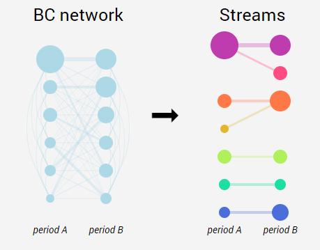
Figure 1: Matching clusters from successive time periods. We start with the BC network built from clusters of publications detected independently in periods A and B. For each cluster $a$ of period A and cluster $b$ of period B, we compute the modularity change $\delta Q_{ab}$ obtained by grouping these two clusters in the 2-periods BC network. The ‘successor’ of cluster $a$ is defined as the cluster $b$ from period B maximizing this quantity and the ‘predecessor’ of cluster $b$ is defined as the cluster $a$ from period B maximizing this quantity. In the stream visualisation, ‘paired’ clusters (successor / predecessor of each other) are represented on the same y-position, and we only show the BC links between successors or predecessors, which highlight dynamical events such as merge and splits. In these figures, the size of the nodes are proportional to the number of publications in the corresponding clusters and the thickness of the links represent the average weights of the BC links between publications from two clusters.

2.3 Different algorithms used to define historical streams

We compare the results of two types of algorithms which build historical communities, or streams, starting from publications data sets. The first method is ‘global’, as it considers the whole data set to compute the communities. The second is ‘local’, as it starts from successive windows of $\Delta T$ years and starts by building a mesoscopic description adapted to that specific window. Hereafter, we present the results from the two main variants and refer the reader to the Annex A for more detailed results.

2.3.1 Global Algorithm (GA)

The Global Algorithm builds a $global$ BC network by taking into account all the publications in the data set. Streams are defined as time evolution of these (static) communities maximizing the global modularity. Since we are working in a single (large) time period, this approach does not yield any dynamical events such as splitting / merging of communities, but it provides a simple reference.

2.3.2 Best-Combination Local Communities (BCLC)

This $local$ algorithm starts by running, for each time period, $N$ independent runs (we used $N=100$) of the Louvain algorithm. Because of the noise inherent to the Louvain algorithm, the best modularity partitions in each time period are not necessarily the ones that best match each other across successive time periods. We thus optimize the inter-period combination by the following algorithm:

BCLC Algorithm

Compute the Bibliographic Coupling Graph ;

Split the data set into temporal windows $\Delta t$ ;

for each of the $N=100$ partitions of the first period and each of the $N=100$ partitions of the second period do

       Run the matching algorithm to define the 2-periods streams;

      

end for

Among the $N*N$ defined streams, select the ones maximizing the modularity of the BC network on the first 2 periods. ;

Define the ‘best combination’ partitions of the first 2 periods as those corresponding to those streams;

for each pair of successive temporal windows $A$ and $B$, starting from the second one do

       for each of the $N=100$ partitions of the period $B$ do

             Run the matching algorithm between these partitions and the ‘best combination’ partition of period $A$ (known from a previous step) to define 2-periods streams;

       end for

      Among the $N$ defined streams, select the ones maximizing the modularity of the BC network on periods $A$ and $B$;

       Define the ‘best combination’ partition of period $B$ as the one corresponding to those streams

end for

 

Note that maximizing a global indicator over the $T$ periods with $N$ runs would take too long as there would be $N^{T}$ possibilities to explore. For this reason, we choose the best combinations between the first two periods ($N^{2}$ checks) and then one period at a time ($N(T-2)$ checks).

This algorithm returns temporal streams we call BCLC-streams. These streams still maximize the modularity at each time $t$ while using some cross-time information to improve the global modularity. Figure 2 is an illustration of different runs of this algorithm. Choosing the value of the period $T$ is a trade-off. It needs to be long enough so that communities within each period have enough articles to be meaningful and limit clustering variability. But it also needs to be small enough to follow scientific dynamics. For example, the mean cited half-life of scientific articles is close to 7 years Lariviere et al. (2008). After trying different periods, we chose, for our databases, a period $T=5$ years.

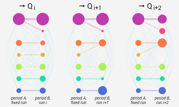
Figure 2: Choosing the best combination. Given a set of clusters from period A, we perform the matching algorithm between these clusters and N=100 sets of clusters from period B obtained by independent runs of the Louvain algorithm. In each case, we compute the modularity $Q$ obtained by grouping paired clusters in a single clusters in the 2-periods BC network. The ‘best combination’ is defined as the set of clusters from period B maximizing this quantity.

2.4 BiblioTools / BiblioMaps

All the data sets were extracted from the ISI Web of Knowledge Core Collection database. The bibliographic records were parsed and analyzed using Bibliotools, a Python-based open-source software and the historical streams figures were generated using the web-based visualisation platform BiblioMaps Grauwin & Jensen (2011); Lund et al. (2017); Grauwin & Sperano (2018). Bibliotools and its extension BiblioMaps were developed by one of us and are available online, as all the data analysis presented in this paper.

2.5 Normalized Mutual Information

The mutual information (MI) is a widely used measure for comparing community detection algorithms. It is defined as a measure of the statistical independence between two random variables (see eq. 2). In other words, if $H(P_{X})$ is the entropy associated with partition $X$ and $H(P_{Y})$ is the entropy associated with partition $Y$ (the entropy is a measure of how partitioned is our network, the more communities - here temporal streams - the higher the entropy), then $MI(P_{X},P_{Y})$ represents the overlap of the two partitions. In layman’s terms, it tells us how much we know about the partition $P_{X}$ when the partition $P_{Y}$ is given. You may refer to Wagner & Wagner (2007); Kvålseth (2017) for a deeper description on mutual information. In particular, note that the mutual information is a symmetrical measure

$$MI(P_{X},P_{Y})=H(P_{Y})-H(P_{Y}|P_{X})=MI(P_{Y},P_{X})$$ (2)

The MI is defined on $[0,+\infty]$, therefore it is difficult to make sense of it without an upper-bound. There exists different ways to normalize the mutual information. The idea is to take into account the entropies of the partitions we consider to gauge the proportion of mutual information between the partitions. Normalizing by the entropy of one of the partition, e.g. $H(P_{X})$ (see eq. 3) measures how much of the partition $P_{X}$ is included in the partition $P_{Y}$. We call this normalized mutual information $NMI_{X}$. If it reaches its maximum value 1, it means that it is possible to retrieve all the information (the partition) of $P_{X}$ from the partition $P_{Y}$. However this measure does not take into account the size of the other partition, $P_{Y}$. A partition $P_{Y}$ where each node would be its own community would make $NMI_{X}$ equals to 1 even though both partitions are very different. This measure then needs to be combined with at least another NMI which takes into account the relative size of both partitions (see eq. 4). Here the mutual information is normalized by $\sqrt{H(P_{X})*H(P_{Y})}$, which shows how much of the two entropies overlap on a scale between 0 and 1. This expresses how similar the partitions are. It is equal to 1 when the partitions are the same. Moreover, this last NMI is symmetrical, so it takes into account both retrieval of $P_{X}$ from $P_{Y}$ and retrieval of $P_{Y}$ from $P_{X}$.

$$NMI_{X}(P_{X},P_{Y})=\frac{MI(P_{X},P_{Y})}{H(P_{X})}$$ (3)

$$NMI(P_{X},P_{Y})=\frac{MI(P_{X},P_{Y})}{\sqrt{H(P_{X})*H(P_{Y})}}=NMI(P_{Y},P_{X})$$ (4)

While Mutual information based measures give a value of similarity between two partitions, it is not straightforward to analyze. For example, it does not allow to track where the (dis)similarities come from. To allow in depth comparison, we represent pairs of partitions as bipartite networks.

2.6 Bipartite Network of streams

To track and quantify differences between partitions $X$ and $Y$, we compute a bipartite network where the $n_{X}^{i}\in N_{X}$ are the first kind of nodes. They represent the streams $s_{X}^{i}\in P_{X}$ (hence $|N_{X}|=|P_{X}|$). It follows that the second kind of nodes $n_{Y}^{j}\in N_{Y}$ represent the streams $s_{Y}^{j}\in P_{Y}$. A weighted directed edge is drawn between $n_{X}^{i}$ and $n_{Y}^{j}$ only if their corresponding streams $s_{GA}^{i}$ and $s_{BCLC}^{j}$ share articles. For a given pair of nodes ($n_{X}^{i}$,$n_{Y}^{j}$) the weights of the two edges between them (one in each direction) are defined in eq.5. We quantify differences between streams of two partitions from this graph, quantities are given in table 3.

$$\left\{\begin{aligned} w_{n_{X}^{i}\rightarrow n_{Y}^{j}}=\frac{|s_{X}^{i}\cap s_{Y}^{j}|}{|s_{X}^{i}|}\\ w_{n_{Y}^{j}\rightarrow n_{X}^{i}}=\frac{|s_{Y}^{j}\cap s_{X}^{i}|}{|s_{Y}^{j}|}\end{aligned}\right.$$ (5)

3 Data sets

In this section, we present the specificity of each data set and the motivations for studying them. Key statistical data are summarized in table 1.

data set	Type	Period	N	$N_{BC}$	$\rho_{links}$	$<d>$	$<w>$	$Q_{GA}$
Wavelets	Thematic	1963-2012	6,582	5,568	0.0065	35.98	0.000719	0.677
ENS-Lyon	Institution	1988-2017	16,679	14,389	0.0019	27.04	0.000175	0.919

Table 1: Statistics on data sets investigated in the paper. Type is the type of organization data come from. Period is the period over which spans the data set. N is the number of publications in the data set. $N_{BC}$ is the number of articles in the BC table. $\rho_{links}$ is the density of links in the BC network. $<d>=(N_{BC}-1)*\rho_{links}$, it indicates the average number of publications a given publication shares references with. $<w>$ indicates the average link weight. Q is the modularity of the network using global partitioning (GA).

3.1 ENS-Lyon Publications data set

The ENS-Lyon Publications data set contains all publications produced by researchers affiliated to the École Normale Supérieure de Lyon in natural science fields. It spans the 1988-2017 period and contains 16,679 publications. As for many scientific institutions, its publication records is highly structured by disciplinary academic departments. Here, we compare our temporal clustering methods to a partition that clusters articles according to their authors’ laboratories (reference partition, $P_{REF}$).

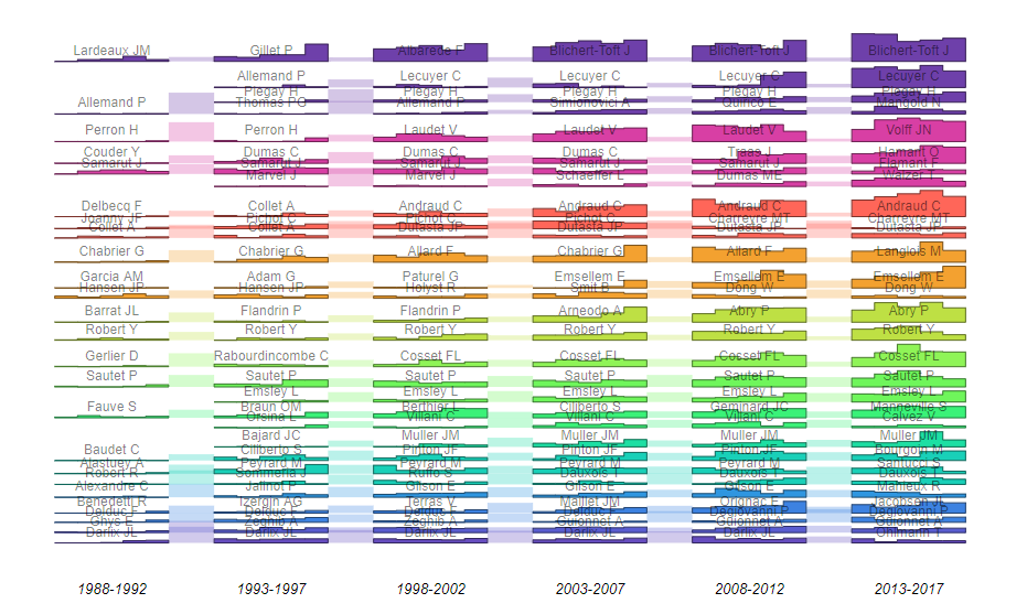
(a) Historical streams computed from the ENS Lyon natural sciences publications. Streams were determined using the global algorithm (GA).

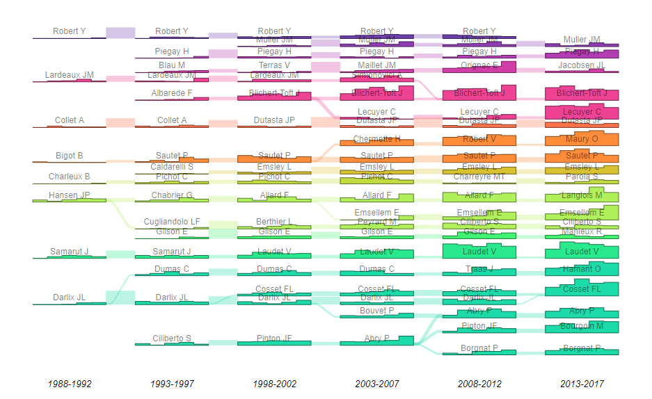
(a) Historical streams computed from the ENS Lyon natural sciences publications. Streams were computed using our local method (BCLC).

Figure 4: Labels on each stream correspond to the most frequent author name in that stream during a given period. Streams with the same color have close research topics (here the proximity of streams to each other is computed from the weight of BC network links between clusters of a same period). Bar height is proportional to the number of publications in a given year. Links between streams show the streams that are preceding/following each other.

3.2 Wavelets Publications data set

The Wavelets Publications data set contains all publications related to wavelets and spans from 1910 to 2012 (however the period before 1960 contains only a few publications). This data set contains 6,582 publications, corresponding to all the publications of a list of 83 key actors in the field of wavelets selected by expert advice and bibliographic searches (for more details, see Morini et al. (2017)). The study of this data set represents a difficult task because it emerged from the collaboration of several research fields, constituted by many entangled subfields. Based on the knowledge of one of the authors (PF), a field’s expert, we built manually a temporal partition drawing the history of wavelets. We refer to this partition as $P_{REF}$ and compare our automatically generated partitions to this partition of reference. We acknowledge that this partition is not an absolute ground truth as it relies on the subjectivity of an expert. However, we assume that this reference gives a reasonable picture of the field’s evolution.

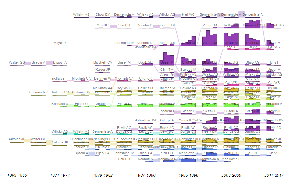
(a) Historical streams computed from the wavelets field of research publications. Streams determined using the global algorithm (GA).

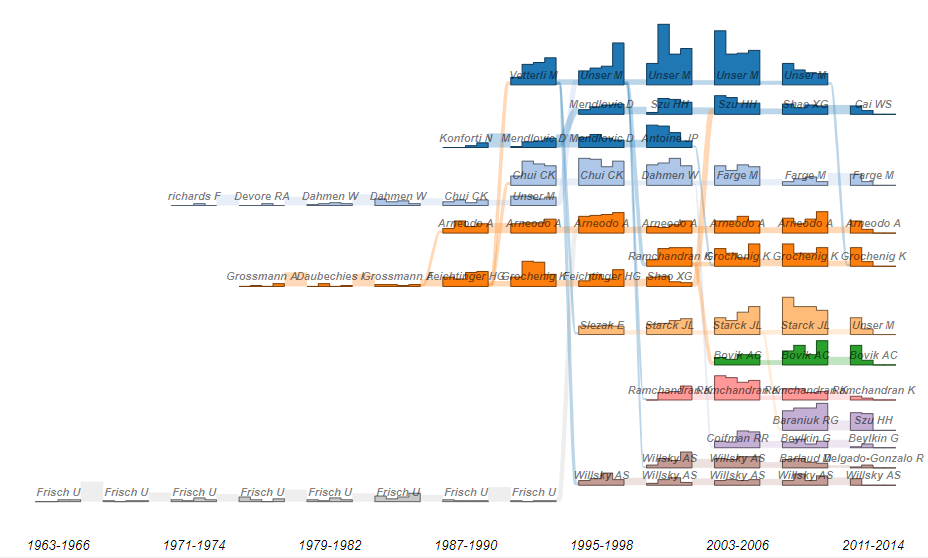
(a) Historical streams computed from the wavelets field of research publications. Streams were computed using our local method (BCLC).

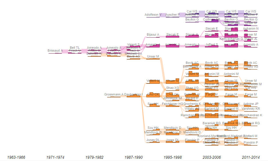
(a) Historical streams computed from the wavelets field of research publications. Streams are the reference streams determined manually.

Figure 7: Labels on each stream correspond to the most frequent author name in that stream during a given period. Streams with the same color have close research topics (here the proximity of streams to each other is computed from the weight of BC network links between clusters of a same period). Bar height is proportional to the number of publications in a given year. Links between streams show the streams that are preceding/following each other.

4 Results

It is difficult to represent the richness of the information conveyed by streams in paper figures. To be able to attribute scientific meaning to each of the streams, and characterize them through their main authors, references, keywords… an interactive stream visualization is available at http://www.sebastian-grauwin.com/streams/BCstreams.html.

4.1 General features

As illustrated in Figures 4 and 7, the global method cannot lead to a rich dynamics description. By construction, GA streams are well separated from each other (Figure 3(a)) and show only a few links in Figure 5(a), which could be interpreted as splits or merges of subfields. On the opposite, BCLC streams lead to a more dynamical history for both data sets. There are only a few links Figure 4(a), because different streams correspond to different scientific (sub)disciplines, which are known to be only marginally connected. However, our method rightly spots teams that split to focus on different research topics (as streams ‘Blichert-Toft’ and ‘Lecuyer’, 6^th and 7^th from the top). Similarly, many splits and merges occur in Figure 6(a). To analyze these differences, we compare the partitions for each data set using the two measures defined above : Mutual information (table 2) and community similarity from the bipartite network representation.

Measures	ENS-Lyon	Wavelets
$|P_{GA}|$	57	27
$|P_{BCLC}|$	97	36
$|P_{REF}|$	17	36
$H(P_{GA})$	3.63	2.87
$H(P_{BCLC})$	4.05	3.04
$H(P_{REF})$	2.37	3.18
$MI(GA,REF)$	1.93	2.03
$MI(BCLC,REF)$	1.93	2.49
$MI(GA,BCLC)$	3.10	1.90
$NMI_{REF}(GA,REF)$	0.82	0.64
$NMI_{REF}(BCLC,REF)$	0.81	0.80
$NMI(GA,BCLC)$	0.81	0.64

Table 2: $|P_{X}|$ is the number of streams in partition $X$. $H(P_{X})$ is the entropy of partition $X$. $MI(P_{X},P_{Y})$ is the mutual information between the partitions $X$ and $Y$. $NMI_{REF}$ is the mutual information MI normalized by $H(P_{REF})$. $NMI(GA,BCLC)$ is the symmetrical normalized mutual information (normalized by $\sqrt{H(GA)*H(BCLC)}$).

4.2 Results on ENS Lyon data set

Table 2 shows the highly different number of streams of each partition : 57 streams for the global method, 97 for the local one and only 17 for the reference partition (the 17 laboratories of the ENS Lyon). The high values of $NMI_{REF}(GA,REF)$ (0.82) and $NMI_{REF}(BCLC,REF)$ (0.81) suggest that the extra streams in both $P_{GA}$ and $P_{BCLC}$ are mostly hierarchical subdivisions of the laboratory streams from $P_{REF}$. A partition being a subdivision of another does not result in a decrease of MI between them. The MI decreases only if communities of a partition need to be mixed to become communities of another. These results suggest that $P_{GA}$ and $P_{BCLC}$ are merely a smaller-scale division of $P_{REF}$. Similarly, the high value of $NMI(GA,BCLC)$ (0.81) suggests that $P_{BCLC}$ and $P_{GA}$ convey the same information.

The measures from Table 3 confirm this analysis. $\overline{1^{st}E}(GA,REF)$ shows that streams from $P_{GA}$ share on average $86\pm 17\%$ of their articles with a stream from $P_{REF}$ and an average of $3.37\pm 1.76$ streams from $P_{GA}$ are needed to retrieve 80% of streams from $P_{REF}$. Similar observations can be made for $P_{BCLC}$. Moreover, $\overline{Sum_{80}}(GA,BCLC)$ shows that it takes on average two streams from $P_{BCLC}$ to reach 80% of streams from $P_{GA}$.

Figure 8 shows a part of the bipartite network between $P_{GA}$ (left) and $P_{BCLC}$ (right) on the ENS Lyon publications data set. The part of the network is centered on nine streams from $P_{GA}$ equivalent to 17 streams from $P_{BCLC}$. It suggests that streams from $P_{REF}$ are not a mix of different streams from $P_{GA}$ or $P_{BCLC}$. They are rather unions of (almost) entire streams, which means that GA and BCLC yield almost the same partitions, but at different scales.

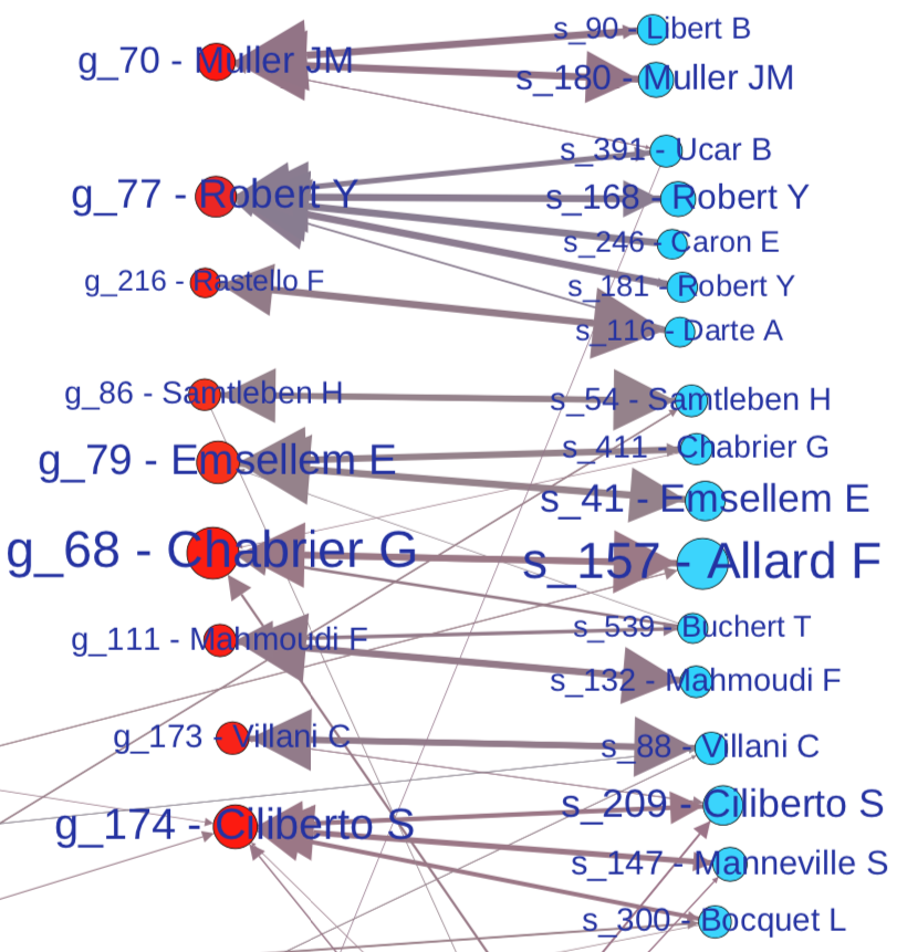
Figure 8: Part of the bipartite network representation of ENS Lyon data set. This network shows the links between temporal communities from $P_{GA}$ (left in red) and $P_{BCLC}$ (right in blue). On each node is given the stream ID and the most frequent author name of the temporal community. Size of nodes accounts for the size of the streams, each stream contains at least 20 articles.

4.3 Results on Wavelets data set

4.3.1 Overall comparison

Describing the history of the wavelets research field is a complicated task as it was born from the collaboration of multiple fields and sub-fields. The values from table 2 show that, even though partitions have a similar number of streams (27 for $P_{GA}$ and 36 for $P_{BCLC}$), there are significant differences between the local and global method. In this case, $NMI(BCLC,REF)$ is significantly higher than $NMI(GA,REF)$ (0.82 vs. 0.68). Moreover $NMI(GA,BCLC)$ is rather low (0.64) which suggests that differences do not only arise from differences of scale. We visualize some of these differences in section 4.3.2. From Table 3 we see that most similar streams between $P_{GA}$ and $P_{REF}$ share $75\%\pm 20\%$ of articles on average, whereas the corresponding figure for $P_{BCLC}$ and $P_{REF}$ is $87\%\pm 17\%$.

Measures	ENS-Lyon	Wavelets
$\overline{1^{st}E}(GA,REF)$	$0.86\pm 0.17$	$0.75\pm 0.20$
	$0.49\pm 0.20$	$0.81\pm 0.17$
$\overline{Sum_{80}}(GA,REF)$	$1.26\pm 0.54$	$1.88\pm 0.93$
	$3.37\pm 1.76$	$1.5\pm 0.73$
$\overline{1^{st}E}(BCLC,REF)$	$0.89\pm 0.14$	$0.87\pm 0.17$
	$0.49\pm 0.26$	$0.87\pm 0.15$
$\overline{Sum_{80}}(BCLC,REF)$	$1.23\pm 0.44$	$1.26\pm 0.50$
	$4.87\pm 3.35$	$1.31\pm 0.57$
$\overline{1^{st}E}(GA,BCLC)$	$0.74\pm 0.23$	$0.72\pm 0.23$
	$0.85\pm 0.16$	$0.83\pm 0.19$
$\overline{Sum_{80}}(GA,BCLC)$	$1.96\pm 1.14$	$1.88\pm 0.96$
	$1.34\pm 0.51$	$1.61\pm 0.83$

Table 3: In this table each cell contains two lines. Each measure $M(X,Y)$ is made on edges. The first line correspond to $M$ measured on edges from $n_{X}$ to $n_{Y}$ and the second line corresponds to $M$ being measured on edges from $n_{Y}$ to $n_{X}$. So, the first row in $\overline{1^{st}E}(X,Y)$ is the average proportion of articles $n_{X}$ shares with $n_{Y}$ $\pm$ its standard deviation. The second row is the average proportion of articles $n_{Y}$ shares with $n_{X}$ $\pm$ its standard deviation. For instance, for the ENS-Lyon, this means that streams of $P_{GA}$ share on average 86% of their articles with their most similar stream in $P_{REF}$, whereas streams from $P_{REF}$ only share on average 49% of their articles with their most similar stream in $P_{GA}$. $\overline{Sum_{80}}(X,Y)$ is the average number of streams from $P_{Y}$ it takes to retrieve 80% of the streams’ articles from $P_{X}$. For example in the case of the Wavelet data set, on average $1.88\pm 0.96$ streams from $P_{BCLC}$ are needed to retrieve 80% of a stream from $P_{GA}$.

4.3.2 Examples of major differences

We now show some major differences between $P_{GA}$ and $P_{BCLC}$ for the wavelets data set. From Figure 9, we can see two types of differences between partitions: scale differences (e.g. g_9 with s_51 and s_166) as in the ENS Lyon case; and more significant differences, when fractions of $P_{GA}$ streams have to be combined to retrieve $P_{BCLC}$ streams (for example, the group of streams around g_5 and g_10). Interestingly, g_7 combines scale and mixing differences. Looking at the BN representation of these $P_{BCLC}$ streams with corresponding $P_{REF}$ streams (Figure 10), we see that our $P_{BCLC}$ description is quite similar to the reference description. There are more ‘stream-to-stream’ equivalences, represented by the double arrow on each side of the edge linking streams. Note that, though $P_{BCLC}$ is closer to $P_{REF}$, there are still scale differences (e.g. s_21, s_111) and mixing differences (e.g. s_85, s_52).

To understand the origin of the better match of $P_{BCLC}$ to the reference, it is instructive to inspect some of the differences between the local ($P_{BCLC}$) and the global partition $P_{GA}$. Let’s look first at the difference between the global method stream g_7, which corresponds to a merger of four local streams, among which s_21 and s_53 (see Fig. 9). Figure 6(a) shows that these streams do not belong to the same time period. Stream s_53 corresponds to the bottom stream (labelled ’Frisch’), and represents early works on wavelets, from 1963 to 1994, focusing on multi fractal analysis and turbulence. The second stream, s_21 (1987 - 2014, 6th from the top, labelled ’Arneodo’), addressed similar issues in a first period and then, since the early 90’s, enlarged the subject matter to include mathematical formalization, together with new applications beyond turbulence, such as genome characterization. Our method appropriately distinguishes these two streams, which correspond to different subfields. The second difference relates to the evolution of one of the authors’ (PF) activities. In the global approach, most PF articles belong to a single cluster that gathers papers in signal representations, and especially time-frequency representations that have been at the heart of his works over the years (third stream starting from the bottom in Fig5(a)). This is a good approximation, but a finer description of the subjects addressed by PF during his career include three topics: (a) time-frequency methods per se, (b) relations of these methods with wavelets and (c) wavelet methods related to self-similarity, in domains such as turbulence. Using the interactive stream visualization, it is possible to look for $BCLC$ streams containing PF’s publications. One finds three streams, addressing the three topics described above, and corresponding to (the stream label refers to its position in Fig6(a), starting from the top) respectively streams 3, 8 and 6. These two examples suggest that $BCLC$ is able to capture the complexity of a field dynamics’, including relevant subfields, while the global approach tends to merge streams that represent different fields of inquiry.

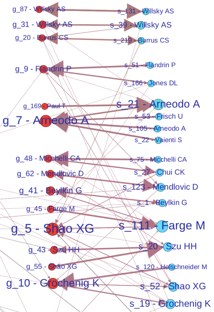
Figure 9: Part of the bipartite network representation of Wavelets data set. This network shows the links between temporal communities from $P_{GA}$ (left in red) and $P_{BCLC}$ (right in blue). Each node is labelled by the stream ID and the most frequent author name of the temporal community. Node size accounts for stream size.

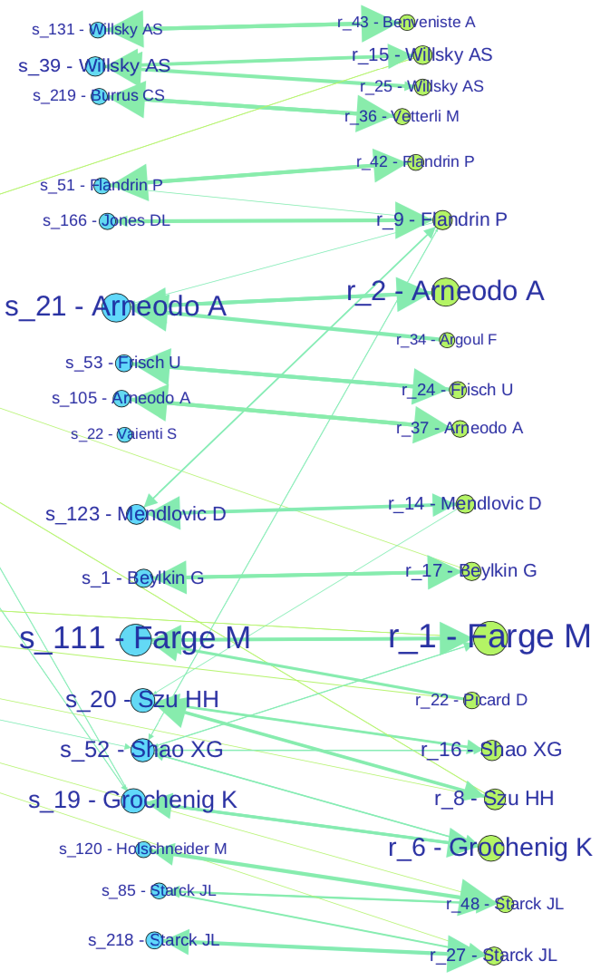
Figure 10: Part of the bipartite network representation of Wavelets data set. This network shows the links between temporal communities from $P_{BCLC}$ (left in blue) and $P_{REF}$ (right in green). Each node is labelled by the stream ID and the most frequent author name of the temporal community. Node size accounts for stream size.

5 Discussion

We have presented a coherent approach to create a dynamic mesoscopic description of a temporal network. As the standard method to used to create static communities, our method only uses modularity to build the dynamic communities. We have compared our method to the static (global) approach. We first showed that both methods give the same result for networks with well-separated streams (high modularity), as in the case of ENS-Lyon publications. However, when analyzing data sets with more complex dynamics, as for the birth of wavelets (section 4.3.2), our method can generate a more satisfactory dynamics, as compared to an expert reference partition.

Clearly, much more work is needed to develop a standard approach for describing dynamical networks at a mesoscopic scale. The stochastic character of many partitioning algorithms (as Louvain’s Blondel et al. (2008)), and the different scales generated by each method make comparisons difficult. Moreover, the dynamical character of the communities renders the definition of an acceptable reference partition even trickier than for static networks.

Appendix A Dynamics of Scientific Research Communities

We investigated four temporal community detection methods, two global and two local methods. However, as measures from GA and GPA are very close and measures from BMLA and BCLC are also very close, we only presented the GA and BCLC methods in the core of this article. The two other methods (GPA and BMLA) and their measures are described below.

A.1 Global Projected Algorithm (GPA)

Here, we want to include some dynamics into our global algorithm. We thus start with the set of GA-streams obtained by running the Louvain algorithm Blondel et al. (2008) on the global BC network. Then, we define BC networks in each period, only keeping the articles sharing at least two references with at least one other article within the period. Removing the “long-term connections only” articles which do not share two or more references with another article in their period results in an average loss of 7.8% of the articles taken into account in the global BC network. For each time period, we define local communities by grouping together the publications that are in the same GA-streams, resulting in a set of local projected communities in each period. Finally, we compute historical streams by applying our matching algorithm to the projected communities. Interestingly, the streams that are build from this method do not necessarily correspond to the GA-streams: the predecessors / successors of a cluster may not be subsets of the same GA-stream of this particular cluster, resulting in splits or merges. In practice, a few GA-streams may in effect be cut into into two or more GPA-streams localized in different time periods. This approach thus allows to visualize the evolution of a GA-stream in terms of dynamical events (splits and merges).

A.2 Best-Modularity Local Algorithm (BMLA)

For each time period, we run $N$ independent runs (we used $N=100$) of the Louvain algorithm. Because of the noise inherent to the Louvain algorithm, these partitions may be a bit different, while having similar modularity values (in practice the modularity difference between the partitions of different runs is lower than 0.005). Compared to the BCLC method, we do not try here to choose the partitions of the run best matching the partition from the previous or next period, but keep the partition with the best modularity among the $N$ runs in each time period. BMLA historical streams are then defined by applying the matching algorithm to these ‘best-modularity’ partitions.

BMLA Algorithm

Compute the Bibliographic Coupling Graph ;

Split the data set into temporal windows $\Delta t$ ;

for each temporal window do

       run $N=100$ Louvain algorithm on the instant network;

       select the instant partition with the highest modularity $Q$;

      

end for

Match the most similar communities between successive temporal windows ;

Link the paired communities along time;

 

This algorithm returns temporal streams we call BMLA-streams. These streams maximize the modularity at each time $t$ without considering the global modularity of the whole system.

A.3 Comparing All Algorithms

Measures	ENS-Lyon	Wavelets
$|P_{GA}|$	57	27
$|P_{GPA}|$	54	30
$|P_{BCLC}|$	97	36
$|P_{BMLA}|$	103	40
$|P_{REF}|$	17	36
$H(P_{GA})$	3.63	2.87
$H(P_{GPA})$	3.63	2.94
$H(P_{BCLC})$	4.05	3.04
$H(P_{BMLA})$	4.04	3.17
$H(P_{REF})$	2.37	3.18
$MI(GA,REF)$	1.93	2.03
$MI(GPA,REF)$	1.94	2.09
$MI(BCLC,REF)$	1.93	2.49
$MI(BMLA,REF)$	1.94	2.47
$MI(GA,BCLC)$	3.10	1.90
$NMI_{GA}(GA,REF)$	0.53	0.73
$NMI_{REF}(GA,REF)$	0.82	0.64
$NMI(GA,REF)$	0.66	0.68
$NMI_{GPA}(GPA,REF)$	0.54	0.74
$NMI_{REF}(GPA,REF)$	0.82	0.66
$NMI(GPA,REF)$	0.67	0.70
$NMI_{BCLC}(BCLC,REF)$	0.48	0.84
$NMI_{REF}(BCLC,REF)$	0.81	0.80
$NMI(BCLC,REF)$	0.63	0.82
$NMI_{BMLA}(BMLA,REF)$	0.48	0.78
$NMI_{REF}(BMLA,REF)$	0.82	0.80
$NMI(BMLA,REF)$	0.63	0.79
$NMI_{GA}(GA,BCLC)$	0.86	0.67
$NMI_{BCLC}(GA,BCLC)$	0.77	0.62
$NMI(GA,BCLC)$	0.81	0.64

Table 4: Similarly to Table 2, $|P_{X}|$ is the number of streams in partition $X$. $H(P_{X})$ is the entropy of partition $X$. $MI(P_{X},P_{Y})$ is the mutual information between the partitions $X$ and $Y$. $NMI_{X}$ is the mutual information MI normalized by $H(P_{X})$. $NMI(P_{X},P_{Y})$ is the symmetrical normalized mutual information (normalized by $\sqrt{H(X)*H(Y)}$).

Measures	ENS-Lyon	Wavelets
$\overline{1^{st}E}(GA,REF)$	$0.86\pm 0.17$	$0.75\pm 0.20$
	$0.49\pm 0.20$	$0.81\pm 0.17$
$\overline{Sum_{80}}(GA,REF)$	$1.26\pm 0.54$	$1.88\pm 0.93$
	$3.37\pm 1.76$	$1.5\pm 0.73$
$\overline{1^{st}E}(GPA,REF)$	$0.87\pm 0.16$	$0.78\pm 0.19$
	$0.54\pm 0.23$	$0.83\pm 0.17$
$\overline{Sum_{80}}(GPA,REF)$	$1.24\pm 0.5$	$1.65\pm 0.84$
	$3.12\pm 1.61$	$1.47\pm 0.72$
$\overline{1^{st}E}(BCLC,REF)$	$0.89\pm 0.14$	$0.87\pm 0.17$
	$0.49\pm 0.26$	$0.87\pm 0.15$
$\overline{Sum_{80}}(BCLC,REF)$	$1.23\pm 0.44$	$1.26\pm 0.50$
	$4.87\pm 3.35$	$1.31\pm 0.57$
$\overline{1^{st}E}(BMLA,REF)$	$0.89\pm 0.14$	$0.85\pm 0.19$
	$0.49\pm 0.25$	$0.84\pm 0.17$
$\overline{Sum_{80}}(BMLA,REF)$	$1.23\pm 0.44$	$1.34\pm 0.63$
	$5.0\pm 3.60$	$1.37\pm 0.59$
$\overline{1^{st}E}(GA,BCLC)$	$0.74\pm 0.23$	$0.72\pm 0.23$
	$0.85\pm 0.16$	$0.83\pm 0.19$
$\overline{Sum_{80}}(GA,BCLC)$	$1.96\pm 1.14$	$1.88\pm 0.96$
	$1.34\pm 0.51$	$1.61\pm 0.83$

Table 5: Similarly to Table 3, In this table each cell contains two lines. Each measure $M(X,Y)$ is made on edges. The first line correspond to $M$ measured on edges from $n_{X}$ to $n_{Y}$ and the second line corresponds to $M$ being measured on edges from $n_{Y}$ to $n_{X}$. So, the first row in $\overline{1^{st}E}(X,Y)$ is the average proportion of articles $n_{X}$ shares with $n_{Y}$ $\pm$ its standard deviation. The second row is the average proportion of articles $n_{Y}$ shares with $n_{X}$ $\pm$ its standard deviation. For instance, for the ENS-Lyon, this means that streams of $P_{GA}$ share on average 86% of their articles with their most similar stream in $P_{REF}$, whereas streams from $P_{REF}$ only share on average 49% of their articles with their most similar stream in $P_{GA}$. $\overline{Sum_{80}}(X,Y)$ is the average number of streams from $P_{Y}$ it takes to retrieve 80% of the streams’ articles from $P_{X}$. For example in the case of the Wavelet data set, on average $1.88\pm 0.96$ streams from $P_{BCLC}$ are needed to retrieve 80% of a stream from $P_{GA}$.

Table 4 and Table 5 show there is very little difference between the local algorithms and between the global algorithms, for all measures on both data sets.

References

- (1)
- Aynaud et al. (2013) Aynaud, T., Fleury, E., Guillaume, J.-L. & Wang, Q. (2013), Communities in evolving networks: Definitions, detection, and analysis techniques, in A. Mukherjee, M. Choudhury, F. Peruani, N. Ganguly & B. Mitra, eds, ‘Dynamics On and Of Complex Networks, Volume 2: Applications to Time-Varying Dynamical Systems’, Springer New York, New York, NY, pp. 159–200.
-
Barthélemy (2011)
Barthélemy, M. (2011), ‘Spatial networks’,
Physics Reports 499(1), 1 – 101.
http://www.sciencedirect.com/science/article/pii/S037015731000308X -
Blondel et al. (2008)
Blondel, V. D., Guillaume, J.-L., Lambiotte, R. & Lefebvre, E.
(2008), ‘Fast unfolding of communities in
large networks’, Journal of Statistical Mechanics: Theory and
Experiment 2008(10), P10008.
http://stacks.iop.org/1742-5468/2008/i=10/a=P10008 -
Boccaletti et al. (2006)
Boccaletti, S., Latora, V., Moreno, Y., Chavez, M. & Hwang, D.-U.
(2006), ‘Complex networks: Structure and
dynamics’, Physics Reports 424(4), 175 – 308.
http://www.sciencedirect.com/science/article/pii/S037015730500462X -
Claveau & Gingras (2016)
Claveau, F. & Gingras, Y. (2016),
‘Macrodynamics of Economics: A Bibliometric History’, History of
Political Economy 48(4), 551–592.
https://doi.org/10.1215/00182702-3687259 -
Dall’Asta et al. (2006)
Dall’Asta, L., Barrat, A., Barthélemy, M. & Vespignani, A.
(2006), ‘Vulnerability of weighted
networks’, Journal of Statistical Mechanics: Theory and Experiment 2006(04), P04006.
http://stacks.iop.org/1742-5468/2006/i=04/a=P04006 -
Duan et al. (2009)
Duan, D., Li, Y., Jin, Y. & Lu, Z. (2009), Community mining on dynamic weighted directed graphs,
in ‘Proceedings of the 1st ACM International Workshop on Complex
Networks Meet Information & Knowledge Management’, CNIKM ’09, ACM, New
York, NY, USA, pp. 11–18.
http://doi.acm.org/10.1145/1651274.1651278 -
Fortunato & Barthélemy (2007)
Fortunato, S. & Barthélemy, M. (2007), ‘Resolution limit in community detection’, Proceedings of the National Academy of Sciences 104(1), 36–41.
http://www.pnas.org/content/104/1/36 -
Fortunato & Hric (2016)
Fortunato, S. & Hric, D. (2016),
‘Community detection in networks: A user guide’, Physics Reports 659, 1 – 44.
Community detection in networks: A user guide.
http://www.sciencedirect.com/science/article/pii/S0370157316302964 -
Ghasemian et al. (2016)
Ghasemian, A., Zhang, P., Clauset, A., Moore, C. & Peel, L.
(2016), ‘Detectability thresholds and
optimal algorithms for community structure in dynamic networks’, Phys.
Rev. X 6, 031005.
https://link.aps.org/doi/10.1103/PhysRevX.6.031005 -
Görke et al. (2013)
Görke, R., Maillard, P., Schumm, A., Staudt, C. & Wagner, D.
(2013), ‘Dynamic graph clustering combining
modularity and smoothness’, J. Exp. Algorithmics 18, 1.5:1.1–1.5:1.29.
http://doi.acm.org/10.1145/2444016.2444021 - Görke et al. (2010) Görke, R., Maillard, P., Staudt, C. & Wagner, D. (2010), Modularity-driven clustering of dynamic graphs, in P. Festa, ed., ‘Experimental Algorithms’, Springer Berlin Heidelberg, Berlin, Heidelberg, pp. 436–448.
-
Grauwin & Jensen (2011)
Grauwin, S. & Jensen, P. (2011),
‘Mapping scientific institutions’, Scientometrics 89(3), 943.
https://doi.org/10.1007/s11192-011-0482-y - Grauwin & Sperano (2018) Grauwin, S. & Sperano, I. (2018), ‘Bibliomaps-a software to create web-based interactive maps of science: The case of ux map’, Proceedings of the Association for Information Science and Technology 55(1), 815–816.
- Greene et al. (2010) Greene, D., Doyle, D. & Cunningham, P. (2010), Tracking the evolution of communities in dynamic social networks, in ‘2010 International Conference on Advances in Social Networks Analysis and Mining’, pp. 176–183.
-
Guo et al. (2014)
Guo, C., Wang, J. & Zhang, Z. (2014), ‘Evolutionary community structure discovery in
dynamic weighted networks’, Physica A: Statistical Mechanics and its
Applications 413, 565 – 576.
http://www.sciencedirect.com/science/article/pii/S037843711400569X - Hartmann et al. (2016) Hartmann, T., Kappes, A. & Wagner, D. (2016), Clustering evolving networks, in L. Kliemann & P. Sanders, eds, ‘Algorithm Engineering: Selected Results and Surveys’, Springer International Publishing, Cham, pp. 280–329.
-
Holme (2015)
Holme, P. (2015), ‘Modern temporal network
theory: a colloquium’, The European Physical Journal B 88(9), 234.
https://doi.org/10.1140/epjb/e2015-60657-4 -
Holme & Saramäki (2012)
Holme, P. & Saramäki, J. (2012), ‘Temporal networks’, Physics Reports 519(3), 97 – 125.
Temporal Networks.
http://www.sciencedirect.com/science/article/pii/S0370157312000841 -
Kvålseth (2017)
Kvålseth, T. O. (2017), ‘On normalized
mutual information: Measure derivations and properties’, Entropy 19(11), 631.
http://www.mdpi.com/1099-4300/19/11/631 -
Lariviere et al. (2008)
Lariviere, V., Archambault, E. & Gingras, Y. (2008), ‘Long-term variations in the aging of scientific
literature: From exponential growth to steady-state science (1900–2004)’,
Journal of the American Society for Information Science and Technology
59(2), 288–296.
https://onlinelibrary.wiley.com/doi/abs/10.1002/asi.20744 - Lorenz et al. (2018) Lorenz, P., Wolf, F., Braun, J., Djurdjevac Conrad, N. & Hövel, P. (2018), Capturing the dynamics of hashtag-communities, in C. Cherifi, H. Cherifi, M. Karsai & M. Musolesi, eds, ‘Complex Networks & Their Applications VI’, Springer International Publishing, Cham, pp. 401–413.
- Lund et al. (2017) Lund, K., Jeong, H., Grauwin, S. & Jensen, P. (2017), ‘Une carte scientométrique de la recherche en éducation vue par la base de données internationales scopus’, Les Sciences de l’education-Pour l’Ere nouvelle 50(1), 67–84.
-
Masuda & Lambiotte (2016)
Masuda, N. & Lambiotte, R. (2016),
A Guide to Temporal Networks, WORLD SCIENTIFIC (EUROPE).
https://www.worldscientific.com/doi/abs/10.1142/q0033 -
Matias & Miele (2016)
Matias, C. & Miele, V. (2016),
‘Statistical clustering of temporal networks through a dynamic stochastic
block model’, Journal of the Royal Statistical Society: Series B
(Statistical Methodology) 79(4), 1119–1141.
https://rss.onlinelibrary.wiley.com/doi/abs/10.1111/rssb.12200 -
Morini et al. (2017)
Morini, M., Flandrin, P., Fleury, E., Venturini, T. & Jensen, P.
(2017), Revealing evolutions in dynamical
networks.
working paper or preprint.
https://hal.inria.fr/hal-01558219 -
Mucha et al. (2010)
Mucha, P. J., Richardson, T., Macon, K., Porter, M. A. & Onnela,
J.-P. (2010), ‘Community structure in
time-dependent, multiscale, and multiplex networks’, Science 328(5980), 876–878.
http://science.sciencemag.org/content/328/5980/876 -
Newman (2003)
Newman, M. (2003), ‘The structure and
function of complex networks’, SIAM Review 45(2), 167–256.
https://doi.org/10.1137/S003614450342480 -
Newman (2006)
Newman, M. E. J. (2006), ‘Modularity and
community structure in networks’, Proceedings of the National Academy of
Sciences 103(23), 8577–8582.
http://www.pnas.org/content/103/23/8577 -
Onnela et al. (2007)
Onnela, J.-P., Saramäki, J., Hyvönen, J., Szabó, G., de Menezes, M. A.,
Kaski, K., Barabási, A.-L. & Kertész, J. (2007), ‘Analysis of a large-scale weighted network of
one-to-one human communication’, New Journal of Physics 9(6), 179.
http://stacks.iop.org/1367-2630/9/i=6/a=179 -
Pastor-Satorras & Vespignani (2001)
Pastor-Satorras, R. & Vespignani, A. (2001), ‘Epidemic spreading in scale-free networks’, Phys. Rev. Lett. 86, 3200–3203.
https://link.aps.org/doi/10.1103/PhysRevLett.86.3200 -
Rossetti & Cazabet (2018)
Rossetti, G. & Cazabet, R. (2018),
‘Community discovery in dynamic networks: A survey’, ACM Comput. Surv.
51(2), 35:1–35:37.
http://doi.acm.org/10.1145/3172867 -
Rossetti et al. (2017)
Rossetti, G., Pappalardo, L., Pedreschi, D. & Giannotti, F.
(2017), ‘Tiles: an online algorithm for
community discovery in dynamic social networks’, Machine Learning 106(8), 1213–1241.
https://doi.org/10.1007/s10994-016-5582-8 - Wagner & Wagner (2007) Wagner, S. & Wagner, D. (2007), Comparing clusterings - an overview, Technical Report 4, Karlsruhe.
- Wang et al. (2008) Wang, Y., Wu, B. & Pei, X. (2008), Commtracker: A core-based algorithm of tracking community evolution, in C. Tang, C. X. Ling, X. Zhou, N. J. Cercone & X. Li, eds, ‘Advanced Data Mining and Applications’, Springer Berlin Heidelberg, Berlin, Heidelberg, pp. 229–240.