Atomic forces by quantum Monte Carlo: Application to phonon dispersion calculations

Abstract

We report a successful application of the ab initio quantum Monte Carlo (QMC) framework to a phonon dispersion calculation. A full phonon dispersion of diamond is successfully calculated at the variational Monte Carlo (VMC) level, based on the frozen-phonon technique. The VMC-phonon dispersion is in good agreement with the experimental results, giving renormalized harmonic optical frequencies very close to the experimental values, and improving upon previous density functional theory estimates. Key to success for the QMC approach is the statistical error reduction in the atomic force evaluation. We show that this can be achieved by using well conditioned atomic basis sets and by explicitly removing the basis-set redundancy, which reduces the statistical error of forces by up to two orders of magnitude by combining it with the so-called space-warp transformation algorithm. This leads to affordable and accurate QMC-phonons calculations, which are up to $10^{4}$ times more efficient than a bare force treatment, and paves the way to new applications, particularly in correlated materials, where phonons have been poorly reproduced so far.

The accurate description of phonons in a solid is one of the central research topics in the field of condensed matter physics and materials science for discussing phase stability (i.e., Gibbs-free energy), electron-phonon interaction, and structural phase transitions of materials Martin (2004); Sholl and Steckel (2011). Ab initio phonon calculations based on the Density Functional Theory (DFT) Baroni et al. (2001); Togo and Tanaka (2015) have been successful for many compounds, but they often fail in strongly-correlated materials. For example, DFT calculations severely underestimate the highest frequency of the optical phonons of graphene at the $K$ point Mounet and Marzari (2005); Lazzeri et al. (2008), because the electron-electron correlation is not taken into account with sufficient accuracy. Another example is the elemental cerium, whose phonon dispersions measured by neutron scattering strongly mismatch with the calculated DFT-PBE ones Krisch et al. (2011). Interestingly, such failure was also seen in a high-$T_{c}$ cuprate superconductor Reznik et al. (2008) Some effort has been made to include correlation in phonon calculations in the DFT+U framework Floris et al. (2011) and also within the DMFT framework Leonov et al. (2012, 2014). In both cases, this requires modeling correlations by an empirical parameter, though physically motivated (i.e., the Hubbard $U$). Indeed, a genuine ab initio framework applicable to strongly correlated materials without any empirical parameters remains, so far, a very important theoretical challenge.

The ab initio quantum Monte Carlo (QMC) framework, including variational quantum Monte Carlo (VMC) and the diffusion quantum Monte Carlo (DMC) schemes, is among the state-of-art numerical methods to obtain highly accurate many-body wave functions Foulkes et al. (2001), and cope with the electron correlation more rigorously than DFT. It has been successfully applied to challenging materials that DFT cannot tackle, such as cuprates Marchi et al. (2011), iron-arsenides Casula and Sorella (2013), and graphene Marchi et al. (2011); Sorella et al. (2018). So far, unfortunately, almost all QMC applications are mainly based on energy and its first derivative (i.e., atomic force) calculations. Indeed, it is at present an open problem how to evaluate, with an affordable computational effort, second and higher-order derivatives, which are essential for computing various physical properties.

There are three routes to compute the second derivatives (i.e., $\frac{\partial^{2}E}{\partial{R_{\alpha}}\partial{R_{\beta}}}$), which are needed for evaluating harmonic phonon properties, by ab initio calculations, i.e., $\rm(\hskip 1.79993pti\hskip 1.79993pt)$ potential energy surface (PES) fitting, $\rm(\hskip 0.80002ptii\hskip 0.80002pt)$ finite difference expression based on atomic force evaluations , and $\rm(iii)$ direct evaluation of second derivatives. All of the above attempts have been successful for isolated molecular systems Zen et al. (2012); Luo et al. (2014); Liu et al. (2019); Nakano et al. (2019). On the other hand, for solids, only strategy $\rm(\hskip 1.79993pti\hskip 1.79993pt)$ has been successful so far within the QMC framework. For example, Maezono et al. calculated Raman frequencies of diamond (phonons at $q=\Gamma$ point) Maezono et al. (2007). However, QMC-phonon calculations of solids have been limited to a single high-symmetry $q$-point. To the best of our knowledge, the full ($q$-resolved) phonon dispersion has been unaccessible so far at both VMC and DMC levels.

In this paper, we report a successful phonon dispersion calculation of diamond at the VMC level by adopting strategy $\rm(\hskip 0.80002ptii\hskip 0.80002pt)$ , the so-called frozen phonon technique Togo and Tanaka (2015). The key to success is to reduce the statistical error of atomic forces. We found that removing the nearly linear dependency of the basis set used for the trial wave function parametrization Azadi et al. (2010) dramatically lowers the statistical error of forces. Its decrease reaches the order of $\times$ ${\sim 10^{-2}}$, which corresponds to a speed-up of ${\sim 10^{4}}$ times in a VMC computation. This drastic reduction enables us to construct a dynamical matrix within an affordable computational time, and to eventually apply VMC-phonon calculations to new interesting materials from first principles.

Table 1: The highest harmonic phonon frequencies (THz) of diamond at high-symmetry $q$ points. All phonons are calculated using the experimental lattice parameter. In this table, (P) denotes the interpolated frequencies obtained by Phonopy, (F) denotes the phonon frequency at $\Gamma$ obtained by fitting forces of distorted structures along the Raman mode with a linear function at the VMC level, and (E) denotes the phonon frequency at $\Gamma$ obtained by fitting energies of undistorted and distorted structures along the Raman mode with a quadratic function at the VMC and LRDMC levels. The last column indicates the harmonic frequencies estimated by the raw experimental values: 39.938 THzLiu et al. (2000), 35.299 THzSchwoerer-Böhning et al. (1998), and 37.962 THzKulda et al. (2002) at the $\Gamma$, $X$, and $L$ points, respectively.

$q$	DFT		Previous work		This work				Experiment
	LDA-PZ	GGA-PBE	VMC	DMC	VMC(P)	VMC(F)	VMC(E)	LRDMC(E)	Harmonic (Estimated)
$\Gamma$	38.55	38.82	41.64(9)	41.22(12)	40.65(38)	40.49(4)	40.68(29)	41.52(22)	40.460, 40.349
$X$	35.64	35.87	-	-	36.48(40)	-	-	-	35.476
$L$	37.31	37.47	-	-	38.01(31)	-	-	-	38.242

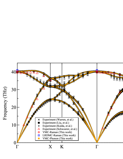
Figure 1: The phonon dispersion and Raman frequencies of diamond calculated using a 2 $\times$ 2 $\times$ 2 conventional supercell at the VMC level, where the anharmonic and one-body finite size corrections are included. The experimental lattice parameter (i.e., 6.741 bohr Parrish (1960)) was employed. The error bars were estimated by the jackknife method. Observed experimental results are also plotted for comparison. Experimental data are taken from Refs. Warren et al., 1965; *1967WAR; Liu et al., 2000; Kulda et al., 2002; Schwoerer-Böhning et al., 1998. The data in Ref. Schwoerer-Böhning et al., 1998 were digitalized using WebPlotDigitizer Rohatgi (2020).

All Variational Monte Carlo (VMC) and lattice regularized diffusion Monte Carlo (LRDMC) Casula et al. (2005); Nakano et al. (2020a) calculations in this study were performed by the TurboRVB  Casula and Sorella (2003); Nakano et al. (2020b) SISSA quantum Monte Carlo package. We employed the Jastrow Slater-determinant(JSD) ansatz, i.e, $\Psi=\Psi_{\text{SD}}\times\exp J,$ where $\Psi_{\text{SD}}$ and $J$ are the Slater determinant and Jastrow terms, respectively. The Slater determinant part is expressed in terms of molecular orbitals $\phi_{k}(\mathbf{r})=\sum_{i=1}^{L}{c_{i,k}{\psi_{i}}(\mathbf{r})}$ expanded in a periodized Gaussian basis set $\{\psi_{i}\}$. The valence triple-zeta (VTZ) basis set accompanying an energy-consistent pseudo potential developed by Burkatzki et al. Burkatzki et al. (2007) was employed for the primitive Gaussian atomic orbitals (Table S-Ifoo ). The coefficients of atomic orbitals (i.e., $c_{i,k}$) were obtained by a DFT calculation with the LDA-PZ exchange-correlation functional Perdew and Zunger (1981) and were left unchanged during the VMC optimization. The Jastrow factor was composed of inhomogeneous one-, two- and three-body contributions ($J={J_{1}}^{inh}+{J_{2}}+{J_{3}}$). foo The variational parameters in the Jastrow terms were optimized by the stochastic reconfiguration Sorella et al. (2007) and/or the modified linear method Umrigar et al. (2007); Nakano et al. (2020b) implemented in TurboRVB. LRDMC calculations were performed by the single-grid scheme Casula et al. (2005) with a lattice space, $a$ = 0.2 bohr.

In this paper, we focus on diamond (Space group: $Fd\bar{3}m$) as a proof of concept for the first example of a VMC-based phonon dispersion calculation. 2 $\times$ 2 $\times$ 2 conventional supercells (256 electrons / 64 carbon atoms in a simulation cell) were used for most calculations, while 3 $\times$ 3 $\times$ 3 conventional supercells (864 electrons / 216 carbon atoms in a simulation cell) were also used for several calculations to investigate the finite size errors. $L$-twist (i.e., $k$ = $\pi$, $\pi$, $\pi$) was employed for alleviating the so-called one-body finite-size effects Maezono et al. (2007); Hennig et al. (2010); Sorella et al. (2011). Dynamical matrices and the corresponding phonon dispersions were calculated based on the frozen-phonon technique implemented in the Phonopy module Togo and Tanaka (2015), where a 0.15 bohr displacement of carbon atoms was large enough to work with reasonable signal/noise ratio in QMC forces. This displacement underestimates harmonic frequencies only by $\sim$ 0.1 THz, as shown in Fig. S-3 foo . Error bars in a phonon dispersion were estimated by the jackknife method Becca and Sorella (2017). Phonon calculations based on DFT were performed using the Quantum Espresso package Giannozzi et al. (2009) with LDA-PZ Perdew and Zunger (1981) and GGA-PBE Perdew et al. (1996) exchange-correlation functionals at the experimental lattice parameter.  foo The phonon dispersion of diamond has already been studied using DFT calculations by many groups so far, at the theoretical  Pavone et al. (1993); Kresse et al. (1995) and experimental Maezono et al. (2007) lattice parameters, that makes this system a very good testbed for any new methodological implementation of phonons calculations. As shown later, our DFT calculations are consistent with the previous study.

Table 2: Vinet EOS parameters. Zero point energy (ZPE) and temperature effects (TE) are not included in these theoretical data.

Parameter	DFT		QMC				Experiment
	LDA-PZ	GGA-PBE	VMC	DMC	VMC	LRDMC	w/o ZPE, w/o TE	Observed
Lattice (Bohr)	6.683	6.748	6.691(4)	6.734(4)	6.693(1)	6.702(1)	6.7193(5)	6.7410(5)
$V_{0}$ (bohr3)	37.32	38.41	37.45(6)	38.17(6)	37.47(2)	37.63(2)	37.920(9)	38.290(9)
$B_{0}$ (GPa)	465	433	483(4)	448(3)	476(6)	463(5)	457(1), 453(5)	446(1), 442(5)
$B^{\prime}_{0}$	3.65	3.70	3.8(1)	3.7(1)	4.0(6)	4.9(6)	3.0(1), 4.0(7)	3.0(1), 4.0(7)

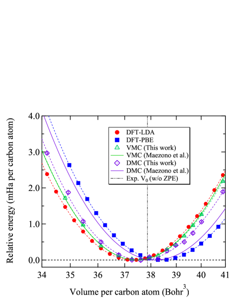
Figure 2: Equation of states and the curves fitted by the Vinet exponential function Vinet et al. (1987). VMC and DMC results (Maezono et al.) are taken from Ref. Maezono et al., 2007.

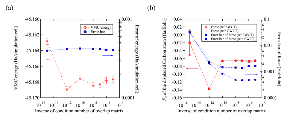
Figure 3: (a) VMC energies and their statistical error bars and (b) VMC forces and their statistical error bars vs. inverse of the condition number of the overlap matrix. The numerical data is shown in Table S-II foo . The forces were calculated with and without the space warp coordinate transformations (SWCT) Sorella and Capriotti (2010). The Hellmann-Feynman and Pulay contributions to the forces are shown in Fig. S-7 foo . The same VTZ atomic basis set and the pseudo potential Burkatzki et al. (2007) as in the phonon and EOS calculations were adopted, while 1 $\times$ 1 $\times$ 1 conventional cell (8 carbon atoms in a simulation cell) with $k$ = $\Gamma$ twist was employed. Only one carbon atom was displaced in $x$ direction by 0.15 bohr (Table S-III) foo .

Fig. 1 shows the phonon dispersion obtained by our VMC calculations using the conventional 2 $\times$ 2 $\times$ 2 diamond supercell . Observed experimental frequencies Warren et al. (1967); Liu et al. (2000); Kulda et al. (2002) are also plotted for comparison. A phonon dispersion obtained by the finite displacement method does not include anharmonic effects, which can decrease harmonic frequencies by up to $\sim$ 5-10% for the lightest elements Harris (1995). Therefore, for comparison with the experimental results, anharmonic corrections were added to the VMC phonon dispersion in this study. The phonon dispersion before the correction is shown in Fig. S-1 foo The anharmonic renormalizations were estimated in this study using path integral molecular dynamics simulationsMouhat et al. (2017); Morresi et al. at the DFT level with the PBE exchange-correlation function (Fig. S-5 foo ), giving $-$0.411 THz, $-$0.177 THz, and $-$0.280 THz for $\Gamma$, $X$, and $L$, respectively (see the SI for details). The value at $\Gamma$ is consistent with a reported estimate of $-$17.4 cm^-1 = $-$0.522 THz  Vanderbilt et al. (1984). Notice that other possible sources of error were also considered. The phonon dispersion in Fig. 1 also includes the one-body finite size corrections that were estimated by DFT calculations (see Fig. S-2 foo ) The two-body finite-size error is negligible because the average density and the volume do not change in phonon calculations. Table 1 shows a detailed comparison of the highest harmonic phonon frequencies at three $q$ points, i.e., $\Gamma$ = (0,0,0), $X$ = (2$\pi$,0,0), and $L$ = ($\pi$,$\pi$,$\pi$). Raman frequencies at $\Gamma$ obtained by a direct fit of VMC energies, VMC forces, and LRDMC energies of the structures displaced along the corresponding eigenmode are also plotted in Fig. 1. In Table 1 and hereafter, (P) denotes the interpolated frequencies obtained by Phonopy, (F) denotes the phonon frequency at $\Gamma$ obtained by force fitting, and (E) denotes the phonon frequency at $\Gamma$ obtained by energy fitting. The corresponding Raman frequencies are consistent within the error bars, indicating that the Slater determinant obtained by DFT is almost optimal also in the presence of the Jastrow factor, thus explaining why this consistency is satisfied quite accurately Moroni et al. (2014). In other words, if the wavefunction is at its minimum, the consistency is a consequence. If it is not at its minimum, the consistency may also be satisfied by chance or good behavior of the used basis set.

All VMC(P), VMC(F), and VMC(D) calculations give the harmonic phonon frequency at $\Gamma$ very close to the experimental value, considering the renormalization of the anharmonic effect, i.e., the discrepancy is just $\sim$ 0.3 THz. On the other hand, both DFT calculations with LDA-PZ and GGA-PBE exchange-correlation functionals underestimate the highest frequency at $\Gamma$ by $\sim$ 1.8 THz and $\sim$ 1.5 THz, respectively. Table 1 shows that our VMC phonon dispersion calculation also gives accurate harmonic frequencies at other $q$ points, i.e., at $X$ and $L$. Compared with the previous VMC study Maezono et al. (2007), our VMC frequency at $\Gamma$ point is closer to the experimental value, as reported in Table 1. The improvement at the VMC level certainly derives from the more flexible Jastrow factor employed in this study, while the one used in the previous VMC study was much simpler Drummond et al. (2004); Maezono et al. (2007).

It is intriguing that our LRDMC calculation gives a 1.2(2) THz higher Raman frequency than the experimental one, as shown in Table 1. The previous DMC study also overestimated the Raman frequency by 0.9(1) THz Maezono et al. (2007). To discuss the origin of the discrepancy, we investigated the effect of the lattice-space error in our LRDMC calculations. An extrapolation ($a\to 0$) with four lattice spaces (i.e., 0.20, 0.30, 0.40, and 0.50 bohr) yields 41.89(44) THz, suggesting that the lattice-space error is not the origin of the discrepancy. We also suspected that the experimental lattice parameter employed in the phonon calculation could be significantly different from the theoretical one, but this is also not the origin, as shown later. Therefore, the discrepancy should arise from the fixed-node error and this should be alleviated by a nodal surface optimization Nakano et al. (2020b), which however is prohibitive in the 2 $\times$ 2 $\times$ 2 conventional supercells due to the large number of variational parameters of the distorted structures. A possible future work to study the nodal surface effect is the use of various exchange-correlation functionals suitable for solids such as HSE06 Krukau et al. (2006) and SCAN Sun et al. (2015)

Since the equilibrium lattice parameter also affects phonon frequencies, we investigated the equation of states (EOSs) of diamond. Figure 2 shows plots of internal energies vs. volumes fitted by the Vinet EOS foo Previous VMC and DMC results Maezono et al. (2007), and the experimentally observed equilibrium lattice parameter are also plotted in Fig. 2 and summarized in Table 2. In Fig. 2, the zero point energy (ZPE) contributionMaezono et al. (2007); Hao et al. (2012) is subtracted, to make the comparison possible with internal energies computed at $T=0$ and on static lattice. Table 2 shows that our VMC calculation reproduces the previous VMC study, while our LRDMC calculation gives a slightly smaller lattice parameter (6.702(1) bohr) than the previous DMC study (6.734(4) bohr). This discrepancy likely derives from the different nodal surfaces used in the two studies, namely the one originating from the DFT-PBE orbitals in Ref. Maezono et al., 2007 and the one coming from the LDA orbitals in our work. Notice that both one-body and two-body finite size errors are negligible for the EOS calculations as shown in Fig. S-6 foo Table 2 indicates that the equilibrium lattice parameter of diamond is $\sim$ 0.03 bohr ($\sim$ 0.02 bohr) smaller than the experimental one at the VMC (LRDMC) level. Our DFT calculations (Fig. S-4 foo ) suggest that the Raman frequency is implicitly proportional to the lattice parameter, with a gradient of $-$0.18 THz/0.01 bohr. Therefore, if the equilibrium lattice parameter (with ZPE) were employed instead of the experimental one, VMC (LRDMC) calculations would give $\sim$ 0.5 THz ($\sim$ 0.4 THz) higher Raman frequencies, while still staying close to the experimental values.

Reducing the statistical errors of atomic forces is key to a successful phonon calculation. We found that alleviating the linear dependency of a localized atomic basis set drastically decreases the statistical error. In general, a basis set optimized for molecular systems is not suitable for solid state calculations, (i.e., strongly linear dependent) due to the presence of orbitals having small exponents (c.f., typically $<$ 0.1) Peintinger et al. (2013). The quality of the basis set is systematically improved by a general and efficient scheme implemented in TurboRVB Azadi et al. (2010). Indeed, the linear dependency of a localized atomic basis set ($\psi_{\mu}(\vec{r})$) is characterized by the condition number, $\kappa({\bf S})$, where $S_{\mu,\nu}=\braket{\psi_{\mu}}{\psi_{\nu}}$ is the overlap matrix . In TurboRVB, a redundant basis set is converted into a well-conditioned one, by disregarding small eigenvalues and the corresponding eigenvectors of the overlap matrix ${\bf S}$  Azadi et al. (2010); Nakano et al. (2020b). We note that a well-conditioned basis set can also be constructed by simply removing orbitals having small exponents, while the method employed in this work is more general and systematic. Figure 3 shows the plots of VMC energies, VMC forces, and their statistical errors vs. the inverse of the condition number ($\kappa({\bf S})^{-1}$). Figure 3 (a) indicates that the statistical error of the energy is independent of the condition number, at variance with the statistical error of the force, which instead strongly depends on it (Fig. 3 (b)). The error bar in the forces amounts to $\sim 3.4\times 10^{-2}$ (Ha/bohr) when the atomic basis set is strongly linear dependent (i.e., $\kappa({\bf S})^{-1}=10^{-15}$), a condition that also introduces some bias in the forces because, as we have verified, they are no longer consistent with the finite difference energy derivatives for $\kappa({\bf S})^{-1}<10^{-12}$ (see Fig. 3b) On the other hand, the statistical error becomes much smaller $\sim 1.7\times 10^{-3}$ (Ha/bohr) by removing the linear dependency (i.e., $\kappa({\bf S})^{-1}=10^{-7}$). The space warp coordinate transformation (SWCT) Sorella and Capriotti (2010) is able to further reduce the statistical error. Indeed, Fig. 3 (b) shows that the error bar of the force becomes $\sim 4.1\times 10^{-4}$ (Ha/bohr) by using the SWCT algorithm combined with a well-conditioned basis set, corresponding to $\sim 10^{4}$ times more efficient computation than a bare force treatment.

We analyze now in detail the reason of this behavior. TurboRVB evaluates atomic forces in a differential form (i.e, by the algorithmic differentiation) Attaccalite and Sorella (2008); Sorella and Capriotti (2010):

$${F_{\alpha}}={\braket{\frac{{dE}}{{d{R_{\alpha}}}}}}_{\left|{\Psi}^{\bf{R}}\right|^{2}}\simeq{\braket{\frac{E\left({\bf{R}}+\Delta{\bf{R}_{\alpha}}\right)-E\left({\bf{R}}\right)}{{\Delta{R_{\alpha}}}}}}_{\left|{\Psi}^{\bf{R}}\right|^{2}},$$

where ${\bf{R}}=(R_{1},\ldots,R_{\alpha},\ldots)$ and $\Delta{\bf{R}_{\alpha}}=(0,\ldots,\Delta R_{\alpha},\ldots)$. This equation suggests that the statistical error on forces depends on how much the wavefunction changes after an atom is displaced. In other words, to minimize the stochastic error, the overlap $\braket{\Psi^{{\bf{R}}+\Delta{\bf{R_{\alpha}}}}}{\Psi^{\bf{R}}}$ should be close to unity. To investigate the effect of the linear dependency on the overlap, we calculated $\braket{\Psi^{{\bf{R}}+\Delta{\bf{R}}_{\alpha}}}{\Psi^{\bf{R}}}$ with linear-dependent and linear-independent basis sets, using correlated sampling techniques Nakano et al. (2020b), where only one carbon atom in the 1 $\times$ 1 $\times$ 1 conventional simulation cell was displaced in the $x$ direction by $\Delta R_{\alpha}=0.005$ bohr. We obtained 0.9999 and 0.9726 for $\kappa({\bf S})^{-1}=10^{-7}$ and $\kappa({\bf S})^{-1}=10^{-15}$, respectively. This clearly indicates that the linear dependency of the basis set deteriorates the overlap $\braket{\Psi^{{\bf{R}}+\Delta{\bf{R}}_{\alpha}}}{\Psi^{\bf{R}}}$, thus increasing the statistical error of forces.

The deterioration is explained as follows: Here, a simple Slater wavefunction without Jastrow factor is considered for the sake of clarity. In this case, the overlap $\braket{\Psi^{{{\bf{R}}}}}{{\Psi^{{{\bf{R}}}}}}$ reads $\braket{\Psi^{{{\bf{R}}}}}{{\Psi^{{{\bf{R}}}}}}={\rm det}\langle\phi_{i}^{\bf{R}}|\phi_{j}^{\bf{R}}\rangle,$ where $\phi_{i}^{\bf{R}}$ is the $i$-th molecular orbital depending on nuclear positions R, defining the above $N\times N$ determinant matrix. The molecular orbital is expanded over localized atomic orbitals, i.e., $\phi_{i}^{\bf{R}}=\sum_{a,l}{c_{i,\{a,l\}}}\psi_{\{a,l\}}^{R_{a}}$, where $\psi_{\{a,l\}}^{R_{a}}$ are (periodized) atomic orbitals explicitly dependent on a nuclear position $R_{a}$ $\{a=1,\ldots,\alpha,\ldots\}$, while $c_{i,\{a,l\}}$ are nuclear position independent. We can readily derive $\braket{\Psi^{{{\bf{R}}}}}{{\Psi^{{{\bf{R}}}}}}=1$ when the molecular orbitals are orthonormalized (i.e., $\braket{\phi_{i}^{{{\bf{R}}}}}{\phi_{j}^{{{\bf{R}}}}}=\delta_{i,j}$). What about $\braket{\Psi^{{{\bf{R}}+\Delta{\bf{R_{\alpha}}}}}}{{\Psi^{{{\bf{R}}}}}}$? We would like to show how the perturbation $\frac{d}{d_{R_{\alpha}}}\phi_{i}^{\bf{R}}\equiv\sum_{a=\alpha,l}{c_{i,\{a,l\}}}\frac{d}{d_{R_{\alpha}}}\psi_{\{a,l\}}^{R_{a}}$ affects the overlap. In DFT calculations, it turns out that $\left|c_{i,\{a,l\}}\right|\gg 1$ when the basis is redundant (e.g., $\kappa({\bf S})^{-1}=10^{-15}$), while $\left|c_{i,\{a,l\}}\right|\ll 1$ when the basis set is well-conditioned (e.g., $\kappa({\bf S})^{-1}=10^{-7}$). When $\left|c_{i,\{a,l\}}\right|\ll 1$, the perturbation effect is rather small, and the orthonormalization condition almost holds, while $\left|c_{i,\{a,l\}}\right|\gg 1$ makes the perturbation effect significant, and by consequence the orthonormalization condition is certainly deteriorated. This is why the linear dependency of an atomic basis set deteriorates the overlap and, thus, induces a large error bar in forces. Thus, a complete all-electron and pseudopotential basis set database suitable for QMC solid state calculations will be quite useful for the application of QMC-forces to the calculations of phonons in realistic materials.

In summary, we report a VMC determination of the momentum-resolved phonon dispersion of diamond. Our approach combines the ab initio quantum Monte Carlo framework with the so-called frozen phonon technique. It gives results in very good agreement with experiments and provides renormalized harmonic optical frequencies consistent with the experimental findings. We estimated the purely harmonic contribution to the phonon spectrum, by evaluating $q$-dependent anharmonic corrections by means of a path integral molecular dynamics driven by PBE forcesMorresi et al. . After including these corrections, the VMC phonon spectrum agrees very well with the experimental phonon dispersion. We found that alleviating the atomic basis-set redundancy of the trial wavefunction is key to reduce the statistical error of atomic forces and, thus, to make the VMC phonons calculations feasible over the full Brillouin zone. This achievement paves the way to new relevant applications, for instance, in correlated materials and Van der Waals crystals (i.e., molecular crystals Subedi and Boeri (2011); Casula et al. (2012)), where sometimes phonons are poorly reproduced within the DFT framework.

Appendix A Details of QMC calculations

All Variational Monte Carlo (VMC) and lattice regularized diffusion Monte Carlo (LRDMC) Casula et al. (2005); Nakano et al. (2020a) calculations in this study were performed by a SISSA quantum Monte Carlo package, called TurboRVB  Nakano et al. (2020b). The package employs a many-body WF ansatz $\Psi$ which can be written as the product of two terms, i.e., $\Psi=\Phi_{\text{AS}}\times\exp J\,,$ where the term $\exp J$ and $\Phi_{\text{AS}}$ are conventionally called Jastrow and antisymmetric parts, respectively. The antisymmetric part is denoted as the Antisymmetrized Geminal Power (AGP) that reads: ${\Psi_{{\text{AGP}}}}\left({{{\mathbf{r}}_{1}},\ldots,{{\mathbf{r}}_{N}}}\right)={\hat{A}}\left[{\Phi\left({{\mathbf{r}}_{1}^{\uparrow},{\mathbf{r}}_{1}^{\downarrow}}\right)\Phi\left({{\mathbf{r}}_{2}^{\uparrow},{\mathbf{r}}_{2}^{\downarrow}}\right)\cdots\Phi\left({{\mathbf{r}}_{N/2}^{\uparrow},{\mathbf{r}}_{N/2}^{\downarrow}}\right)}\right],$ where ${\hat{A}}$ is the antisymmetrization operator, and $\Phi\left({{\mathbf{r}}^{\uparrow},{\mathbf{r}}^{\downarrow}}\right)$ is called the paring function Casula and Sorella (2003). The spatial part of the geminal function is expanded over the Gaussian-type atomic orbitals: ${\Phi_{{\text{AGP}}}}\left({{{\mathbf{r}}_{i}},{{\mathbf{r}}_{j}}}\right)=\sum\limits_{l,m,a,b}{{f_{\left\{{a,l}\right\},\left\{{b,m}\right\}}}{\psi_{a,l}}\left({{{\mathbf{r}}_{i}}}\right){\psi_{b,m}}\left({{{\mathbf{r}}_{j}}}\right)}$ where ${\psi_{a,l}}$ and ${\psi_{b,m}}$ are primitive Gaussian atomic orbitals, their indices $l$ and $m$ indicate different orbitals centered on atoms $a$ and $b$, and $i$ and $j$ are coordinates of spin up and down electrons, respectively, and ${{f_{\left\{{a,l}\right\},\left\{{b,m}\right\}}}}$ are the variational parameters. In this study, a triple-zeta basis set (11$s$11$p$2$d$1$f$) accompanying an energy-consistent pseudo potential Burkatzki et al. (2007) was employed for the atomic orbitals of the antisymmetric part (Table S-I). The pairing function can be also written as ${\Phi_{{\text{AGPn}}}}\left({{{\mathbf{r}}_{i}},{{\mathbf{r}}_{j}}}\right)=\sum_{k=1}^{M}\lambda_{k}\phi_{k}(\mathbf{r}_{i})\phi_{k}(\mathbf{r}_{j})$ with $\lambda_{k}>0$, where $\phi_{k}(\mathbf{r})$ is a molecular orbital, i.e., $\phi_{k}(\mathbf{r})=\sum_{i=1}^{L}{c_{i,k}{\psi_{i}}(\mathbf{r})}$. When the paring function is expanded over $M$ molecular orbitals where $M$ is equal to the half of the total number of electrons ($N/2$), the AGP coincides with the Slater-Determinant ansatz Becca and Sorella (2017); Marchi et al. (2009). In this study, we restricted ourselves to a Jastrow-Slater determinant (JSD) by setting $M=\frac{1}{2}\cdot N$, wherein the coefficients of atomic orbitals, i.e., ${c_{i,k}}$, were obtained by a Density Functional theory (DFT) calculation, and were fixed during a VMC optimization.

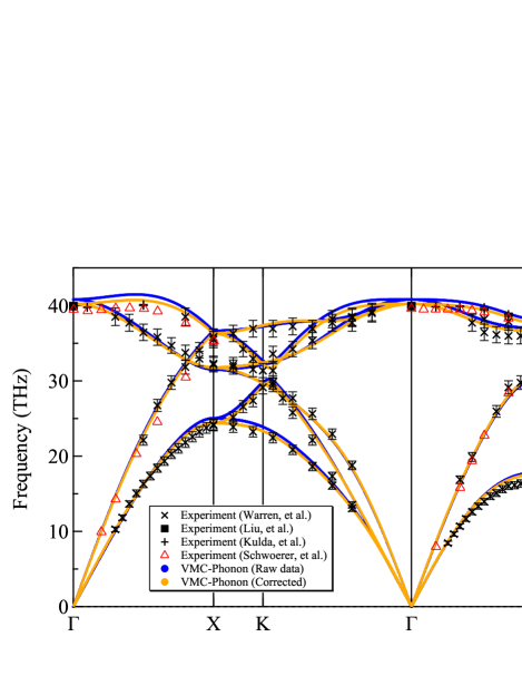
Figure S-1: The phonon dispersions of diamond calculated using 2 $\times$ 2 $\times$ 2 conventional supercell at the VMC level. “Raw data” denotes the phonon dispersion obtained by the finite-displacement method, while “Corrected” is the phonon dispersion where the anharmonic and one-body finite-size corrections are included. The error bars are not shown here for the sake of clarity. Observed experimental results are also plotted for comparison. Experimental data are taken from Refs. Warren et al., 1965; *1967WAR; Liu et al., 2000; Kulda et al., 2002; Schwoerer-Böhning et al., 1998. The data in Ref. Schwoerer-Böhning et al., 1998 were digitalized using WebPlotDigitizer Rohatgi (2020).

Table S-I: The valence triple-zeta (VTZ) uncontracted basis set (11$s$11$p$2$d$1$f$) used for the determinant part in the present work.

Orbital type	Exponent	Orbital type	Exponent
$s$	13.073594	$p$	1.871016
$s$	6.541187	$p$	0.935757
$s$	3.272791	$p$	0.468003
$s$	1.637494	$p$	0.376742
$s$	0.921552	$p$	0.234064
$s$	0.819297	$p$	0.126772
$s$	0.409924	$p$	0.117063
$s$	0.205100	$p$	0.058547
$s$	0.132800	$p$	0.029281
$s$	0.102619	$d$	1.141611
$s$	0.051344	$d$	0.329486
$p$	7.480076	$f$	0.773485
$p$	3.741035

The Jastrow term is composed of one-body, two-body and three/four-body factors ($J={J_{1}}{J_{2}}{J_{3/4}}$). The one-body and two-body factors are essentially used to fulfill the electron-ion and electron-electron cusp conditions, respectively, and the three/four-body factor is employed to consider further electron-electron correlations (e.g., electron-nucleus-electron). Since we employed an energy-consistent pseudo potential developed by Burkatzki et al. Burkatzki et al. (2007), we used only the inhomogeneous part of ${J_{1}^{inh}}$, $J_{2}$ and $J_{3/4}$ in this study (i.e., no electron-ion cusp corrections are needed). The inhomogeneous one-body Jastrow factor ${J_{1}^{inh}}$ reads ${J_{1}^{inh}}\left({{{\mathbf{r}}_{1}},\ldots,{{\mathbf{r}}_{N}}}\right)=\sum_{i=1}^{N}\sum_{a=1}^{N_{\text{atom}}}\left({\sum\limits_{l}{M_{a,l}\chi_{a,l}\left({{{\mathbf{r}}_{i}}}\right)}}\right),$ where ${{{\mathbf{r}}_{i}}}$ are the electron positions, ${{{\mathbf{R}}_{a}}}$ are the atomic positions with corresponding atomic number $Z_{a}$, $l$ runs over atomic orbitals $\chi_{a,l}$ (e.g., GTO) centered on the atom $a$, ${N_{\text{atom}}}$ is the total number of atoms in a system, and $\{M_{a,l}\}$ are variational parameters. The two-body Jastrow factor is defined as: ${J_{2}}\left({{{\mathbf{r}}_{1}},\ldots{{\mathbf{r}}_{N}}}\right)=\exp\left({\sum\limits_{i<j}{v\left({\left|{{{\mathbf{r}}_{i}}-{{\mathbf{r}}_{j}}}\right|}\right)}}\right),$ where $v\left(r\right)$ is $v\left(r\right)=\frac{1}{2}r\cdot{\left({1-F\cdot r}\right)^{-1}}$ and $F$ is a variational parameter. The three-body Jastrow factor is: ${J_{3/4}}\left({{{\mathbf{r}}_{1}},\ldots{{\mathbf{r}}_{N}}}\right)=\exp\left({\sum\limits_{i<j}{{\Phi_{{\text{Jas}}}}\left({{{\mathbf{r}}_{i}},{{\mathbf{r}}_{j}}}\right)}}\right),$ and ${\Phi_{{\text{Jas}}}}\left({{{\mathbf{r}}_{i}},{{\mathbf{r}}_{j}}}\right)=\sum\limits_{l,m,a,b}{g_{a,l,m,b}\chi_{a,l}^{{\text{Jas}}}\left({{{\mathbf{r}}_{i}}}\right)\chi_{b,m}^{{\text{Jas}}}\left({{{\mathbf{r}}_{j}}}\right)},$ where the indices $l$ and $m$ again indicate different orbitals centered on corresponding atoms $a$ and $b$. In this study, the coefficients of the three/four-body Jastrow factor were set to zero for $a\neq b$ because it significantly decreases the number of variational parameters while rarely affects variational energies . A basis set (3$s$2$p$) was employed for the atomic orbitals of the Jastrow part. The variational parameters in the Jastrow factor were optimized by the so-called stochastic reconfiguration Sorella et al. (2007) and/or the modified linear method Umrigar et al. (2007); Nakano et al. (2020b) implemented in TurboRVB. Using the optimized wavefunction, energies and forces are calculated at the VMC and the LRDMC levels. All LRDMC calculations were performed by the original single-grid scheme Casula et al. (2005) with the discretization grid size $a=0.20$ Bohr. For the Raman frequency calculation, several lattice spaces, i.e., $a$ = 0.20, 0.30, 0.35, 0.40, and 0.50 Bohr were also used to extrapolate the energies (i.e., $a\to 0$) with a quadratic function (i.e., $E(a)=E_{0}+k_{1}\cdot a^{2}+k_{2}\cdot a^{4}$).

Figure S-1 shows the phonon dispersions and Raman frequencies of diamond calculated using 2 $\times$ 2 $\times$ 2 conventional supercell at the VMC level. “Raw data” denotes the phonon dispersion obtained by the finite-displacement method, while “Corrected” is the phonon dispersion where the one-body finite-size (see sec. B) and anharmonic (see sec. C) corrections are included.

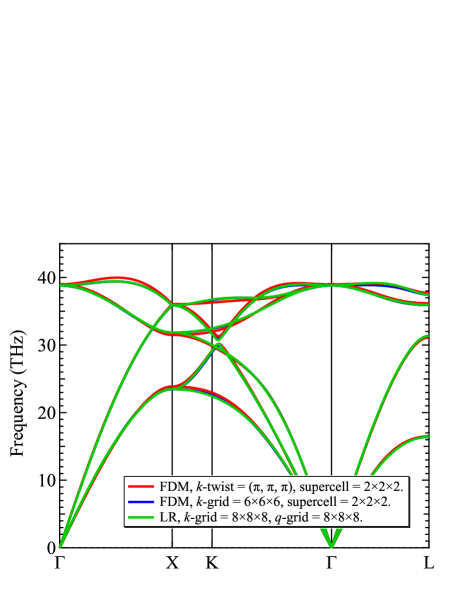
Figure S-2: Phonon dispersions of diamond obtained by different methods with different computational conditions at the DFT level, wherein the experimental lattice parameter was used. (a) A phonon dispersion calculated by the finite-displacement method (FDM), or the so-called frozen-phonon method, implemented in Phonopy Togo and Tanaka (2015) with 2 $\times$ 2 $\times$ 2 conventional supercell at $L$ point. The displacement of 0.03 Bohr was employed for calculating derivatives of atomic forces with respect to a nucleus position. (b) The same as (b) except for $k$-grid. The shifted 6 $\times$ 6 $\times$ 6 Monkhorst-Pack grid Monkhorst and Pack (1976) was employed. (c) A phonon dispersion calculated by the linear response method implemented Quantum Espresso package Giannozzi et al. (2009) with 1 $\times$ 1 $\times$ 1 primitive unit cell. The shifted (unshifted) 8 $\times$ 8 $\times$ 8 Monkhorst-Pack grid Monkhorst and Pack (1976) was employed for $k$-integration ($q$-interpolation). The DFT calculations were performed with GGA-PBE functionals with Ultrasoft (US) pseudo potential taken from PS-Library Dal Corso (2014).

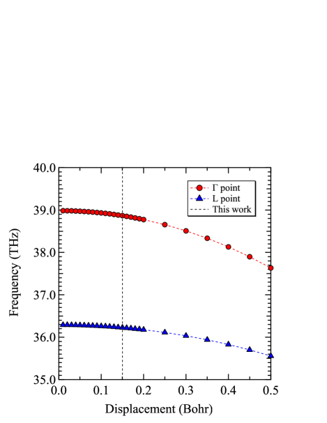
Figure S-3: Phonon frequencies calculated by DFT at $q$ = $\Gamma$ and $L$ points v.s. employed displacements in the finite displacement method, where the GGA-PBE functional was employed. The phonon dispersions were calculated using 2 $\times$ 2 $\times$ 2 conventional supercell with $k$ twist = $L$ ($\pi$,$\pi$,$\pi$).

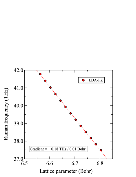
Figure S-4: Plots of Raman Frequencies vs. lattice parameters of diamond. They were calculated using the linear response theory implemented in Quantum Espresso at a single $q$ point, i.e., $q$ = (0,0,0) with the LDA-PZ exchange-correlation functional. The primitive lattice was employed with $k$-grid = 8 $\times$ 8 $\times$ 8.

Appendix B Validation of computational conditions using DFT.

There are two major implementations to compute a harmonic phonon dispersion, i.e., the finite displacement method (FDM) and the linear response method. The former is also called frozen phonon method. Their results should be consistent as far as employed hyperparameters are correct. Figure S-2 shows phonon dispersions of diamond obtained by the two different methods at the DFT level, wherein the experimental lattice parameter was used. (a) A phonon dispersion calculated by the frozen-phonon method implemented in Phonopy Togo and Tanaka (2015) with 2 $\times$ 2 $\times$ 2 conventional supercell at $L$ point. The displacement of 0.03 Bohr was employed for calculating derivatives of atomic forces with respect to a nucleus position. (b) The same as (a) except for $k$-grid. The shifted 6 $\times$ 6 $\times$ 6 Monkhorst-Pack grid Monkhorst and Pack (1976) was employed. (c) A phonon dispersion calculated by the linear response method implemented Quantum Espresso package Giannozzi et al. (2009) with 1 $\times$ 1 $\times$ 1 primitive unit cell. The 8 $\times$ 8 $\times$ 8 Monkhorst-Pack grids Monkhorst and Pack (1976) were employed for $k$ and $q$ integrations. The DFT calculations were performed with GGA-PBE functionals with Ultrasoft (US) pseudo potential taken from PS-Library Dal Corso (2014). Comparison of (a)-red with (c)-green proves that the one-body finite size error is very small in a phonon calculation thanks to the error cancellation when $L$ twist for 2 $\times$ 2 $\times$ 2 conventional supercell is employed. In detail, the one-body finite size errors are 0.16 THz, 0.18 THz, and 0.23 THz for $q$ = $\Gamma$, $X$, and $L$, respectively. Comparison of (b)-blue with (c)-green, which are almost overlapped, suggests that the finite difference method does not bias the result. As mentioned in the main text, 0.15 Bohr was employed for the displacement of a carbon atom in the VMC frozen-phonon calculation to decrease the statistical error. Figure. S-3 shows the amplitude of 0.15 Bohr employed underestimates frequencies by $\sim$ 0.12 THz. A single-phonon phonon calculation at $\Gamma$ alleviates this underestimation as mentioned in the main text. Fig. S-4 shows a plot of Raman Frequencies vs. lattice parameters of diamond. They were calculated using the linear response theory implemented in Quantum Espresso at a single $q$ point, i.e., $q$ = (0,0,0) with the LDA-PZ exchange-correlation functional. The primitive lattice was employed with 8 $\times$ 8 $\times$ 8.

Appendix C Anharmonic renormalizations from path integral molecular dynamics

The anharmonic renormalizations of phonon frequencies reported in Table 1 with the superscript ’$f$’ were computed through the displacement-displacement zero-time Kubo-correlator built upon path integral molecular dynamics (PIMD) trajectories. The evaluation of the displacement-displacement correlator over classical molecular dynamics trajectories is a standard method to predict force constant matrices and phonon spectra, but it misses nuclear quantum effects. The details of the extension of such a method to extract phonon dispersions from path integral molecular dynamics can be found in Ref. Morresi et al., .

In Fig S-5, we report the whole spectrum that we have obtained using this new approach compared to the linear response DFT curve.

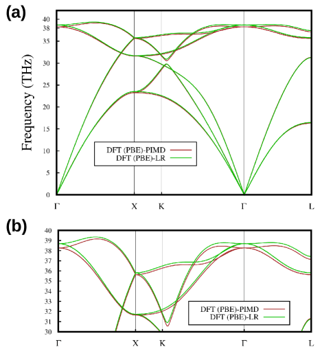
Figure S-5: (a) Phonon spectrum at 300 K obtained from PIMD simulation versus linear response (LR) DFT spectrum; (b) Zoom over the optical modes.

In particular, the ion equations of motion were integrated using the PIOUD algorithm Mouhat et al. (2017), while at each time step the electronic potential energy surface was evaluated at DFT level using the Quantum Espresso package Giannozzi et al. (2009) and GGA-PBE Perdew et al. (1996) exchange-correlation functionals. The simulation was carried out at 300 Kelvin for 34 picoseconds employing 12 beads. We used the same 64-atoms supercell as for the QMC calculations, with a 2 $\times$ 2 $\times$ 2 $k$-grid for electronic integration and a cutoff for wavefunctions equal to 60 Ry.

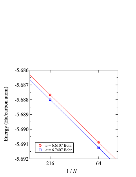
Figure S-6: Finite-size extrapolation for different lattice parameters. The differences of energies are constant regardless of the simulation cell size, indicating that the finite-size error is negligible for an EOS calculation thanks to the error cancellation. Since diamond is an insulator, raw QMC energies obtained at $L$ point can be smoothly extrapolated by a linear function. See. Ref. Hennig et al., 2010

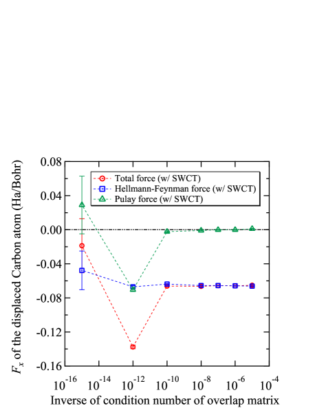
Figure S-7: VMC forces, its Hellmann-Feynman, and its Pulay contributions v.s. inverse of the condition number of the overlap matrix. The forces were calculated with the space warp coordinate transformations (SWCT) Sorella and Capriotti (2010). The same VTZ atomic basis set and the pseudo potential Burkatzki et al. (2007) as in the phonon and EOS calculations were adopted, while 1 $\times$ 1 $\times$ 1 conventional cell (8 carbon atoms in a simulation cell) with $k$ = $\Gamma$ twist was employed. Only one carbon atom was displaced in $x$ direction by 0.15 Bohr.

Table S-II: Error bars of forces corresponding to Fig. 3(b) in the main text. $\kappa({\bf S})^{-1}$ denotes the inverse of the condition number of the overlap matrix ${\bf S}$. The used geometry is showin in Table S-III

$\kappa({\bf S})^{-1}$	with SWCT		without SWCT
	Force ($F_{x}$ of C1) (Ha/bohr)	Error bar (Ha/bohr)	Force ($F_{x}$ of C1) (Ha/bohr)	Error bar (Ha/bohr)
$10^{-5}$	-6.659 $\times$ $10^{-2}$	4.1 $\times$ $10^{-4}$	-6.71 $\times$ $10^{-2}$	1.7 $\times$ $10^{-3}$
$10^{-6}$	-6.622 $\times$ $10^{-2}$	4.1 $\times$ $10^{-4}$	-6.67 $\times$ $10^{-2}$	1.4 $\times$ $10^{-3}$
$10^{-7}$	-6.523 $\times$ $10^{-2}$	4.4 $\times$ $10^{-4}$	-6.68 $\times$ $10^{-2}$	1.3 $\times$ $10^{-3}$
$10^{-8}$	-6.635 $\times$ $10^{-2}$	4.6 $\times$ $10^{-4}$	-6.77 $\times$ $10^{-2}$	1.5 $\times$ $10^{-3}$
$10^{-10}$	-6.734 $\times$ $10^{-2}$	8.0 $\times$ $10^{-4}$	-6.59 $\times$ $10^{-2}$	1.6 $\times$ $10^{-3}$
$10^{-12}$	-13.87 $\times$ $10^{-2}$	1.8 $\times$ $10^{-3}$	-13.86 $\times$ $10^{-2}$	2.4 $\times$ $10^{-3}$
$10^{-15}$	-4.7 $\times$ $10^{-2}$	3.3 $\times$ $10^{-2}$	-4.9 $\times$ $10^{-2}$	3.4 $\times$ $10^{-2}$

Appendix D Finite-size errors in QMC calculations

The effect of the finite-size errors on an EOS calculation has been investigated. Figure S-6 shows that finite-size extrapolations for two different lattice parameters ($a$ = 6.6107 and 6.7407 Bohr). The differences of the energies are constant regardless of the simulation cell size, indicating that the finite-size error is negligible for an EOS calculation thanks to the error cancellation. Since diamond is an insulator, raw QMC energies obtained at $L$ point can be smoothly extrapolated by a linear function. See. Ref. Hennig et al., 2010.

Appendix E Vinet exponential function

In this study, the obtained energies were fitted by the Vinet exponential function Vinet et al. (1987) that reads:

$$E(V) = E_{0}+\frac{2B_{0}V_{0}}{\left(B_{0}^{\prime}-1\right)^{2}}\left\{2-\left[5+3\left(\frac{V}{V_{0}}\right)^{\frac{1}{3}}(B_{0}^{\prime}-1)-3B_{0}^{\prime}\right]\right.$$

$$\times \left.\exp\left[-\frac{3}{2}\left(B_{0}^{\prime}-1\right)\left[\left(\frac{V}{V_{0}}\right)^{\frac{1}{3}}-1\right]\right]\right\},$$

where $E(V)$ is the total energy per atom, $V$ is volume per atom, and $E_{0}$, $V_{0}$, $B_{0}$, and $B_{0}^{\prime}$ are parameters. The non-linear fittings were performed using SciPy module Virtanen et al. (2020) implemented in Python.

Appendix F Atomic forces

TurboRVB evaluates atomic forces in a differential expression Sorella and Capriotti (2010):

$${{\mathbf{F}}_{a}}=-\left\langle{\frac{d}{{d{{\mathbf{R}}_{a}}}}{e_{L}}}\right\rangle+2\left({\left\langle{{e_{L}}}\right\rangle\left\langle{\frac{d}{{d{{\mathbf{R}}_{a}}}}\ln\left({{{\mathcal{J}}^{\frac{1}{2}}}\Psi}\right)}\right\rangle-\left\langle{{e_{L}}\frac{d}{{d{{\mathbf{R}}_{a}}}}\ln\left({{{\mathcal{J}}^{\frac{1}{2}}}\Psi}\right)}\right\rangle}\right)$$

where ${\mathcal{J}}$ is the Jacobian of the space warp coordinate transformation (SWCT) Sorella and Capriotti (2010), ${e_{L}}$ is the local energy, and the brackets indicates a Monte Carlo average over the trial WF. The first term is called “Hellmann-Feynman” force (HF) and the second and third terms are called “Pulay” force (PF). All the terms above can be written by the partial derivatives of the local energy and those of the logarithm of the WF Sorella and Capriotti (2010). These differential expressions are efficiently computed in TurboRVB, by using the adjoint algorithmic differentiation technique Sorella and Capriotti (2010). TurboRVB also employs the so-called reweighting technique developed by Attaccalite and Sorella Attaccalite and Sorella (2008) to avoid divergence of the derivatives in the vicinity of the nodal surfaces. Fig. S-7 shows VMC forces, its Hellmann-Feynman, and its Pulay contributions v.s. inverse of the condition number of the overlap matrix, corresponding to Fig. 3 in the main text. Fig. S-7 clarifies that the erratic behavior of the forces at $\kappa({\bf S})^{-1}=10^{-12}$ comes from its Pulay contribution, indicating that the linear-dependency of a basis-set also deteriorates absolute values of forces.

Table S-III: The geometry of the displaced diamond used to obtain forces in Table S-II. The lattice parameter is 6.741 Bohr. $x$, $y$, and $z$ are represented by fractional coordinates.

Element	Label	$x$	$y$	$z$
C	C1	0.02225	0.00000	0.00000
C	C2	0.00000	0.50000	0.50000
C	C3	0.50000	0.00000	0.50000
C	C4	0.50000	0.50000	0.00000
C	C5	0.25000	0.25000	0.75000
C	C6	0.75000	0.75000	0.75000
C	C7	0.25000	0.75000	0.25000
C	C8	0.75000	0.25000	0.25000