From One to All: Learning to Match Heterogeneous
and Partially Overlapped Graphs

Abstract

Recent years have witnessed a flurry of research activity in graph matching, which aims at finding the correspondence of nodes across two graphs and lies at the heart of many artificial intelligence applications. However, matching heterogeneous graphs with partial overlap remains a challenging problem in real-world applications. This paper proposes the first practical learning-to-match method to meet this challenge. The proposed unsupervised method adopts a novel partial OT paradigm to learn a transport plan and node embeddings simultaneously. In a from-one-to-all manner, the entire learning procedure is decomposed into a series of easy-to-solve sub-procedures, each of which only handles the alignment of a single type of nodes. A mechanism for searching the transport mass is also proposed. Experimental results demonstrate that the proposed method outperforms state-of-the-art graph matching methods.

1 Introduction

Graph matching (network alignment), aiming to determine the correspondence of nodes across two related graphs, lies at the heart of a wide range of artificial intelligence applications, including network retrieval (Berretti, Del Bimbo, and Vicario 2001; Özer, Wolf, and Akansu 2002), machine translation (Bahdanau, Cho, and Bengio 2014; Chen et al. 2020), and visual tracking (Xiong et al. 2012; Wang and Ling 2017), to name a few. Two main algorithmic components, the node conservation and the matching strategy, constitute the graph matching method, where the former measures the similarity between pairs of nodes from different networks, and the later maximizes total node conservation over aligned nodes and the amount of conserved edges (Gu et al. 2018).

Mainstream methods of graph matching have followed two directions that correspond to different matching strategies. (i) One is the seed-and-extend strategy, which recursively matches nodes adjacent to the currently aligned subgraphs (Narayanan and Shmatikov 2009; Pedarsani and Grossglauser 2011; Yartseva and Grossglauser 2013; Sun et al. 2015). In general, incorrectly matched pairs could cause more mismatching in future steps, i.e., a cascade of errors (Kazemi 2016). (ii) The other is the searching strategy, which explores the entire alignment space and returns the one with the highest score based on a specific objective. In this paradigm, a few recent researches have shifted focus to settings in which the best searching is rephrased in the framework of optimal transport (OT) and the resulting algorithms have achieved the state-of-the-art performance (Xu et al. 2019; Titouan et al. 2019; Barbe et al. 2020), compared with its traditional counterparts such as simulated annealing (Mamano and Hayes 2017), genetic algorithm (Vijayan, Saraph, and Milenković 2015), or gradient-based optimization (Konar and Sidiropoulos 2020).

Despite this recent activity, the advances in methodology have been confined almost exclusively to the matching of homogeneous (containing only one type of nodes) or fully overlapped graphs, and none of existing methods has demonstrated its effectiveness on real-world alignment tasks in which graphs are both heterogeneous and partially overlapped. Such real-world tasks may include knowledge graph alignment (Li et al. 2018), matching of biological networks (Sharan and Ideker 2006), and disambiguating entities (Zhang, Swami, and Chawla 2019). We illustrate this situation in Figure 1 and depict technical details of these two challenges in the following paragraphs.

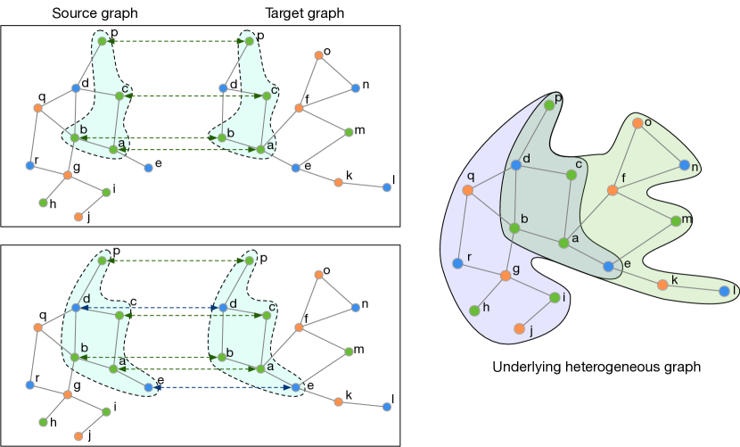
Figure 1: An illustration of the from-one-to-all matching strategy for both heterogeneous and partially overlapped graphs. The right sub-figure depicts an underlying heterogeneous graph. The color of each node indicates its type. The source graph and the target graph pictured in the left sub-figure are its two partially overlapped sub-graphs. For example, node r in the source graph does not exist in the target graph. First, type-green nodes are matched (top row of the left sub-figure). Then, type-blue nodes are matched (bottom row of the left sub-figure).

Heterogeneity.

Most existing methods consider graphs with only one type of nodes. Directly applying these methods to heterogeneous graphs leads to inferior performance and type mismatch. Gu et al. (2018) propose the first practical heterogeneous graph matching method based on manually designed features, called colored graphlet degree vectors (CGDV), and extend a large body of homogeneous algorithms (Sun et al. 2015; Vijayan, Saraph, and Milenković 2015; Mamano and Hayes 2017) into heterogeneous variants. The designed features, however, are expensive to obtain since the computational complexity for generating CGDV is practically $\mathcal{O}(V^{5})$, where $V$ is the number of nodes of the graph. Apparently, as $V$ increases, their performances will deteriorate rapidly. Besides, these methods cannot guarantee that there is no type mispairing. Thus, efficiently and effectively matching all types of nodes still remains a challenging problem.

Partial Overlapping.

Partial overlapping is another challenging problem, which is generally tackled by adding dummy nodes that act like wildcards to absorb unmatched nodes (Swoboda et al. 2017, 2019; Sarlin et al. 2020; Rolínek et al. 2020). However, this kind of methods still suffer from two intractable issues. First, they are usually supervised methods and require a large amount of ground truth node pairs. Second, they cannot constrain the number of matching pairs even if the prior information about the degree of overlap is already known, which may lead to some extreme cases. For example, zero matching would be identified to be an optimal result when dummy nodes are adopted.

To meet these challenges from real-world tasks, we propose a novel method to match heterogeneous graphs that are possibly partially overlapped. The proposed method adopts a novel partial OT scheme to learn a transport plan and node embeddings simultaneously. For the sake of computational efficiency, the entire learning procedure is decomposed into a series of easy-to-solve sub-procedures. Specifically, each sub-procedure only handles a homogeneous but possibly partially overlapped alignment problem, with a set of node pairs which are already matched in the previous sub-procedures as seeds. Essentially, this method proceeds by first matching one type of nodes and gradually matching other types until all types are matched, that is, from one to all types, so we name it FOTA. To boost robustness against noise and further reduce the cascade of errors, we also incorporate node embeddings which encode the global topology. Our contributions are summarized as follows.

1. FOTA is the first practical unsupervised method to match both heterogeneous and partially overlapped graphs, so far as we know, by using a hybrid strategy that mixes seed-and-extend and searching strategies. Compared to the principled method in (Gu et al. 2018), ours achieves no type mismatch at a very low cost. The overall complexities for updating the transport plan and the embeddings are $\mathcal{O}\big{(}N(T+k+d)V^{2}\big{)}$ and $\mathcal{O}(VBd)$ respectively.

2. A mechanism for searching the transport mass is also proposed, which endows our method a possibility to control the number of matching pairs according to some prior information. Thus the partial OT technique leveraged by our method only needs to transport an enough fraction of the mass with a minimum transportation cost.

Extensive experimental results demonstrate that the proposed method outperforms the state-of-the-art graph matching methods. The rest of the paper is organized as follows. In Sec. 2, a comprehensive review of background is given. The methodology of FOTA is presented in Sec. 3. Empirical results are demonstrated in both Sec. 4. We finally present related work in Sec. 5.

Notation.

We use bold lowercase symbols, bold uppercase letters, uppercase calligraphic fonts, and Greek letters to denote vectors, matrices, spaces (sets), and measures, respectively. $\mathbf{1}^{d}\in\mathbb{R}^{d}$ is an all-ones vector. The cardinality of set $\mathcal{A}$ is denoted by $|\mathcal{A}|$. $\mathbf{A}[i,:]$ and $\mathbf{A}[:,j]$ are the $i$-th row and the $j$-th column of matrix $\mathbf{A}$ respectively.

2 Preliminaries

2.1 Graph Matching

A graph is denoted as $\mathcal{G}=(\mathcal{V},\mathcal{E},\phi,\mathcal{T})$, where $\mathcal{V}$ is the set of nodes, $\mathcal{E}$ is the set of edges, $\mathcal{T}$ is the set of node types, and the type mapping function $\phi:\mathcal{V}\to\mathcal{T}$ assigns each node a type. When graph $\mathcal{G}$ contains multiple types of nodes, i.e., $|\mathcal{T}|\geq 2$, $\mathcal{G}$ is a heterogeneous graph; otherwise, it is a homogeneous graph. Assigning each node an index $i\in\{1,\dots,|\mathcal{V}|\}$, the edge set $\mathcal{E}$ can also be written as an adjacency matrix $\mathbf{W}\in\mathbb{R}^{|\mathcal{V}|\times|\mathcal{V}|}$ with entry $W_{ij}=1$ if and only if there is an edge connecting nodes $i$ and $j$.

Mathematically, graph matching finds a matching matrix $\mathbf{T}=[T_{ii^{\prime}}]$ between the source graph $\mathcal{G}^{\operatorname{s}}=(\mathcal{V}^{\operatorname{s}},\mathcal{E}^{\operatorname{s}},\phi^{\operatorname{s}},\mathcal{T})$ and the target graph $\mathcal{G}^{\operatorname{t}}=(\mathcal{V}^{\operatorname{t}},\mathcal{E}^{\operatorname{t}},\phi^{\operatorname{t}},\mathcal{T})$, where $T_{ii^{\prime}}=1$ if node $i\in\mathcal{V}^{\operatorname{s}}$ is matched to node $i^{\prime}\in\mathcal{V}^{\operatorname{t}}$, and $T_{ii^{\prime}}=0$ otherwise. Assuming $\mathcal{G}^{\operatorname{s}}$ has fewer nodes than $\mathcal{G}^{\operatorname{t}}$, the matching matrix is generally identified by minimizing the following loss function (Caetano et al. 2009)

$$\min_{\mathbf{T}\in\mathcal{P}^{f}}\bigg{[}\sum_{i,j=1}^{|\mathcal{V}^{\operatorname{s}}|}\sum_{i^{\prime},j^{\prime}=1}^{|\mathcal{V}^{\operatorname{t}}|}d_{ii^{\prime}jj^{\prime}}T_{ii^{\prime}}T_{jj^{\prime}}+\sum_{i=1}^{\mathcal{V}^{\operatorname{s}}|}\sum_{i^{\prime}=1}^{|\mathcal{V}^{\operatorname{t}}|}k_{ii^{\prime}}T_{ii^{\prime}}\bigg{]},$$ (1)

where $k_{ii^{\prime}}$ is the cost for the unary matching $i\rightarrow i^{\prime}$, $d_{ii^{\prime}jj^{\prime}}$ is the cost for the pairwise matching $(i,j)\rightarrow(i^{\prime},j^{\prime})$, and the feasible domain is

Such formulation matches every node in $\mathcal{G}^{\operatorname{s}}$ to exact one node in $\mathcal{G}^{\operatorname{t}}$ and hence is referred to as full matching (Kazemi, Yartseva, and Grossglauser 2015). For partial matching, generally $\mathcal{P}^{f}$ is replaced with the relaxed feasible domain

see e.g. (Kazemi, Yartseva, and Grossglauser 2015; Sarlin et al. 2020; Wang et al. 2020). Such formulation, however, may lead to matching no pairs in extreme cases. For example, when $d_{ii^{\prime}jj^{\prime}}>0$ and $k_{ii^{\prime}}>0$ for all $i,i^{\prime}j,j^{\prime}$, matching no nodes ($\mathbf{T}=\mathbf{0}$) is the optimal solution. Matching two heterogeneous graphs further requires $\phi^{\operatorname{s}}(i)=\phi^{\operatorname{t}}(i^{\prime})$ if node $i$ is matched to $i^{\prime}$.

2.2 Optimal Transport

Optimal Transport (OT) addresses the problem of transporting one measure toward another measure with the minimum cost (Villani 2008). The induced cost defines a distance between the two measures. A discrete measure $\alpha$ can be denoted by $\alpha=\sum_{i=1}^{m}p_{i}\delta_{\mathbf{x}_{i}}$ where $\delta_{\mathbf{x}}$ is the Dirac at position $\mathbf{x}$, i.e., a unit of mass infinitely concentrated at $\mathbf{x}$. With slight abuse of notation, we also use $\mathbf{p}=[p_{i}]$ to refer to $\alpha$.

Wasserstein distance.

The $p$-Wasserstein distance (Villani 2008; Cuturi 2013) between discrete measures $\mathbf{p}$ and $\mathbf{q}$ is defined as

$$\textstyle W_{p}^{p}(\mathbf{p},\mathbf{q})=\min_{\mathbf{T}\in\Pi(\mathbf{p},\mathbf{q})}\sum_{i=1}^{m}\sum_{i^{\prime}=1}^{n}K^{p}_{ii^{\prime}}T_{ii^{\prime}},$$

where $K_{ii^{\prime}}$ is the $\ell_{p}$ distance between $\mathbf{x}_{i}$ and $\mathbf{y}_{i^{\prime}}$ and the feasible domain of transport plan $\mathbf{T}=[T_{ii^{\prime}}]$ is given by the set $\Pi(\mathbf{p},\mathbf{q})=\{\mathbf{T}\in\mathbb{R}_{+}^{m\times n}|\mathbf{T}\mathbf{1}^{n}=\mathbf{p},\mathbf{T}^{\top}\mathbf{1}^{m}=\mathbf{q}\}$. The Wasserstein distance requires the supports of the two measures to be in the same space.

Gromov-Wasserstein distance.

Gromov-Wasserstein (GW) distance extends Wasserstein distance to compare measures supported in different spaces (Mémoli 2011). Let $\mathcal{X}$ and $\mathcal{Y}$ be two sample spaces. Endowing the spaces $\mathcal{X}$ and $\mathcal{Y}$ with metrics (distances) $d_{\mathcal{X}}$ and $d_{\mathcal{Y}}$, the GW distance is defined as

$$GW_{p}^{p}(\mathbf{p},\mathbf{q})=\min_{\mathbf{T}\in\Pi(\mathbf{p},\mathbf{q})}\sum_{i,j=1}^{m}\sum_{i^{\prime},j^{\prime}=1}^{n}D_{ii^{\prime}jj^{\prime}}^{p}T_{ii^{\prime}}T_{jj^{\prime}},$$

where $D_{ii^{\prime}jj^{\prime}}=|d_{\mathcal{X}}(\mathbf{x}_{i},\mathbf{x}_{j})-d_{\mathcal{Y}}(\mathbf{y}_{i^{\prime}},\mathbf{y}_{j^{\prime}})|$ with $\mathbf{x}_{1}$, $\mathbf{x}_{2}$, $\ldots$, $\mathbf{x}_{m}\in\mathcal{X}$ and $\mathbf{y}_{1}$, $\mathbf{y}_{2}$, $\ldots$, $\mathbf{y}_{n}\in\mathcal{Y}$.

OT-based graph matching.

By associating each graph with a discrete probability measure, OT can be applied to graph matching. Xu et al. (2019) propose a GW learning framework called GWL for graph matching. They correspond two graphs $\mathcal{G}^{\operatorname{s}}$ and $\mathcal{G}^{\operatorname{t}}$ to discrete probability measures $\mbox{\boldmath$\mu$\unboldmath}^{\operatorname{s}}=[\mu^{\operatorname{s}}_{i}]$ and $\mbox{\boldmath$\mu$\unboldmath}^{\operatorname{t}}=[\mu^{\operatorname{t}}_{i}]$ respectively, where

$$\mu^{z}_{i}=\frac{\sum_{j=1}^{|\mathcal{V}^{z}|}W_{ij}^{z}}{\sum_{i=1}^{|\mathcal{V}^{z}|}\sum_{j=1}^{|\mathcal{V}^{z}|}W_{ij}^{z}},$$

for $z={\operatorname{s}},{\operatorname{t}}$. By replacing the strict distances with dissimilarity functions, GWL relaxes the GW distance and the Wasserstein distance to the GW discrepancy and the Wasserstein discrepancy separately. Such relaxation allows GWL to incorporate node embeddings to parameterize the discrepancies and improve the robustness to the noise of edges. GWL uses the learned transport plan to indicate the node correspondence, i.e., $i^{\prime}\in\mathcal{V}^{\operatorname{t}}$ that receives the most mass from $i\in\mathcal{V}^{\operatorname{s}}$ is the estimated counterpart of $i$.

Both the Wasserstein distance and the GW distance require the two marginals $\mathbf{p}$ and $\mathbf{q}$ to have the same total mass, that is, $\|\mathbf{p}\|_{1}=\|\mathbf{q}\|_{1}$, thus all the mass has to be transported. By contrast, the partial OT problem focuses on transporting only a fraction $0\leq b\leq\min\{\|\mathbf{p}\|_{1},\|\mathbf{q}\|_{1}\}$ of the mass with the minimum transportation cost (Figalli 2010; Caffarelli and McCann 2010; Chapel, Gasso et al. 2020), that is, the set of admissible couplings is given by

$$\Pi^{b}(\mathbf{p},\mathbf{q})=\Big{\{}\mathbf{T}\in\mathbb{R}_{+}^{m\times n}\Big{|}\mathbf{T}\mathbf{1}\leq\mathbf{p},\mathbf{T}^{\top}\mathbf{1}\leq\mathbf{q},\mathbf{1}^{\top}\mathbf{T}\mathbf{1}=b\Big{\}}.$$

By adding a dummy node into the target graph, the mass of the nodes which have no counterparts in the target graph can be considered as being transported to the dummy node.

3 Methodology

We first introduce the underlying model in real-world scenarios for matching graphs that are heterogeneous and partially overlapped. Next, we derive a practical from-one-to-all model by decomposing the learning procedure into a series of interrelated sub-procedures. A recursive line search mechanism is then proposed to search for the transport mass in order to conduct partial matching. Finally, we analyze the overall complexity of the proposed method.

3.1 Proposed Model

Our model is a learning-to-match model which estimates the transport plan and the node embeddings simultaneously. The optimization formulation can be phrased as follows:

$$\min_{\mathbf{Z}^{\operatorname{s}},\mathbf{Z}^{\operatorname{t}}} \min_{\mathbf{T}\in\Omega(\mathbf{b},\mathcal{G}^{\operatorname{s}},\mathcal{G}^{\operatorname{t}})}\underbrace{\sum_{i,j=1}^{|\mathcal{V}^{\operatorname{s}}|}\sum_{i^{\prime},j^{\prime}=1}^{|\mathcal{V}^{\operatorname{t}}|}(C_{ij}^{\operatorname{s}}-C_{i^{\prime}j^{\prime}}^{\operatorname{t}})^{2}T_{ii^{\prime}}T_{jj^{\prime}}}_{\text{partial GW discrepancy}}$$ (2)

$$+\alpha\underbrace{\sum_{i=1}^{|\mathcal{V}^{\operatorname{s}}|}\sum_{i^{\prime}=1}^{|\mathcal{V}^{\operatorname{t}}|}-\kappa(\mathbf{z}_{i}^{\operatorname{s}},\mathbf{z}_{i^{\prime}}^{\operatorname{t}})T_{ii^{\prime}}}_{\text{partial Wasserstein discrepancy}}+\beta\underbrace{\big{(}R(\mathbf{Z}^{\operatorname{s}})+R(\mathbf{Z}^{\operatorname{t}})\big{)}}_{\text{regularizers}},$$

where $\mathbf{Z}^{\operatorname{s}}=[\mathbf{z}_{i}^{\operatorname{s}}]$ and $\mathbf{Z}^{\operatorname{t}}=[\mathbf{z}_{i^{\prime}}^{\operatorname{t}}]$ are node embeddings of $\mathcal{G}^{\operatorname{s}}$ and $\mathcal{G}^{\operatorname{t}}$ respectively, $\mathbf{b}=[b_{r}]$ specifies the transport mass for each type. The feasible domain $\Omega(\mathbf{b},\mathcal{G}^{\operatorname{s}},\mathcal{G}^{\operatorname{t}})$ is defined as

$$\Omega(\mathbf{b},\mathcal{G}^{\operatorname{s}},\mathcal{G}^{\operatorname{t}} )=\Big{\{}\mathbf{T}\in\mathbb{R}_{+}^{|\mathcal{V}^{\operatorname{s}}|\times|\mathcal{V}^{\operatorname{t}}|}\Big{|}\mathbf{T}\mathbf{1}\leq\mbox{\boldmath$\mu$\unboldmath}^{\operatorname{s}},\mathbf{T}^{\top}\mathbf{1}\leq\mbox{\boldmath$\mu$\unboldmath}^{\operatorname{t}},$$

$$T_{ii^{\prime}}=0\text{ if }\phi^{\operatorname{s}}(i)\neq\phi^{\operatorname{t}}(i^{\prime})\forall(i,i^{\prime})\in\mathcal{V}^{\operatorname{s}}\times\mathcal{V}^{\operatorname{t}},$$

$$\textstyle\sum_{i:\phi^{\operatorname{s}}(i)=r}\sum_{i^{\prime}=1}^{|\mathcal{V}^{\operatorname{t}}|}T_{ii^{\prime}}=b_{r}~{}\forall r\in\mathcal{T}\Big{\}},$$

where the third constraint guarantees that nodes of different types are not matched and the fourth indicates that the transport mass for type $r$ is $b_{r}$. $\alpha$ and $\beta$ are constant scalars and the three components of the objective are described as follows.

Partial GW Discrepancy.

The partial GW discrepancy is adopted to measure the sum of the pairwise matching costs. In heterogeneous graphs, nodes may not be adjacent to nodes of its own type. To take into account the in-type topological structure, we consider multi-hop connections. Specifically, we calculate a matrix that characterizes the $K$^th-order proximity as

$$\textstyle\mathbf{B}^{z}=\sum_{l=1}^{K}\big{(}(\mathbf{D}^{z})^{-1}\mathbf{W}^{z}\big{)}^{l}+\big{(}\mathbf{W}^{z}(\mathbf{D}^{z})^{-1}\big{)}^{l},$$ (3)

where $z={\operatorname{s}},{\operatorname{t}}$ and $\mathbf{D}^{z}=[D^{z}_{ij}]$ is the diagonal degree matrix with the $i$^th entry given by $D^{z}_{ii}=\sum_{j=1}^{|\mathcal{V}^{z}|}W^{z}_{ij}$. The $(i,j)$^th entry of matrix $\big{(}(\mathbf{D}^{z})^{-1}\mathbf{W}^{z}\big{)}^{l}$ is the probability that, at the $l$^th step, $j$ is visited by a random walk starting from $i$ (Qiu et al. 2018). Similar explanation applies to the $(i,j)$^th entry of $\big{(}\mathbf{W}^{z}(\mathbf{D}^{z})^{-1}\big{)}^{l}$. We use proximity matrix $\mathbf{C}^{z}=[C_{ij}^{z}]$ to model the proximity between nodes $i$ and $j$ where

$$C_{ij}^{z}=\begin{cases}B_{ij}^{z},&\text{ if }i\neq j,\\ \bar{C},&\text{ otherwise,}\end{cases}$$ (4)

where $z={\operatorname{s}},{\operatorname{t}}$ and $\bar{C}$ is a large enough constant.

Partial Wasserstein Discrepancy.

The partial Wasserstein discrepancy is the sum of the unary matching costs based on the learned node embeddings. Herein, $\kappa(\mathbf{z}_{i}^{\operatorname{s}},\mathbf{z}_{i^{\prime}}^{\operatorname{t}})=(\mathbf{z}_{i}^{{\operatorname{s}}\top}\mathbf{z}_{i^{\prime}}^{\operatorname{t}})/(\|\mathbf{z}_{i}^{\operatorname{s}}\|\|\mathbf{z}_{i^{\prime}}^{\operatorname{t}}\|)$ is the normalized inner-product between node embeddings $\mathbf{z}_{i}^{\operatorname{s}}$ and $\mathbf{z}_{i^{\prime}}^{\operatorname{t}}$ and measures the similarity between nodes $i$ and $i^{\prime}$. By incorporating node embeddings, we improve the robustness to the structure noise. Note that, for attributed graphs in which each node is associated to a feature vector, heterogeneous graph neural networks (e.g., (Zhang et al. 2019)) can be used to incorporate attributes information and parameterize the node embeddings. For simplicity, this paper only considers unattributed graphs.

Regularizers.

$R(\mathbf{Z}^{z})$ for $z={\operatorname{s}}$ or ${\operatorname{t}}$, regularizes the embedding by penalizing the distance between the inner-product of node embeddings and the proximity, and is defined as

$$\textstyle R(\mathbf{Z}^{z})=\sum_{i=1}^{|\mathcal{V}^{z}|}\sum_{j:\phi^{z}(i)=\phi^{z}(j),j\neq i}\big{(}C_{ij}^{z}-\mathbf{z}_{i}^{z\top}\mathbf{z}_{j}^{z}\big{)}^{2}.$$

The regularizers guarantee that node embeddings capture the global topological structure via preserving the total high-order proximity (Tang et al. 2015; Cao, Lu, and Xu 2015).

With the composition of the above three components, an appropriate algorithm can learn embedding vectors and node correspondence in a simultaneous manner. This joint learning formula has been shown to substantially improve the robustness to the noise (Xu et al. 2019; Karakasis, Konar, and Sidiropoulos 2021).

3.2 Model Decomposition: From One to All

We decompose the learning procedure into a series of easy-to-solve sub-procedures due to the following facts. (i) The complicated constraint $\Omega(\mathbf{b},\mathcal{G}^{\operatorname{s}},\mathcal{G}^{\operatorname{t}})$ makes the model corresponding to (2) difficult to train. (ii) In several scenarios such as user alignment (Wang et al. 2019b), the matching of only a few primary types are of interest.

Before delving into the decomposition of the learning procedure, we first introduce some additional notations. Without loss of generality, we assume the node types are represented by integers, i.e., type $r\in\{1,2,\dots,|\mathcal{T}|\}$. $\mbox{\boldmath$\zeta$\unboldmath}^{z,r}=\Big{[}\zeta^{z,r}_{i}\Big{]}$ is the mask vector for type $r$ and is defined as

$$\zeta^{z,r}_{i}=\begin{cases}1,&\text{ if }\phi^{z}(i)=r,\\ 0,&\text{ otherwise.}\end{cases}$$

Based on the mask vectors, $\mathbf{T}$ can be written as the sum of $|\mathcal{T}|$ matrices $\mathbf{T}=\sum_{r=1}^{|\mathcal{T}|}\mathbf{T}^{r}$ where $\mathbf{T}^{r}=\mathbf{T}\odot\Big{(}\mbox{\boldmath$\zeta$\unboldmath}^{{\operatorname{s}},r}\mbox{\boldmath$\zeta$\unboldmath}^{{\operatorname{t}},r\top}\Big{)}$ is the matching for type-$r$ nodes and $\odot$ is the element-wise multiplication. Similarly, $\mbox{\boldmath$\mu$\unboldmath}^{\operatorname{s}}$ and $\mbox{\boldmath$\mu$\unboldmath}^{\operatorname{t}}$ can be written as the sum of type measures, i.e., $\mbox{\boldmath$\mu$\unboldmath}^{z}=\sum_{r=1}^{|\mathcal{T}|}\mbox{\boldmath$\mu$\unboldmath}^{z,r}$ where the type-$r$ measure is $\mbox{\boldmath$\mu$\unboldmath}^{z,r}=\mbox{\boldmath$\mu$\unboldmath}^{z}\odot\mbox{\boldmath$\zeta$\unboldmath}^{z,r}$. We further denote the set of type-$r$ nodes and the corresponding embeddings by $\mathcal{V}^{z,r}=\{i|\phi^{z}(i)=r\}$ and $\mathbf{Z}^{z,r}=\{\mathbf{z}_{i}^{z}|\phi^{z}(i)=r\}$ respectively.

We now decompose the learning procedure for (2) into $|\mathcal{T}|$ sub-procedures, which is formally stated in the following proposition.

Proposition 1.

The learning procedure (2) can be decomposed into $|\mathcal{T}|$ sub-procedures. The $r$^th sub-procedure corresponds to the learning of type-$r$ matching $\mathbf{T}^{r}$ and the embeddings $\mathbf{Z}^{{\operatorname{s}},r}$ and $\mathbf{Z}^{{\operatorname{t}},r}$. The optimization problem is $\min_{\mathbf{Z}^{{\operatorname{s}},r},\mathbf{Z}^{{\operatorname{t}},r}}\min_{\mathbf{T}^{r}}f^{r}(\mathbf{T}^{r},\mathbf{Z}^{{\operatorname{s}},r},\mathbf{Z}^{{\operatorname{t}},r})$ and the objective is given by

$$f^{r}(\mathbf{T}^{r},\mathbf{Z}^{{\operatorname{s}},r},\mathbf{Z}^{{\operatorname{t}},r})$$ (5)

$$= \sum_{i,j=1}^{|\mathcal{V}^{\operatorname{s}}|}\sum_{i^{\prime},j^{\prime}=1}^{|\mathcal{V}^{\operatorname{t}}|}(C_{ij}^{\operatorname{s}}-C_{i^{\prime}j^{\prime}}^{\operatorname{t}})^{2}T_{ii^{\prime}}^{r}\Big{(}T_{jj^{\prime}}^{r}+2\sum_{a=1}^{r-1}\hat{T}_{jj^{\prime}}^{a}\Big{)}$$

$$+ \alpha\sum_{i\in\mathcal{V}^{{\operatorname{s}},r}}\sum_{i^{\prime}\in\mathcal{V}^{{\operatorname{t}},r}}-\kappa(\mathbf{z}_{i}^{\operatorname{s}},\mathbf{z}_{i^{\prime}}^{\operatorname{t}})T_{ii^{\prime}}^{r}+\beta\big{(}R^{r}(\mathbf{Z}^{{\operatorname{s}},r})+R^{r}(\mathbf{Z}^{{\operatorname{t}},r})\big{)},$$

where $\mathbf{T}^{r}\in\Pi^{b_{r}}\big{(}\mbox{\boldmath$\mu$\unboldmath}^{{\operatorname{s}},r},\mbox{\boldmath$\mu$\unboldmath}^{{\operatorname{t}},r}\big{)}$, $\hat{\mathbf{T}}^{a}=[\hat{T}_{jj^{\prime}}^{a}]$ is the obtained matching for type-$a$ nodes, and the regularizers are $R^{r}(\mathbf{Z}^{z,r})=\sum_{i,j\in\mathcal{V}^{z,r},i\neq j}\big{(}C_{ij}^{z}-\mathbf{z}_{i}^{z\top}\mathbf{z}_{j}^{z}\big{)}^{2},z={\operatorname{s}},{\operatorname{t}}$.

The proof is deferred to the long version due to the limit of space. Intuitively, to match each type, the nodes already matched serve as seeds. Node embeddings that encode global topology are incorporated to enhance robustness to edge noise and reduce the cascade of errors.

$\Pi^{b_{r}}\big{(}\mbox{\boldmath$\mu$\unboldmath}^{{\operatorname{s}},r},\mbox{\boldmath$\mu$\unboldmath}^{{\operatorname{t}},r}\big{)}$ is a relatively simpler feasible domain. Hence, the sub-problem can be practically solved via alternating optimization, that is, alternatingly updating the transport plan and node embeddings, which is detailed as follows.

Updating the transport plan.

Given current node embeddings $\mathbf{Z}^{{\operatorname{s}},r,(m)}$ and $\mathbf{Z}^{{\operatorname{t}},r,(m)}$, we solve the following problem,

$$\textstyle\min_{\mathbf{T}^{r}\in\Pi^{b_{r}}\big{(}\mbox{\boldmath$\mu$\unboldmath}^{{\operatorname{s}},r},\mbox{\boldmath$\mu$\unboldmath}^{{\operatorname{t}},r}\big{)}}f^{r}\big{(}\mathbf{T}^{r},\mathbf{Z}^{{\operatorname{s}},r,(m)},\mathbf{Z}^{{\operatorname{t}},r,(m)}\big{)}.$$ (6)

Minimization (6) is a partial OT problem and can be effectively solved using off-the-shelf OT algorithms.

Updating the embeddings.

Given the calculated transport plan $\hat{\mathbf{T}}^{r,(m)}$, we update the embeddings. The sub-problem for updating embeddings is

$$\min_{\mathbf{Z}^{{\operatorname{s}},r},\mathbf{Z}^{{\operatorname{t}},r}} \textstyle\alpha\sum_{i\in\mathcal{V}^{{\operatorname{s}},r}}\sum_{i^{\prime}\in\mathcal{V}^{{\operatorname{t}},r}}-\kappa(\mathbf{z}_{i}^{\operatorname{s}},\mathbf{z}_{i^{\prime}}^{\operatorname{t}})T_{ii^{\prime}}^{r,(m)}$$ (7)

$$\textstyle+ \beta\big{(}R^{r}(\mathbf{Z}^{{\operatorname{s}},r})+R^{r}(\mathbf{Z}^{{\operatorname{t}},r})\big{)},$$

which can be solved by SGD or its variants.

We summarize FOTA in Algorithm 1 and make some important remarks as follows.

1. Extended transport plan. The final learned transport plan $\hat{\mathbf{T}}$ is used to construct an extended transport plan $\tilde{\mathbf{T}}=[\hat{\mathbf{T}},\mbox{\boldmath$\mu$\unboldmath}^{\operatorname{s}}-\hat{\mathbf{T}}\mathbf{1}]\in\mathbb{R}^{|\mathcal{V}^{\operatorname{s}}|\times(|\mathcal{V}^{\operatorname{t}}|+1)}$. Nodes matched to the dummy node are considered to have no counterpart in the target graph. By choosing the largest $\tilde{T}_{ij}$ for each i, we find the correspondence.

2. Refinement. The current algorithm uses $|\mathcal{T}|$ iterations to obtain the matching of each type, which is analogous to that of a single round of block coordinate descent. Since approximation errors exist in each iteration, empirically, we can repeat Line 6 to 12 in Alg 1 to refine the matching.

Algorithm 1 FOTA

1:Input: $M$ rounds, $K$, $\alpha$, $\beta$, graphs $\mathcal{G}^{\operatorname{s}}$ and $\mathcal{G}^{\operatorname{t}}$.

2:Output: Correspondence set $\mathcal{D}$.

3:Calculate $\mathbf{C}^{\operatorname{s}}$ and $\mathbf{C}^{\operatorname{t}}$ as Eq. (4).

4:Obtain transport mass for each type $\mathbf{b}$ via Algorithm 2.

5:Initialize $\mathbf{Z}^{\operatorname{s}}$ and $\mathbf{Z}^{\operatorname{t}}$ via SVD for $\mathbf{C}^{\operatorname{s}}$ and $\mathbf{C}^{\operatorname{t}}$ respectively.

6:for $r=1,\dots,|\mathcal{T}|$ do

7:     for $m=1,\dots,M$ do

8:         Update transport plan by solving (6).

9:         Update node embeddings by solving (7).

10:     end for

11:     $\hat{\mathbf{T}}^{r}=\hat{\mathbf{T}}^{r,(M)}$.

12:end for

13:$\hat{\mathbf{T}}=\sum_{r=1}^{|\mathcal{T}|}\hat{\mathbf{T}}^{r}$.

14:$\tilde{\mathbf{T}}=[\hat{\mathbf{T}},\mbox{\boldmath$\mu$\unboldmath}^{\operatorname{s}}-\hat{\mathbf{T}}\mathbf{1}]$.

15:Initialize correspondence set $\mathcal{D}=\emptyset$.

16:for $i\in\{1,\dots,|\mathcal{V}^{\operatorname{s}}|\}$ do

17:     $i^{\prime}=\arg\max_{i^{\prime}}\tilde{T}_{ii^{\prime}}$.

18:     if $i^{\prime}\neq(|\mathcal{V}^{\operatorname{t}}|+1)$ then

19:         $\mathcal{D}=\mathcal{D}\cup\{(i,i^{\prime})\}$.

20:     end if

21:end for

Algorithm 2 LineSearch

1:Input: type $r$, line search resolution $\delta$, number $n$, search range $(b_{\min},b_{\max}]$, threshold $\gamma$.

2:Output: $\hat{b}_{r}$.

3:for $i=1,\dots,n$ do

4:     $b_{i}=b_{\min}+\frac{i}{n}(b_{\max}-b_{\min})$.

5:     Obtain the approximation $\hat{A}(b_{i})$ for $A(b_{i})$.

6:     if $\hat{A}(b_{i})\geq\frac{1+\gamma}{i}\sum_{j=1}^{i}\hat{A}(b_{j})$ then

7:         if $b_{\max}-b_{\min}>\delta$ then

8:              LineSearch($r$,$\delta$, $n$, $(b_{i-1},b_{i}]$, $\gamma$).

9:         else

10:              $\hat{b}_{r}=b_{\min}$.

11:              return

12:         end if

13:     end if

14:end for

Datasets		$\rho$=1.0	$\rho$=0.8	$\rho$=0.6	Description
Arenas Email	$|\mathcal{V}^{\operatorname{s}}|$	1133	986	844	email network
	$|\mathcal{E}^{\operatorname{s}}|$	10902	8694	6760
	$|\mathcal{V}^{\operatorname{t}}|$	1133	992	868
	$|\mathcal{E}^{\operatorname{t}}|$	10902	9022	7346
PPI Yeast	$|\mathcal{V}^{\operatorname{s}}|$	1004	835	628	protein interaction
	$|\mathcal{E}^{\operatorname{s}}|$	16646	13406	8474
	$|\mathcal{V}^{\operatorname{t}}|$	1004	844	661
	$|\mathcal{E}^{\operatorname{t}}|$	16646	13270	10396
Arxiv	$|\mathcal{V}^{\operatorname{s}}|$	18772	15667	13757	coauthor network
	$|\mathcal{E}^{\operatorname{s}}|$	396160	318846	261206
	$|\mathcal{V}^{\operatorname{t}}|$	18772	15933	14073
	$|\mathcal{E}^{\operatorname{t}}|$	396160	327403	267646

Table 1: Statistics of homogeneous graphs used in our experiments.

3.3 Transport Mass Search

Intuitively, the partial GW discrepancy is very small if the chosen $b_{r}$ is less than the underlying transport mass. It soars when $b_{r}$ begins to exceed the underlying transport mass, since matching more non-overlapped nodes with disparate topology incurs larger penalty. Therefore, for each type $r$, one can conduct a line search over $\big{(}0,\min\{\|\mbox{\boldmath$\mu$\unboldmath}^{{\operatorname{s}},r}\|_{1},\|\mbox{\boldmath$\mu$\unboldmath}^{{\operatorname{t}},r}\|_{1}\}\big{]}$ and find the turning point $\hat{b}_{r}$ of the partial GW discrepancy

$$A(b_{r}):=\min_{\mathbf{T}\in\Pi^{b_{r}}}\sum_{i,j,i^{\prime},j^{\prime}}(C_{ij}^{\operatorname{s}}-C_{i^{\prime}j^{\prime}}^{\operatorname{t}})^{2}T_{ii^{\prime}}T_{jj^{\prime}}.$$ (8)

Specifically, we adopt a recursive strategy. We search the range $\big{(}b_{\min},b_{\max}\big{]}$ by evaluating $A(b_{i})$ where $b_{i}=b_{\min}+\frac{i}{n}(b_{\max}-b_{\min})$ and $n$ is a preset number of samples. When $A(b_{i})>\frac{1+\gamma}{i}\sum_{j=1}^{i}A(b_{j})$ where $\gamma$ is a given threshold, the optimal $\hat{b}_{r}$ is believed to fall into the range $\big{(}b_{i-1},b_{i}\big{]}$. Then we set $b_{\min}=b_{i-1}$ and $b_{\max}=b_{i}$, and repeat the above procedure until $b_{\max}-b_{\min}<\delta$ where $\delta$ is a small number. In the beginning of the recursive line search, $b_{\min}=0$ and $b_{\max}=\min\{\|\mbox{\boldmath$\mu$\unboldmath}^{{\operatorname{s}},r}\|_{1},\|\mbox{\boldmath$\mu$\unboldmath}^{{\operatorname{t}},r}\|_{1}\}\big{]}$. We summarize this line search strategy in Algorithm 2.

Datasets		$\rho$=1.0	$\rho$=0.8	$\rho$=0.6
Movies	$|\mathcal{V}^{\operatorname{s}}|$	0:348, 1:389, 2:257, 3:6	0:300, 1:306, 2:202, 3:3	0:237, 1:234, 2:159, 3:3
	$|\mathcal{E}^{\operatorname{s}}|$	4618	3476	2612
	$|\mathcal{V}^{\operatorname{t}}|$	0:348, 1:389, 2:257, 3:6	0:307, 1:329, 2:212, 3:3	0:261, 1:230, 2:150, 3:4
	$|\mathcal{E}^{\operatorname{t}}|$	4618	3986	3080
PubMed	$|\mathcal{V}^{\operatorname{s}}|$	0:1059, 1:1096, 2:1176, 3:669	0:908, 1:944, 2:1028, 3:572	0:808, 1:801, 2:908, 3:520
	$|\mathcal{E}^{\operatorname{s}}|$	18982	15895	13527
	$|\mathcal{V}^{\operatorname{t}}|$	0:1059, 1:1096, 2:1176, 3:669	0:925, 1:966, 2:1038, 3:591	0:830, 1:851, 2:935, 3:519
	$|\mathcal{E}^{\operatorname{t}}|$	18982	16552	13801
DBLP	$|\mathcal{V}^{\operatorname{s}}|$	0:3067, 1:7278, 2:1598, 3:57	0:1558, 1:4035, 2:956, 3:47	0:1416, 1:3385, 2:820, 3:31
	$|\mathcal{E}^{\operatorname{s}}|$	118063	51415	39016
	$|\mathcal{V}^{\operatorname{t}}|$	0:3067, 1:7278, 2:1598, 3:57	0:1654, 1:4083, 2:951, 3:43	0:1453, 1:3559, 2:825, 3:48
	$|\mathcal{E}^{\operatorname{t}}|$	118063	50847	45727

Table 2: Statistics of heterogeneous graphs used in our experiments. The information of node types is included. For example, 0:348 means 348 nodes in this graph are of type 0.

3.4 Complexity Analysis

The computational costs can be divided into four parts. (i) The cost for calculating the $K$^th-order proximity matrices $\mathbf{C}^{\operatorname{s}}$ and $\mathbf{C}^{\operatorname{t}}$ is $\mathcal{O}(KVE)$ where $V=\max\{|\mathcal{V}^{\operatorname{s}}|,|\mathcal{V}^{\operatorname{t}}|\}$ and $E=\max\{|\mathcal{E}^{\operatorname{s}}|,|\mathcal{E}^{\operatorname{t}}|\}$. (ii) When updating the transport plan, the gradient of $f^{r}\big{(}\mathbf{T}^{r},\mathbf{Z}^{{\operatorname{s}},(m)},\mathbf{Z}^{{\operatorname{t}},(m)}\big{)}$ in (6) takes the form (Peyré, Cuturi, and Solomon 2016; Xu et al. 2019)

$$\nabla f^{r}(\mathbf{T}^{r,(m)},\mathbf{Z}^{{\operatorname{s}},(m)}, \mathbf{Z}^{{\operatorname{t}},(m)})=h(\mathbf{C}^{\operatorname{s}})\mathbf{Y}^{r,(m)}\mathbf{1}^{|\mathcal{V}^{\operatorname{t}}|}\mathbf{1}^{|\mathcal{V}^{\operatorname{t}}|\top}$$ (9)

$$+ \mathbf{1}^{|\mathcal{V}^{\operatorname{s}}|}\Big{(}\mathbf{Y}^{r,(m)\top}\mathbf{1}^{|\mathcal{V}^{\operatorname{s}}|}\Big{)}^{\top}h(\mathbf{C}^{\operatorname{t}})$$

$$- 2\mathbf{C}^{\operatorname{s}}\mathbf{Y}^{r,(m)}\mathbf{C}^{\operatorname{t}}-\alpha\mathbf{K}^{(m)},$$

where $h(\cdot)$ is the element-wise square operation and we use matrix notations $\mathbf{Y}^{r,(m)}=\mathbf{T}^{r,(m)}+2\sum_{a=1}^{r-1}\hat{\mathbf{T}}^{a}$ and $\mathbf{K}^{(m)}=[\kappa(\mathbf{z}_{i}^{{\operatorname{s}},(m)},\mathbf{z}_{i^{\prime}}^{{\operatorname{t}},(m)})]$. Adopting the $k$-rank approximations for $\mathbf{C}^{\operatorname{s}}$ and $\mathbf{C}^{\operatorname{t}}$, the cost for computing $\nabla f^{r}(\mathbf{T}^{r,(m)},\mathbf{Z}^{{\operatorname{s}},(m)},\mathbf{Z}^{{\operatorname{t}},(m)})$ is $\mathcal{O}\big{(}(k+d)V^{2}\big{)}$ (Scetbon, Peyré, and Cuturi 2021), where $d$ is the dimension of node embeddings. The complexity for obtaining the $k$-rank approximation for $\mathbf{C}^{\operatorname{s}}$ and $\mathbf{C}^{\operatorname{t}}$ via SVD is $\mathcal{O}(kV^{2})$ (Golub and Van Loan 1989; Halko, Martinsson, and Tropp 2011). Problem (6) can be solved by mirror descent (Bubeck et al. 2015; Peyré, Cuturi, and Solomon 2016) which involves iterative Bregman projections (Benamou et al. 2015). If we run mirror descent for $N$ iterations in total for learning the transport plan, each of which involves $T$ matrix-vector multiplications in the projection, the complexity for updating the transport plan is $\mathcal{O}\big{(}N(T+k+d)V^{2}\big{)}$. (iii) For learning the embeddings, by selecting the size of node batch as $B\ll V$, the complexity for updating the embeddings is $\mathcal{O}(VBd)$ (Xu et al. 2019) and can be ignored compared to that of learning the transport plan. (iv) With reasonable $\delta$ and $n$, the complexity for line search is of the same order as for learning the transport plan. Therefore, the overall complexity is $\mathcal{O}\big{(}KVE+N(T+k+d)V^{2}\big{)}$.

$\rho$	Methods	Arenas Email			PPI Yeast			Arxiv
		recall	precision	F1	reccall	precision	F1	recall	precision	F1
1.0	REGAL	97.3$\pm$0.0	97.3$\pm$0.0	97.3$\pm$0.0	81.1$\pm$0.0	81.1$\pm$0.0	81.1$\pm$0.0	77.9$\pm$0.0	77.9$\pm$0.0	77.9$\pm$0.0
	GDD	24.2$\pm$0.0	24.2$\pm$0.0	24.2$\pm$0.0	28.3$\pm$0.0	28.3$\pm$0.0	28.3$\pm$0.0	18.7$\pm$0.0	18.7$\pm$0.0	18.7$\pm$0.0
	GRAMPA	40.9$\pm$0.0	40.9$\pm$0.0	40.9$\pm$0.0	32.4$\pm$0.0	32.4$\pm$0.0	32.4$\pm$0.0	/	/	/
	GWL	95.4$\pm$0.3	95.4$\pm$0.3	95.4$\pm$0.3	84.9$\pm$0.6	84.9$\pm$0.6	84.9$\pm$0.6	78.5$\pm$0.1	78.5$\pm$0.1	78.5$\pm$0.1
	MM	97.3$\pm$0.0	97.3$\pm$0.0	97.3$\pm$0.0	80.9$\pm$0.0	80.9$\pm$0.0	80.9$\pm$0.0	77.8$\pm$0.0	77.8$\pm$0.0	77.8$\pm$0.0
	SpectralPivot	97.4$\pm$0.0	97.4$\pm$0.0	97.4$\pm$0.0	84.0$\pm$0.0	84.0$\pm$0.0	84.0$\pm$0.0	73.5$\pm$0.0	73.5$\pm$0.0	73.5$\pm$0.0
	FOTA-GW	97.9$\pm$0.0	97.9$\pm$0.0	97.9$\pm$0.0	85.5$\pm$0.0	85.5$\pm$0.0	85.5$\pm$0.0	79.0$\pm$0.0	79.0$\pm$0.0	79.0$\pm$0.0
	FOTA-W	5.1$\pm$0.3	5.1$\pm$0.3	5.1$\pm$0.3	2.6$\pm$0.2	2.6$\pm$0.2	2.6$\pm$0.2	0.5$\pm$0.0	0.5$\pm$0.0	0.5$\pm$0.0
	FOTA	98.4$\pm$0.0	98.4$\pm$0.0	98.4$\pm$0.0	86.5$\pm$0.1	86.5$\pm$0.1	86.5$\pm$0.1	79.1$\pm$0.0	79.1$\pm$0.0	79.1$\pm$0.0
0.8	REGAL	28.4$\pm$0.7	25.1$\pm$0.6	26.6$\pm$0.7	27.4$\pm$1.1	24.5$\pm$1.0	25.9$\pm$1.0	24.1$\pm$0.1	21.7$\pm$0.1	22.8$\pm$0.1
	GDD	2.4$\pm$0.0	2.1$\pm$0.0	2.3$\pm$0.0	3.5$\pm$0.0	3.1$\pm$0.0	3.3$\pm$0.0	0.4$\pm$0.0	0.3$\pm$0.0	0.3$\pm$0.0
	GRAMPA	9.3$\pm$0.0	8.2$\pm$0.0	8.7$\pm$0.0	15.5$\pm$0.0	13.8$\pm$0.0	14.6$\pm$0.0	/	/	/
	GWL	91.8$\pm$0.8	81.5$\pm$1.4	86.4$\pm$0.9	55.3$\pm$1.3	49.3$\pm$1.2	52.1$\pm$1.2	62.7$\pm$0.2	56.2$\pm$0.2	59.3$\pm$0.2
	MM	26.0$\pm$0.9	22.9$\pm$0.8	24.3$\pm$0.9	25.1$\pm$1.3	22.3$\pm$1.2	23.6$\pm$1.3	22.0$\pm$0.1	19.7$\pm$0.1	20.8$\pm$0.1
	SpectralPivot	89.3$\pm$0.1	78.7$\pm$0.1	83.6$\pm$0.1	67.6$\pm$0.8	60.2$\pm$0.7	63.7$\pm$0.7	16.4$\pm$0.3	14.7$\pm$0.3	15.5$\pm$0.3
	FOTA-GW	89.8$\pm$0.0	95.2$\pm$0.0	92.4$\pm$0.0	68.8$\pm$0.0	67.6$\pm$0.0	68.2$\pm$0.0	70.4$\pm$0.0	79.2$\pm$0.0	74.6$\pm$0.0
	FOTA-W	0.8$\pm$0.0	0.8$\pm$0.0	0.8$\pm$0.0	0.2$\pm$0.0	0.2$\pm$0.0	0.2$\pm$0.0	0.2$\pm$0.1	0.2$\pm$0.1	0.2$\pm$0.1
	FOTA	90.6$\pm$0.1	96.8$\pm$0.7	93.6$\pm$0.3	69.5$\pm$0.0	67.7$\pm$0.1	68.6$\pm$0.0	71.2$\pm$0.1	79.2$\pm$0.1	75.0$\pm$0.1
0.6	REGAL	7.0$\pm$0.5	5.3$\pm$0.4	6.0$\pm$0.5	19.1$\pm$0.9	14.7$\pm$0.7	16.6$\pm$0.8	9.7$\pm$0.1	7.4$\pm$0.1	8.4$\pm$0.1
	GDD	1.2$\pm$0.0	0.9$\pm$0.0	1.1$\pm$0.0	1.9$\pm$0.0	1.4$\pm$0.0	1.6$\pm$0.0	0.2$\pm$0.0	0.2$\pm$0.0	0.2$\pm$0.0
	GRAMPA	1.1$\pm$0.0	0.8$\pm$0.0	0.9$\pm$0.0	5.8$\pm$0.0	4.5$\pm$0.0	5.0$\pm$0.0	/	/	/
	GWL	4.5$\pm$2.7	3.5$\pm$1.9	3.5$\pm$1.1	34.9$\pm$0.6	26.8$\pm$0.4	30.3$\pm$0.5	53.2$\pm$0.6	40.6$\pm$0.5	46.1$\pm$0.5
	MM	4.6$\pm$0.5	3.5$\pm$0.4	3.9$\pm$0.4	17.3$\pm$1.0	13.3$\pm$0.8	15.1$\pm$0.9	7.8$\pm$0.1	6.0$\pm$0.1	6.8$\pm$0.1
	SpectralPivot	10.7$\pm$1.6	8.1$\pm$1.2	9.2$\pm$1.4	33.6$\pm$0.7	25.8$\pm$0.5	29.2$\pm$0.6	6.2$\pm$0.2	4.7$\pm$0.2	5.4$\pm$0.2
	FOTA-GW	15.0$\pm$0.0	15.2$\pm$0.0	15.1$\pm$0.0	42.1$\pm$0.0	41.3$\pm$0.0	41.7$\pm$0.0	62.6$\pm$0.0	68.6$\pm$0.0	65.5$\pm$0.0
	FOTA-W	0.0$\pm$0.0	0.0$\pm$0.0	0.0$\pm$0.0	0.4$\pm$0.0	0.4$\pm$0.0	0.4$\pm$0.0	0.2$\pm$0.0	0.2$\pm$0.0	0.2$\pm$0.0
	FOTA	17.3$\pm$0.3	17.4$\pm$0.3	17.3$\pm$0.3	53.0$\pm$0.2	50.2$\pm$0.2	51.6$\pm$0.2	63.2$\pm$0.2	70.2$\pm$0.0	66.5$\pm$0.1

Table 3: Recall, precision and F1 scores with standard deviations on homogeneous graphs (in percent). The similarity matrix in GRAMPA incurs quadruple computational complexity and takes thousands of hours to obtain on Arxiv. Its performance is thus not reported on this dataset.

4 Experiments

We compare FOTA with state-of-the-art methods on both homogeneous and heterogeneous graphs. The experiments are conducted on a Ubuntu 18.04 server with a 24-core 2.70GHz Intel Xeon Platinum 8163 CPU, an NVIDIA Tesla V100 GPU, and 92 GB RAM. The source code is written in Python 3.6 and C++.

$\rho$	Methods	Movie			PubMed			DBLP
		recall	precision	F1	recall	precision	F1	recall	precision	F1
1.0	REGAL	73.7$\pm$0.0	73.7$\pm$0.0	73.7$\pm$0.0	60.3$\pm$0.0	60.3$\pm$0.0	60.3$\pm$0.0	81.0$\pm$0.0	81.0$\pm$0.0	81.0$\pm$0.0
	GDD	21.9$\pm$0.0	21.9$\pm$0.0	21.9$\pm$0.0	16.4$\pm$0.0	16.4$\pm$0.0	61.3$\pm$0.0	17.7$\pm$0.0	17.7$\pm$0.0	17.7$\pm$0.0
	GRAMPA	12.3$\pm$0.0	12.3$\pm$0.0	12.3$\pm$0.0	/	/	/	/	/	/
	GWL	88.2$\pm$1.4	88.2$\pm$1.4	88.2$\pm$1.4	61.2$\pm$0.8	61.2$\pm$0.8	61.2$\pm$0.8	81.6$\pm$0.1	81.6$\pm$0.1	81.6$\pm$0.1
	MM	73.5$\pm$0.1	73.5$\pm$0.1	73.5$\pm$0.1	60.2$\pm$0.0	60.2$\pm$0.0	60.2$\pm$0.0	81.0$\pm$0.0	81.0$\pm$0.0	81.0$\pm$0.0
	SpectralPivot	87.6$\pm$0.5	87.6$\pm$0.5	87.6$\pm$0.5	59.6$\pm$0.7	59.6$\pm$0.7	59.6$\pm$0.7	78.9$\pm$0.1	78.9$\pm$0.1	78.9$\pm$0.1
	SANA	65.8$\pm$0.5	65.8$\pm$0.5	65.8$\pm$0.5	/	/	/	/	/	/
	VELSET	4.7$\pm$0.0	4.7$\pm$0.0	4.7$\pm$0.0	5.7$\pm$0.0	5.7$\pm$0.0	5.7$\pm$0.0	0.5$\pm$0.0	0.5$\pm$0.0	0.5$\pm$0.0
	G-Finder	1.7$\pm$0.0	3.3$\pm$0.0	2.2$\pm$0.0	/	/	/	/	/	/
	FOTA-GW	91.6$\pm$0.0	91.6$\pm$0.0	91.6$\pm$0.0	65.5$\pm$0.0	65.5$\pm$0.0	65.5$\pm$0.0	81.2$\pm$0.0	81.2$\pm$0.0	81.2$\pm$0.0
	FOTA-W	17.3$\pm$3.6	17.3$\pm$3.6	17.3$\pm$3.6	1.1$\pm$0.1	1.1$\pm$0.1	1.1$\pm$0.1	0.3$\pm$0.0	0.3$\pm$0.0	0.3$\pm$0.0
	FOTA	93.7$\pm$0.3	93.7$\pm$0.3	93.7$\pm$0.3	68.0$\pm$0.0	68.0$\pm$0.0	68.0$\pm$0.0	81.6$\pm$0.0	81.6$\pm$0.0	81.6$\pm$0.0
0.8	REGAL	32.8$\pm$1.2	29.6$\pm$1.1	31.1$\pm$1.1	35.0$\pm$0.3	31.5$\pm$0.3	33.2$\pm$0.3	19.5$\pm$0.3	17.5$\pm$0.3	18.5$\pm$0.3
	GDD	2.9$\pm$0.0	2.6$\pm$0.0	2.7$\pm$0.0	1.7$\pm$0.0	1.5$\pm$0.0	1.6$\pm$0.0	0.6$\pm$0.0	0.5$\pm$0.0	0.5$\pm$0.0
	GRAMPA	6.0$\pm$0.0	5.4$\pm$0.0	5.7$\pm$0.0	/	/	/	/	/	/
	GWL	73.0$\pm$2.6	66.0$\pm$2.3	69.3$\pm$2.4	48.1$\pm$0.2	43.3$\pm$0.1	45.6$\pm$0.1	39.3$\pm$1.5	34.9$\pm$1.1	37.0$\pm$1.3
	MM	29.3$\pm$1.4	26.5$\pm$1.3	27.8$\pm$1.3	33.5$\pm$0.6	30.1$\pm$0.6	31.7$\pm$0.6	16.0$\pm$0.6	14.3$\pm$0.5	15.1$\pm$0.5
	SpectralPivot	72.0$\pm$1.9	65.0$\pm$1.7	68.3$\pm$1.8	47.7$\pm$0.4	43.0$\pm$0.4	45.2$\pm$0.4	24.5$\pm$9.4	21.9$\pm$8.4	23.1$\pm$8.8
	SANA	49.8$\pm$1.5	45.0$\pm$1.4	47.3$\pm$1.5	/	/	/	/	/	/
	VELSET	4.4$\pm$0.0	4.0$\pm$0.0	4.1$\pm$0.0	4.5$\pm$0.0	4.1$\pm$0.0	4.3$\pm$0.0	0.5$\pm$0.0	0.4$\pm$0.0	0.4$\pm$0.0
	G-Finder	1.1$\pm$0.0	3.1$\pm$0.0	1.6$\pm$0.0	/	/	/	/	/	/
	FOTA-GW	74.4$\pm$0.0	71.9$\pm$0.0	73.1$\pm$0.0	49.3$\pm$0.0	50.5$\pm$0.0	49.9$\pm$0.0	32.9$\pm$0.0	46.6$\pm$0.0	38.6$\pm$0.0
	FOTA-W	2.0$\pm$0.1	2.7$\pm$0.4	2.3$\pm$0.2	0.5$\pm$0.1	0.5$\pm$0.1	0.5$\pm$0.1	0.5$\pm$0.0	0.5$\pm$0.0	0.5$\pm$0.0
	FOTA	75.7$\pm$0.0	72.2$\pm$0.2	73.9$\pm$0.1	53.7$\pm$0.0	52.6$\pm$0.0	53.1$\pm$0.0	41.7$\pm$1.0	59.7$\pm$1.3	49.1$\pm$1.2
0.6	REGAL	19.5$\pm$0.7	14.8$\pm$0.6	16.9$\pm$0.6	18.1$\pm$0.5	14.0$\pm$0.4	15.8$\pm$0.4	10.4$\pm$0.2	7.9$\pm$0.2	9.0$\pm$0.2
	GDD	2.1$\pm$0.0	1.6$\pm$0.0	1.8$\pm$0.0	0.8$\pm$0.0	0.6$\pm$0.0	0.7$\pm$0.0	0.6$\pm$0.0	0.4$\pm$0.0	0.5$\pm$0.0
	GRAMPA	3.1$\pm$0.0	2.4$\pm$0.0	2.7$\pm$0.0	/	/	/	/	/	/
	GWL	60.6$\pm$3.5	46.1$\pm$2.7	52.4$\pm$3.0	35.2$\pm$0.2	27.2$\pm$0.1	30.7$\pm$0.2	29.3$\pm$0.3	22.3$\pm$0.2	25.3$\pm$0.3
	MM	14.9$\pm$0.7	11.3$\pm$0.5	12.9$\pm$0.6	15.4$\pm$0.3	11.9$\pm$0.3	13.4$\pm$0.3	7.8$\pm$0.6	5.9$\pm$0.4	6.8$\pm$0.5
	SpectralPivot	41.1$\pm$2.6	31.2$\pm$2.0	35.5$\pm$2.2	33.0$\pm$0.8	25.5$\pm$0.6	28.7$\pm$0.7	17.8$\pm$1.4	13.5$\pm$1.1	15.4$\pm$1.2
	SANA	30.1$\pm$1.3	22.9$\pm$1.0	26.0$\pm$1.1	/	/	/	/	/	/
	VELSET	4.2$\pm$0.0	3.2$\pm$0.0	3.6$\pm$0.0	3.8$\pm$0.0	2.9$\pm$0.0	3.3$\pm$0.0	0.4$\pm$0.0	0.3$\pm$0.0	0.3$\pm$0.0
	G-Finder	0.8$\pm$0.0	2.2$\pm$0.0	1.2$\pm$0.0	/	/	/	/	/	/
	FOTA-GW	76.1$\pm$0.0	62.9$\pm$0.0	68.9$\pm$0.0	33.3$\pm$0.0	29.9$\pm$0.0	31.5$\pm$0.0	27.0$\pm$0.0	31.0$\pm$0.0	28.8$\pm$0.0
	FOTA-W	1.1$\pm$0.4	0.9$\pm$0.3	1.0$\pm$0.4	0.3$\pm$0.1	0.3$\pm$0.1	0.3$\pm$0.1	0.1$\pm$0.0	0.1$\pm$0.0	0.1$\pm$0.0
	FOTA	77.9$\pm$0.3	63.7$\pm$0.1	70.1$\pm$0.2	37.1$\pm$0.0	33.3$\pm$0.0	35.1$\pm$0.0	27.9$\pm$0.1	32.7$\pm$0.2	30.1$\pm$0.1

Table 4: Recall, precision, and F1 type mismatch ratio $q$ scores with standard deviations on heterogeneous graphs (in percent).

Datasets	Movie			PubMed			DBLP
$\rho$	1.0	0.8	0.6	1.0	0.8	0.6	1.0	0.8	0.6
REGAL	12.2$\pm$0.9	27.4$\pm$1.5	34.2$\pm$1.3	29.1$\pm$0.5	50.9$\pm$0.4	63.0$\pm$1.0	0.1$\pm$0.0	3.4$\pm$0.1	6.6$\pm$0.3
GDD	37.9$\pm$0.0	55.9$\pm$0.0	55.9$\pm$0.0	61.3$\pm$0.0	72.8$\pm$0.0	73.4$\pm$0.0	33.8$\pm$0.0	49.5$\pm$0.0	52.1$\pm$0.0
GRAMPA	50.5$\pm$0.0	57.8$\pm$0.0	51.5$\pm$0.0	/	/	/	/	/	/
GWL	4.5$\pm$0.8	16.5$\pm$1.4	25.2$\pm$1.6	28.6$\pm$0.7	42.9$\pm$0.2	54.7$\pm$0.2	0.1$\pm$0.0	7.2$\pm$0.8	5.0$\pm$0.6
MM	10.9$\pm$0.0	37.1$\pm$2.0	47.5$\pm$0.9	29.1$\pm$0.5	51.8$\pm$0.6	64.4$\pm$1.0	0.3$\pm$0.0	19.2$\pm$0.9	24.2$\pm$0.9
SpectralPivot	4.8$\pm$0.3	16.7$\pm$1.1	32.3$\pm$2.0	30.5$\pm$0.4	42.9$\pm$0.5	55.3$\pm$0.3	4.5$\pm$0.3	21.0$\pm$6.3	20.7$\pm$0.3
SANA	10.0$\pm$0.6	6.9$\pm$0.7	8.9$\pm$0.5	/	/	/	/	/	/
VELSET	0.0$\pm$0.0	0.0$\pm$0.0	2.1$\pm$0.0	0.0$\pm$0.0	0.0$\pm$0.0	0.1$\pm$0.0	0.1$\pm$0.0	0.1$\pm$0.0	0.3$\pm$0.0
G-Finder	0.0$\pm$0.0	0.0$\pm$0.0	0.0$\pm$0.0	/	/	/	/	/	/
FOTA-GW	0.0$\pm$0.0	0.0$\pm$0.0	0.0$\pm$0.0	0.0$\pm$0.0	0.0$\pm$0.0	0.0$\pm$0.0	0.0$\pm$0.0	0.0$\pm$0.0	0.0$\pm$0.0
FOTA-W	0.0$\pm$0.0	0.0$\pm$0.0	0.0$\pm$0.0	0.0$\pm$0.0	0.0$\pm$0.0	0.0$\pm$0.0	0.0$\pm$0.0	0.0$\pm$0.0	0.0$\pm$0.0
FOTA	0.0$\pm$0.0	0.0$\pm$0.0	0.0$\pm$0.0	0.0$\pm$0.0	0.0$\pm$0.0	0.0$\pm$0.0	0.0$\pm$0.0	0.0$\pm$0.0	0.0$\pm$0.0

Table 5: Type mismatch ratio $q$ results with standard deviations on heterogeneous graphs (in percent).

4.1 Experimental Setup

Baselines.

The baselines can be divided into three families: 1) State-of-the-art methods for matching homogeneous graphs including REGAL (Heimann et al. 2018), GDD (Scott and Mjolsness 2021), GRAMPA (Fan et al. 2020), GWL (Xu et al. 2019), MM (Konar and Sidiropoulos 2020), SpectralPivot (Karakasis, Konar, and Sidiropoulos 2021); 2) SANA (Gu et al. 2018), which extends Mamano and Hayes (2017) by adopting colored graphlet degree vector features to match heterogeneous graphs; 3) Methods that treat heterogeneous graphs as homogeneous attributed graphs, including VELSET (Dutta, Nayek, and Bhattacharya 2017) and G-Finder (Liu et al. 2019). We also conduct ablation studies. The variants of FOTA include 1) FOTA-GW which only uses the partial GW discrepancy by setting $\alpha=0$ and thus does not involve the embedding learning, and 2) FOTA-W which only uses the partial Wasserstein discrepancy.

Metrics.

For evaluation of partial graph matching, we compute the commonly used indicators (see e.g. (Sarlin et al. 2020; Wang et al. 2019b)),

recall $$=\frac{\#\{\text{correct matching}\}}{\#\{\text{ground truth{} matching}\}},$$

precision $$=\frac{\#\{\text{correct matching}\}}{\#\{\text{total predicted matching}\}},$$

F1 $$=\frac{2\cdot\text{recall}\cdot\text{precision}}{\text{recall}+\text{precision}}.$$

On experiments of matching heterogeneous graphs, we also report the ratio of type mismatch

$$q=\frac{|\{(i,\hat{i})|\phi^{\operatorname{s}}(i)\neq\phi^{\operatorname{t}}(\hat{i})\}|}{\#\{\text{ground truth{} matching}\}},$$

where $\hat{i}$ is the output counterpart of node $i$ predicted by each method. We run each method for $5$ times and report both the average values and standard deviations.

Dataset Preparation.

We extract fully or partially overlapped subgraphs from benchmark datasets. Mathematically, the overlap ratio is defined as $\rho=|\mathcal{V}^{\operatorname{s}}\cap\mathcal{V}^{\operatorname{t}}|/|\mathcal{V}^{\operatorname{s}}\cup\mathcal{V}^{\operatorname{t}}|$. As $\rho$ decreases, the matching problem becomes more difficult. We verify the efficacy of FOTA on graphs extracted from three homogeneous graphs, including Arenas Email, PPI Yeast, and Arxiv. We then compare the performance of FOTA against baselines on heterogeneous graphs, including Movie , PubMed and DBLP . Movie contains four node types, including actors, movies, directors and composers. PubMed is a network of genes, diseases, chemicals, and species. DBLP is an academic network containing authors, papers, venues and phrases. Statistics of extracted subgraphs are listed in Table 1 and Table 2.

Parameter choices.

The transport mass is selected by line search as is stated in Sec. 3.3. In all experiments, the embedding dimension is set as $d=64$. Setting $1\times 10^{-7}\leq\alpha\leq 1\times 10^{-4}$ for FOTA yields improved performance over FOTA-GW. The results in Tables 3, 4 and 5 are obtained with $\alpha=1\times 10^{-5}$. We tested $\beta$ in $\{1,0.1,0.01,1\times 10^{-3},1\times 10^{-4},1\times 10^{-5}\}$. $1\times 10^{-3}\leq\beta\leq 1$ achieves stable performance and thus we set $\beta=0.01$.

4.2 Matching Homogeneous Graphs

The recall, precision, and F1 scores on homogeneous graphs are shown in Table 3. FOTA and FOTA-GW consistently outperform baselines in terms of the F1 indicator and the advantage becomes more significant with the overlap ratio decreasing, which demonstrates the effectiveness of partial optimal transport. GWL and SpectralPivot are closest competitors. Because GWL is a full matching method, it occasionally outperforms FOTA in terms of recall by a small margin. However, it is widely known that F1 is a better measure as it balances precision and recall (van Rijsbergen 1979; Fawcett 2006). The partial optimal transport allows FOTA to significantly boost the precision and F1. For partially overlapped graphs, FOTA improves the precision and F1 over the best baseline by at least 12.5% and 7.7% respectively and often much more. The ablation study indicates that the superior performance of FOTA is mainly attributed to the partial GW discrepancy, since FOTA-W has unsatisfying results. Node embeddings improve the matching performance of FOTA.

4.3 Matching Heterogeneous Graphs

The performance of FOTA and baselines on heterogeneous graphs are reported in Tables 4 and 5. Due to the complexity of GRAMPA, SANA and G-Finder, we evaluate them only in the first test on the smaller Movie dataset but not in the remaining two tests on the larger PubMed and DBLP graphs. Other methods are evaluated on all three tests. FOTA and FOTA-GW outperform baselines in terms of precision and F1 indicators on all datasets.

All homogeneous graph matching methods can match nodes of different types. On Movie and PubMed, they match about half of the nodes in the source graph to nodes of different types in the target graph. Therefore, they cannot be directly used to match heterogeneous graphs and the type information should be explicitly considered. SANA, VELSET and G-Finder outperform these methods in terms of the type mismatch ratio. However, type mismatch still occurs. By contrast, type mismatch do not happen for FOTA and its variants.

5 Related Work

Matching homogeneous graphs.

The matching costs $k_{ii^{\prime}}$ and $d_{ii^{\prime}jj^{\prime}}$ in (1) are critical to the matching accuracy. In some early works, these costs are based on handcrafted features that rely heavily on expert knowledge (Mamano and Hayes 2017; Heimann et al. 2018). More recently, end-to-end deep learning frameworks for graph matching are proposed to automatically learn the node embedding-based assignment costs (Zanfir and Sminchisescu 2018; Wang, Yan, and Yang 2019; Wang et al. 2019a), which however are supervised and require a large amount of ground truth node pairs to be available. OT-based methods propose to exploit geometrical properties of the metric space of the graph in order to estimate the node correspondence in an unsupervised/semi-supervised manner and thus reduce the demand of data labeling (Maretic et al. 2019; Xu et al. 2019; Titouan et al. 2019).

Matching heterogeneous Graphs.

Many existing methods for matching heterogeneous graphs are supervised (Wu et al. 2019; Ren, Meng, and Zhang 2020; Sun et al. 2020; Wang, Yang, and Ye 2020). Although Zhang et al. 2021 propose an unsupervised method, the purpose is different from ours. Concretely, the nodes represent persons captured by different cameras, and are divided into two types according to whether the appearance is clear. The node type mismatch is allowed or even encouraged, since a person is clear in one camera may not be clear in another. Some methods (Dutta, Nayek, and Bhattacharya 2017; Liu et al. 2019) treat the node type as an one-dimensional node attribute. Matching heterogeneous graphs is then converted into the problem of matching homogeneous attributed graphs, which may still match nodes of different types. Besides, these methods are often time-consuming due to the complex matching procedures.

Conclusion

In this paper, we propose the first practical method to match both heterogeneous graphs and partially overlapped graphs. The learning procedure is decomposed into a series of sub-procedures, each of which matches one type of nodes by solving a partial optimal transport problem. The nodes that are already matched serve as seeds. Such a matching strategy is a hybrid of the seed-and-extend strategy and the searching strategy. Empirical results demonstrate that our method outperforms state-of-the-art graph matching methods on both homogeneous and heterogeneous graphs.

References

- Bahdanau, Cho, and Bengio (2014) Bahdanau, D.; Cho, K.; and Bengio, Y. 2014. Neural machine translation by jointly learning to align and translate. arXiv preprint arXiv:1409.0473.
- Barbe et al. (2020) Barbe, A.; Sebban, M.; Gonçalves, P.; Borgnat, P.; and Gribonval, R. 2020. Graph Diffusion Wasserstein Distances. In ECML PKDD.
- Benamou et al. (2015) Benamou, J.-D.; Carlier, G.; Cuturi, M.; Nenna, L.; and Peyré, G. 2015. Iterative Bregman projections for regularized transportation problems. SIAM Journal on Scientific Computing, 37(2): A1111–A1138.
- Berretti, Del Bimbo, and Vicario (2001) Berretti, S.; Del Bimbo, A.; and Vicario, E. 2001. Efficient matching and indexing of graph models in content-based retrieval. IEEE TPAMI, 23(10): 1089–1105.
- Bubeck et al. (2015) Bubeck, S.; et al. 2015. Convex Optimization: Algorithms and Complexity. Foundations and Trends® in Machine Learning, 8(3-4): 231–357.
- Caetano et al. (2009) Caetano, T. S.; McAuley, J. J.; Cheng, L.; Le, Q. V.; and Smola, A. J. 2009. Learning graph matching. IEEE TPAMI, 31(6): 1048–1058.
- Caffarelli and McCann (2010) Caffarelli, L. A.; and McCann, R. J. 2010. Free boundaries in optimal transport and Monge-Ampere obstacle problems. Annals of mathematics, 673–730.
- Cao, Lu, and Xu (2015) Cao, S.; Lu, W.; and Xu, Q. 2015. Grarep: Learning graph representations with global structural information. In Proceedings of the 24th ACM international on conference on information and knowledge management, 891–900.
- Chapel, Gasso et al. (2020) Chapel, L.; Gasso, G.; et al. 2020. Partial Optimal Tranport with applications on Positive-Unlabeled Learning. In NeurIPS.
- Chen et al. (2020) Chen, L.; Gan, Z.; Cheng, Y.; Li, L.; Carin, L.; and Liu, J. 2020. Graph optimal transport for cross-domain alignment. In International Conference on Machine Learning, 1542–1553. PMLR.
- Cuturi (2013) Cuturi, M. 2013. Sinkhorn distances: Lightspeed computation of optimal transport. In NeurIPS, 2292–2300.
- Dutta, Nayek, and Bhattacharya (2017) Dutta, S.; Nayek, P.; and Bhattacharya, A. 2017. Neighbor-aware search for approximate labeled graph matching using the chi-square statistics. In Proceedings of the 26th International Conference on World Wide Web, 1281–1290.
- Fan et al. (2020) Fan, Z.; Mao, C.; Wu, Y.; and Xu, J. 2020. Spectral Graph Matching and Regularized Quadratic Relaxations: Algorithm and Theory. In International Conference on Machine Learning, 2985–2995. PMLR.
- Fawcett (2006) Fawcett, T. 2006. An introduction to ROC analysis. Pattern recognition letters, 27(8): 861–874.
- Figalli (2010) Figalli, A. 2010. The optimal partial transport problem. Archive for rational mechanics and analysis.
- Golub and Van Loan (1989) Golub, G. H.; and Van Loan, C. F. 1989. Matrix computations. JHU press.
- Gu et al. (2018) Gu, S.; Johnson, J.; Faisal, F. E.; and Milenković, T. 2018. From homogeneous to heterogeneous network alignment via colored graphlets. Scientific reports.
- Halko, Martinsson, and Tropp (2011) Halko, N.; Martinsson, P.-G.; and Tropp, J. A. 2011. Finding structure with randomness: Probabilistic algorithms for constructing approximate matrix decompositions. SIAM review, 53(2): 217–288.
- Heimann et al. (2018) Heimann, M.; Shen, H.; Safavi, T.; and Koutra, D. 2018. Regal: Representation learning-based graph alignment. In CIKM.
- Karakasis, Konar, and Sidiropoulos (2021) Karakasis, P. A.; Konar, A.; and Sidiropoulos, N. D. 2021. Joint Graph Embedding and Alignment with Spectral Pivot. In Proceedings of the 27th ACM SIGKDD Conference on Knowledge Discovery & Data Mining, 851–859.
- Kazemi (2016) Kazemi, E. 2016. Network alignment: Theory, algorithms, and applications. Technical report, EPFL.
- Kazemi, Yartseva, and Grossglauser (2015) Kazemi, E.; Yartseva, L.; and Grossglauser, M. 2015. When can two unlabeled networks be aligned under partial overlap? In Annual Allerton Conference on Communication, Control, and Computing (Allerton).
- Konar and Sidiropoulos (2020) Konar, A.; and Sidiropoulos, N. D. 2020. Graph Matching via the lens of Supermodularity. IEEE Transactions on Knowledge and Data Engineering.
- Li et al. (2018) Li, S.; Li, X.; Ye, R.; Wang, M.; Su, H.; and Ou, Y. 2018. Non-translational Alignment for Multi-relational Networks. In IJCAI, 4180–4186.
- Liu et al. (2019) Liu, L.; Du, B.; Tong, H.; et al. 2019. G-finder: Approximate attributed subgraph matching. In 2019 IEEE International Conference on Big Data (Big Data), 513–522. IEEE.
- Mamano and Hayes (2017) Mamano, N.; and Hayes, W. B. 2017. SANA: simulated annealing far outperforms many other search algorithms for biological network alignment. Bioinformatics.
- Maretic et al. (2019) Maretic, H. P.; El Gheche, M.; Chierchia, G.; and Frossard, P. 2019. GOT: an optimal transport framework for graph comparison. In NeurIPS.
- Mémoli (2011) Mémoli, F. 2011. Gromov–Wasserstein distances and the metric approach to object matching. Foundations of computational mathematics, 11(4): 417–487.
- Narayanan and Shmatikov (2009) Narayanan, A.; and Shmatikov, V. 2009. De-anonymizing social networks. In 2009 30th IEEE symposium on security and privacy, 173–187. IEEE.
- Özer, Wolf, and Akansu (2002) Özer, I. B.; Wolf, W.; and Akansu, A. N. 2002. A graph-based object description for information retrieval in digital image and video libraries. JVCIR.
- Pedarsani and Grossglauser (2011) Pedarsani, P.; and Grossglauser, M. 2011. On the privacy of anonymized networks. In Proceedings of the 17th ACM SIGKDD international conference on Knowledge discovery and data mining, 1235–1243.
- Peyré, Cuturi, and Solomon (2016) Peyré, G.; Cuturi, M.; and Solomon, J. 2016. Gromov-wasserstein averaging of kernel and distance matrices. In ICML.
- Qiu et al. (2018) Qiu, J.; Dong, Y.; Ma, H.; Li, J.; Wang, K.; and Tang, J. 2018. Network embedding as matrix factorization: Unifying deepwalk, line, pte, and node2vec. In Proceedings of the eleventh ACM international conference on web search and data mining, 459–467.
- Ren, Meng, and Zhang (2020) Ren, Y.; Meng, L.; and Zhang, J. 2020. Scalable Heterogeneous Social Network Alignment through Synergistic Graph Partition. In Proceedings of the 31st ACM Conference on Hypertext and Social Media, 261–270.
- Rolínek et al. (2020) Rolínek, M.; Swoboda, P.; Zietlow, D.; Paulus, A.; Musil, V.; and Martius, G. 2020. Deep Graph Matching via Blackbox Differentiation of Combinatorial Solvers. In ECCV.
- Sarlin et al. (2020) Sarlin, P.-E.; DeTone, D.; Malisiewicz, T.; and Rabinovich, A. 2020. Superglue: Learning feature matching with graph neural networks. In CVPR.
- Scetbon, Peyré, and Cuturi (2021) Scetbon, M.; Peyré, G.; and Cuturi, M. 2021. Linear-Time Gromov Wasserstein Distances using Low Rank Couplings and Costs. arXiv preprint arXiv:2106.01128.
- Scott and Mjolsness (2021) Scott, C.; and Mjolsness, E. 2021. Graph diffusion distance: Properties and efficient computation. Plos one, 16(4): e0249624.
- Sharan and Ideker (2006) Sharan, R.; and Ideker, T. 2006. Modeling cellular machinery through biological network comparison. Nature biotechnology, 24(4): 427–433.
- Sun et al. (2015) Sun, Y.; Crawford, J.; Tang, J.; and Milenković, T. 2015. Simultaneous optimization of both node and edge conservation in network alignment via WAVE. In WABI.
- Sun et al. (2020) Sun, Z.; Wang, C.; Hu, W.; Chen, M.; Dai, J.; Zhang, W.; and Qu, Y. 2020. Knowledge graph alignment network with gated multi-hop neighborhood aggregation. In AAAI.
- Swoboda et al. (2019) Swoboda, P.; Mokarian, A.; Theobalt, C.; Bernard, F.; et al. 2019. A convex relaxation for multi-graph matching. In CVPR.
- Swoboda et al. (2017) Swoboda, P.; Rother, C.; Abu Alhaija, H.; Kainmuller, D.; and Savchynskyy, B. 2017. A study of lagrangean decompositions and dual ascent solvers for graph matching. In Proceedings of the IEEE conference on computer vision and pattern recognition, 1607–1616.
- Tang et al. (2015) Tang, J.; Qu, M.; Wang, M.; Zhang, M.; Yan, J.; and Mei, Q. 2015. Line: Large-scale information network embedding. In Proceedings of the 24th international conference on world wide web, 1067–1077.
- Titouan et al. (2019) Titouan, V.; Courty, N.; Tavenard, R.; and Flamary, R. 2019. Optimal Transport for structured data with application on graphs. In ICML.
- van Rijsbergen (1979) van Rijsbergen, C. 1979. Information Retrieval, 2nd edButterworths.
- Vijayan, Saraph, and Milenković (2015) Vijayan, V.; Saraph, V.; and Milenković, T. 2015. MAGNA++: Maximizing Accuracy in Global Network Alignment via both node and edge conservation. Bioinformatics, 31(14): 2409–2411.
- Villani (2008) Villani, C. 2008. Optimal transport: old and new, volume 338. Springer Science & Business Media.
- Wang et al. (2020) Wang, F.; Xue, N.; Yu, J.-G.; and Xia, G.-S. 2020. Zero-Assignment Constraint for Graph Matching with Outliers. In CVPR.
- Wang et al. (2019a) Wang, F.-D.; Xue, N.; Zhang, Y.; Xia, G.-S.; and Pelillo, M. 2019a. A functional representation for graph matching. TPAMI.
- Wang, Yan, and Yang (2019) Wang, R.; Yan, J.; and Yang, X. 2019. Learning combinatorial embedding networks for deep graph matching. In ICCV.
- Wang and Ling (2017) Wang, T.; and Ling, H. 2017. Gracker: A graph-based planar object tracker. IEEE transactions on pattern analysis and machine intelligence, 40(6): 1494–1501.
- Wang et al. (2019b) Wang, Y.; Feng, C.; Chen, L.; Yin, H.; Guo, C.; and Chu, Y. 2019b. User identity linkage across social networks via linked heterogeneous network embedding. WWW.
- Wang, Yang, and Ye (2020) Wang, Z.; Yang, J.; and Ye, X. 2020. Knowledge graph alignment with entity-pair embedding. In Proceedings of the 2020 Conference on Empirical Methods in Natural Language Processing (EMNLP), 1672–1680.
- Wu et al. (2019) Wu, Y.; Liu, X.; Feng, Y.; Wang, Z.; Yan, R.; and Zhao, D. 2019. Relation-aware entity alignment for heterogeneous knowledge graphs. arXiv preprint arXiv:1908.08210.
- Xiong et al. (2012) Xiong, H.; Zheng, D.; Zhu, Q.; Wang, B.; and Zheng, Y. F. 2012. A structured learning-based graph matching method for tracking dynamic multiple objects. IEEE transactions on circuits and systems for video technology, 23(3): 534–548.
- Xu et al. (2019) Xu, H.; Luo, D.; Zha, H.; and Duke, L. C. 2019. Gromov-Wasserstein Learning for Graph Matching and Node Embedding. In ICML.
- Yartseva and Grossglauser (2013) Yartseva, L.; and Grossglauser, M. 2013. On the performance of percolation graph matching. In Proceedings of the first ACM conference on Online social networks, 119–130.
- Zanfir and Sminchisescu (2018) Zanfir, A.; and Sminchisescu, C. 2018. Deep learning of graph matching. In CVPR.
- Zhang et al. (2019) Zhang, C.; Song, D.; Huang, C.; Swami, A.; and Chawla, N. V. 2019. Heterogeneous graph neural network. In KDD.
- Zhang, Swami, and Chawla (2019) Zhang, C.; Swami, A.; and Chawla, N. V. 2019. Shne: Representation learning for semantic-associated heterogeneous networks. In Proceedings of the Twelfth ACM International Conference on Web Search and Data Mining, 690–698.
- Zhang et al. (2021) Zhang, M.; Liu, K.; Li, Y.; Guo, S.; Duan, H.; Long, Y.; and Jin, Y. 2021. Unsupervised Domain Adaptation for Person Re-identification via Heterogeneous Graph Alignment. In Proceedings of the AAAI Conference on Artificial Intelligence, volume 35, 3360–3368.