A Bimodal Weibull Distribution: Properties and Inference
Abstract
Abstract
Modeling is a challenging topic and using parametric models is an important stage to reach flexible function for modeling. Weibull distribution has two parameters which are shape and scale . In this study, bimodality parameter is added and so bimodal Weibull distribution is proposed by using a quadratic transformation technique used to generate bimodal functions produced due to using the quadratic expression. The analytical simplicity of Weibull and quadratic form give an advantage to derive a bimodal Weibull via constructing normalizing constant. The characteristics and properties of the proposed distribution are examined to show its usability in modeling. After examination as first stage in modeling issue, it is appropriate to use bimodal Weibull for modeling data sets. Two estimation methods which are maximum likelihood and its special form including objective functions and are used to estimate the parameters of shape, scale and bimodality parameters of the function. The second stage in modeling is overcome by using heuristic algorithm for optimization of function according to parameters due to fact that converging to global point of objective function is performed by heuristic algorithm based on the stochastic optimization. Real data sets are provided to show the modeling competence of the proposed distribution.
Keywords. Bimodal distribution; Estimation; Modelling; -inference; Weibull distribution
I Introduction
Weibull distribution is very popular and used extensively in the applied field of science. There are two main parameters which are shape and scale in probability density (p.d.) function of Weibull, where . The special values of shape and scale parameters drop to exponential and Rayleigh distributions Weibull . Weibull distribution is used extensively and different forms of Weibull were generated by EPdist ; Caste and references therein. It has many applications in survival analysis, bioscience Martinez ; OrtegaBetaWei , management of maintenance, reliability engineering reliability . The exponential kernels in Weibull and Gamma distributions are and , respectively, which shows that Weibull is light tailed function if . Thus, Weibull can have advantegous when compared with Gamma for the light tailed empirical distributions. In order to have the different forms of tails at the positive axis on the real line, -deformation can be used as an alternative solution to produce heavy-tailed functions Bercher12a . It should be noted that , , as an objective function produces heavy-tailed function. It is not easy to know which parametric model will be true one to represent accurately a population in the questionnaire, which makes a challenge task for us to choose the true parametric model for the population. This is an outstanding topic in where it is difficult to finalize the dispute about choosing the true model. If p.d. function is defined on the real line, then location can be used to derive the bimodality around location Cankaya2018 and references therein. In order to derive a bimodal function defined on the positive axis of the real line, two p.d. functions can be tried to mix. In this case, the theoretical property of such mixed function should be examined and must be provided for existence of moments, entropies, tail behaviour, etc in order to apply it into modelling issue. Further, the computational complexity can arise due to the increased number of parameters which will be responsible to model subgroups assumed to be a member of subpopulation at a phenomena in questionnaire yangcomp . The managing bimodaliy for distribution defined on the positive axis is an another challenging task for us if data set shows a bimodality. Another task is about the applying a p.d. function which has important properties such as existence of moments, entropies, etc for conducting an accurate modelling on the data sets. The quadratic transformation for normal distribution is proposed by bimodal to produce bimodality and also asymmetry. Using the parameters whose role is defined exactly can guarantee the smoothness property (absolutely continuous function which is differantiable according to Radon Nikodym derivative knapp ) of the derived function as well. In order to derive a bimodal distribution from a unimodal distribution, we can use quadratic transformation technique which gives a polynomial movement owing the fact that the used quadratic function can make a fluctation on the unimodal function. We will propose a new bimodal distribution generated by quadratic transformation technique with bimodality parameter and unimodal Weibull distribution with parameters shape and scale . Thus, we can observe how the bimodality can be derived. After applying this technique, we can get a normalizing constant to produce a p.d. function. The property of a newly generated function should be extensively examined in order to pass the test about finiteness of moments, existence of entropies, etc. Thus, the proposed distribution can be used to model a data set.
It can be generally observed that a phenomena in the universe can show a bimodality. There can be a contamination or an irregularity into underlying or majority of the data. If the replicated values at an interval on the real line are observed, then bimodality occurs. In other words, a data set can be a combination of different parametric models or different values of same parametric model to represent bimodality mix1 ; mix2 ; yangcomp . The light tailed property, tractability of analytical expression, bimodality kernel used to derive only one mode property occurred due to the polynomial degree bimodal , and also for confining yourself for modelling data set having two modes at the different degree high of peakedness can require to apply bimodality generator for Weibull distribution.
The organization of this paper is as following forms. Bimodal Weibull distribution is proposed by Section II. Several properties of the proposed parametric model are examined and introduced by Sections III and IV. The section V introduces that the model parameters are estimated by maximum and likelihood methods. Section VI gives numerial assessments of the proposed model and also provides the comparison between recently proposed Bimodal Gamma (BGamma) distribution Vila2020 and the model in this paper. The conclusion is given by Conclusions.
II Bimodal Weibull distribution
We say that a non-negative random variable has a bimodal Weibull distribution with vector parameter , denoted by , if its p.d. function is given by
| (1) |
where is the normalization constant given by
| (2) |
which depends only on the parameter vector , is the shape parameter, is the scale parameter and is the parameter that controls the uni- or bimodality of the distribution. Here, denotes the complete gamma function.
The behavior of with or is as follows:
It is verified that the cumulated distribution (c.d.) function of is given by (see Item 2 of Proposition IV.7 for more details)
where , , is the upper incomplete gamma function, and , , is the lower incomplete gamma function. Related quantities such as reliability, hazard rate and the mean residual life can be found in Subsection IV.3.
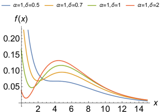
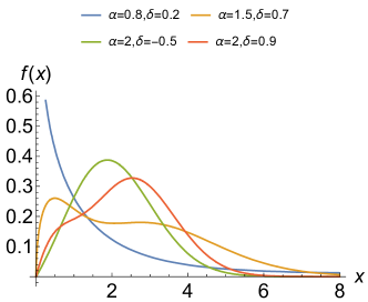
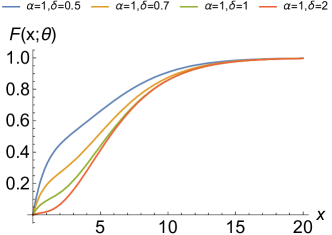
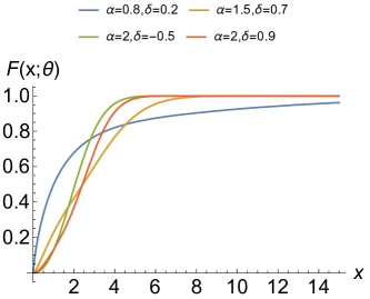
The p.d and c.d. functions (PDF and CDF) in Figures 1 and 2 are drawn for different values of parameters.
III Unimodality and Bimodality properties
Proposition III.1.
A point is a mode of the BWeibull density (1), if and only if it is a solution of the following equation
| (3) |
Proof.
The proof is trivial and omitted. ∎
Proposition III.2.
Proof.
The proof follows directly by applying Descartes’ rule of signs (see, e.g. Xue 2012 Xue2012 ). ∎
Proposition III.3 (Unimodality and monotonicity).
Let with . The following hold:
-
1)
If then the BWeibull density is unimodal;
-
2)
If then the BWeibull density is unimodal or strictly decreasing.
Proof.
Let . In this case note that the equation (3) can be written as
Firstly we assume that . By Descartes’ rule of signs the above equation has a unique positive root, denoted by . Since and we have that is the unique maximum point with maximum value . This proves the statement in the first item.
In the second case, , Descartes’ rule of signs guarantees that the equation has two roots, or zero roots. Since and , the proof of second item follows. ∎
Let us define
| (4) | ||||
the discriminant of the quartic polynomial , where
| (5) |
Theorem III.4 (Bimodality and unimodality).
Proof.
Let be a mode of the BWeibull density. By Proposition III.1 this mode satisfies the equation (3), with , or equivalently this one is solution of the quartic equation
with real coefficients defined in (5). By using that , in both cases, or (in this case, ), Descartes’ rule of signs guarantees that:
| (6) |
To check Items 1), 2) and 3), we first define the following quantities:
1) If then either the equation’s four roots are all real or none is. Since and whenever and , respectively, then all four roots of are real and distinct. Then, from affirmation (6) it follows that the equation has three distinct positive roots, denoted by , and one negative root. Let’s assume that . Since we have that and are two maximum points and is the unique minimum point. This proves the bimodality property in the first item.
2) If then the equation has two distinct real roots and two complex conjugate non-real roots. Then, from (6) it follows that the equation has one positive root, denoted by , and one negative root. Since , it follows that is the unique maximum point. This proves the second item.
3) If then the polynomial has a multiple root. Since and when , there are a triple root and a simple root, all real. Then, by affirmation (6), the equation has a positive triple root, denoted by , and one negative root. Since we have that is the unique maximum point. This completes the proof of third item. ∎
IV Characteristics of Probability Denstiy Function
IV.1 Real moments
Proposition IV.1.
If then
where is the complete gamma function.
Proof.
A simple observation shows that
where and is as in (2). By using the following formula of Item (6) in Cankaya2018 :
we have
By combining the above identities, the proof follows. ∎
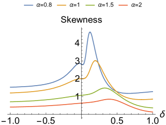
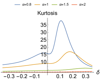
As a consequence of the above proposition, the closed expressions for the moments, variance, skewness and kurtosis of random variable are easily obtained. The Figures 3(a) and 3(b) give the skewness and kurtosis for the different values of bimodality parameter , respectively. For the tried values of and , we observe that when the value of are not large, we get a large scale of skewness and kurtosis. The Figure 3 represents that the parameter increases the flexiblity of function.
IV.2 Moment generating function
Theorem IV.2.
If then the moment generating function can be expressed as
Proof.
Using the series expansion of we have
Assuming the validity of the following identity
| (7) |
note that by using Proposition IV.1 and the identity , for (in the case ); the proof of the proposition follows.
In what remains of the proof we prove the identity (7). Indeed, from Monotone Convergence Theorem knapp we have
| (8) |
where, by Proposition IV.1, the series is written as
| (9) |
Note that the series defined by
converges when , because by the ratio test the limit
is less than 1 when ; and .
Corollary IV.3 (Light-tailed distribution).
If and , then there exists such that for large enough.
Proof.
Remark IV.4.
Let a continuous random variable with density function . Following the reference Klugman1998 , the rate of a random variable is given by
A simple computation shows that
Then, far enough out in the tail, every BWeibull distribution looks like an exponential distribution when and a Normal distribution when . In addition, we have some comparisons between the rates of random variables with known distributions: Inverse-gamma, Log-normal, Generalized-Pareto, BWeibull, BGamma Vila2020 , exponential and Normal;
By using the very well-known relation between moment generating function and characteristic function of , the following result follows immediately.
Proposition IV.5.
If then the characteristic function can be expressed as
IV.3 Reliability, hazard rate and the mean residual life
For any , the reliability, the hazard rate and the mean residual life functions, associated with a random variable , are defined as follows
respectively.
Let be a random variable with Weibull distribution. By using the integration by parts formula we have
By taking the change of variable the right-hand expression above is
where , , is the upper incomplete gamma function, and where we are adopting the notation . Therefore,
| (10) |
Similarly we find that
| (11) |
where , , is the lower incomplete gamma function.
Remark IV.6.
Proposition IV.7.
If then
-
1)
-
2)
-
3)
-
4)
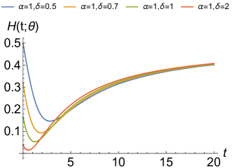
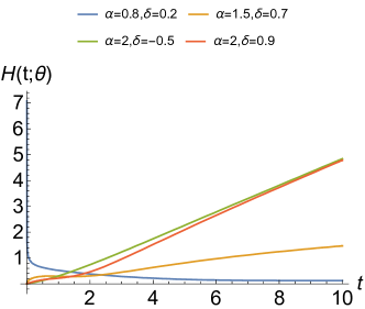
The hazard function in Figure 4 is drawn for different values of parameters.
Proof.
A simple algebraic manipulation in the definition of BWeibull density in equation (1) shows that
where is as in (2). By taking in (10), we get the formula of Item 1). By taking in (11), the formula of Item 2) follows. The proof of Item 3) follows immediately by combining the definition of with Item 1). The proof of Item 4) follows directly by analyzing the form of the hazard function in Item 3) through the known limits , , and standard limit calculations. ∎
Proposition IV.8.
If then
Proof.
Proposition IV.9 (Mean residual life function).
If then
IV.4 Entropies for continuous measure
The Tsallis Tsallis1988 , Quadratic Rao2010 and Shannon Shannon1948 entropies associated with a non-negative random variable are defined by
| (12) | ||||
| (13) | ||||
| (14) |
respectively.
Theorem IV.10 (Tsallis entropy).
Let and
where is the generalized binomial coefficient and . If and , then the Tsallis entropy is given by
Proof.
By definition of Tsallis entropy (12) note that it is enough to prove that
| (15) |
whenever , where is the normalization constant in equation (2).
Indeed, since
by using the Newton’s generalized binomial theorem the above integral is
where the condition guarantees that , and therefore the convergence of the above series. Seeing that (hypothesis), by Fubini’s theorem knapp the above integral is
| (16) |
where in the second equality we have used the classic binomial expansion. By using the formula of Item (6) in Cankaya2018 :
the expression in (IV.4) is rewritten as
whenever . Therefore, combining the above identities we have proved that the statement in (15) is valid. This completes the proof of theorem. ∎
Theorem IV.11 (Quadratic entropy).
Let . If then the quadratic entropy can be written as
Proof.
A simple algebraic manipulation shows that
where is as in (2). By using the formula of Item (6) in reference Cankaya2018 :
we have
where
Therefore,
Finally, taking logarithms to both sides of the above equation and then multiplying by , by definition (13) of quadratic entropy and by standard algebraic manipulations, we complete the proof.
∎
Let . By taking the change of variable , for each , we have
Since
the expectation can be written as follows
| (17) |
where is the the polygamma function of order .
Proposition IV.12.
If then
where is the Euler-Mascheroni constant.
Proof.
Through a simple calculation we have
Then, by taking in (17), from the above identity, the statement of proposition follows. ∎
Theorem IV.13 (Shannon entropy).
Let , , , for , and . If
then the Shannon entropy can be written as
Proof.
The Shannon entropy formula for the random variable , as defined in 14, is given by
Developing the logarithm in the above identity, we have
| (18) |
where and are given in Propositions IV.12 and IV.1, respectively.
It is worth mentioning that the expectation cannot be expressed through known mathematical functions. To obtain an expression for we consider Taylor’s expansion of the function around the point . Hence
| (19) |
Taking expectation on both sides of (19) we get
| (20) |
Since and (hypothesis), by applying Fubini’s Theorem knapp , the expression on the right-hand side of (20) is
By using binomial expansion repeatedly in the above expression, this is
Therefore, we get
| (21) |
V Inference: Estimation Methods and Fisher information
V.1 Maximum likelihood estimation method
Maximum likelihood estimation (MLE) method is the standard approach for estimations of parameters of , mainly due to the desirable asymptotic properties of consistency, efficiency and asymptotic normality Fer196 ; Fer296 .
The log likelihood function for is given by
| (22) | ||||
where is as in (2) and , , is the log likelihood function for the parameter vector .
A standard calculation shows that the first-order partial derivatives of are
| (26) |
where
and
Here, is the the polygamma function of order .
The second-order partial derivatives of can be written as
where
and
| (33) |
V.2 Maximum likelihood estimation method
The generalization of MLE with form is defined as maximum likelihood estimation (MLqE). is -deformed logarithm of natural logarithm () in MLE Tsallisbook09 . The concavity property of guarantees to replace in MLE by Lindsay94 ; CanKor18 ; Jan1 ; Jan2 .
| (34) |
where . If , then we have and so equation (22) is dropped. When likelihood is compared with likelihood, the deformation gives an advantage to manage the modelling capability of a parametric model. as an objective or loss function in MLqE in the M-estimation is used to manage efficiency and robustness for contamination. Note that is M-function MLqEBio ; CanKor18 . This estimation method is applied to BWeibull.
The function in equation (34) is optimized according to parameters in order to get the estimators of . Alternatively, a system of estimating equations can be solved simultaneously according to the corresponding estimating equation for the parameters , and . We omit to rewrite the system . Note that is given by equation (26) (with ) for and .
V.3 Fisher information based on and
Fisher information matrix (FI) is given by
| (35) |
and it is a tool to provide the variances of , i.e., Var(). As it is well-known, the inverse of FI gives Var() if the inverse of FI matrix exists Fisher25 ; LehmannCas98 . If the FI matrix is singular, then the generalized inverse techniques are used to get the inverse of FI even though we have information loss due to the used generalized inverse LiYeh12gen .
FI matrix based on is given by the following form:
| (36) |
where is sample size. is integral for partial derivatives of according to parameters and it is taken over probability density function . The subscript in represents second-order partial derivatives of according to parameters and . In other words, if then
where , , are given in Item (33) and
| (37) | ||||
| (38) | ||||
where is the Euler-Mascheroni constant, and
| (39) |
The proofs of equations (37)-(39) are followed by the integral kernel given by item (6) Cankaya2018 and taking derivative of both sides of integral or the software Mathematica 12.0 can be used.
The definition of Fisher information based on is given by, see Plastinoetal97 ; CanKor18 ,
| (40) |
where and is a parametric model. The calculation of integral is performed for one variable case from observations . Since it is replicated for case, FI matrix can be rewritten as the form in equation (36). If in equation (40), then drops to in equation (36). The connection between Fisher information and Tsallis -entropy is proved by CanKor18 . Since the analytical tractability of integral calculation cannot be easy to follow, the numerical integration technique in Mathematica 12.0 is used to get the values of elements in matrix in equation (40).
VI Application on real data sets
The real data sets are modelled by using BWeibull and BGamma distributions which have bimodality property. The parameter that gives an advantage to model the bimodal data which can occur due to contamination or irregularity into underlying or main distribution as an indicator for abnormalization in the working principle of a phenomena in the universe is used in Weibull and Gamma distributions. As it is clearly observed, the parameter with produces a modality due to fact that the function is polynomial with order . We confine ourself the real data sets which can be modelled by function having the bimodality property.
MLE and MLqE methods are used to estimate the model parameters. If a data set has two peaks, then it is expected that BWeibull and BGamma distributions capture the peaks and so they are flexible when they are compared with Weibull and Gamma distributions. Since BWeibull and BGamma distributions have analytical expression for their CDF, it is advantegous to use them for getting statistics from Kolmogorov-Smirnov (KS) and Cramér–von Mises (CVM). Since we use and in MLE and MLqE methods for getting the estimates of parameters, using information criteria (IC) such as Akaike and Bayesian, etc is not appropriate in view of the fact that and are not comparable. As it is well-known Hamparsum87 , the lack of fit part of IC depends on . There should be an equilibrium among the values of IC applied to different probability density functions. Since there does not exist have the equilibrium between and to make a comparison for lack of fit part of IC, it is not appropriate to use IC and we consult goodness of fit tests which are KS and CVM in order to test the modelling competence of the used objective functions produced by and God60 ; Hub64 as objective functions from MLE and MLqE, respectively. Note that MLE and MLqE are methods used to estimate the parameters of . However, are alternative step for calculation in order to reach the estimators from MLE. This alternative situation is a way to generalize MLE method as M-estimation method God60 ; Hub64 . in is a parameter to derive the different forms of Bercher12a . For this reason, likelihood and its special form ( likelihood) are applied to estimate the parameters .
The functions in equations (22)-(34) are nonlinear and the estimating equations for the parameters and are also nonlinear to get the estimators and analytically. The stochasticity and metaheuristic algorithms are tools used to optimize the nonlinear functions according to the parameters to get the estimates of and . The optimization of functions in equations (22)-(34) is performed by a ’metaheuristicOpt’ package with ’metaOpt’ function in free statistical software version . The chosen algorithm in ’metaOpt’ is Harmony Search (HS) harmony due to fact that we have the highest p-values of KS and CVM, which can show that BWeibull and BGamma with and should be optimized by ’metaOpt’ with HS. After applying the ’metaOpt’ with HS to functions in equations (22) and (34), we have the estimated values of from and likelihood estimaton methods. The parameter in likelihood estimation method is chosen according the biggest values of probability (p-value) for KS and CVM test statistics. Note that the objective function takes different forms for each value of . Thus, for only one parametric model , we can have neighborhoods of for different value of , which helps us to manage the efficiency and robustness while performing the modelling on data.
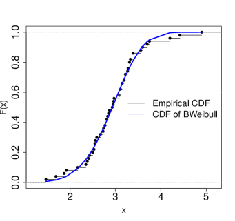
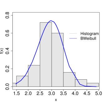
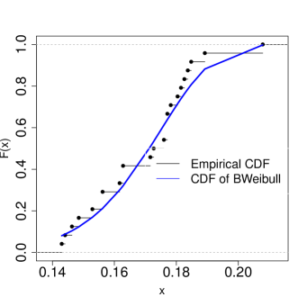
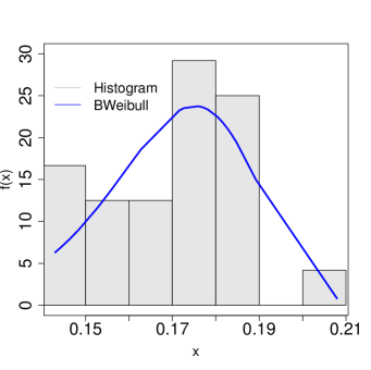
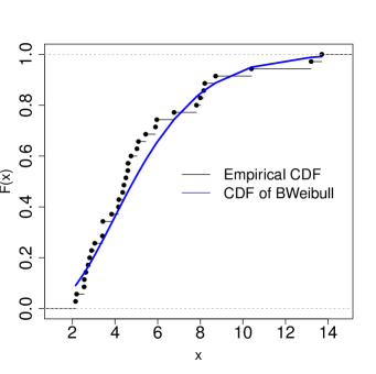
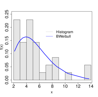
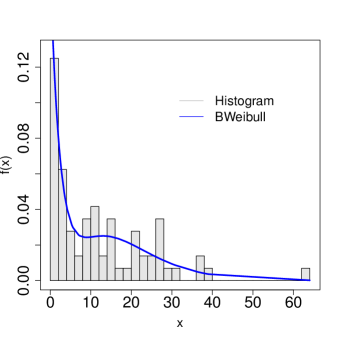
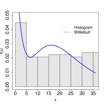
BWeibull and BGamma distributions with their , forms, i.e., and as objective functions are applied at real data sets in order to test the modelling competence on the data sets. The c.d. and p.d. functions abbreviated as CDF and PDF are superimposed on the empirical c.d. function and histogram of data to depict the best modelling chosen according to the p-values of KS and CVM (see Figures 5-9). In Figures 5(a)-9(a), CDF is more accurate illustration to depict the modelling of function with estimates and also the illustrations of CDF and PDF from Figures 5-9) show that the modelling on data sets is accomplished well. Using the probability values of KS and CVM is necessary to provide the homogenity for comparison with their corresponding test statistics of KS and CVM.
Example 1 : The data are the breaking stress of carbon fibers. First 10 subgroups in control which consists of observations are modelled by using Weibull distribution carbonfibers . Table 1 represents the values of estimates for the carbon fibers data modelled by BWeibull and BGamma with and as objective functions. The role of MLqE is observed. That is, there is an important increasing on the modelling competence when from MLqE is used. Note that it is observed that there is a good accommodation between this data as an empricial distribution and from MLqE, which can lead to have the highest p-value of KS. The parameter as tuning constant produces the neighborhoods of a parametric model, i.e., objective function, in order to increase the modelling competence of a parametric model Bercher12a .
| Model | KS | p-value(KS) | CVM | p-value(CVM) | |||
|---|---|---|---|---|---|---|---|
| BWeibull() | 3.6961(0.0807) | 2.7482(0.0306) | 2.3073(1.2630) | 0.14 | 0.7112 | 0.0690 | 0.1556 |
| BWeibull(), | 4.8707(0.1450) | 2.8434(0.0378) | 1.8986(2.4058) | 0.06 | 1 | 0.0158 | 0.1641 |
| BGamma() | 14.9970(0.6521) | 5.8832(0.2449) | 1.5823(1.0677) | 0.12 | 0.8643 | 0.0734 | 0.1549 |
| BGamma(), | 14.9994(0.7332) | 5.9217(0.3195) | 1.7915(3.0210) | 0.10 | 0.9639 | 0.0706 | 0.1553 |
KS: Kolmogorov-Smirnov, CVM: Cramér–von Mises, Bold represents the best fitting.
Example 2 : The data are maximum ozone concentrations labeled as ”o3max” in ”goft” package in free statistical software version . 24 observations are included by o3max. Table 2 shows MLE and MLqE with BWeibull are better than that of BGamma for the p-values of KS and CVM. Note that BWeibull with and has an important fitting competence when compared with that of BGamma.
| Model | KS | p-value(KS) | CVM | p-value(CVM) | |||
|---|---|---|---|---|---|---|---|
| BWeibull() | 10.0851(0.7039) | 0.1728(0.0018) | 14.9983(10.9941) | 0.1667 | 0.8928 | 0.0556 | 0.1577 |
| BWeibull(), | 10.1609(0.7079) | 0.1728(0.0018) | 14.9995(11.1710) | 0.1667 | 0.8928 | 0.0556 | 0.1577 |
| BGamma() | 3.2524(0.2537) | 14.9963(1.0863) | 1.6134(1.0448) | 0.4583 | 0.0129 | 0.6667 | 0.0856 |
| BGamma(), | 3.2513(0.2542) | 14.9935(1.0867) | 1.6130(1.0585) | 0.4583 | 0.0129 | 0.6667 | 0.0856 |
Example 3 : Growth hormone data was also modelled by Alizadeh . The number of observation is 35. MLqEs with BWeibull and BGamma distributions outperform when compared with parametric model in Alizadeh .
| Model | KS | p-value(KS) | CVM | p-value(CVM) | |||
|---|---|---|---|---|---|---|---|
| BWeibull() | 1.1344(0.0370) | 2.1303(0.1213) | 3.8210(1.0365) | 0.1429 | 0.8674 | 0.0651 | 0.1562 |
| BWeibull(), | 1.2489(0.0548) | 2.2989(0.1541) | 3.5132(1.4327) | 0.0857 | 0.9995 | 0.0357 | 0.1608 |
| BGamma() | 1.9136(0.1685) | 0.7620(0.0319) | 3.6132(1.7301) | 0.1429 | 0.8674 | 0.0765 | 0.1544 |
| BGamma(), | 2.4648(0.2891) | 0.9224(0.0513) | 3.2896(2.9941) | 0.0857 | 0.9995 | 0.0349 | 0.1610 |
Italic represents comparison for the best fitting for MLE of BWeibull and BGamma.
Table 3 represents the values of estimates for growth hormone data modelled by objective functions. Italic represents comparison between CVM values when MLE method is used. Note that MLE method reflects directly parametric models for which BWeibull and BGamma are used. In other words, deformation on the parametric model does not exist when we compare with . When MLEs of parameters of BWeibull and BGamma are compared, we observe that MLE of parameters of BWeibull is a little ahead for the performance of the fitting competence according to the values of CVM and its corresponding p-values. KS statistic and the corresponding p-values are not capable to assess the modelling competence. According to the values of p-value(CVM), MLqE with BGamma give the best performance on the modelling data when compared with MLqE with BWeibull.
Example 4 : Wheaton River data are analyzed by Vila2020 and references therein. The number of observation is 72. MLqE with BWeibull give outperforming when we compare by MLqE with BGamma. BGamma from Vila2020 has a good performance for fitting among the distributions Ortega11 and references therein. The advantage of using MLqE is observed when we look at the p-values of KS and CVM in Table 4.
| Model | KS | p-value(KS) | CVM | p-value(CVM) | |||
|---|---|---|---|---|---|---|---|
| BWeibull() | 0.9721(0.0102) | 5.4258(0.1397) | 0.1924(0.0050) | 0.0694 | 0.9951 | 0.0260 | 0.1624 |
| BWeibull(), | 0.9770(0.0103) | 5.4536(0.1411) | 0.1910(0.0050) | 0.0694 | 0.9951 | 0.0206 | 0.1633 |
| BGamma() | 1.0591(0.0182) | 0.1768(0.0023) | 0.1776(0.0039) | 0.0833 | 0.9639 | 0.0336 | 0.1612 |
| BGamma(), | 1.0568(0.0184) | 0.1780(0.0024) | 0.1783(0.0040) | 0.0833 | 0.9639 | 0.0287 | 0.1620 |

Example 5: The death occurring due to cancer increases. Gastric cancer data consisting of 125 observations are the censored data because of the difficulty of observering the patients who can die in the progress of medical treatment of patients. If data are censored, then there exists a replication for some observations, which leads to bimodaliy for frequency. For this reason, we prefer to use this data set which will be modelled by BWeibull and BGamma with and as objective functions. Let us note that censoring designs censoring ; Ngcensoring can be originally regarded as an objective function Hampeletal86 ; MLqEBio ; PhDthesis ; CanKor18 ; Canorder20 used to fit a data set. Thus, using and is reasonable and can be chosen as BWeibull and BGamma. Table 5 shows that MLqE with BWeibull should be considered as good fitting performance assessed by p-value of KS even if p-value of CVM of BGamma with as a little ahead from others is the best one among them.
| Model | KS | p-value(KS) | CVM | p-value(CVM) | |||
|---|---|---|---|---|---|---|---|
| BWeibull() | 1.1181(0.0092) | 8.4517(0.1373) | 0.1764(0.0031) | 0.104 | 0.5085 | 0.0962 | 0.1514 |
| BWeibull(), | 1.0092(0.0097) | 6.7659(0.1403) | 0.2106(0.0043) | 0.096 | 0.6121 | 0.1390 | 0.1450 |
| BGamma() | 0.9531(0.0133) | 0.1433(0.0030) | 0.2193(0.0031) | 0.112 | 0.4131 | 0.0849 | 0.1531 |
| BGamma(), | 0.9439(0.0147) | 0.1481(0.0012) | 0.2225(0.0036) | 0.104 | 0.5085 | 0.1422 | 0.1446 |

Conclusions
A bimodal form of Weibull distribution has been derived. The properties such as unimodality, bimodality, moment, moment generation functions, entropies, etc. have been obtained. In order to get the estimators of parameters, MLE and MLqE methods have been used. The concavity property of and are very important to apply for estimation of parameters Lindsay94 . Further, it should be noted that the existences of Shannon and Tsallis -entropies can also be important to apply MLE and MLqE methods. The estimates of from MLE and MLqE are obtained by using of the heuristic algorithm because of nonlinearity of and . The p.d. function has been chosen as BWeibull and BGamma distributions. Instead of using a parametric model directly for modelling a data set via , it should be preferred to apply which can derive the different forms of a parametric model for the different values of from MLqE method. Thus, we have obtained the results from numerical experiments showing that using MLqE method for parameters of BWeibull distribution is suggested. The anaytical expressions for the elements of FI based on have been obtained. The square root of variance values of estimators from MLE and MLqE are given in the numerical experiments.
The application of the proposed distribution for case of the censored data will be studied and comparative study for different forms of the censoring designs censoring ; Ngcensoring will be applied to test performance of the censoring designs when we have the empirical distribution which has bimodality. The properties such as existence, uniqueness of roots for and likelihood functions of the censoring designs which can be regarded as objective function Hampeletal86 will be studied.
Acknowledgments
This study was financed in part by the Coordenação de Aperfeiçoamento de Pessoal de Nível Superior - Brasil (CAPES) - Finance Code 001.
Appendix: Main buildings of codes used for computation of parameters and goodness of fit test statistics
The PDF is computed by
biwblpdf<- function(x,a,b,d){
Ψf=dweibull(x, a, b, log = FALSE);
ΨZ = 2 + ((2 *b *d *(-gamma(1/a) + b *d* gamma(2/a)))/a);
Ψg=(1 + (1 - d*x)^2)*f/Z;
}
The optimization of in equation (34) is performed by following functions:
ΨlogqLikFun <- function(p) {
ΨΨa <- p[1]; b <- p[2]; d <- p[3];
ΨΨ-sum((biwblpdf(x,a,b,d)^(1-q)-1)/(1-q))
Ψ}
Ψmlqe <- metaOpt(logqLikFun, optimType = "MIN", algorithm = "HS",
ΨnumVar,rangeVar,control = list(), seed = NULL)
The CDF arranged by manipulation and adopted for the computation of R platform is computed by
ΨCDFbiWei<- function(x,a,b,d){
ΨΨx=sort(x);
ΨΨG=(-2 * b * d * gamma(1/a) + a * (2 - 2 * exp(-(x/b)^a) +
ΨΨb^2 * d^2 * gamma(2/a+1) +   2 * b * d * (gamma(1 + 1/a)
ΨΨ* pgamma((x/b)^a, 1 + 1/a, 1, lower = FALSE))
ΨΨ- b^2 * d^2 * (gamma(2/a+1) * pgamma((x/b)^a, 2/a+1, 1, lower = FALSE))))
ΨΨ/(a * (2 + (2 * b * d * (-gamma(1/a) + b * d * gamma(2/a)))/a))
Ψ}
The values of goodness of fit test statistics are obtained by r1 ; r2
Ψinstall.packages("CDFt")
Ψlibrary("CDFt")
Ψval_CDFbiWeiq=CDFbiWei(sort(x),mleBiWeiabq[1],mleBiWeiabq[2],mleBiWeiabq[3])
Ψfun.ecdf=ecdf(x);my.ecdf <- fun.ecdf(sort(x));
Ψks.test(my.ecdf, val_CDFbiWeiq,alternative = c("two.sided", "less", "greater"),
Ψexact = NULL, tol=1e-8,simulate.p.value=FALSE,B=2000)
Ψresq = CramerVonMisesTwoSamples(my.ecdf,val_CDFbiWeiq);
ΨpvalueCVMq = 1/6*exp(-resq);
References
References
- (1) Ahsanullah, M., Hamedani, G. G. (2010). Exponential distribution: theory and methods. Nova Science Publ.
- (2) Castellares, F., Lemonte, A. J. (2015). A new generalized Weibull distribution generated by gamma random variables. Journal of the Egyptian Mathematical Society, 23(2), 382-390.
- (3) Xie, M., Tang, Y., Goh, T. N. (2002). A modified Weibull extension with bathtub-shaped failure rate function. Reliability Engineering & System Safety, 76(3), 279-285.
- (4) Martinez, E. Z., Achcar, J. A., Jácome, A. A., Santos, J. S. (2013). Mixture and non-mixture cure fraction models based on the generalized modified Weibull distribution with an application to gastric cancer data. Computer methods and programs in biomedicine, 112(3), 343-355.
- (5) Yang, G. (2007). Life cycle reliability engineering. John Wiley & Sons.
- (6) Silva, G. O., Ortega, E. M., Cordeiro, G. M. (2010). The beta modified Weibull distribution. Lifetime data analysis, 16(3), 409-430.
- (7) Rinne, H. (2008). The Weibull distribution: a handbook. CRC press.
- (8) Elal-Olivero, D. (2010). Alpha-skew-normal distribution. Proyecciones (Antofagasta), 29(3), 224-240.
- (9) Çankaya, M. N., Yalçınkaya, A., Altındaǧ, Ö., Arslan, O. (2019). On the robustness of an epsilon skew extension for Burr III distribution on the real line. Computational Statistics, 34(3), 1247-1273.
- (10) Çankaya M.N. Asymmetric bimodal exponential power distribution on the real line, Entropy, 2018, 20(1), 23.
- (11) Knapp, A. W. (2005). Basic real analysis. Springer Science & Business Media.
- (12) S. Klugman; H. Panjer; G. Willmot. Loss models: From data to decisions, Wiley, New York, 1998.
- (13) Rao C. R. Quadratic entropy and analysis of diversity, Sankhya A, 2010, 72, 70-80.
- (14) Shannon C.E. A mathematical theory of communication, Bell System Technical Journal, 1948, 27, 379-423, 623-656.
- (15) Tsallis C. Possible generalization of Boltzmann-Gibbs statistics, Journal of Statistical Physics, 1988, 52, 479-487.
- (16) Vila R.; Ferreira L.; Saulo H.; Prataviera F.; Ortega E. A bimodal gamma distribution: properties, regression model and applications, Statistics, 2020, 54(3), 469-493.
- (17) J. Xue. Loop Tiling for Parallelism, The Springer International Series in Engineering and Computer Science, Springer US, 2012.
- (18) Lindsay, B. G. (1994). Efficiency versus robustness: the case for minimum Hellinger distance and related methods. The annals of statistics, 22(2), 1081-1114.
- (19) C. Tsallis, Introduction to Nonextensive Statistical Mechanics: Approaching a Complex World, Springer, New York, 2009.
- (20) Ferguson, T. S. (1996). Strong Consistency of Maximum-Likelihood Estimates. In A Course in Large Sample Theory (pp. 112-118). Springer US.
- (21) Ferguson, T. S. (1996). Asymptotic Normality of the Maximum-Likelihood Estimate. In A Course in Large Sample Theory (pp. 119-125). Springer US.
- (22) Plastino, A., Plastino, A. R., Miller, H. G. (1997). Tsallis nonextensive thermostatistics and Fisher’s information measure. Physica A: Statistical Mechanics and its Applications, 235(3-4), 577-588.
- (23) Çankaya, M. N., Korbel, J. (2018). Least informative distributions in maximum q-log-likelihood estimation. Physica A: Statistical Mechanics and its Applications, 509, 140-150.
- (24) Geem, Z. W. (Ed.). (2009). Music-inspired harmony search algorithm: theory and applications (Vol. 191). Springer.
- (25) Sultan, K. S., Ismail, M. A., Al-Moisheer, A. S. (2007). Mixture of two inverse Weibull distributions: Properties and estimation. Computational Statistics Data Analysis, 51(11), 5377-5387.
- (26) Sultan, K. S., Al-Moisheer, A. S. (2013). Estimation of a discriminant function from a mixture of two inverse Weibull distributions. Journal of Statistical Computation and Simulation, 83(3), 405-416.
- (27) Hasegawa, Y., Arita, M. (2009). Properties of the maximum q-likelihood estimator for independent random variables. Physica A: Statistical Mechanics and its Applications, 388(17), 3399-3412.
- (28) Nichols, M. D., Padgett, W. J. (2006). A bootstrap control chart for Weibull percentiles. Quality and reliability engineering international, 22(2), 141-151.
- (29) Bozdogan, H. (1987). Model selection and Akaike’s information criterion (AIC): The general theory and its analytical extensions. Psychometrika, 52(3), 345-370.
- (30) Godambe, V. P. (1960). An optimum property of regular maximum likelihood estimation. The Annals of Mathematical Statistics, 31(4), 1208-1211.
- (31) Huber, P. J. (1964). Robust estimation of a location parameter: Annals Mathematics Statistics, 35.
- (32) Fisher, R. A. (1925, July). Theory of statistical estimation. In Mathematical Proceedings of the Cambridge Philosophical Society (Vol. 22, No. 5, pp. 700-725). Cambridge University Press.
- (33) E.L. Lehmann, G. Casella, Theory of point estimation, Wadsworth & Brooks/Cole. Pacific Grove, CA, 589, USA, 1998.
- (34) L. Pardo, Statistical inference based on divergence measures, CRC Press, Taylor & Francis Group, 2005.
- (35) Korbel, J., Hanel, R., Thurner, S. (2019). Information geometric duality of -deformed exponential families. Entropy, 21(2), 112.
- (36) Korbel, J., Hanel, R., Thurner, S. (2020). Information geometry of scaling expansions of non-exponentially growing configuration spaces. The European Physical Journal Special Topics, 229(5), 787-807.
- (37) Li, Y. H., Yeh, P. C. (2012). An interpretation of the Moore-Penrose generalized inverse of a singular Fisher Information Matrix. IEEE Transactions on Signal Processing, 60(10), 5532-5536.
- (38) Bercher, J. F. (2012). A simple probabilistic construction yielding generalized entropies and divergences, escort distributions and q-Gaussians. Physica A: Statistical Mechanics and its Applications, 391(19), 4460-4469.
- (39) Alizadeh, M., Bagheri, S. F., Samani, E. B., Ghobadi, S., Nadarajah, S. (2018). Exponentiated power Lindley power series class of distributions: Theory and applications. Communications in Statistics-Simulation and Computation, 47(9), 2499-2531.
- (40) De Pascoa, M. A., Ortega, E. M., Cordeiro, G. M. (2011). The Kumaraswamy generalized gamma distribution with application in survival analysis. Statistical methodology, 8(5), 411-433.
- (41) F.R. Hampel, E. M. Ronchetti, P. J. Rousseeuw, W. A. Stahel, Robust statistics: The approach based on influence functions, Wiley Series in Probability and Statistics, New York, 1986.
- (42) Çankaya, M. N. 2015. M-Estimators with asymmetric influence function: Properties and their applications. PhD diss., University of Ankara.
- (43) Çankaya, M. N. (2020). M-Estimations of Shape and Scale Parameters by Order Statistics in Least Informative Distributions on q-deformed logarithm. Iǧdır Üniversitesi Fen Bilimleri Enstitüsü Dergisi, 10(3), 1984-1996.
- (44) McCool, J. I. (2012). Using the Weibull distribution: reliability, modeling, and inference (Vol. 950). John Wiley & Sons.
- (45) Lio, Y., Ng, H. K. T., Tsai, T. R., Chen, D. G. (Eds.). (2019). Statistical Quality Technologies: Theory and Practice. Springer.
- (46) https://www.r-bloggers.com/2015/01/goodness-of-fit-test-in-r/, 09/17/2020
- (47) https://www.rdocumentation.org/packages/CDFt/versions/1.0.1/topics/CramerVonMisesTwoSamples, 09/17/2020