Spontaneous spatial order in two-dimensional ferromagnetic spin-orbit coupled uniform spin-1 condensate solitons

Abstract

We demonstrate spontaneous spatial order in stripe and super-lattice solitons in a Rashba spin-orbit (SO) coupled spin-1 uniform quasi-two-dimensional (quasi-2D) ferromagnetic Bose-Einstein condensate. For weak SO coupling, the solitons are of the $(-1,0,+1)$ or $(0,+1,+2)$ type with intrinsic vorticity, where the numbers in the parentheses denote angular momentum in spin components $F_{z}=+1,0,-1$, respectively. For intermediate SO coupling, three types of solitons are found: (a) circularly-asymmetric solitons, (b) circularly-symmetric $(-1,0,+1)$- and (c) $(0,+1,+2)$-type multi-ring solitons maintaining the above-mentioned vortices in respective components. For large SO coupling, quasi-degenerate stripe and super-lattice solitons are found in addition to the circularly-asymmetric solitons. A super-lattice soliton forms a 2D square lattice structure in the total density as in a super-solid; in component densities it may have either (i) a 1D stripe pattern or (ii) a 2D square lattice structure.

A super-solid [1] is a special quantum state where matter forms a stable, spatially-ordered structure, breaking continuous translational invariance, as in a crystalline solid, and has friction-less flow as in a super-fluid, breaking continuous gauge invariance. In other words, it possesses qualities of a super-fluid and a solid, in contradiction to the intuition that friction-less flow is a property exclusive to quantum fluids, e.g. Bose–Einstein condensate (BEC) [2], and Fermi super-fluid [3]. The search of a super-solid helium [4] was inconclusive [5]. It is possible to mimic a super-solid by an engineering with a external periodic potential in a super-fluid [6], e.g. using an optical-lattice potential. Following theoretical suggestions to create a super-solid with dipolar [7] and finite-range [8] atomic interactions, more recently, different experimental groups confirmed its presence in a dipolar BEC in quasi-two-dimensional (quasi-2D) [9] and quasi-one-dimensional (quasi-1D) [10] geometries.

There have also been suggestions to create a super-solid in a spin-orbit (SO) coupled spinor BEC [11, 12]. The SO coupling naturally appears in charged electrons and controls many properties of a solid including its crystalline or amorphous structure. Although, in a neutral atom, there cannot be a natural SO coupling, it is possible to introduce an artificial synthetic SO coupling by Raman lasers that coherently couple the spin-component states in a spinor BEC [13]. Two possible SO couplings are due to Rashba [14] and Dresselhaus [15]. An equal mixture of these SO couplings has been realized in pseudo spin-1/2 ⁸⁷Rb [16] and ²³Na [17] BECs containing only two spin components $F_{z}=0,-1$ of total spin $F=1$, and in a spin-1 ferromagnetic ⁸⁷Rb BEC, containing all three spin components $F_{z}=\pm 1,0$ [18]. A spin-1 spinor BEC [19] appears in two magnetic phases with distinct properties [20]: ferromagnetic $(a_{0}>a_{2})$ and anti-ferromagnetic $(a_{0}<a_{2})$, where $a_{0}$ and $a_{2}$ are the scattering lengths in the total spin 0 and 2 channels, respectively. Following theoretical suggestions [11, 21], recently, there has been experimental confirmation of a periodic one-dimensional (1D) super-stripe state with density modulation in an SO-coupled pseudo spin-1/2 spinor BEC [22] employing an equal mixture of Rashba and Dresselhaus couplings.

In this letter, we pursue a numerical study of the spin-1 quasi-two-dimensional (quasi-2D) Rashba SO-coupled uniform self-attractive ferromagnetic BEC using a mean-field model. For a weakly Rashba SO-coupled spin-1 BEC, two types of quasi-degenerate circularly-symmetric solitons are formed. The solitons are either of the $(-1,0,+1)$ type or of the $(0,+1,+2)$ type, where the numbers in parentheses represent the angular momentum of vortices at the center of components $F_{z}=+1,0,-1$ [23], the positive (negative) sign corresponds to a vortex (an anti-vortex). For medium SO-coupling, quasi-degenerate circularly-symmetric multi-ring solitons are formed maintaining the above-mentioned vortices at the respective centers in addition to circularly-asymmetric solitons without any internal vortex. The circularly-asymmetric solitons have the lowest energy and they continue to exist for larger strengths of SO coupling. For large SO coupling, the solitons develop spontaneous spatial order in the form of quasi-2D crystallization onto a square lattice in total density, sharing some properties of a super-solid, viz. Fig. 1 of Ref. [24], Fig. 1 of Ref. [12] and Fig. 1(e) of Ref. [21], breaking continuous translational symmetry, as in a super-solid, possessing either 1D stripe or quasi-2D crystallization in component densities and will be termed super-lattice solitons. The multi-ring, viz. Figs. 3(d)-(i), and stripe, viz. Figs. 4(d)-(f), solitons only exhibit a periodic structure in the component densities, due to a phase separation among the components without any periodic structure in the total density. A 2D super-solid crystalline phase was recently created in a ⁸⁷Rb BEC dispersively coupled with two optical cavities and illuminated by a 1D transverse pump lattice [25]. The present SO-coupled quasi-2D super-lattice soliton without any periodic potential in the Hamiltonian is different from this recently observed 2D super-crystal [25] formed in the presence of a self-consistent periodic potential generated from the interference between the transverse pump field and the two cavity fields. The present quasi-2D super-lattice state should serve as a laboratory model for crystallization in a solid in a controlled environment. A similar study in a normal solid is very limited due to impurities and lack of information about the interactions. There have been studies of quasi-1D [26], quasi-2D [27] and three-dimensional [28] solitons in pseudo spin-1/2 SO-coupled BEC and no super-lattice state has been reported there.

We consider a BEC of $N$ atoms, of mass $m$ each, free in the $x-y$ plane and under a harmonic trap $V({\bf r})=m\omega_{z}^{2}z^{2}/2$ in the $z$ direction with $\omega_{z}$ the angular trap frequency. Integrating out the $z$ coordinate [29], we have the single-particle Hamiltonian of the quasi-2D Rashba SO-coupled BEC as [16, 20]

$$H_{0}=-\frac{\hbar^{2}}{2m}\nabla_{\boldsymbol{\rho}}^{2}+\gamma\left[p_{y}\Sigma_{x}-p_{x}\Sigma_{y}\right],$$ (1)

where ${\boldsymbol{\rho}}\equiv\{x,y\}$, $\nabla_{\boldsymbol{\rho}}^{2}\equiv(\partial_{x}^{2}+\partial_{y}^{2})$, $\partial_{x}\equiv\partial/\partial x$, $\partial_{y}\equiv\partial/\partial y$, the $x$ and $y$ components of the momentum operator $p_{x}=-i\hbar\partial_{x},p_{y}=-i\hbar\partial_{y}$, $\gamma$ is the strength of Rashba SO coupling and the irreducible representation of the spin-1 spin matrices $\Sigma_{x}$ and $\Sigma_{y}$ are

$$\Sigma_{x}=\frac{1}{\sqrt{2}}\begin{pmatrix}0&1&0\\ 1&0&1\\ 0&1&0\end{pmatrix},\quad\Sigma_{y}=\frac{i}{\sqrt{2}}\begin{pmatrix}0&-1&0\\ 1&0&-1\\ 0&1&0\end{pmatrix}.$$ (2)

The reduced quasi-2D coupled Gross-Pitaevskii (GP) equations [29] of the three spin components, for the SO-coupled spin-1 spinor BEC, are [20]

$$i\partial_{t} \psi_{\pm 1}({\boldsymbol{\rho}})=\left[{\cal H}+{c_{2}}\left(n_{\pm 1}-n_{\mp 1}+n_{0}\right)\right]\psi_{\pm 1}({\boldsymbol{\rho}})$$

$$+ \left\{c_{2}\psi_{0}^{2}({\boldsymbol{\rho}})\psi_{\mp 1}^{*}({\boldsymbol{\rho}})\right\}-i{\widetilde{\gamma}}(\partial_{y}\pm i\partial_{x})\psi_{0}({\boldsymbol{\rho}})\,,$$ (3)

$$i\partial_{t} \psi_{0}({\boldsymbol{\rho}})=\left[{\cal H}+{c_{2}}\left(n_{+1}+n_{-1}\right)\right]\psi_{0}({\boldsymbol{\rho}})+\big{\{}2c_{2}\psi_{+1}({\boldsymbol{\rho}})$$

$$\times \psi_{-1}({\boldsymbol{\rho}})\psi_{0}^{*}({\boldsymbol{\rho}})\big{\}}{-i{\widetilde{\gamma}}[-i\partial_{x}\phi_{-1}({\boldsymbol{\rho}})+\partial_{y}\phi_{+1}({\boldsymbol{\rho}})]}\,,$$ (4)

$${\cal H}= -\frac{1}{2}\nabla^{2}_{\boldsymbol{\rho}}+c_{0}n,$$ (5)

$$c_{0}= \frac{2{N}\sqrt{2\pi}(a_{0}+2a_{2})}{3},\quad c_{2}=\frac{2{N}\sqrt{2\pi}(a_{2}-a_{0})}{3},$$ (6)

where $\widetilde{\gamma}=\gamma/\sqrt{2}$, $\partial_{t}\equiv\partial/\partial t$, $\phi_{\pm}({\boldsymbol{\rho}})=\psi_{+1}({\boldsymbol{\rho}})\pm\psi_{-1}({\boldsymbol{\rho}})$, $n_{j}=|\psi_{j}|^{2},j=\pm 1,0$ are the densities of spin components $F_{z}=\pm 1,0$, the total density $n({\boldsymbol{\rho}})=\sum_{j}n_{j}({\boldsymbol{\rho}})$, and the asterisk denotes complex conjugate. All quantities in Eqs. (Spontaneous spatial order in two-dimensional ferromagnetic spin-orbit coupled uniform spin-1 condensate solitons)-(6) are dimensionless, as we express lengths ($a_{0},a_{2},x,y,z$) in units of oscillator length $l_{0}\equiv\sqrt{\hbar/m\omega_{z}}$, density in units of $l_{0}^{-2}$, time in units of $\omega_{z}^{-1}$, and energy in units of $\hbar\omega_{z}$. The normalization condition is ${\textstyle\int}n({\boldsymbol{\rho}})\,d{\boldsymbol{\rho}}=1$. A spin-1 spinor BEC appears in two magnetic phases: ferromagnetic ($c_{2}<0$) and anti-ferromagnetic ($c_{2}>0$). The stationary solutions are governed by the time-independent version of Eqs. (Spontaneous spatial order in two-dimensional ferromagnetic spin-orbit coupled uniform spin-1 condensate solitons)-(Spontaneous spatial order in two-dimensional ferromagnetic spin-orbit coupled uniform spin-1 condensate solitons) with the energy functional

$$E[\psi] =\frac{1}{2}{\textstyle\int}d{\boldsymbol{\rho}}\big{[}{\textstyle\sum}_{j}|\nabla_{\boldsymbol{\rho}}\psi_{j}|^{2}-2\mu n+\rho^{2}n+c_{0}n^{2}$$

$$+c_{2}\big{\{}n_{+1}^{2}+n_{-1}^{2}+2(n_{+1}n_{0}+n_{-1}n_{0}-n_{+1}n_{-1}$$

$$\times+\psi_{-1}^{*}\psi_{0}^{2}\psi_{+1}^{*}+\psi_{-1}\psi_{0}^{*2}\psi_{+1})\big{\}}$$

$$-2i\widetilde{\gamma}\big{\{}\psi_{0}^{*}\partial_{y}\phi_{+}+\phi_{+}^{*}\partial_{y}\psi_{0}-i\psi_{0}^{*}\partial_{x}\phi_{-}+i\phi_{-}^{*}\partial_{x}\psi_{0}\big{\}}\big{]}+\mu,\qquad$$ (7)

where $\mu$ is the chemical potential. However, the numerical value of energy is independent of the chemical potential.

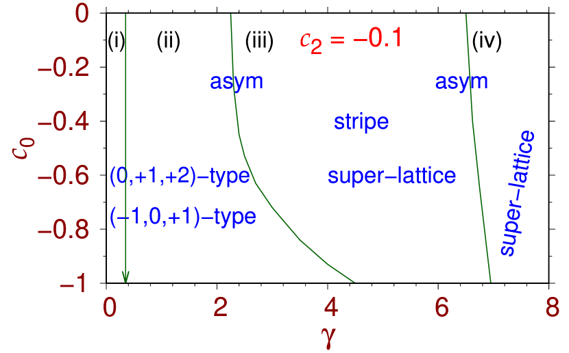
Figure 1: The $c_{0}$ versus $\gamma$ phase plot for Rashba SO coupling in different regions of parameter space: (i,ii)$(0,+1,+2)$ and $(-1,0,+1)$-type solitons; (ii,iii,iv) circularly asymmetric soliton; (iii) stripe and super-lattice solitons; (iv) super-lattice solitons. Results in all Figs. are in dimensionless units.

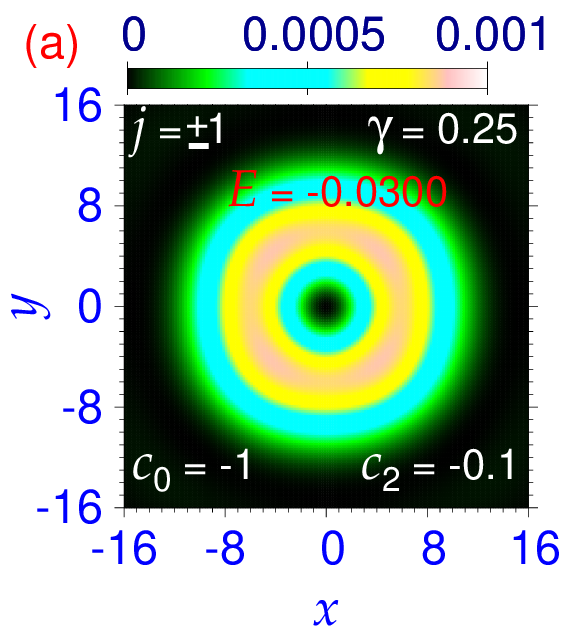
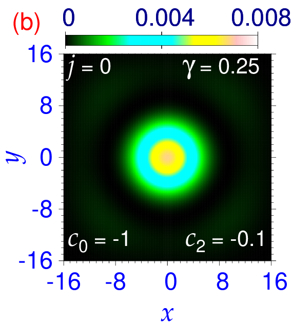
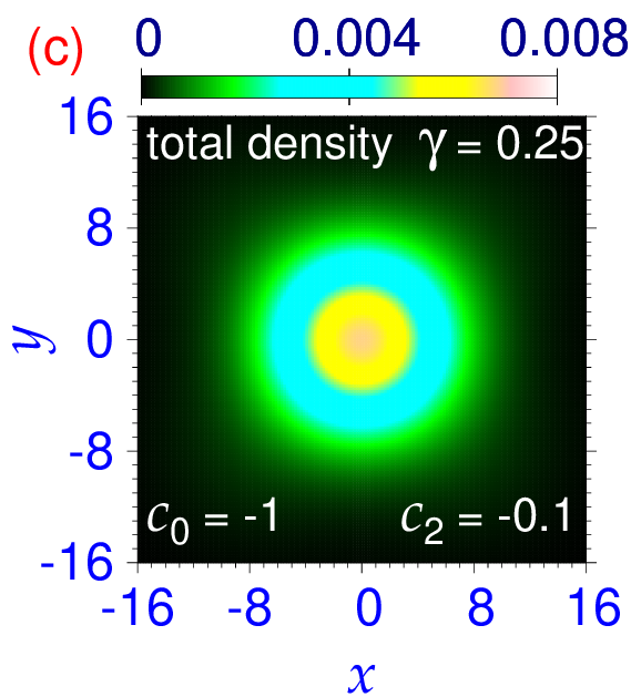
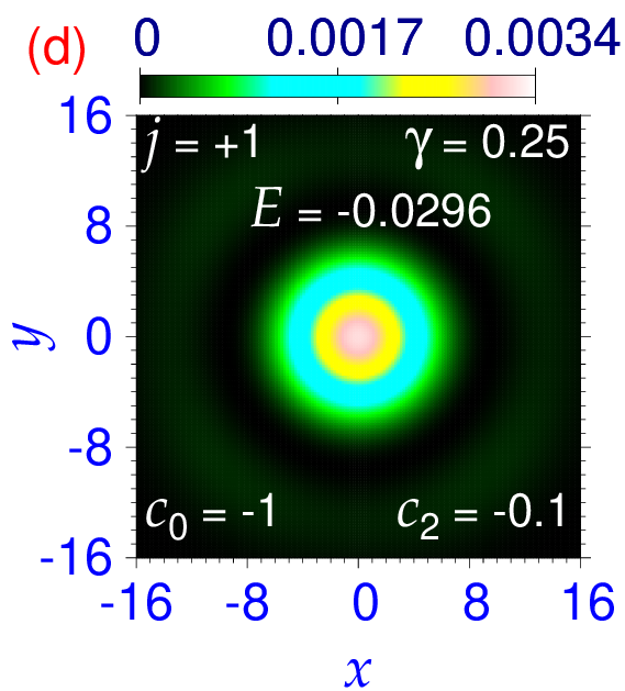
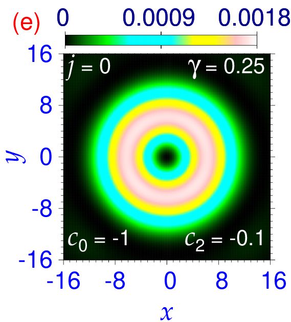
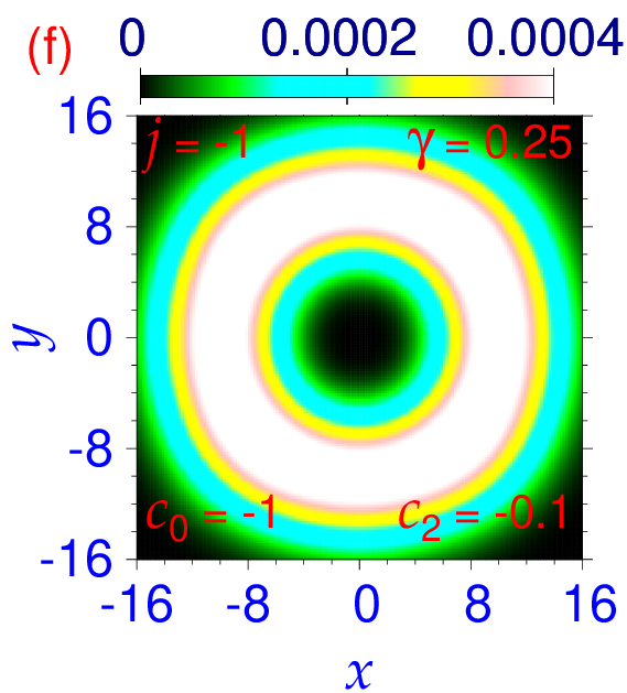
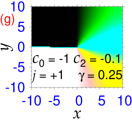
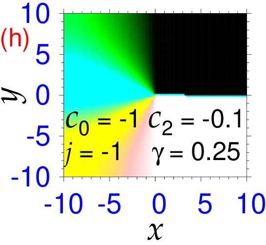
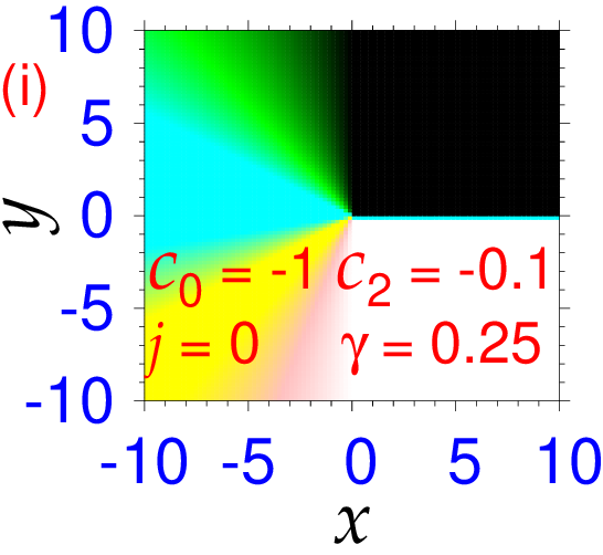
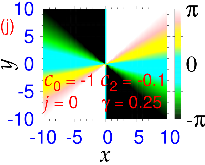
Figure 2: Contour plot of density $n_{j}(\boldsymbol{\rho})$ of components (a) $j=\pm 1$, (b) $j=0$ and (c) total density $n(\boldsymbol{\rho})$ of a $(-1,0,+1)$-type Rashba SO-coupled soliton for $c_{0}=-1,c_{2}=-0.1,\gamma=0.25$; the same of components (d) $j=+1,$ (e) $j=0$, (f) $j=-1$ of a $(0,+1,+2)$-type soliton; the phase of wave-function components (g) $j=+1$ and (h) $j=-1$ of the Rashba SO-coupled $(-1,0,+1)$-type BEC soliton; the phase of (i) $j=0$ and (j) $j=-1$ components of the Rashba SO-coupled $(0,+1,+2)$-type BEC soliton. The energies are displayed in the $j=+1$ component in Figs. 2-5.

We solve Eqs. (Spontaneous spatial order in two-dimensional ferromagnetic spin-orbit coupled uniform spin-1 condensate solitons) and (Spontaneous spatial order in two-dimensional ferromagnetic spin-orbit coupled uniform spin-1 condensate solitons) numerically propagating these in time by the split-time-step Crank-Nicolson discretization scheme [30] employing a space step of 0.1 and a time step of 0.001 and 0.00025, respectively, for imaginary- and real-time propagation. Imaginary-time propagation is used to find the lowest-energy soliton in different parameter domains. Real-time propagation is used to test the dynamical stability of the solution. Magnetization is not a good quantum number and evolves freely during time propagation to attain a final converged value.

To simulate a self-attractive ($c_{0}<0$) ferromagnetic ($c_{2}<0$) SO-coupled spinor BEC for different strengths of SO coupling $\gamma$, we consider a system with $c_{2}=-0.1$ and vary $c_{0}$ and $\gamma$ in this study. We consider $c_{0}$ in the range $0>c_{0}>-1$, as for $c_{0}<-1$, because of increased attraction, the soliton shrinks and its size becomes too small for a useful calculation. In Fig. 1 we illustrate the formation of different types of solitons for Rashba SO coupling via the phase plot of $c_{0}$ versus $\gamma$ for $c_{2}=-0.1$. Solitons of type $(-1,0,+1)$ and $(0,+1,+2)$ are formed in region (i) as well as (ii); in the second they evolve into multi-ring solitons. Circularly-asymmetric solitons are formed in regions (ii), (iii), and (iv). Super-lattice solitons are formed in regions (iii) and (iv). Stripe solitons are formed in region (iii).

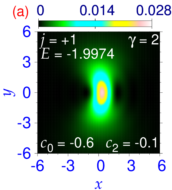
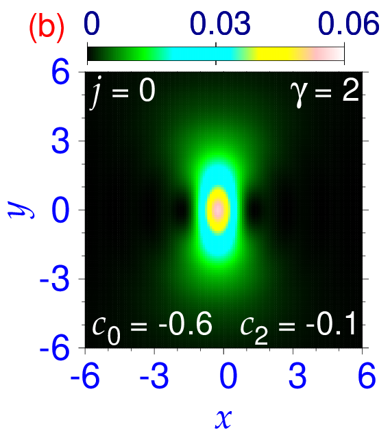
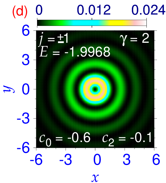
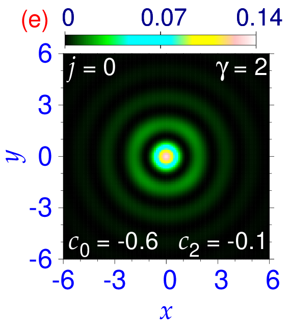
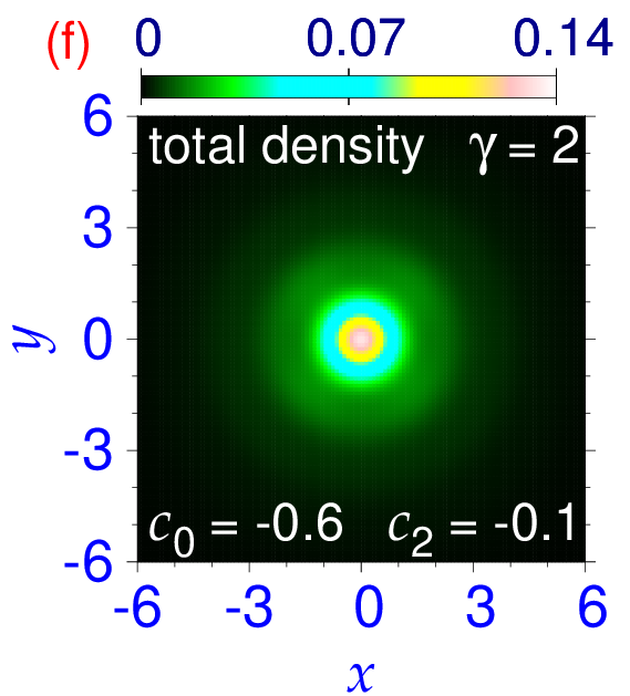
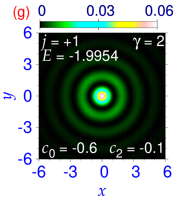
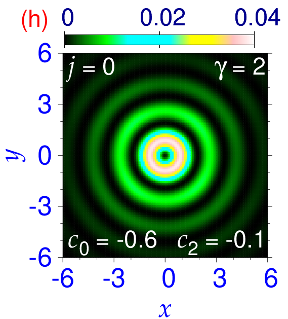
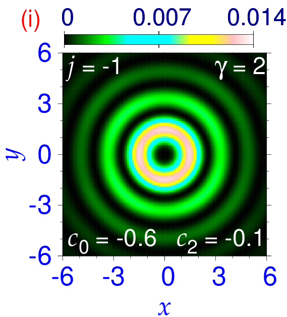
Figure 3: Contour plot of density $n_{j}(\boldsymbol{\rho})$ of wave-function components (a) $j=+1$, (b) $j=0$ and (c) $j=-1$ of the asymmetric Rashba SO-coupled soliton with $c_{0}=-0.6,c_{2}=-0.1,\gamma=2$; the same of the $(-1,0,+1)$-type soliton of components (d) $j=\pm 1$, (e) $j=0$, and (f) the total density $n(\boldsymbol{\rho})$; the same of the $(0,+1,+2)$-type soliton of components (g) $j=+1$, (h) $j=0$ and (i) $j=-1$.

First we consider a small SO-coupling strength ($\gamma=0.25$), where two quasi-degenerate vector solitons of type $(-1,0,+1)$ and $(0,+1,+2)$ are formed for Rashba SO coupling obtained by imaginary-time propagation using initial localized functions with the appropriate vortices imprinted in the respective components. In Figs. 2(a)-(c) we display the contour plot of density of components (a) $j=\pm 1$ and (b) $j=0$ and (c) total density of a $(-1,0,+1)$-type soliton for parameters $c_{0}=-1,c_{2}=-0.1,\gamma=0.25$. In Figs. 2(d)-(f) we show the same of components (a) $j=+1$ and (b) $j=0$ and (c) $j=-1$ of a $(0,+1,+2)$-type soliton for the same parameters. The energy of the $(-1,0,+1)$- and $(0,+1,+2)$-type solitons in Fig. 2 are $E=-0.0300$ and $E=-0.0296$ respectively. In Figs. 2(g)-(h) we display the contour plot of the phase of wave-function components $j=\pm 1$ of the $(-1,0,+1)$-type Rashba SO-coupled soliton of Fig. 2(a) showing a phase drop of $\mp 2\pi$ under a complete rotation, indicating angular momenta of $\mp 1$ in these components. In Figs. 2(i)-(j) we display the same of components $j=0,-1$ of the $(0,+1,+2)$-type Rashba SO-coupled soliton of Figs. 2(e)-(f) showing a phase drop of $2\pi$ and $4\pi$ under a complete rotation, indicating angular momenta of $+1$ and $+2$ in these components. The phases are consistent with the vortex (anti-vortex) structure of the $(-1,0,+1)$ and $(0,+1,+2)$-type solitons.

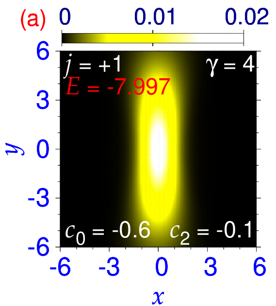
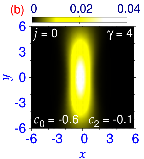
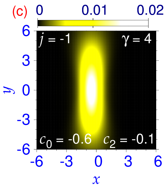
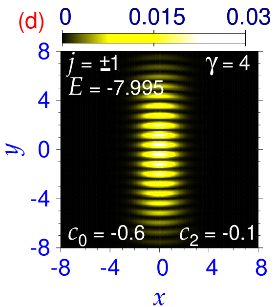
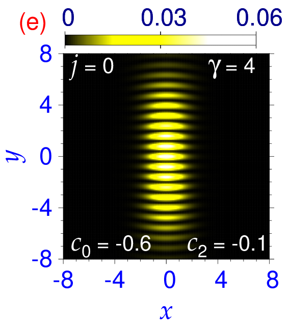
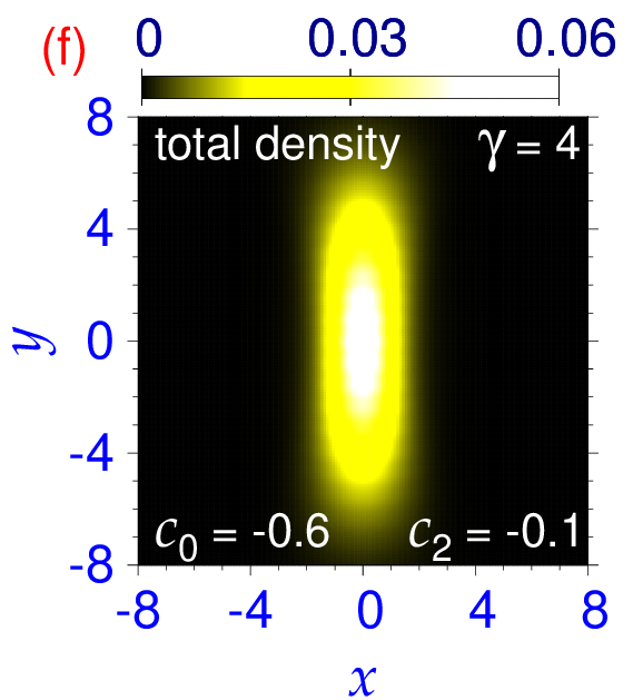
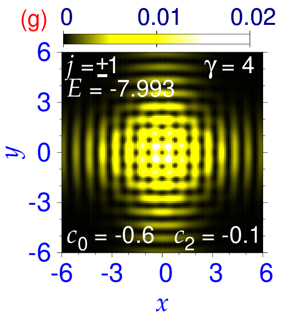
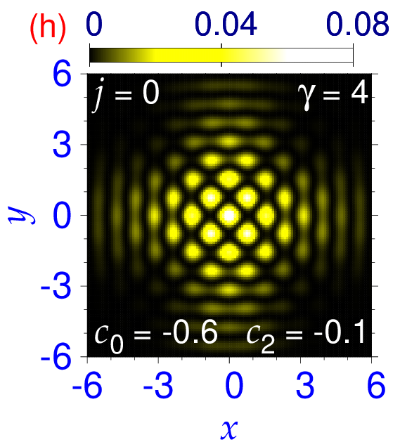
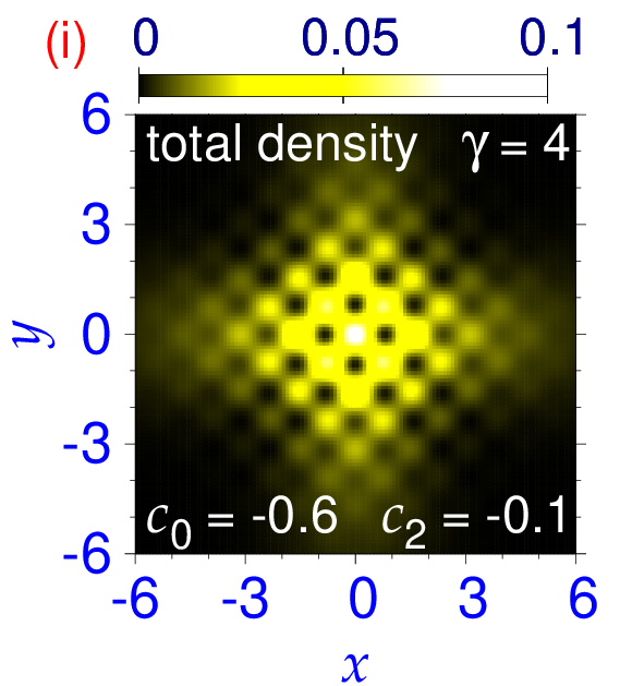
Figure 4: Contour plot of density $n_{j}(\boldsymbol{\rho})$ of components (a) $j=+1$, (b) $j=0$ and (c) $j=-1$ of the asymmetric Rashba SO-coupled soliton with $c_{0}=-0.6,c_{2}=-0.1,\gamma=4$; the same of components (d) $j=\pm 1$, (e) $j=0$, and (f) the total density $n(\boldsymbol{\rho})$ of the stripe soliton; (g)-(i) the same of the super-lattice soliton.

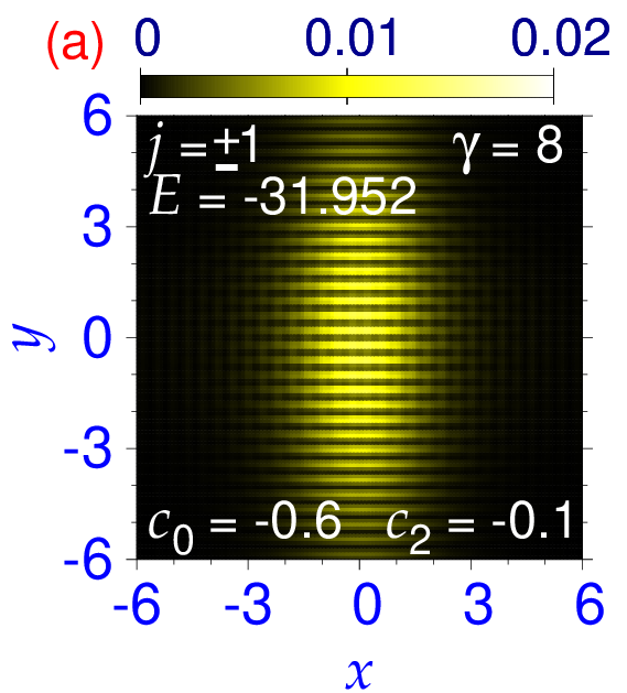
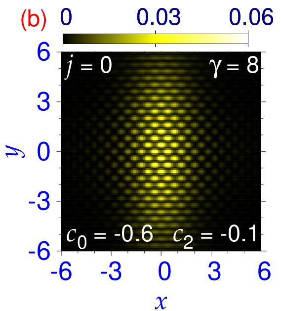
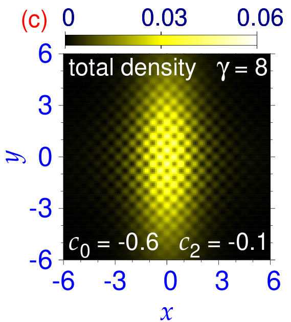
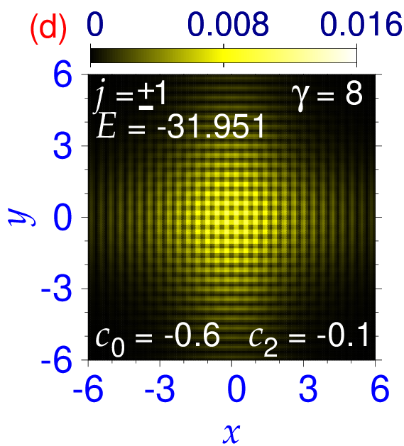
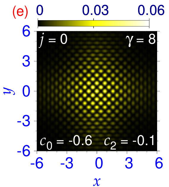
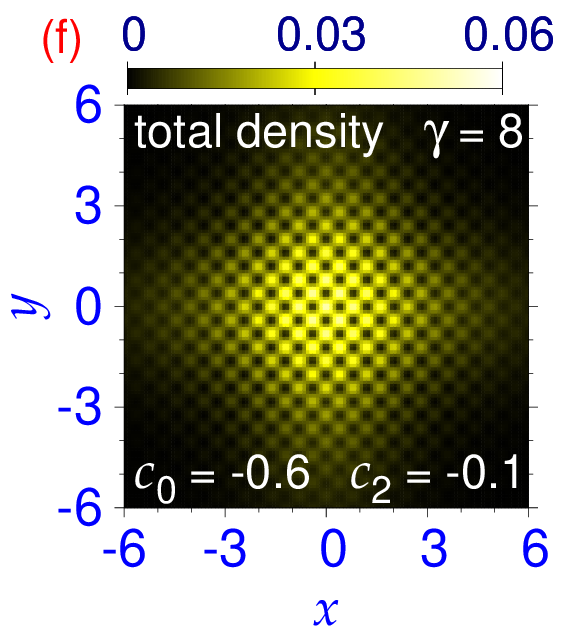
Figure 5: Contour plot of density $n_{j}(\boldsymbol{\rho})$ of components (a) $j=\pm 1$, (b) $j=0$ and (c) the total density $n(\boldsymbol{\rho})$ of the super-lattice Rashba SO-coupled soliton with stripe in components $j=\pm 1$ for $c_{0}=-0.6,c_{2}=-0.1,\gamma=8$; (d)-(f) the same of the super-lattice soliton with 2D square lattice formation in components $j=\pm 1$.

Three types of quasi-degenerate vector solitons are found as $\gamma$ is increased. In addition to the circularly-symmetric solitons an asymmetric soliton appears as the lowest-energy state, viz. Figs. 3(a)-(c) for $c_{0}=-0.6,c_{2}=-0.1$ and $\gamma=2$, illustrating the $j=+1,0,-1$ components, respectively. The $(-1,0,+1)$- and $(0,+1,+2)$-type solitons develop concentric radially-periodic rings around a central core maintaining the appropriate vortices in the respective components and become $(-1,0,+1)$- and $(0,+1,+2)$-type multi-ring solitons, as shown in Figs. 3(d)-(f) and (g)-(i), respectively. The phases of the wave-function components of the multi-ring solitons (not shown here) are identical to the same of the $(-1,0,+1)$- and ($0,+1,+2$)-type solitons of Figs. 2(g)-(j) reflecting the same vortex (anti-vortex) structure at the center of the respective components for Rashba SO coupling. The total density in all these solitons have a smooth distribution of matter as shown in Fig. 3(f) for the $(-1,0,+1)$-type multi-ring soliton. Of these three types of quasi-degenerate solitons, the circularly-asymmetric state of energy $E=-1.9974$ is the lowest-energy state. The first excited state is the $(-1,0,+1)$-type state with energy $E=-1.9968$; the next state is the $(0,+1,+2)$-type state with energy $E=-1.9954$. The increase of $\gamma$ from Fig. 2 to Fig. 3 has increased the binding, and hence aids in forming soliton. The change in binding due to the change of $c_{0}$ from Fig. 2 to Fig. 3 is negligible in this scale. Multi-ring solitons were also investigated in a quasi-2D pseudo spin-1/2 SO-coupled BEC trapped in a radially-periodic potential [31] which creates the multi-ring modulation in component densities due to the presence of the external radially-periodic trap. However, the present radial modulation in density without any external trap is a consequence of the Rashba SO coupling.

The single-particle Hamiltonian (1) should have solutions of the plane wave form $\exp(\pm i\alpha\gamma x)\otimes\exp(\pm i\beta\gamma y)$, where $\alpha$ and $\beta$ are constants. In the presence of interaction ($c_{0},c_{2}\neq 0$), the solution will be a superposition of such plane wave solutions leading to a periodic variation of density in the form $\sin^{2}(\alpha\gamma x)$, $\cos^{2}(\beta\gamma y)$, $\sin^{2}(\alpha\gamma x)\sin^{2}(\beta\gamma y)$ etc. appropriate for stripe or lattice solitons. This has been demonstrated in details for quasi-1D solitons [32], the same of the present quasi-2D solitons will be the subject of a future investigation. The period of the lattice or stripe increases as $\gamma$ is reduced. For small $\gamma$, the size of the soliton is smaller than this period and the periodic pattern in density is not possible.

As $\gamma$ is increased, the $(-1,0,+1)$ and $(0,+1,+2)$-type multi-ring solitons are no longer the lower-energy states and become excited states. Two new types of solitons without any vortex at the center of the components: stripe and super-lattice solitons with periodic distribution of matter in $x$ and/or $y$ directions become the states with lower energy. However, the circularly-asymmetric soliton continues as the lowest-energy ground state. The density profiles of the circularly-asymmetric, stripe and super-lattice solitons are shown in Figs. 4(a)-(c), (d)-(f), and (g)-(i), respectively, for $c_{0}=-0.6,c_{2}=-0.1,\gamma=4$. The stripe solitons are obtained by imaginary-time propagation using localized initial functions with appropriate stripes imprinted in the form $\cos(\gamma y)$ and $\sin(\gamma y)$ in components $j=\pm 1$ and 0, respectively; the super-lattice solitons are obtained using the converged solution of Figs. 3(d)-(f) as the initial state. The stripe soliton of Figs. 4(d)-(f) has 1D stripes in component densities but the total density has a smooth distribution of matter. The super-lattice soliton of Figs. 4(g)-(i) has a 2D square lattice pattern in both component densities as well as total density [24]. The present super-lattice soliton is a consequence of the SO coupling and breaks continuous translational symmetry [1]. For the same set of parameters, the asymmetric ground, stripe, super-lattice states are almost degenerate with respective energies $E=-7.997,-7.995,-7.993$.

As $\gamma$ is increased further $(\gamma=8)$, the asymmetric soliton, viz. 4(a)-(c), continue to exist as the ground state with density profile very similar to those for $\gamma=4$ (not shown here). The stripe solitons become super-lattice solitons as displayed in Figs. 5(a)-(c) for $c_{0}=-0.6,c_{2}=-0.1,\gamma=8$, whereas the super-lattice solitons with 2D square lattice structure in components continue to exist. The components $j=\pm 1$ of the former soliton have stripes in density; whereas the density of the $j=0$ component and the total density develop a lattice structure. The component densities as well as the total density of a super-lattice soliton exhibit a periodic pattern on a 2D square lattice, viz. Fig. 5 for densities of components (d) $j=\pm 1$, (e) $j=0$, and (f) the total density. The asymmetric ground-state (not shown here), and the two types of super-lattice solitons have energies $E=-31.954$, $E=-31.952$ and $-31.951$, respectively.

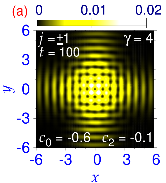
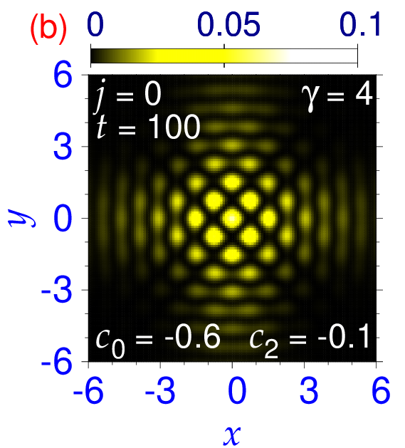
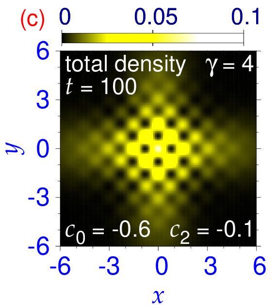
Figure 6: Contour plot of density of the super-lattice soliton, of Fig. 4(g)-(i), of components (a) $j=\pm 1,$ (b) $j=0$ and (c) total density, after real- time propagation at time $t=100$, using the converged imaginary-time wave function as the initial state.

The solitons considered here are dynamically stable. As an example, to demonstrate the dynamical stability, we consider the super-lattice soliton of Figs. 4(d)-(f) and subject the corresponding imaginary-time wave functions to real-time propagation during 100 units of time. The resultant real-time densities at time $t=100$ of the super-lattice soliton are displayed in Figs. 6 for components (a) $j=\pm 1$, (b) $j=0$ and (c) the total density. Although the root-mean-square sizes and energy were oscillating during real-time propagation, the periodic pattern in total density survived at $t=100$, which demonstrates the dynamical stability and ensures that these super-lattice solitons can be realized experimentally.

We demonstrated spontaneous spatial order in a Rashba SO-coupled uniform spin-1 quasi-2D ferromagnetic $(c_{2}<0)$ BEC for large SO-coupling strengths $\gamma$, and the formation of new types of dynamically stable super-lattice solitons using a numerical solution of the GP equation. The total density of these super-lattice solitons have a 2D square lattice formation. The component densities have either a stripe or a 2D square lattice density modulation. For small SO coupling, $(-1,0,+1)$ and $(0,+1,+2)$-type solitons are found, which develop multi-ring structure for intermediate SO coupling strengths. In addition, a circularly-asymmetric soliton is found to appear as the ground state for larger SO couplings. The dynamic stability of all these solitons was established by steady real-time propagation over a long period of time. Super-lattice solitons can also be formed in an SO-coupled anti-ferromagnetic $(c_{2}>0)$ BEC [33], the details of which are different from the present solitons. In the anti-ferromagnetic phase, the circularly-asymmetric and the $(0,\pm 1,\pm 2)$-type solitons are not possible, so that solitons of type displayed in Figs. 2(d)-(f), 3(a)-(c) and (g)-(i), and 4(a)-(c) will not appear. These dynamically-stable solitons deserve further experimental and theoretical studies. A natural extension of this investigation will be a search for a three-dimensional super-lattice soliton in an SO-coupled spin-1 BEC.

References

- [1] A. F. Andreev, I. M. Lifshitz, Zurn. Eksp. Teor. Fiz. 56 (1969) 2057 [English Transla.: Sov. Phys. JETP 29 (1969) 1107]; E. P. Gross, Phys. Rev. 106 (1957) 161; A. J. Leggett, Phys. Rev. Lett. 25 (1970) 1543; G. V. Chester, Phys. Rev. A 2 (1970) 256; V. I. Yukalov, Phys. 2 (2020) 49.
- [2] M. H. Anderson, J. R. Ensher, M. R. Matthews, C. E. Wieman, and E. A. Cornel, Science 269 (1995) 198; K. B. Davis, M.-O. Mewes, M. R. Andrews, N. J. van Druten, D. S. Durfee, D. M. Kurn, and W. Ketterle, Phys. Rev. Lett. 75 (1995) 3969.
- [3] M. W. Zwierlein, C. H. Schunck, A. Schirotzek, and W. Ketterle, Nature 442 (2006) 54; M. Greiner, C. A. Regal, and D. S. Jin, Nature 426 (2003) 537.
- [4] E. Kim and M. H. W. Chan, Nature 427 (2004) 225.
- [5] S. Balibar, Nature 464 (2010) 176.
- [6] K. Góral, L. Santos, M. Lewenstein, Phys. Rev. Lett. 88 (2002) 170406; L. Pollet, J. D. Picon, H. P. Büchler, and M. Troyer, Phys. Rev. Lett. 104 (2010) 125302; B. Capogrosso-Sansone, C. Trefzger, M. Lewenstein, P. Zoller, G. Pupillo, Phys. Rev. Lett. 104 (2010) 125301; S. Wessel and M. Troyer, Phys. Rev. Lett. 95 (2005) 127205.
- [7] R. Bombin, J. Boronat, F. Mazzanti, Phys. Rev. Lett. 119 (2017) 250402; Zhen-Kai Lu, Yun Li, D. S. Petrov, G. V. Shlyapnikov, Phys. Rev. Lett. 115 (2015) 075303; N. Y. Yao, C. R. Laumann, A. V. Gorshkov, S. D. Bennett, E. Demler, P. Zoller, M. D. Lukin Phys. Rev. Lett. 109 (2012) 266804.
- [8] G. Masella, A. Angelone, F. Mezzacapo, G. Pupillo, and N. V. Prokof’ev, Phys. Rev. Lett. 123 (2019) 045301; F. Cinti, P. Jain, M. Boninsegni, A. Micheli, P. Zoller, and G. Pupillo, Phys. Rev. Lett. 105 (2010) 135301; S. Saccani, S. Moroni, and M. Boninsegni, Phys. Rev. Lett. 108 (2012) 175301.
- [9] F. Böttcher, J.-N. Schmidt, M. Wenzel, J. Hertkorn, M. Guo, T. Langen, T. Pfau, Phys. Rev. X 9 (2019) 011051; J. Hertkorn, F. Böttcher, M. Guo, J. N. Schmidt, T. Langen, H. P. Büchler, T. Pfau, Phys. Rev. Lett. 123 (2019) 193002.
- [10] L. Tanzi, E. Lucioni, F. Famà, J. Catani, A. Fioretti, C. Gabbanini, R. N. Bisset, L. Santos, G. Modugno, Phys. Rev. Lett. 122 (2019) 130405; G. Natale, R. M. W. van Bijnen, A. Patscheider, D. Pet- ter, M. J. Mark, L. Chomaz, F. Ferlaino, Phys. Rev. Lett. 123 (2019) 050402.
- [11] T.-L. Ho, S. Zhang, Phys. Rev. Lett. 107 (2011) 150403.
- [12] Y. Li, G. I. Martone, L. P. Pitaevskii, S. Stringari, Phys. Rev. Lett. 110 (2013) 235302.
- [13] J. Dalibard, F. Gerbier, G. Juzeliunas, P. Öhberg, Rev. Mod. Phys. 83 (2011) 1523.
- [14] E. I. Rashba, Fiz. Tverd. Tela 2 (1960) 1224 [English Transla.: Sov. Phys. Solid State 2 (1960) 1109.]
- [15] G. Dresselhaus, Phys. Rev. 100 (1955) 580.
- [16] Y.-J. Lin, K. Jim énez-García, I. B. Spielman, Nature 471 (2011) 83.
- [17] J. Li, W. Huang, B. Shteynas, S. Burchesky, F. C. Top, E. Su, J. Lee, A. O. Jamison, W. Ketterle, Phys. Rev. Lett. 117 (2016) 185301.
- [18] D. Campbell, R. Price, A. Putra, A. Valdés-Curiel, D. Trypogeorgos, I. B. Spielman, Nat. Commun. 7 (2016) 10897.
- [19] J. Stenger, S. Inouye, D. M. Stamper-Kurn, H.-J. Mies- ner, A. P. Chikkatur, W. Ketterle, Nature 396 (1998) 345.
- [20] V. I. Yukalov, Laser Phys. 28 (2018) 053001; S. Gautam, S. K. Adhikari, Phys. Rev. A 92 (2015) 023616; Y. Kawaguchi, M. Ueda, Phys. Rep. 520 (2012) 253.
- [21] S. Sinha, R. Nath, and L. Santos, Phys. Rev. Lett. 107 (2011) 270401.
- [22] J.-R. Li, J. Lee, W. Huang, S. Burchesky, B. Shteynas, F. Ç. Top, A. O. Jamison, W. Ketterle, Nature 543 (2017) 91.
- [23] T. Mizushima, K. Machida, T. Kita, Phys. Rev. Lett. 89 (2002) (2002) 030401; T. Mizushima, K. Machida, T. Kita, Phys. Rev. A 66 (2002) 053610.
- [24] A. Putra, F. Salces-Carcoba, Y. Yue, S. Sugawa, I. B. Spielman, Phys. Rev. Lett. 124 (2020) 053605.
- [25] J. Léonard, A. Morales, P. Zupancic, T. Esslinger, T. Donner, Nature (London) 543, 87 (2017).
- [26] V. Achilleos, D. J. Frantzeskakis, P. G. Kevrekidis, D. E. Pelinovsky, Phys. Rev. Lett. 110 (2013) 264101.
- [27] H. Sakaguchi, B. Li, B. A. Malomed, Phys. Rev. E 89 (2014) 032920; H. Sakaguchi, B. A. Malomed, Phys. Rev. E 90 (2014) 062922.
- [28] Y.-C. Zhang, Z.-W. Zhou, B. A. Malomed, H. Pu, Phys. Rev. Lett. 115 (2015) 253902.
- [29] L. Salasnich, A. Parola, L. Reatto, Phys. Rev. A 65 (2002) 043614.
- [30] R. Ravisankar, D. Vudragović, P. Muruganandam, A. Balaž, S. K. Adhikari, Comput. Phys. Commun. 259 (2021) 107657; P. Muruganandam, S. K. Adhikari, Comput. Phys. Commun. 180 (2009) 1888; D. Vudragović, I. Vidanović, A. Balaž, P. Muruganandam, S. K. Adhikari, Comput. Phys. Commun. 183 (2012) 2021.
- [31] Y. V. Kartashov, D. A. Zezyulin, Phys. Rev. Lett. 122 (2019) 123201.
- [32] S. Gautam, S. K. Adhikari, Phys. Rev. A 91 (2015) 063617. S. Gautam, S. K. Adhikari, Laser Phys. Lett. 12 (2015) 045501.
- [33] S. K. Adhikari, unpublished.