Deep learning classification of bacteria clones explained by persistence homology

Abstract

In this work, we automatically distinguish between different clones of the same bacteria species (Klebsiella pneumoniae) based only on microscopic images. It is a challenging task, previously seemed unreachable due to the high clones’ similarity. For this purpose, we apply a multi-step algorithm with attention-based deep multiple instance learning, which returns parts of the image crucial to the prediction. Except for obtaining high accuracy, we introduce extensive explainability based on persistence homology, increasing the understandability and trust in the model. Our work opens a plethora of research pathways towards cheaper and faster epidemiological management.

I Introduction

Distinguishing between bacteria clones is a crucial part of the epidemiological management because it helps to discover source of the infection in a hospital and to prevent new cases. There exist several techniques to differentiate between bacteria clones, such as ribotyping [1], amplified fragment length polymorphism [2], multilocus sequence typing [3], and the most widely used pulsed-field gel electrophoresis [4, 5, 6]. However, all of them require costly equipment and reagents, and are highly unstable. Therefore, they must be repeated multiple times to obtain reliable results.

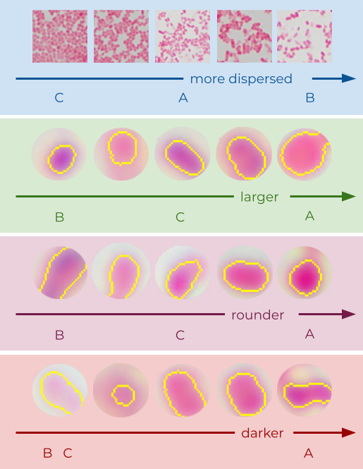
Figure 1: Summary of statistically significant differences between the clones $A$, $B$, and $C$ of Klebsiella pneumoniae based on the results presented in Section VII. Subsequent rows show differences in dispersion (blue arrows), size (green arrows), shape (purple arrows), and color (red arrows). Clone $A$ can be characterized as the largest, roundest, and darkest one - our method allows for description of distinct clones and finds features not visible to naked eye.

In this work, we automatically distinguish between different clones of the same bacteria species based only on microscopic images. This is an especially challenging task due to the high similarity of clones, as presented in Fig. 2, however, desirable due to acceleration of the diagnosis and reduction of the cost. To the best of our knowledge, it is the first attempt to solve this problem. Previous works either tried to use microscopic images to recognize bacteria morphology or classify different bacteria species [7], which is a much simpler task. As there exist no benchmarks we could use, we prepared an internal database containing $3$ clones with $31$ isolates of Klebsiella pneumoniae (see Fig. 2), a Gram-negative rod-shaped bacteria that may cause pneumonia, urinary tract infections or even sepsis [8, 9, 10].

Due to the large resolution of microscopic images, which cannot be scaled down due to loss of information, we first divide an image into patches, then generate their representations, and finally apply attention-based multiple instance learning, AbMILP [11], to classify clones. AbMILP aggregates representations using the attention mechanism that promotes essential patches. Therefore, except for the classification results, it also returns the attention scores that correspond to the patches’ importance. We also present results obtained using other techniques, like majority voting or mean and max pooling, but they either provide worse results or cannot be effectively explained. At the same time, in AbMILP, patches with the highest scores can be used to explain results obtained for a specific image, but they do not provide systematic characteristics of the clones, neither from the spatial arrangement nor from the individual cell perspective. This characteristic, however, is necessary to trust the model because microbiologists commonly assume that differentiating the clones of the same bacteria type based only on microscopic images seems unreachable.

To effectively explain the AbMILP, we introduce two methods based on essential patches segmented using CellProfiler [12]. The first one, based on persistence homology [13], analyzes the spatial arrangement of the bacteria, while the second one examines the size, shape, and color of the individual cells, as presented in Fig. 1. According to microbiologists, both XAI methods deliver a convincing explanation of the obtained results and increase the trust in the model.

The main contributions of this paper are as follows:

• Applying deep multiple instance learning to differentiate between bacteria clones based only on microscopic images (task previously seemed unreachable) with high accuracy.

• Introducing a new post-hoc explainability method based on persistence homology that measures differences in the spatial arrangement of cells between bacteria clones.

• Providing systematic characteristic of the clones (their size, shape, and color) from the individual cell perspective.

II Related works

Automatic pathogen classification based on microscopic images

Pathogen classification is a research problem addressed within different pathogens subgroups like bacteria [14, 15, 7], fungi [16, 17, 18], and protozoa [19, 20, 21]. In the case of bacteria, this topic was first examined in 1998 in  [14] where multi-layer perceptron was used to classify tuberculosis bacteria. Then, many approaches used hand-crafted features like perimeters, shapes, colors, contrast, and other morphological characteristics to distinguish between different bacteria species [22, 23, 24, 15]. There were, as well, deep learning based approaches [25, 26, 7, 27, 28, 29]. Most of the work was focused on detecting only a specific species of the bacteria, e.g. tuberculosis bacteria [14, 30, 31, 32, 33, 34, 35, 36, 37, 38]. Moreover, there was a lot of research in classifying the bacteria colonies. In [39] authors used SVM, in [40] one-class version of SVM with RBF kernel was used, and in [26] 2-layer CNN was employed. In summary, there was no research focused specifically on clone classification using microscopic images. And, even though there was some work on pathogen classification, none of methods used explainable AI to describe the rationale behind the prediction.

Post-hoc explainability in cells

There are only a few works touching on explainability of models for a cell classification. Among them is the research on the classification of the lung cancer [41] where CNN network was used to create a patch image representation and images were classified using bidirectional LSTM. The analysis of the LSTM gates showed that they are activated only when the patch contains cancer cells. Similar model was used in [42] but the explanations are based on the concept activation vectors [43] adapted to the regression problem. The next example of XAI applications in histology is colorectal cancer researched in [44] where cumulative fuzzy class membership criterion was used to explain the model decisions. Furthermore, [45] used self-attention and attention pooling maps to show the decisive parts of histology and fungi images, and [46] used class activation maps to show the key features on the images that decided the classification of the Clostridioides difficile bacteria cytotoxicity.

None of the previous works tried to utilize persistence homology to research dispersion characteristic of bacteria images. Moreover, according to best of our knowledge, there was no attempt to use Multiple Instance Learning to to characterize biomedical images on the level of singular cells.

III Material

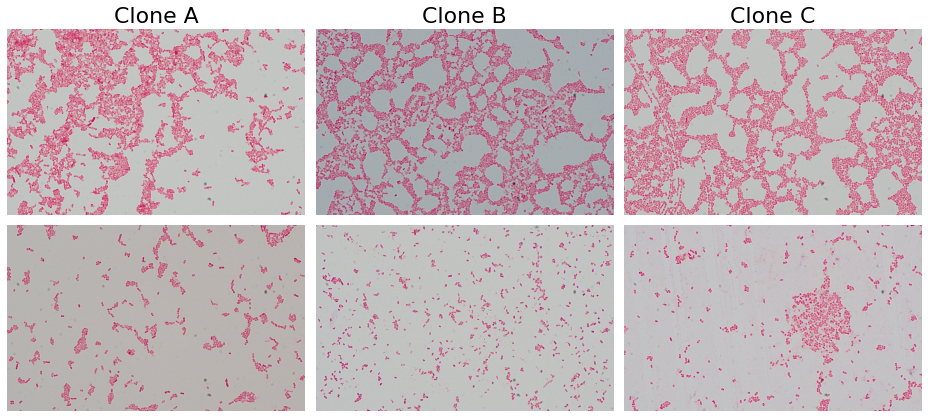
Figure 2: Sample images from our database visualize that different clones of Klebsiella pneumoniae are highly similar both from the spatial arrangement and from the individual cell perspective.

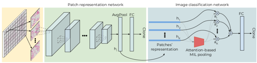
Figure 3: The pipeline of the method contains four steps. First, the image is divided into patches that are preprocessed and passed through the representation network. Then, the patches’ representations are aggregated with AbMILP to obtain one fixed-sized vector for each image. Finally, the vector is passed to the fully-connected layers of the network to classify the bacteria’s clone. Representation and classification networks are trained separately due to the large number of patches per image. As a result of applying AbMILP, it is possible to obtain systematic characteristics of the clones.

Our dataset contains $3$ clones of Klebsiella pneumoniae further described as clones $A$, $B$, and $C$, containing $11$, $10$, and $10$ isolates, respectively. Each isolate is represented by a set of $20$ images from $2$ preparations ($10$ images per preparation) to minimize the environmental bias. Isolates were obtained from patients of one hospital and come from the respiratory tract, urine, wound swabs, blood, fecal samples, catheter JJ, and urethral swab. All of the samples were Gram-stained and analyzed using an Olympus XC31 Upright Biological Microscope equipped with an Olympus SC30 camera to present Gram-negative organisms. They were photographed using Olympus D72 with $12$ bit image depth and saved as TIFF images of size $3500\times 5760$ pixels. Sample images from our database are presented in Fig. 2.

To cluster considered isolates into the clones, they were analyzed using pulsed-field gel electrophoresis (PFGE), a gold standard that relies on separating the DNA fragments after restriction cutting. PFGE profiles of the isolates were then interpreted using GelCompar software to obtain a dendrogram calculated with the Dice (band-based similarity) coefficient which is commonly used by microbiologists [47]. According to the dendrogram (partially presented in supplementary materials) isolates cluster into three clones. Clones $A$ and $B$ are similar (Dice score of $92\%$), while clone $C$ is more different from the others (Dice score of $77\%$). We use clones returned by GelCompar as the ground truth.

IV Method

We present the multi-step pipeline of our method in Fig. 3. Firstly, the image is divided into patches (defined below). Then, the foreground patches are preprocessed and passed through the patches representation network. Obtained representations are then aggregated using attention-based multiple instance learning [11] to obtain one fixed-sized vector for each image. Finally, such a vector can be passed to the successive fully-connected (FC) layers of the network to classify the bacteria’s clone. Due to the large number of patches per image, it is impossible to train the model at once. Therefore, we divided it into separately trained representation and classification networks using binary cross-entropy loss in both cases. They are described below, together with the preprocessing step.

Generating patches and preprocessing

Each image is scaled by a factor of $0.5$ and divided into the patches of resolution $250\times 250$ pixels using sliding window with stride $125$ (the optimal scale, resolution, and stride were obtained from preliminary experiments). To eliminate patches that are either empty or too populated with overlapping bacteria, we calculate standard deviation of the intensity of each patch, and reject patches with values lesser than $1.5$ (empty patches) and greater than $30$ (populous patches). The standard deviation thresholds were obtained experimentally. The remaining patches (most likely with non-overlapping bacteria) are normalized using the mean and the standard deviation computed based on $10000$ random training patches.

Patch representation network

Normalized patches are passed through ResNet-18 network [48] pretrained on ImageNet and then finetuned with the last layer containing three neurons corresponding to three considered clones (according to the preliminary experiment, a version without finetuning resulted in poor accuracy). The representations of the patches are obtained by taking the output of the penultimate layer.

Image classification network

To aggregate patches’ representations of an image, we apply attention-based multiple instance learning, AbMILP [11, 45]. It is a type of a weighted average pooling, in which the neural network determines weights of representations. More formally, if $\mathbf{h}=\{\mathbf{h_{i}}\in\mathbb{R}^{L}\}_{i=1}^{N}$ is the set of patches’ representations of an image, then the output of the operator is defined as:

$$\mathbf{z}=\sum_{i=1}^{N}a_{i}\mathbf{h_{i}},\textup{ where }a_{i}=\frac{\exp\left(\mathbf{w}^{T}tanh(\mathbf{Vh_{i}})\right)}{\sum_{j}^{N}\exp\left(\mathbf{w}^{T}tanh(\mathbf{Vh_{j}})\right)},$$ (1)

with $\mathbf{w}\in\mathbb{R}^{M}$ and $\mathbf{V}\in\mathbb{R}^{M\times L}$ being trainable layers of the neural network. Aggregated vector $\mathbf{z}$ is further processed by a dense layer with three output neurons corresponding to three considered clones.

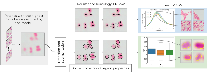
Figure 4: After training the model, we obtain patches that have the highest importance assigned by that model. We perform detection of cells on the patch and their segmentation. Then, pipeline divides into two paths. In the first one, we find centers of cells, we generate point cloud that is analyzed using persistence homology, and finally we obtain information about dispersion of cells in each clone. The second path consists of the border correction and finding region properties of the cells, resulting in information about the mean size, shape, and color of cells in each clone.

V Explainability

To explain which properties of bacteria are important for the AbMILP when distinguishing between two clones, we create a set of important patches that contains two patches with the highest attention weight ($a_{i}$ value) from each correctly predicted image. We decided to analyze such a set because it includes patches with the greatest influence on the results.

In Fig. 4, we present two types of the analysis conducted on such essential patches. The first one, based on persistence homology [13], analyzes the spatial arrangement of the bacteria, while the second one examines the size, shape, and color of the individual cells. Both types of the analysis are preceded by bacteria cells’ segmentation obtained using CellProfiler [12] with a pipeline describe below.

Segmentation of bacteria

To segment bacteria, we first transform a patch into the grayscale images and then apply a CellProfiler pipeline with only one component identifying primary objects with a typical diameter between $10$ and $40$ pixels. The objects with diameters outside this range are discarded along with objects touching the border. The result of segmentation for sample patches is presented in supplementary materials.

Spatial arrangement of bacteria

For each segmentation of a patch, we generate a point cloud $C\subset\mathbb{R}^{2}$ containing centers of the segmented bacteria and analyze this point cloud using persistence homology [13], that provides a comprehensive, multiscale summary of the underlying data’s shape and is currently gaining increasing importance in data science [49].

Persistence homology can be defined for a continuous function $f:C\rightarrow\mathbb{R}$, typically a distance function from a collection of points (in this case, centers of the bacteria). Focusing on sub-level sets $L_{c}=f^{-1}((-\infty,c])$, we let $c$ grow from $-\infty$ to $+\infty$. While this happens, we can observe a hierarchy of events. In dimension $0$, connected components of $L_{c}$ are created and merged. In dimension $1$, cycles that are not bounded or higher dimensional voids appear in $L_{c}$ at critical points of $f$. The value of $c$ on which a connected component, cycle or a higher dimensional void, appears is referred to as birth time. They subsequently either become identical (up to a deformation) to other cycles and voids (created earlier) or glued-in and become trivial. The value of $c$ on which that happens is referred to as death time. As a result, every connected component, a cycle, or a higher dimensional void can be characterized by a pair of numbers, $b$ and $d$, the birth and death time. Therefore, a set of birth-death pairs is obtained, called a persistence diagram or a persistence barcode. They are not easy to compare due to their variable size. Therefore, we apply a vectorization method called persistence bag of words [50, 51] to obtain a fixed-size representation for each patch. Based on them, we calculate the average persistence bag of words for each clone and analyze differences in representative patches. for more information about persistent homology please see [52].

Properties of individual bacteria

To understand what differentiates individual cells between the clones, we limit segments obtained from CellProfiler to those isolated from the others (with no adjacent segments). As the boundaries of cells returned by CellProfiler are not ideal, we correct them using Otsu thresholding on a dilated segment. Then, we fit an ellipse to the corrected segment and analyze significant differences between clones, such as distributions of size, shape (minor to major axis length), and color. See supplementary materials for details.

VI Experiment setup

We train the representation network and classification network $5$ time using cross-validation to obtain reliable results for each configuration. To create a training and test set for each fold, we randomly choose one of two isolate’s preparations and add it to the training set. The remaining preparation is added to the test set.

TABLE I: Results of Image-based Classification for Seven Tested Methods With the Best Scores in Bold Based on Wilcoxon Signed-rank Test.

Method	Accuracy	Precision	Recall	F1	AUC
instance + mv	$\mathbf{63.8\pm 1.1}$	$64.1\pm 1.0$	$\mathbf{63.8\pm 1.1}$	$\mathbf{63.8\pm 1.0}$	$n/a$
instance + max	$59.3\pm 3.6$	$59.8\pm 3.5$	$59.3\pm 3.6$	$59.3\pm 3.6$	$75.0\pm 2.5$
instance + mean	$59.7\pm 2.7$	$60.5\pm 2.7$	$59.7\pm 2.7$	$59.8\pm 2.7$	$\mathbf{78.6\pm 2.5}$
embedding + max	$56.3\pm 6.9$	$52.9\pm 11.0$	$56.3\pm 6.9$	$52.9\pm 9.9$	$68.3\pm 9.6$
embedding + mean	$58.4\pm 5.9$	$58.9\pm 6.3$	$58.4\pm 5.9$	$\mathbf{58.0\pm 6.2}$	$73.4\pm 5.1$
embedding + AbMILP	$\mathbf{64.8\pm 2.2}$	$\mathbf{66.9\pm 1.4}$	$\mathbf{64.8\pm 2.2}$	$\mathbf{64.3\pm 2.4}$	$\mathbf{77.3\pm 2.7}$
embedding + SA-AbMILP	$62.7\pm 2.0$	$63.5\pm 1.8$	$62.7\pm 2.0$	$62.3\pm 2.2$	$\mathbf{78.1\pm 1.9}$

The representation network is finetuned with batch size $64$ and initial learning rate $0.0001$, decreasing $10$ times after every $1000$ steps. Hyperparameters were obtained during preliminary experiments which included different constant learning rates in range [$0.00000001,0.001$] and batch size values: $16,32,64$. In these experiment we used only the training set. All network layers are finetuned with binary cross-entropy loss and weighted sampling to reduce the influence of data imbalance and were trained for $5000$ iterations, up to a point of flattening of the loss function. Training images were augmented using color jittering, random rotation, and random flip.

To obtain the best hyperparameters for the classification network we applied grid search over learning rate in the range [$0.000005$, $0.001$] and weight decay in the range [$0.00001$, $0.05$]. We use a standard number of attention heads ($3$) as according to [11] this parameter is not relevant.

When it comes to explainability, we build the Vietoris-Rips complex from the distance matrix, based on which we then calculate persistence homology of dimension $0$ using the Gudhi library [53]. As a result, we obtain persistence diagrams with birth time equal to $0$ in all its points. Based on them, we generate a persistence bag of words with $128$ regular codewords of size $1$ with cluster centers in $0.5,1.5,2.5,\dots,127.5$ of death time.

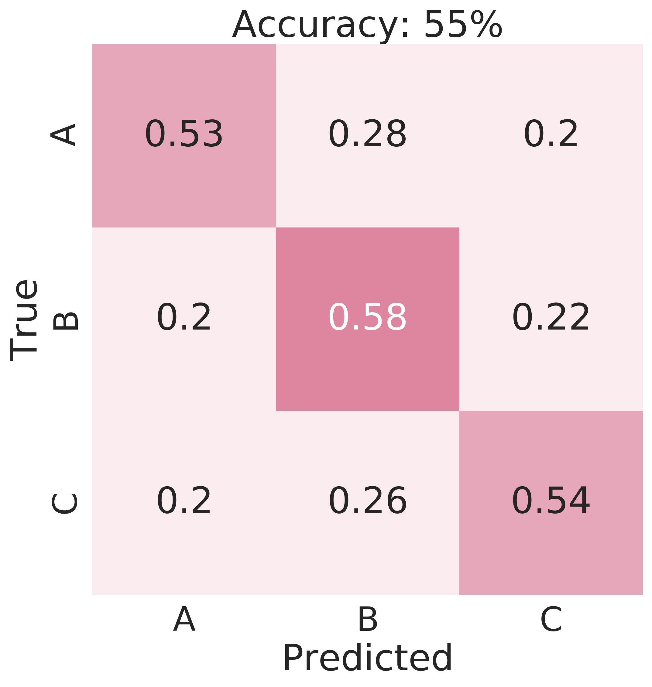
(a) CNN

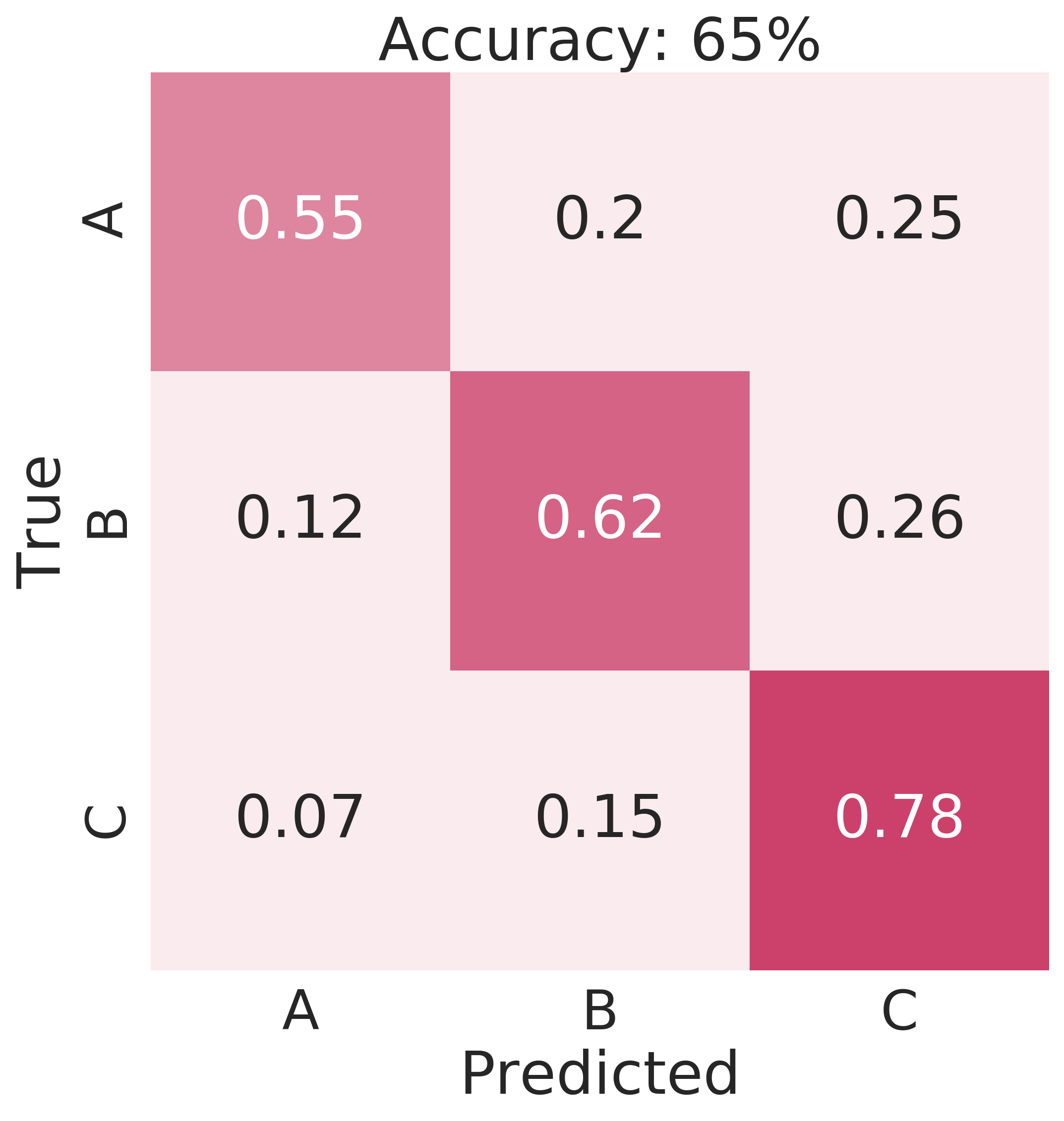
(b) AbMILP

Figure 5: Confusion matrices for representation (CNN) and classification (AbMILP) networks averaged over $5$ folds and calculated on test subset. Usage of attention-based pooling visibly improves accuracy.

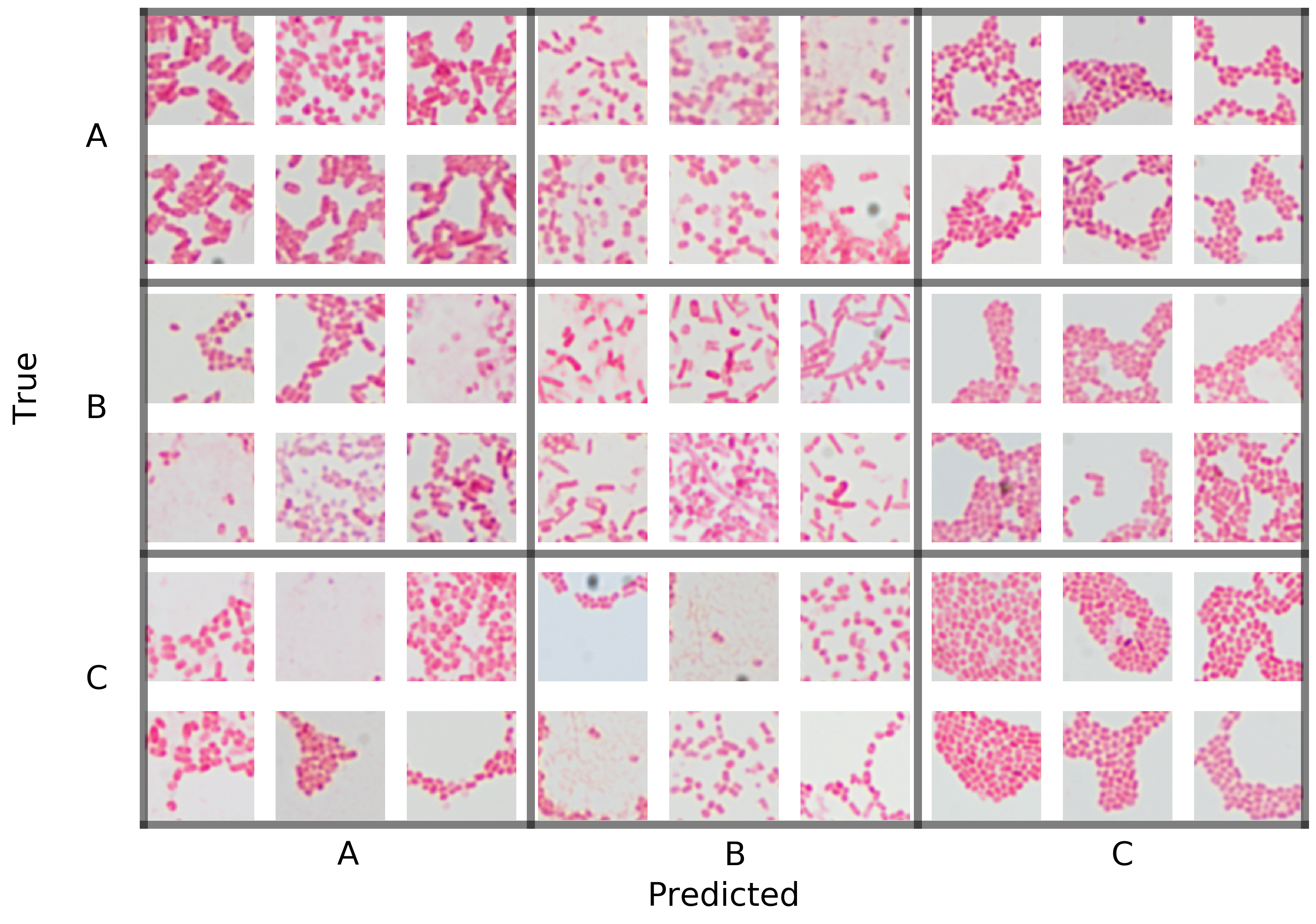
(a) CNN

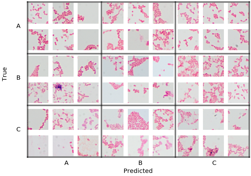
(b) AbMILP

Figure 6: Qualitative confusion matrices for representation (CNN) and classification (AbMILP) networks, for fold $0$ of test subset. Each confusion matrix cell contains $6$ ($2\times 3$) representative patches coming from different images. We cannot notice any unique characteristic of clones based on the patches from AbMILP. Thus, we introduce methods described in Sec. V to find those characteristics.

We test variety of pooling methods to perform per image classification, because per patch results given by using only the CNN were not satisfactory with $54.9\%\pm 2.2\%$ accuracy. Methods used to obtain per image results:

• instance + mv: majority voting performed on all the patches in the image.

• instance + max: max pooling performed on representation network output.

• instance + mean: mean pooling performed on representation network output.

• embedding + max: max pooling performed on embeddings obtained from penultimate layer of representation network.

• embedding + mean: mean pooling performed on embeddings obtained from penultimate layer of representation network.

• embedding + AbMILP: attention based pooling performed on embeddings obtained from penultimate layer of representation network.

• embedding + SA-AbMILP: attention based pooling with self-attention kernel [45] performed on embeddings obtained from penultimate layer of representation network.

We perform all the experiments on a workstation with two $23$ GB GPU and $128$ GB RAM. On average, it takes $30$ hours to train a patch representation network and $8$ hours to generate patch representations for the classification step. Training of image classification network lasts up to $1$ hour. Both networks were implemented using PyTorch. The code is publicly available.

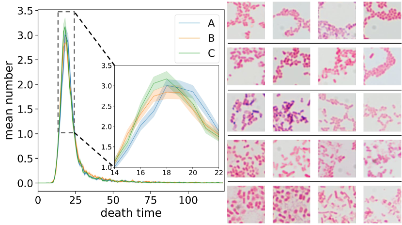
Figure 7: The average persistence bag of words for clone C is significantly higher than clone B in the $[14;22]$ death time interval. It means that many clone C bacteria are localized close to each other (the upper row of patches) and merge faster than clone B bacteria that are more dispersed (the bottom row of patches). It is one of the many conclusions drawn by the explainability framework based on the persistence homology.

VII Results

VII-A Classification

Results are presented in Fig. 5 in the form of confusion matrices averaged over five folds for patch representation and image classification networks. They clearly indicate that it is possible to differentiate between bacteria clones based only on microscopic images with high accuracy. Moreover, while patch-based test accuracy can be relatively low at $55\%$, it can be compensated by attention-based pooling which obtains the accuracy of image-based classification at the level of $65\%$, whilst the accuracy of a random classifier is $33\%$. Confusion matrix of the image-based model indicates higher accuracy when classifying clone C. However, it is expected because it is more genetically distant to other clones and there are more similarities between clones $A$ and $B$.

In Tab. I, we present per-image results for the seven tested methods. The AbMILP method gives significantly better results, based on Wilcoxon signed-rank test, than other methods across all metrics and majority voting obtains almost as good results. However, in contrast to AbMILP and SA-AbMILP, majority voting is not useful method when trying to explain the model. Most probably, AbMILP achieves the best results because it is an approach fully parameterized by neural networks, which uses information from each of the instances in a weighted manner. It is surprising that AbMILP obtains better results than SA-AbMILP, nonetheless, we did not test all possible kernels in the later.

VII-B Explainability

As the first type of a model explanation, we present quantitative confusion matrices obtained for test set by representation and classification networks (see Fig. 6). While some trends are visible in representation networks, such as the more dispersed distribution of clone $B$, no systematic characteristic can be implicated in AbMILP, which demonstrates the need to explain it with more sophisticated explainability methods.

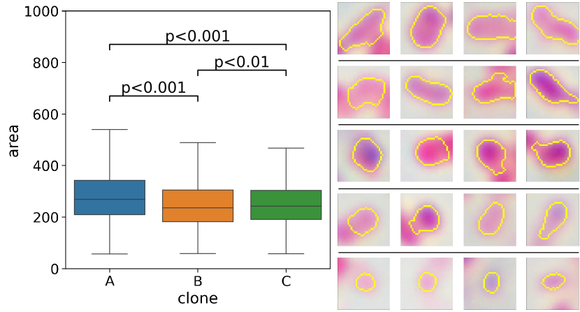
(a) distribution of size

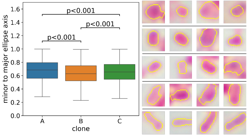
(b) distribution of shape (roundness)

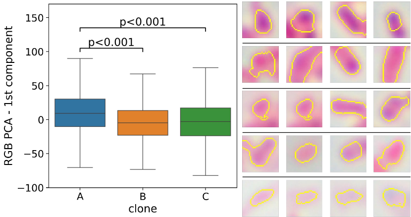
(c) distribution of color intensity

Figure 8: Distributions of size (a), shape (b), and color intensity (c), as well as sample bacteria cells from the lowest (left side) to the highest value (right side) of considered properties. In all cases differences between distributions are statistically significant and the only exception is the distribution of color intensity between clones $B$ and $C$.

The first method is based on the persistence bag of words (PBoW) generated for the point clouds obtained for all important patches. In Fig. 7, we present the average PBoW for all three clones that can be used to draw many interesting conclusions. Firstly, the average PBoW differs mostly between 14 and 22 death time and is the highest for clone C. This means that clone C contains much more cells merging at the initial stage of filtration. Hence, its cells are much closer to each other than in the case of clones A and B. Moreover, while clone B and C are in line in the interval [14; 22], although B is generally lower than C, the average PBoW for clone A is moved toward the right side of the plot. This means that clone B has either very close or very distant cells, while clone A contains rather slightly more distant cells than in the case of clone C.

In Fig. 8 we present more individual properties of the bacteria, such as the larger size of bacterial cells from clones $A$ and $C$ comparing to clone $B$. One can also observe that bacterial cells of clone $A$ are larger and darker than in clones $B$ and $C$. Moreover, bacterial cells of clone $A$ are also significantly rounder than in clone $B$. Simultaneously, bacterial cells of clone $A$ are darker than in clones $B$ and $C$. We hypothesize that it can be caused by the presence of a polysaccharide capsule (envelope). More precisely, the thicker capsule results in darker color caused by dye retention during staining, rounder shape caused by the limited ability to reshape, and larger size due to dye accumulation both in the cell and in the envelope. We present a summary of the clones’ properties in Fig. 1.

VIII Conclusion

In this work, we analyzed if it is possible to distinguish between different clones of the same bacteria species (Klebsiella pneumoniae) based only on microscopic images. To address this challenging task, which previously seemed unreachable, we applied a multi-step algorithm with attention-based multiple instance learning (AbMILP), which resulted in an accuracy of $65\%$. Moreover, we pointed out the AbMILP interpretation’s weaknesses, and we introduced more efficient explainability methods based on CellProfiler segmentation and persistence homology.

The extensive analysis revealed systematic differences between the clones from the spatial arrangement and the individual cell perspective. Hence, in the future, we plan to use this knowledge and cluster the isolates into clones using unsupervised methods to obtain cheaper and faster epidemiological management.

References

- [1] S. Bratu, D. Landman, R. Haag, R. Recco, A. Eramo, M. Alam, and J. Quale, “Rapid spread of carbapenem-resistant klebsiella pneumoniae in new york city,” Archives of Internal Medicine, vol. 165, no. 12, p. 1430, Jun. 2005. [Online]. Available: https://doi.org/10.1001/archinte.165.12.1430
- [2] D. Jonas, B. Spitzmüller, F. D. Daschner, J. Verhoef, and S. Brisse, “Discrimination of klebsiella pneumoniae and klebsiella oxytoca phylogenetic groups and other klebsiella species by use of amplified fragment length polymorphism,” Research in Microbiology, vol. 155, no. 1, pp. 17–23, Jan. 2004. [Online]. Available: https://doi.org/10.1016/j.resmic.2003.09.011
- [3] L. Diancourt, V. Passet, J. Verhoef, P. A. D. Grimont, and S. Brisse, “Multilocus sequence typing of klebsiella pneumoniae nosocomial isolates,” Journal of Clinical Microbiology, vol. 43, no. 8, pp. 4178–4182, Aug. 2005. [Online]. Available: https://doi.org/10.1128/jcm.43.8.4178-4182.2005
- [4] H. Han, H. Zhou, H. Li, Y. Gao, Z. Lu, K. Hu, and B. Xu, “Optimization of pulse-field gel electrophoresis for subtyping of klebsiella pneumoniae,” International Journal of Environmental Research and Public Health, vol. 10, no. 7, pp. 2720–2731, Jul. 2013. [Online]. Available: https://doi.org/10.3390/ijerph10072720
- [5] Y. J. Lau, B. S. Hu, W. L. Wu, Y. H. Lin, H. Y. Chang, and Z. Y. Shi, “Identification of a major cluster of Klebsiella pneumoniae isolates from patients with liver abscess in Taiwan,” J. Clin. Microbiol., vol. 38, no. 1, pp. 412–414, 1 2000.
- [6] K. Mamlouk, I. B.-B. Boubaker, V. Gautier, S. Vimont, B. Picard, S. B. Redjeb, and G. Arlet, “Emergence and outbreaks of CTX-m -lactamase-producing escherichia coli and klebsiella pneumoniae strains in a tunisian hospital,” Journal of Clinical Microbiology, vol. 44, no. 11, pp. 4049–4056, Sep. 2006. [Online]. Available: https://doi.org/10.1128/jcm.01076-06
- [7] B. Zieliński, A. Plichta, K. Misztal, P. Spurek, M. Brzychczy-Włoch, and D. Ochońska, “Deep learning approach to bacterial colony classification,” PloS one, vol. 12, no. 9, p. e0184554, 2017.
- [8] C.-P. Fung, F.-Y. Chang, S.-C. Lee, B.-S. Hu, B. I.-T. Kuo, C.-Y. Liu, M. Ho, and L. K. Siu, “A global emerging disease of klebsiella pneumoniae liver abscess: is serotype k1 an important factor for complicated endophthalmitis?” Gut, vol. 50, no. 3, pp. 420–424, 2002. [Online]. Available: https://gut.bmj.com/content/50/3/420
- [9] E. M. Karama, F. Willermain, X. Janssens, M. Claus, S. V. den Wijngaert, J.-T. Wang, C. Verougstraete, and L. Caspers, “Endogenous endophthalmitis complicating klebsiella pneumoniae liver abscess in europe: case report,” International Ophthalmology, vol. 28, no. 2, pp. 111–113, Aug. 2007. [Online]. Available: https://doi.org/10.1007/s10792-007-9111-4
- [10] W.-C. Ko, “Community-acquired klebsiella pneumoniae bacteremia: Global differences in clinical patterns,” Emerging Infectious Diseases, vol. 8, no. 2, pp. 160–166, Feb. 2002. [Online]. Available: https://doi.org/10.3201/eid0802.010025
- [11] M. Ilse, J. Tomczak, and M. Welling, “Attention-based deep multiple instance learning,” in Proceedings of the 35th International Conference on Machine Learning, ser. Proceedings of Machine Learning Research, J. Dy and A. Krause, Eds., vol. 80. Stockholmsmässan, Stockholm Sweden: PMLR, 10–15 Jul 2018, pp. 2127–2136. [Online]. Available: http://proceedings.mlr.press/v80/ilse18a.html
- [12] A. E. Carpenter, T. R. Jones, M. R. Lamprecht, C. Clarke, I. H. Kang, O. Friman, D. A. Guertin, J. H. Chang, R. A. Lindquist, J. Moffat et al., “Cellprofiler: image analysis software for identifying and quantifying cell phenotypes,” Genome biology, vol. 7, no. 10, p. R100, 2006.
- [13] H. Edelsbrunner, D. Letscher, and A. Zomorodian, “Topological persistence and simplification,” in Proceedings 41st annual symposium on foundations of computer science. IEEE, 2000, pp. 454–463.
- [14] K. Veropoulos, G. Learmonth, C. Campbell, B. Knight, and J. Simpson, “Automated identification of tubercle bacilli in sputum. a preliminary investigation.” Analytical and quantitative cytology and histology, vol. 21, no. 4, p. 277, 1999.
- [15] M. Chayadevi and G. Raju, “Extraction of bacterial clusters from digital microscopic images through statistical and neural network approaches,” in Proceedings of International Conference on Advances in Computing. Springer, 2013, pp. 1091–1099.
- [16] J. Zhang, S. Lu, X. Wang, X. Du, G. Ni, J. Liu, L. Liu, and Y. Liu, “Automatic identification of fungi in microscopic leucorrhea images,” JOSA A, vol. 34, no. 9, pp. 1484–1489, 2017.
- [17] M. W. Tahir, N. A. Zaidi, A. A. Rao, R. Blank, M. J. Vellekoop, and W. Lang, “A fungus spores dataset and a convolutional neural network based approach for fungus detection,” IEEE transactions on nanobioscience, vol. 17, no. 3, pp. 281–290, 2018.
- [18] B. Zieliński, A. Sroka-Oleksiak, D. Rymarczyk, A. Piekarczyk, and M. Brzychczy-Włoch, “Deep learning approach to description and classification of fungi microscopic images,” PloS one, 2020.
- [19] K. W. Widmer, K. H. Oshima, and S. D. Pillai, “Identification of cryptosporidium parvum oocysts by an artificial neural network approach,” Applied and environmental microbiology, vol. 68, no. 3, pp. 1115–1121, 2002.
- [20] C. A. Castañón, J. S. Fraga, S. Fernandez, A. Gruber, and L. d. F. Costa, “Biological shape characterization for automatic image recognition and diagnosis of protozoan parasites of the genus eimeria,” Pattern Recognition, vol. 40, no. 7, pp. 1899–1910, 2007.
- [21] S. Kosov, K. Shirahama, C. Li, and M. Grzegorzek, “Environmental microorganism classification using conditional random fields and deep convolutional neural networks,” Pattern Recognition, vol. 77, pp. 248–261, 2018.
- [22] J. Liu, F. B. Dazzo, O. Glagoleva, B. Yu, and A. K. Jain, “Cmeias: a computer-aided system for the image analysis of bacterial morphotypes in microbial communities,” Microbial Ecology, vol. 41, no. 3, pp. 173–194, 2001.
- [23] L. Xiaojuan and C. Cunshe, “An improved bp neural network for wastewater bacteria recognition based on microscopic image analysis,” WSEAS Transactions on computers, vol. 8, no. 2, pp. 237–247, 2009.
- [24] S. Kumar and G. S. Mittal, “Rapid detection of microorganisms using image processing parameters and neural network,” Food and Bioprocess Technology, vol. 3, no. 5, pp. 741–751, 2010.
- [25] D. Nie, E. A. Shank, and V. Jojic, “A deep framework for bacterial image segmentation and classification,” in Proceedings of the 6th ACM Conference on Bioinformatics, Computational Biology and Health Informatics, 2015, pp. 306–314.
- [26] G. Turra, S. Arrigoni, and A. Signoroni, “Cnn-based identification of hyperspectral bacterial signatures for digital microbiology,” in International Conference on Image Analysis and Processing. Springer, 2017, pp. 500–510.
- [27] M. F. Wahid, T. Ahmed, and M. A. Habib, “Classification of microscopic images of bacteria using deep convolutional neural network,” in 2018 10th International Conference on Electrical and Computer Engineering (ICECE). IEEE, 2018, pp. 217–220.
- [28] N. Rahmayuna, D. S. Rahardwika, C. A. Sari, E. H. Rachmawanto et al., “Pathogenic bacteria genus classification using support vector machine,” in 2018 International Seminar on Research of Information Technology and Intelligent Systems (ISRITI). IEEE, 2018, pp. 23–27.
- [29] T. Ahmed, M. F. Wahid, and M. J. Hasan, “Combining deep convolutional neural network with support vector machine to classify microscopic bacteria images,” in 2019 International Conference on Electrical, Computer and Communication Engineering (ECCE). IEEE, 2019, pp. 1–5.
- [30] M. K. Osman, F. Ahmad, Z. Saad, M. Y. Mashor, and H. Jaafar, “A genetic algorithm-neural network approach for mycobacterium tuberculosis detection in ziehl-neelsen stained tissue slide images,” in 2010 10th International Conference on Intelligent Systems Design and Applications. IEEE, 2010, pp. 1229–1234.
- [31] Y. Zhai, Y. Liu, D. Zhou, and S. Liu, “Automatic identification of mycobacterium tuberculosis from zn-stained sputum smear: Algorithm and system design,” in 2010 IEEE International Conference on Robotics and Biomimetics. IEEE, 2010, pp. 41–46.
- [32] R. Rulaningtyas, A. B. Suksmono, and T. L. Mengko, “Automatic classification of tuberculosis bacteria using neural network,” in Proceedings of the 2011 International Conference on Electrical Engineering and Informatics. IEEE, 2011, pp. 1–4.
- [33] L. Govindan, N. Padmasini, and M. Yacin, “Automated tuberculosis screening using zeihl neelson image,” in 2015 IEEE International Conference on Engineering and Technology (ICETECH). IEEE, 2015, pp. 1–4.
- [34] P. Ghosh, D. Bhattacharjee, and M. Nasipuri, “A hybrid approach to diagnosis of tuberculosis from sputum,” in 2016 International Conference on Electrical, Electronics, and Optimization Techniques (ICEEOT). IEEE, 2016, pp. 771–776.
- [35] E. Priya and S. Srinivasan, “Automated object and image level classification of tb images using support vector neural network classifier,” Biocybernetics and Biomedical Engineering, vol. 36, no. 4, pp. 670–678, 2016.
- [36] Y. P. López, C. F. Costa Filho, L. Aguilera, and M. Costa, “Automatic classification of light field smear microscopy patches using convolutional neural networks for identifying mycobacterium tuberculosis,” in 2017 CHILEAN Conference on Electrical, Electronics Engineering, Information and Communication Technologies (CHILECON). IEEE, 2017, pp. 1–5.
- [37] R. O. Panicker, K. S. Kalmady, J. Rajan, and M. Sabu, “Automatic detection of tuberculosis bacilli from microscopic sputum smear images using deep learning methods,” Biocybernetics and Biomedical Engineering, vol. 38, no. 3, pp. 691–699, 2018.
- [38] K. Mithra and W. S. Emmanuel, “Automated identification of mycobacterium bacillus from sputum images for tuberculosis diagnosis,” Signal, Image and Video Processing, vol. 13, no. 8, pp. 1585–1592, 2019.
- [39] H. Men, Y. Wu, Y. Gao, Z. Kou, Z. Xu, and S. Yang, “Application of support vector machine to heterotrophic bacteria colony recognition,” in 2008 International Conference on Computer Science and Software Engineering, vol. 1. IEEE, 2008, pp. 830–833.
- [40] W.-B. Chen and C. Zhang, “An automated bacterial colony counting and classification system,” Information Systems Frontiers, vol. 11, no. 4, pp. 349–368, 2009.
- [41] G. Campanella, M. G. Hanna, L. Geneslaw, A. Miraflor, V. W. K. Silva, K. J. Busam, E. Brogi, V. E. Reuter, D. S. Klimstra, and T. J. Fuchs, “Clinical-grade computational pathology using weakly supervised deep learning on whole slide images,” Nature medicine, vol. 25, no. 8, pp. 1301–1309, 2019.
- [42] M. Graziani, V. Andrearczyk, and H. Müller, “Regression concept vectors for bidirectional explanations in histopathology,” in Understanding and Interpreting Machine Learning in Medical Image Computing Applications. Springer, 2018, pp. 124–132.
- [43] B. Kim, M. Wattenberg, J. Gilmer, C. Cai, J. Wexler, F. Viegas et al., “Interpretability beyond feature attribution: Quantitative testing with concept activation vectors (tcav),” in International conference on machine learning. PMLR, 2018, pp. 2668–2677.
- [44] P. Sabol, P. Sinčák, P. Hartono, P. Kočan, Z. Benetinová, A. Blichárová, L. Verbóová, E. Štammová, A. Sabolová-Fabianová, and A. Jašková, “Explainable classifier for improving the accountability in decision-making for colorectal cancer diagnosis from histopathological images,” Journal of Biomedical Informatics, vol. 109, p. 103523, 2020.
- [45] D. Rymarczyk, A. Borowa, J. Tabor, and B. Zieliński, “Kernel self-attention for weakly-supervised image classification using deep multiple instance learning,” in Proceedings of the IEEE/CVF Winter Conference on Applications of Computer Vision, 2021, pp. 1721–1730.
- [46] A. Brodzicki, J. Jaworek-Korjakowska, P. Kleczek, M. Garland, and M. Bogyo, “Pre-trained deep convolutional neural network for clostridioides difficile bacteria cytotoxicity classification based on fluorescence images,” Sensors, vol. 20, no. 23, p. 6713, 2020.
- [47] A. Rementeria, L. Gallego, G. Quindós, and J. Garaizar, “Comparative evaluation of three commercial software packages for analysis of dna polymorphism patterns,” Clinical Microbiology and Infection, vol. 7, no. 6, pp. 331–336, 2001. [Online]. Available: https://www.sciencedirect.com/science/article/pii/S1198743X14624848
- [48] K. He, X. Zhang, S. Ren, and J. Sun, “Deep residual learning for image recognition,” CoRR, vol. abs/1512.03385, 2015. [Online]. Available: http://arxiv.org/abs/1512.03385
- [49] M. Ferri, “Persistent topology for natural data analysis—a survey,” in Towards Integrative Machine Learning and Knowledge Extraction. Springer, 2017, pp. 117–133.
- [50] B. Zieliński, M. Lipiński, M. Juda, M. Zeppelzauer, and P. Dłotko, “Persistence bag-of-words for topological data analysis,” in Proceedings of the 28th International Joint Conference on Artificial Intelligence. AAAI Press, 2019, pp. 4489–4495.
- [51] ——, “Persistence codebooks for topological data analysis,” Artificial Intelligence Review, pp. 1–41, 2020.
- [52] H. Edelsbrunner and J. Harer, Computational topology: an introduction. American Mathematical Soc., 2010.
- [53] C. Maria, J.-D. Boissonnat, M. Glisse, and M. Yvinec, “The gudhi library: Simplicial complexes and persistent homology,” in International Congress on Mathematical Software. Springer, 2014, pp. 167–174.