New Algorithms And Fast Implementations To Approximate Stochastic Processes

Abstract

We present new algorithms and fast implementations to find efficient approximations for modelling stochastic processes. For many numerical computations it is essential to develop finite approximations for stochastic processes. While the goal is always to find a finite model, which represents a given knowledge about the real data process as accurate as possible, the ways of estimating the discrete approximating model may be quite different: (i) if the stochastic model is known as a solution of a stochastic differential equation, e.g., one may generate the scenario tree directly from the specified model; (ii) if a simulation algorithm is available, which allows simulating trajectories from all conditional distributions, a scenario tree can be generated by stochastic approximation; (iii) if only some observed trajectories of the scenario process are available, the construction of the approximating process can be based on non-parametric conditional density estimates.

We also elaborate on the important concept of distances, which allows us to assess the quality of the approximation. We study these methods and apply them to an electricity price data.

Our fast implementation

ScenTrees.jl

including an exhaustive documentation is available for free at GitHub.

Keywords: Decision making under uncertainty, scenario tree generation, scenario lattice generation, nested distance

Classification: 90C15, 60B05, 62P05

1 Introduction

A decision maker can formulate an action plan to achieve a specific goal. The action plan is executed in sequential stages. Planning under uncertainty considers already at the beginning random events which might happen while the plan is executed, taking the possibility of corrective (recourse) decisions into account. This ensures that the desired goal can be met, even in an uncertain environment where random events impact and influence the situation at each stage.

An important historical contribution in the development of decision making under uncertainty is Markowitz (1952), who considers an optimal asset allocation problem and developed what is nowadays called modern portfolio theory. This example is often used to illustrate and outline the difficulty: an investment decision has to be made today, but the random return is observed after the investment horizon, in the future. In its simplest version, the problem has only one decision stage, but if a recourse decision is allowed after the random outcome is revealed, the problem is said to be two-stage. However, if financial securities such as options with different maturities are included in the portfolio then more decision stages must be considered: intermediate decisions have to be made whenever options expire before reaching the investment horizon; the problem is then said to be multistage.

Further problems dealing with decision making under uncertainty appear in logistics and inventory control. Goods must be shipped between various warehouses in view of random demands and unmatched demand triggers recourse actions by rapid new orders (cf. Dantzig (1955) for a very early problem description). This problem can be formulated as a decision problem in multiple stages. Optimal inventory and transportation policies constitute hedging strategies against unknown and varying demands.

As another problem with economic relevance we mention an optimal schedule to manage reservoirs of a hydropower plant. Its inflows are rain and perhaps melting snow, which are both random events. The price of electricity produced is highly volatile in addition, so that the optimal operation mode is a sequence of decisions, made at consecutive times and influenced by various random events (cf. Séguin et al. (2017) for a more concrete discussion).

All problems mentioned above have uncertain scenarios and decisions at intermediate stages in common. The scenarios appear as the trajectories of a stochastic process in discrete time, $\xi=(\xi_{1},\dots,\xi_{T})$, with values $\xi_{t}\in\mathbb{R}^{m_{t}}$, say. For algorithmic treatment, such general processes must be approximated by simpler ones, in the same manner as functions are represented as vectors on finite grids on digital computers. In particular, a discrete time stochastic process is approximated by a scenario tree or, in case of a Markovian process, by a scenario lattice. Notice, however, that quite often the decisions at earlier stages influence the feasibility of profitability of later stages and in such a case the full history of the decision process has to be recorded. The history process is always a tree.

An elementary component for generating scenario trees is the approximation of a random outcome, i.e., the approximation of random variables. An example is the random realization $\xi_{1}$ at the first stage, which has to be approximated sufficiently well for an algorithmic treatment. Graf and Luschgy (2000) provide a comprehensive study and theoretical background on this topic (called also uncertainty vector quantification), Pagès and Printems (2005) and Bally et al. (2005) present methods and algorithms, many of them are based on optimal clustering, cf. Hartigan (1975). It is an important observation that the approximation of a random outcome as $\xi_{1}$ suffers from the curse of dimensionality, a term coined by R. Bellman (cf. Bellman (1961); Dudley (1969)).

The generation of scenario trees is even more involved. Indeed, not only one random realization as $\xi_{1}$ has to be approximated, but the entire underlying stochastic process $(X_{1},\dots,X_{T})$, often with complicated interdependencies. Consequently, the approximation of the stochastic process is significantly more complex and computationally more expensive.

Høyland and Wallace (2001) describe an early method to generate scenario trees, they employ selected statistical parameters such as moments and correlations to characterize transitions and interdependences within a tree. Their method requires solving a system of nonlinear equations to find representative discretizations of the scenario tree. However, the corresponding transition probabilities ignore all further indispensable characteristics of the governing distribution and for that the method is not appropriate in general. Klaassen (2002) discusses the moment matching method in relation to arbitrage opportunities. In a broader context, the method is also outlined in Consigli et al. (2000) including an algorithm employing sequential updates and a concrete managerial example. Hanasusanto et al. (2015) address an asset allocation problem in an ambiguous context.

Some decision problems exhibit specific problem characteristics. These properties are occasionally addressed directly by adjusting and designing the scenarios adequately, as Henrion and Römisch (2018) propose. The recent work Fairbrother et al. (2015), e.g., particularly puts the tails of the distributions in focus, while Kaut and Wallace (2011) involve copulas to properly capture the multivariate shape of the distributions.

Beyer et al. (2014) develop an evolution strategy to generate scenario trees. They employ swarm intelligence techniques to tackle related multistage optimization problems for optimal portfolio decisions. Keutchayan et al. (2017) present a method to generate large scale scenario trees. They observe that the scenario tree has to be reduced for computational efficiency. The paper presents a heuristic which reduces the loss of information which comes along with reducing the scenario tree. Heitsch and Römisch (2009) propose advanced heuristics as well to reduce large scale scenario to a computationally tractable size.

The quality of a scenario trees can be assessed if there is a distance available, which measures the distance to the genuine stochastic process to be approximated. Pflug (2009) presents the first concept to measure the distance of different stochastic processes. Kovacevic and Pichler (2015) employ the method directly to generate scenario trees.

This paper endorses nonparametric techniques for generating scenario trees. In contrast to most methods addressed above, they involve the full law (distribution) of the stochastic process rather than individual, selected statistical parameters. In this way the marginals, moments, covariance and other characteristics are correctly mirrored and asymptotic consistency can be shown. The methods do not require specific parametric assumptions on the underlying process and covers multivariate observations as well. To construct an approximating tree it is further enough to have samples from the process available, these samples are just trajectories or sample paths. We build the trees by employing stochastic approximation (see Kushner (2010) for a survey). It is not necessary to specify and solve a system of corresponding equations.

Implementation.

Our Julia implementation is available freely on GitHub in the package ScenTrees.jl, which is released under the open-source MIT license. Description of various functions of the package and also different examples to illustrate the different methods can be found in the package’s documentation.

Structure of the paper.

In Section 2, we introduce some prerequisites that are necessary for the discussion in this paper. This setting includes a discussion on the important concept of the quality of approximation in Section 2.4. Section 3 outlines the methods of scenario tree generation by nested clustering. Successive improvements are obtained by adding further information or trajectories to a tree and Section 3.4 presents the stochastic approximation procedure. Section 4 addresses the situation of limited data available, as is the case in many situations of practical interest. Section 5 is dedicated specifically to stochastic processes with special properties as Markovian processes or processes with fixed states. A brief introduction on trees without predefined structure is addressed in Section 6. Lastly, Section 7 presents a special application of scenario lattice generation methods on a limited electricity load data. We draw our conclusions on Section 8.

2 Mathematical setting

In what follows we consider a general stochastic process $X$ in discrete time over $T$ stages, $X=(X_{1},\ldots,X_{T})$, where $X_{1}$ is a nonrandom starting value. A scenario tree is a discrete time and discrete state process approximating the process $X$. Throughout this paper, we employ the following terminology and conventions for scenario trees, scenario lattices and observed data.

2.1 Scenario tree

A finite scenario tree approximating $X$ is denoted by $\tilde{X}=\left(\tilde{X}_{1},\tilde{X}_{2},\dots,\tilde{X}_{T}\right)$ and modelled as a scenario tree process.

Characterization of a scenario tree process.

A directed, rooted and layered graph describes the topology of the scenario tree. We enumerate all $n$ nodes of a scenario tree by $1,\dots,n$, the root node of the scenario tree is $1$ (the nodes $\mathcal{N}:=\{1,\dots,n\}$ are the vertices of the graph, cf. Fig. 1). A scenario tree process is then fully characterized by the following three lists:

1. The list of predecessors,

   $$\operatorname{pred}(1),\dots,\operatorname{pred}(n),$$

   determines the topology of the tree. $\operatorname{pred}(i)$ is the predecessor of node number $i$. For the root node we set $\operatorname{pred}(1):=0$. (For the exemplary tree in Fig. 1, for instance, $\operatorname{pred}(2)=1$ and $\operatorname{pred}(8)=3$.) The pairs $(\operatorname{pred}(i),i)$, $i=2,\dots,n$, comprise all arcs of the graph.

2. The list of probabilities is

   $$\tilde{p}_{1},\dots,\tilde{p}_{n},$$

   where $\tilde{p}_{i}$ denotes the conditional probability to reach the node $i$ from its predecessor along the edge of the tree. We set $\tilde{p}_{1}=1$ for the root node.

3. The list of states (i.e., the values of the tree process at the nodes) is

   $$\tilde{x}_{1},\dots,\tilde{x}_{n}.$$

   The values $\tilde{x}_{i}$ constitute the outcomes of the process $\tilde{X}$ at stage $t$, they may be vectors of any dimension. We denote the dimension of the process at stage $t$ by $m_{t}$, i.e., $\tilde{x}_{i}\in\mathbb{R}^{m_{t}}=:\Xi_{t}$, whenever the node $i$ is at stage $t$.

Figure 1: Scenario tree process in $T$ stages

A sample scenario is a path $(j_{1},\dots,j_{T})$ with $j_{t-1}=\operatorname{pred}(j_{t})$. The sample scenario connects the root $1$ and a leaf $j_{T}$. A scenario tree has as many scenarios as there are leaves. The probability of a scenario is $P\big{(}(j_{1},\dots,j_{T})\big{)}=\tilde{p}_{j_{1}}\cdot\ldots\cdot\tilde{p}_{j_{T}}$.

The predecessor of the node $j\in\mathcal{N}$ at stage $t$ is $j_{t}$, that is, there is a sequence $(j_{1},\dots,j_{t},\dots,j_{\tau})$ for some $\tau\geq t$ with $j_{\tau}=j$ and $\operatorname{pred}(j_{t^{\prime}})=j_{t^{\prime}-1}$ for all $t^{\prime}\leq\tau$. (For the exemplary tree in Fig. 1, for example, the predecessor of the node $n$ at stage $2$ is $4$, i.e., $n_{2}=4$.)

Filtrations model the flow of information associated with the tree process. The filtration is the sequence of $\sigma$-algebras $\mathcal{F}_{t}$ modeling the information available at stage $t$. The $\sigma$-algebra $\mathcal{F}_{t}$ is generated by

$$\mathcal{F}_{t}=\sigma\big{(}\left\{s=(j_{1},\dots,j_{T})\colon s\text{ is a scenario with }j_{t}=j\right\},j\in\mathcal{N}\big{)}.$$

We mention that the $\sigma$-algebras $\mathcal{F}_{t}$, $t=1,\dots,T$, uniquely characterize the topology, i.e., the branching structure of the process. Notice that $\tilde{X}$ is a tree process, if the $\sigma$-algebra generated by $\tilde{X}_{t}$ is the same as the one generated by $(\tilde{X}_{1},\dots,\tilde{X}_{t})$ for all $t$.

Fig. 2 presents three scenario tree processes with different topology and filtrations. Nonetheless, the trajectories of their states are identical, their scenarios even have the same probabilities.

(a) Branching structure 1–4

(b) Branching 2–2

(c) Branching 4–1, scenario fan

Figure 2: Three scenario trees with identical paths but still different topologies

2.2 Scenario lattices

Scenario lattices are a natural discretization of Markovian processes. While nodes of a scenario tree have one predecessor, nodes of a scenario lattice can have multiple predecessors as shown in Fig. 3. Many stochastic processes which occur in real world applications represent a Markovian process, i.e., the further evolution of the process depends on the state at the actual stage, but not on the history (the process is colloquially said to be memoryless). This additional knowledge can and should be explored in implementations, the consequences are manifold.

Figure 3: A model of a lattice at $T$ stages and $n$ nodes

In the Markovian case it is often not necessary to build a complete tree for optimization purposes. Instead, a lattice (i.e., a recombining tree) may be sufficient to model the whole process, cf. Fig. 3. The lattice is the structure of a finitely valued Markovian process, which is a rooted, layered, directed graph of height $T$ (all paths form the root to the leaves have same length $T$), such that edges can only exist between nodes of subsequent layers.

Remark.

The lattice model is not sufficient, e.g., if the decisions are path-dependent, which may happen even if the scenario model is Markovian. To give an example, suppose that the decisions contain to exercise American or Asian options or to deal with knock-out certificates. In these cases, the whole history of the price process and/ or the decision process is relevant at each state of the process and a scenario tree has to be considered anyway.

2.3 The decision problem

Once a scenario tree or lattice is available which models the underlying process properly, then the tree can be used for decision making to meet a predefined managerial goal. The goal to be met, e.g., is to maximize the discounted, expected profit from today’s perspective, at the beginning of the planning horizon.

To achieve this goal, decisions have to be made at each node within the tree. This tree has the same structure as the scenario tree, it is called the decision tree. As Rockafellar and Wets (1991) elaborate, the decisions made on the decision tree reflect a hedging strategy against the unknowns. The purpose of the hedging strategy is to meet the initial, predefined goal.

2.4 Quality of approximation

The genuine process $X$ is often not eligible for decision making, this is the case if the process is available only from samples or because its structure is too complicated. An adequate approximation $\tilde{X}$ of $X$ should lead to reliable results, if decisions are based on $\tilde{X}$ instead of the initial process $X$.

The following subsections address the quality of approximation in two ways. First, we observe that the approximations $\tilde{X}$ obtained in the initial sections result by mapping the genuine process $X$ to its tree approximation $\tilde{X}$, while the following section addresses the nested distance. Both perceptions make a distance available, which allows assessing the approximation quality in a quantitative way. More general results ensure that the policies, which are derived from the approximating process $\tilde{X}$, apply for the initial process $X$ as well and the model error can be stated explicitly in terms of the distances.

2.4.1 Transportation maps

Important procedures outlined below have in common that they fit individual trajectories into an existing tree structure. This operation is a mapping, where trajectories are mapped on a tree by respecting the evolution of information over time (processes respecting the time evolution are said to be adapted, or nonanticipative).

To this end consider a map $\mathbf{T}$, mapping the state $\xi=(\xi_{1},\dots,\xi_{T})$ of the stochastic process $X=(X_{1},\dots X_{T})$ to the new scenario $\left(\tilde{x}_{1},\dots\tilde{x}_{T}\right):=\mathbf{T}(\xi)$. By the Doob–Dynkin lemma (cf. Kallenberg (2002)), the transport map $\mathbf{T}$ is adapted (i.e., it preserves the information) if its components are given by

$$\mathbf{T}\big{(}\xi_{1},\dots,\xi_{T}\big{)}=\begin{pmatrix}\begin{array}[]{l}\tilde{x}_{1}=\mathbf{T}_{1}(\xi_{1})\\ \tilde{x}_{2}=\mathbf{T}_{2}(\xi_{1},\xi_{2})\\ \quad\vdots\\ \tilde{x}_{T}=\mathbf{T}_{T}(\xi_{1},\dots,\xi_{T})\end{array}\end{pmatrix}.$$

The trajectory $\xi$ and the path $\tilde{\mathbf{x}}=\mathbf{T}(\xi)$ within the tree have the distance

$$d(\xi,\tilde{\mathbf{x}}):=\sum_{t=1}^{T}d_{t}\big{(}\xi_{t},\tilde{\mathbf{x}}_{t}\big{)},$$ (1)

where $d_{t}$ is the distance function on $\Xi_{t}$ for the stage $t$. This allows defining and assessing the quality of the approximation by

$$\operatorname{\mathds{E}}_{P}\,d\big{(}\xi,\mathbf{T}(\xi)\big{)}=\int_{\Xi_{1}\times\dots\times\Xi_{T}}d\big{(}\xi,\,\mathbf{T}(\xi)\big{)}\,P(\mathrm{d}\xi),$$ (2)

where the expectation (integration) is with respect to the law of the stochastic process $X$. The quantity (2) is the average aberration of the initial stochastic process $X$ in comparison with the tree approximation specified by the mapping $\mathbf{T}$. Eq. (2) is a reliable quantity describing the quality of the approximation provided by $\mathbf{T}$. The objective of usual stochastic optimization problems can be shown to depend continuously on the quantity (2).

To raise a conceptual issue associated with transport maps, consider an invertible transport map $\mathbf{T}$ so that

$$\operatorname{\mathds{E}}_{P}d\big{(}\xi,\mathbf{T}(\xi)\big{)}=\operatorname{\mathds{E}}_{P^{\mathbf{T}}}d\Big{(}\mathbf{T}^{-1}(\eta),\eta\Big{)}=\operatorname{\mathds{E}}_{P^{\mathbf{T}}}d\Big{(}\eta,\mathbf{T}^{-1}(\eta)\Big{)}$$

by the change of variable formula, where $P^{\mathbf{T}}:=P\circ\mathbf{T}^{-1}$ is the image measure. A comparison with (2) demonstrates that the inverse $\mathbf{T}^{-1}$ has to be adapted too to allow switching from the initial space to the image space. This is, however, not the case in real-world application where $\mathbf{T}$ maps a stochastic process with continuous states to a tree process, which has only finitely many states.

The nested distance, presented in what follows, resolves this problem conceptually.

2.4.2 Relation to the nested distance

The nested distance (or process distance) is employed to measure the distance of two distinct stochastic processes directly. It is a symmetric version of (2) and based on transportation distances derived from transportation theory, cf. Villani (2003).

The expression (2) gives rise to rewrite the expectation as

$$\operatorname{\mathds{E}}_{P}d\big{(}\xi,\mathbf{T}(\xi)\big{)}=\operatorname{\mathds{E}}_{\pi}d(\xi,\eta)=\iint d(\xi,\eta)\,\pi(\mathrm{d}\xi,\mathrm{d}\eta),$$ (3)

employing the transport measure $\pi(A\times B):=P\big{(}A\cap\mathbf{T}^{-1}(B)\big{)}$. As a generalization we consider general transportation measures $\pi$ in (3), which are not necessarily of the form $P(A\cap\mathbf{T}^{-1}(B))$. A general transport measure $\pi$ is often termed transport plan to distinguish it from the transportation map $\mathbf{T}$.

This distance of probability measures obtained in this way is nowadays known as Kantorovich or Wasserstein distance, as earth mover, or more generally as transportation distance. We remark here that the notion of transportation distance extends obviously to non-discrete probability measures $P$ and $Q$ on a metric space $(\Xi,d)$.

The nested distance (see Appendix B) generalizes the transportation distance by additionally taking the increasing information at successive stages into account. In this way the nested distance generalizes transportation distances to a distance of stochastic processes, or to a distance of trees.

3 Generation of scenario trees

This section introduces various techniques of generating scenario trees. We also give examples of two stochastic processes that can be approximated via a scenario tree.

3.1 Data and observations

The basic data for tree generation is typically given by a set of independent trajectories or sample paths, these trajectories constitute ideally observed data. Time series of stocks or energy prices, demands or reservoir inflow data, to provide examples, can be collected throughout comparable time intervals (weeks, say) and these data represent a reliable collection of trajectories. Alternatively, an econometric model could also be estimated and representative sample paths can be generated by simulation to serve as basic data.

Observations of the process $X$ are trajectories, denoted by

$$\xi_{j},\qquad j=1,\dots,N,$$ (4)

with $N\in\mathbb{N}$ (or $N=\infty$, if the samples are generated by an econometric model). Each observation is a complete outcome of the process over time, i.e., $\xi_{j}=(\xi_{j,1},\dots,\xi_{j,T})$.

3.2 Description of the methods

The sample paths are employed to construct the scenario tree. In order to learn as much as possible from the data, the number of trajectories observed ($N$, cf. (4)) should be huge and representative in terms of spanning the underlying stochastic phenomena. A new independent trajectory may be used at every new step of our algorithm, if enough data are available or may be generated by simulation. The corresponding algorithms are presented below first. In some real life situations, however, the sample size may not be large and that is why we discuss later also methods involving kernel estimates, which work with limited data and small sample sizes.

The algorithms we propose start with a tree, which is not more than a qualified guess (based on an expert opinion, e.g.). Drawing one sample after another we improve the initial scenario tree successively using a technique which derives from stochastic approximation. Each iteration modifies the values of the tree without changing its structure. In this way the approximating quality of the tree improves gradually. The tree fluctuates at the beginning, but with more and more iterations the tree converges in probability. The resulting tree finally is optimal with the properties desired and is ready to be used for the decision making procedure.

We also discuss a construction algorithm which starts with a small tree and gradually adds new branches when necessary. Using this technique one does not even need to have an initial guess of the tree structure.

In this paper we consider several practical situations which require algorithms for scenario tree generation:

• scenario tree generation from given stochastic models;

• scenario tree generation from stochastic simulations;

• scenario tree generation from observed trajectories.

3.3 Nested clustering

The nested clustering algorithm, which we outline in what follows, generates a tree from a finite sample of $N$ trajectories, $\xi_{1},\dots,\xi_{N}$. A finite sample of trajectories is occasionally called a scenario fan, reminding to the fact that the slats of a fan do not bundle in their nodes (see, e.g., Fig. 2(c)). The nested clustering algorithm determines the nodes of the approximation tree process $\tilde{X}$ sequentially by iterating over stages, starting at stage $t=1$ up to the terminal stage $t=T$.

The initial state $\tilde{X}_{1}$ at stage $t=1$ of the process is assumed to be known (i.e., deterministic), $\tilde{X}_{1}=\tilde{x}_{1}$. The observations at the following stages $t=2,\dots,T$ are random.

The subsequent stage $t=2$ can be handled well. Note that the random component $X_{2}$ at stage $t=2$ follows some distribution, which is known by assumption or from which data are available. By employing clustering techniques it is possible to approximate the distribution $X_{2}$ by representative points, or cluster means. The $k$-means clustering algorithm, e.g., finds cluster means $\tilde{x}_{i}$ ($i\in\mathcal{S}_{1}$) on the stage $t=2$ which minimize the average minimal distance,

$$\frac{1}{N}\sum_{j=1}^{N}\min_{i\in\mathcal{S}_{1}}d_{2}\left(\xi_{j,2},\,\tilde{x}_{i}\right),$$ (5)

where $d_{2}$ is the distance of outcomes at stage $t=2$ and

$$\mathcal{S}_{i}:=\left\{\ell\in\mathcal{N}\colon\operatorname{pred}(\ell)=i\right\}$$

collects all successor-nodes of the node $i$ (in Fig. 1, $\mathcal{S}_{1}=\{2,3,4\}$ and $\mathcal{S}_{2}=\{5,6,7\}$, e.g.). In this way, $X_{2}$ is approximated by a discrete distribution $\tilde{X}_{2}$ located at $\tilde{x}_{i}$ ($i\in\mathcal{S}_{1}$), where each $\tilde{x}_{i}$ is reached with probability $P(\tilde{X}_{2}=\tilde{x}_{i})=\tilde{p}_{i}$. The probabilities $\tilde{p}_{i}$ are found by allocating each sample $\xi_{j,2}$, $j=1,\dots N$, to the closest of all $\tilde{x}_{i}$ at the first stage, $i\in\mathcal{S}_{1}$. The probability $\tilde{p}_{i}$ thus represents the relative count of how often $\tilde{x}_{i}$ is the mean closest to $\xi_{j,2}$ (see the tie-breaking rule in Footnote 5).

Note that the origin of the approximating tree is already found: the first two components of the approximating tree are $(\tilde{X}_{1},\tilde{X}_{2})$ with evaluations $(\tilde{x}_{1},\tilde{x}_{i})$ ($i\in\mathcal{S}_{1}$) at the first two stages.

The following stage displays a difficulty, which is not present at the previous stages $t=1$ and $t=2$. Indeed, to continue the tree to stage $t=3$ it is necessary to find locations $\tilde{x}_{i}$ at the second stage and corresponding transition probabilities $\tilde{p}_{i}$. These locations and probabilities represent a conditional distribution, conditional on the process having previously passed a particular tree state at the first stage ($\tilde{x}_{2}$, say; cf. Fig. 4).

Figure 4: Observations associated with the cluster point $\tilde{x}_{2}$ (solid lines) and others (dashed line). Indicated as well is the Dirichlet tessellation (Voronoi regions).

The problem encountered here is that typically none of the observed trajectories $\xi_{j}$ coincides with $\tilde{x}_{2}$ exactly at the second stage, so no data is eligible to describe the conditional distribution at the third stage. This essential difficulty is present at all subsequent stages as well (and we elaborate on this intrinsic difficulty further in Section 4 below).

The problem can be resolved by considering all those samples, which were associated with $\tilde{x}_{2}$ at the previous stage (cf. Fig. 4). Only this subset of samples is considered further and used to build new locations and probabilities at the next stage by using the same clustering techniques as outlined for the second stage.

As a result, the approximating process has the outcomes $(\tilde{x}_{i_{1}},\tilde{x}_{i_{2}},\tilde{x}_{i_{3}})$, where $i_{2}$ is a successor of $i_{1}$ (i.e., $i_{2}\in\mathcal{S}_{i_{1}}$). This procedure can be repeated for all other locations $\tilde{x}_{i}$, $i\in\mathcal{S}_{i_{2}}$ for ${i_{2}}\in\mathcal{S}_{i_{1}}$ at the second stage, resulting in a tree of height $2$ and outcomes $(\tilde{x}_{i_{1}},\tilde{x}_{i_{2}},\tilde{x}_{i_{3}})$, where $i_{1}=1$ and $i_{2}\in\mathcal{S}_{i_{1}}$ in a cascading, nested way. Fig. 4 displays these locations within the approximating tree including those observed scenario paths, which are associated with $\tilde{x}_{2}$. The figure displays the corresponding cluster regions as well. The clustering is called Dirichlet tessellation, or Voronoi tessellation.

The locations at the third and later stages are found by repeatedly applying the procedure outlined above, except that the sample paths considered further for the next $k$-means clustering are only those with common history. The paths in the approximating tree are $(\tilde{x}_{i_{1}},\dots,\tilde{x}_{i_{T}})$, where $i_{\ell+1}\in\mathcal{S}_{i_{\ell}}$ and the probabilities $\tilde{p}_{i_{\ell+1}}=\mathds{P}(\tilde{X}=\tilde{x}_{i_{\ell+1}}|\,\tilde{X}=\tilde{x}_{i_{\ell}})$ are conditional transition probabilities of reaching $\tilde{x}_{i_{\ell+1}}$ from $\tilde{x}_{i_{\ell}}$. The $k$-means problem to be solved for the node $i_{t}$ at stage $t$ is

$$\frac{1}{|\mathcal{N}(\tilde{x}_{i_{1}},\dots,\tilde{x}_{i_{t}})|}\sum_{j\in\mathcal{N}(\tilde{x}_{i_{1}},\dots,\tilde{x}_{i_{t}})}\min_{\ell\in\mathcal{S}_{i_{t}}}d_{t+1}\left(\xi_{j,{t+1}},\,\tilde{x}_{\ell}\right),\qquad(\tilde{x}_{\ell},\,\ell\in\mathcal{S}_{i_{t}}),$$ (6)

where $d_{t+1}$ is the distance function at next stage $t+1$ and

$$\mathcal{N}(\tilde{x}_{i_{1}},\dots,\tilde{x}_{i_{t}}):=\left\{i=(i_{1},\dots,i_{t})\colon\ \begin{aligned} &d_{\tau}(\xi_{j,\tau},\tilde{x}_{i_{\tau}})\leq d_{\tau}(\xi_{j,\tau},\tilde{x}_{k})\\ &\text{ for all }k\text{ with }\operatorname{pred}(k)=\operatorname{pred}(i_{\tau}),\ \tau\leq t\end{aligned}\right\}$$

collects the paths associated with nearest means $(\tilde{x}_{i_{1}},\dots,\tilde{x}_{i_{t}})$ up to stage $t$. The total number of paths with common history is $|\mathcal{N}(\tilde{x}_{i_{1}},\dots,\tilde{x}_{i_{t}})|$ (see again the tie-break rule, Footnote 5).

The nested clustering algorithm described above derives its name from this stage-wise, iterative procedure to identify an approximating process $\tilde{X}$ with a given branching structure.

We emphasize that clustering can be applied to data in higher dimension equally well (i.e., multivariate processes), the initial process $X$ and the approximating process $\tilde{X}$ do not have to be univariate (i.e., with outcomes on the real line).

Notice further that the clustering problems (5) and (6) do not have to be solved to full precision in practice. Typically, a sufficient approximation is already obtained after a few subsequent iterations of the standard $k$-means clustering algorithm. It is evident that the number $N$ of samples available should be significantly larger than $n$, the number of nodes in the approximating tree $\tilde{X}$. For asymptotic convergence we want to point out that the number of scenarios needed is huge, it has to hold that $N\gg n^{m_{1}+m_{2}+\dots+m_{T}}$, where $m_{t}$ is the dimension of the problem at stage $t$. This limits the use of general approximating trees in practice, especially with a higher number of stages. We refer to Shapiro and Nemirovski (2005) for a more detailed analysis on the quality of approximations.

Input: Finite samples of $N$ trajectories, $\xi_{1},\ldots,\xi_{N}$

Output: Scenario tree process $\tilde{X}$ with a fixed branching structure

1 Stage $t=1$ is deterministic, set $\tilde{X}_{1}=\tilde{x}_{1}$

2 for $t=1,\ldots,T-1$ do

3       Consider all paths $(\tilde{x}_{i_{1}},\ldots,\tilde{x}_{i_{t}})$ in the approximating tree and find new cluster means $\tilde{x}_{\ell}$ at stage $t-1$ by solving the $k$-means problems

$$\frac{1}{\left|\mathcal{N}(\tilde{x}_{i_{1}},\dots,\tilde{x}_{i_{t}})\right|}\sum_{j\in\mathcal{N}(\tilde{x}_{i_{1}},\dots,\tilde{x}_{i_{t}})}\min_{\ell\in\mathcal{S}_{i_{t}}}d_{t+1}\left(\xi_{j,t+1},\,\tilde{x}_{\ell}\right),$$

where $d_{t+1}$ is the distance function of stage $t+1$.

4       Define the conditional probability at stage $t$ as

$$\tilde{p}_{i_{t+1}}=\mathds{P}(\tilde{X}_{t+1}=\tilde{x}_{i_{t+1}}\mid\tilde{x}_{i_{1}},\dots,\tilde{x}_{i_{t}})=\frac{\left|\mathcal{N}(\tilde{x}_{i_{1}},\dots,\tilde{x}_{i_{t+1}})\right|}{\left|\mathcal{N}(\tilde{x}_{i_{1}},\dots,\tilde{x}_{i_{t}})\right|}.$$

Result: States $\tilde{x}_{i}$ of the approximating tree $(\tilde{X}_{1},\tilde{X}_{2},\ldots,\tilde{X}_{T})$ for all nodes $i\in\mathcal{N}$.

Algorithm 1 Nested clustering algorithm to determine the nodes of an approximating tree process $\tilde{X}$ sequentially over $T$ stages using, e.g., the $k$-means clustering algorithm.

3.4 Stochastic approximation

The preceding Section 3 and the nested clustering algorithm addressed therein is based on a finite number of $N$ samples $\xi_{j}$, $j=1,\dots N$. In practice, a (parametric) time series model is occasionally available which allows generating arbitrarily many new sample trajectories. Every additional sample represents new information, which can and should be used to improve the approximation quality of the scenario tree. This section discusses improvements, which can be obtained by adding new samples without starting the nested clustering algorithm from scratch. The method presented here is based on stochastic approximation (cf. Pflug (2001) for an early application of stochastic approximation to generate scenario trees).

Suppose that an initial, approximating tree $\tilde{X}$ is already given. The initial tree may represent a qualified expert opinion, or may result from nested clustering. The idea outlined in this section is to modify the present tree for every new sample path available. We use stochastic approximation to modify the actual tree given an additional, new sample.

Stochastic approximation requires us to choose a sequence of numbers $\alpha_{1},\alpha_{2},\dots$ beforehand, which satisfies $\alpha_{k}>0$, $\sum_{k=1}^{\infty}\alpha_{k}=\infty$ and $\sum_{k=1}^{\infty}\alpha_{k}^{2}<\infty$. A proposal, which has been proven useful in practice, is the sequence $\alpha_{k}=\frac{1}{30+k}$, but different sequences may be more appropriate for a particular problem at hand.

Figure 5: Every stochastic approximation step modifies one path within the tree (thick) slightly towards the new observation $\xi_{K}$ (dashed), cf. (7).

Suppose an additional trajectory is available, which we denote by $\xi_{k}=(\xi_{k,1},\dots,\xi_{k,T})$ for convenience. We modify the given tree $\tilde{X}^{(k-1)}$ based on the new information $\xi_{k}$ to get a new stochastic tree $\tilde{X}^{(k)}$. This is achieved by identifying the branch in the tree $\tilde{X}^{(k)}(i_{1})$ which is closest to $\xi_{k,1}$ at the 1^st stage, then the node $i_{2}$ in the subtree which is closest to $\xi_{k,2}$ at the 2^nd stage, etc. Suppose the path $\left(\tilde{X}^{(k-1)}(i_{1}),\dots,\tilde{X}^{(k-1)}(i_{T})\right)$ is sequentially closest to the observation $\xi_{k}$. The stochastic approximation step then updates the tree $\tilde{X}^{(k-1)}$ by shifting this path slightly. Each individual component of the trajectory is updated to

$$\tilde{X}^{(k)}(i)\leftarrow(1-\alpha_{k})\cdot\tilde{X}^{(k-1)}(i)+\alpha_{k}\cdot\xi_{k,i}$$ (7)

for every $i\in\{i_{1},\dots,i_{T}\}$. Note that (7) is a convex combination, shifting the path $\tilde{X}^{(k)}(i_{t})$ towards the new observation $\xi_{k}$ with a force specified by $\alpha_{k}$.

Fig. 5 illustrates a modifying step of the stochastic approximation procedure, the path is shifted along the horizontal arrows in direction of the new sample $\xi_{k}$.

The stochastic approximation procedure repeats the modifying step with new scenarios successively, until satisfactory convergence is obtained. We refer to Kushner and Yin (2003) for details on stopping criteria.

Pflug and Pichler (2015) present an extensive explanation for an algorithm for generating scenario trees. They also employ the concept of stochastic approximation procedure discussed in Section 3.4. The following example demonstrates generation of scenario trees using the concept presented therein.

Example 1 (Running maximum).

Consider the running maximum process in Fig. 6 in 4 stages. This process is given by

$$M_{t}=\max\Big{\{}\sum_{i=1}^{t^{\prime}}\xi_{i}:t^{\prime}\leq t\Big{\}},\ t=1,\dots,4\ \text{ with}\ \xi_{i}\sim\mathcal{N}(0,1)\ \text{i.i.d.}$$ (8)

The process $M_{t}$ is non-Markovian since it depends on the history. Therefore, we can use this process to illustrate generation of scenario trees with a fixed branching structure and a certain number of iterations for the stochastic approximation algorithm.

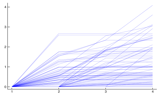
Figure 6: Scenarios of a running maximum process in four stages

Fig. 7 below shows two scenario trees with branching structure $(1,2,2,2)$ and $(1,3,3,3)$ approximating this process. They are generated with tree_approximation() function contained in the package ScenTrees.jl.¹

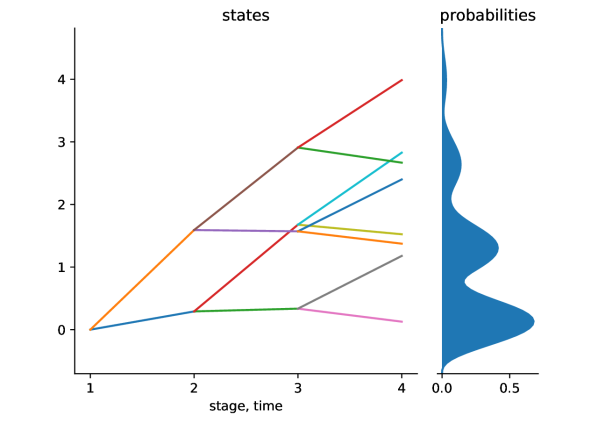
(a) Binary tree approximating process in Fig. 6 with a transportation distance of $0.313$

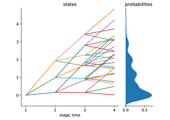
(b) Tree with 3 branches at each node approximating process in Fig. 6 with a transportation distance of $0.107$

Figure 7: Example of two scenario trees with different branching structures approximating process in Fig. 6.

Fig. 7(b) has a better approximating quality than Fig. 7(a). This is because Fig. 7(b) has more branches than Fig. 7(a) and therefore represents much more information. This can also be seen through the difference in the multistage distance. The multistage distance between the origin maximum running process $M_{t}$ (with realization in Fig. 6) and Fig. 7(b) is $0.107$ while that of Fig. 7(a) is $0.313$.

4 Scenario tree generation with limited data

In real world applications it is not unusual that data available is limited, i.e., that the number of available samples $N$ is fixed and not large; Rios et al. (2015) report further on this difficulty. To generate a stochastic tree based on limited data it is necessary to modify the approach in comparison to the Section 3 above. In these previous sections we combine and compress scenarios with similar outcomes at each step to locate new, continuative nodes of the tree. These methods need many, or unlimited data to specify a good approximating tree, and thus cannot be applied in case of limited data.

In case of limited data it is necessary to learn as much as possible from the observations available. The methods presented below differ in the problem already mentioned in Section 3, that is, how to deal with a specific history, which is not exactly met by any data observed.

To overcome this intrinsic difficulty we generate new and additional, but different samples based on the fixed number of observed samples $\xi_{j}$, $j=1,\dots N$, available. This is accomplished by estimating the density describing the transition.

These additional samples can then be used to apply the procedures outlined above, but in what follows we describe further algorithms which make direct use of the estimated transition distributions as well.

4.1 Scenario generation from limited data

In contrast to nested clustering (cf. Section 3) we estimate the distribution of the transition given the precise history. This distribution can be estimated by non-parametric kernel density estimation. That is, the density at stage $t+1$ conditional on the history $x_{[t]}:=(x_{1},x_{2},\dots,x_{t})$ is estimated by

$$\hat{f}_{t+1}(x_{t+1}\mid x_{[t]})=\sum_{j=1}^{N}w_{j}(x_{[t]})\cdot k_{h_{N}}\Big{(}x_{t+1}-\xi_{j,t+1}\Big{)},$$ (9)

where $k(\cdot)$ is a kernel function, $h_{N}$ is the bandwidth and $k_{h_{N}}(\cdot):=\frac{1}{h_{N}^{m_{t+1}}}k\left(\frac{\cdot}{h_{N}}\right)$. The weights

$$w_{j}(x_{[t]})=\frac{k\left(\frac{x_{i_{1}}-\xi_{j,1}}{h_{N}}\right)\cdot\ldots\cdot k\left(\frac{x_{i_{t}}-\xi_{j,t}}{h_{N}}\right)}{\sum_{\ell=1}^{N}k\left(\frac{x_{i_{1}}-\xi_{\ell,1}}{h_{N}}\right)\cdot\ldots\cdot k\left(\frac{x_{i_{t}}-\xi_{\ell,t}}{h_{N}}\right)}$$ (10)

depend on the history $x_{[t]}$ (for consistency, we set $w_{j}(x_{[1]}):=\frac{1}{N}$ for $t=1$).

It can be shown that the approximation is asymptotically optimal for
$h_{N}\sim N^{-1/(m_{1}+\dots+m_{t}+4)}$ (cf. Silverman’s rule of thumb, see also Pflug and Pichler (2016)). Note as well that the weights sum to $1$ in (10) ,i.e., for every $x_{[t]}$, $\sum_{j=1}^{N}w_{j}(x_{[t]})=1$. Further note that the estimator (9) for the conditional density involves all samples $\xi_{j}$, $j=1,\dots,N$. The weight $w_{j}(x_{[t]})$ is further large, if the first $t$ stages $(\xi_{j,1},\dots,\xi_{j,t})$ of the observation $\xi_{j}$ are similar to $x_{[t]}$, and negligible otherwise. In this way the weight $w_{j}(x_{[t]})$ determines the importance of the corresponding observation $\xi_{j}$ for $x_{[t]}$, and the estimator (9) takes this information adequately into account.

Univariate Kernel functions, which have proven useful are the Epanechnikov kernel $k(x)=\max\left\{\frac{3}{4}(1-x^{2}),\,0\right\}$ and the logistic kernel $k(x)=\frac{2}{(e^{x}+e^{-x})^{2}}$, cf. Tsybakov (2008). For multivariate data (i.e. higher dimension, $m_{t}>1$) univariate kernels can be multiplied to obtain a multivariate kernel function, $k(x_{1},\dots,x_{m_{t}})=k(x_{1})\cdot\ldots\cdot k(x_{m_{t}})$.

Samples from the conditional distribution (9) — the composition method.

The composition method allows to quickly find samples from the conditional distribution $f_{t+1}(\,\cdot\,|\,x_{[t]})$ in (9). Indeed, pick a random number $U\in(0,1)$, where $U$ is uniformly distributed. Then there is a summation index $j^{*}\in\{1,2,\dots N\}$ so that

$$\sum_{j=1}^{j^{*}-1}w_{j}(x_{[t]})<U\leq\sum_{j=1}^{j^{*}}w_{j}(x_{[t]}).$$ (11)

Note, that $j^{*}$ is distributed on $\{1,2,\dots N\}$ with probability mass function $P(j^{*}=j)=w_{j}(x_{[t]})$. For this index $j^{*}$ then randomly pick an instant from the kernel density $\frac{1}{h_{N}^{m_{t+1}}}k\left(\frac{\,\cdot\ \,-\xi_{j^{*},t+1}}{h_{N}}\right)$ shifted to $\xi_{j^{*},\,t+1}$, cf. (9). This sample is finally distributed with the desired density $\hat{f}_{t+1}(\,\cdot\,|\,x_{[t]})$. The composition method thus is a simple, quick and cheap method to make samples from the additively composed density (9) accessible.

4.2 A direct tree generation approach with limited data

Note that (9) describes a continuous distribution. To specify the tree process we may approximate the distribution again by finding a discrete distribution with locations and corresponding weights, which approximate (9) adequately.

A scenario tree can be generated directly by exploiting the conditional density estimates introduced above. To this end approximate the distribution in (9) with density $\hat{f}_{1}(\cdot)$ by the discrete distribution $\sum_{\ell\in\mathcal{S}_{1}}\tilde{p}_{\ell}\cdot\delta_{\tilde{x}_{\ell}}$ located at $\tilde{x}_{\ell}$ ($\ell\in\mathcal{S}_{1}$), where each $\tilde{x}_{\ell}$ is reached with probability $\tilde{p}_{\ell}$. These locations constitute the states at stage $t=1$, building the origin of the approximating tree.

For the next step define $\mathbf{\tilde{x}}_{i_{1}}:=(\tilde{x}_{i_{1}},\tilde{x}_{i_{2}})$ and consider the distribution with density $f_{1}(\cdot|\,\mathbf{\tilde{x}}_{i_{1}})$. By applying the same approximation procedure again one finds a discrete, approximating distribution $\sum_{\ell\in\mathcal{S}_{i_{1}}}p_{\ell}\cdot\delta_{\tilde{x}_{\ell}}$. The tree then is continued with $(\tilde{x}_{i_{1}},\tilde{x}_{i_{2}},\tilde{x}_{i_{3}})$, where $i_{2}\in\mathcal{S}_{i_{1}}$ is a successor of $i_{1}$.

A tree is finally found by repeatedly applying the method outlined above at every node in the subtree already available.

Input: Samples $\xi_{j}$ with $j=1,\ldots,N$ and a kernel function $k(\cdot)$

Output: A random vector $x=(x_{1},\ldots,x_{T})$ following the distribution in (9)

1 Initialization: $w=(1.0,\ldots,1.0)$ is an $N$-dimensional vector of sample weights, cf. (10).

2 for $t=1,\ldots,T$ do

3       Normalize the weights, set $w_{j}=\frac{w_{j}}{\sum_{\ell=1}^{N}w_{\ell}}$.

4       Set the bandwidth $h_{t}=\sigma_{t}\cdot N_{t}^{-\frac{1}{m_{t}+4}}$, where $m_{t}$ is the dimension, $N_{t}=\frac{\big{(}\sum_{j=1}^{N}w_{j}\big{)}^{2}}{\sum_{j=1}^{N}w_{j}^{2}}$ is the effective sample size and $\sigma_{t}^{2}=\operatorname{\mathsf{var}}\big{(}\xi_{j,t}\colon j=1,\ldots,N\big{)}$ is the variance at stage $t$.

5       Draw a uniform random number $U\in[0,1]$.

6       Find an index $j^{\ast}$ such that $\sum_{j=1}^{j^{\ast}-1}w_{j}<U\leq\sum_{j=1}^{j^{\ast}}w_{j}$ (cf. (11)).

7       Pick a random instance $K_{t}$ from the distribution with density $k(\cdot)$ and set $x_{t}=\xi_{j^{\ast},t}+h_{t}\cdot K_{t}$.

8       Re-calculate the sample weights for the next stage:

9       if Markovian then

10             for $j=1,\ldots,N$ do

11                  $w_{j}=k_{h_{t}}(x_{t}-\xi_{j,t})$

12            

13      else

14             for $j=1,\ldots,N$  do

15                  $w_{j}=w_{j}\cdot k_{h_{t}}(x_{t}-\xi_{j,t})$

16            

17      

Result: A random trajectory $(x_{1},\dots,x_{T})$ following the distribution (9)

Algorithm 2 Generate a new trajectory using conditional density estimation. ScenTrees.jl¹ provides this function as kernel_scenarios().

4.3 Stochastic approximation with limited data

The stochastic approximation algorithm outlined in Section 3.4 bases on additional sample paths, and each new sample path is used to improve the scenario tree. To obtain convergence of the method it is necessary to have an unlimited number of sample paths available, but this is certainly not the case for a limited number of data. However, the conditional density estimation methods described in this section allow generating new sample paths (cf. also Härdle et al. (1997)).

New sample paths from observations.

Every new sample path starts with $x_{1}$ at the first stage. Using (9) and the composition method one may find a new sample $x_{2}$ from $\hat{f}_{2}(\cdot\mid x_{[}1])$ at the second stage. Then generate another sample $x_{3}$ from $\hat{f}_{3}(\cdot\mid x_{[2]})$ at the third stage, a new sample $x_{t}$ from $\hat{f}_{t}(\cdot\mid x_{[t-1]})$ at the stage $t$, etc. Iterating the procedure until the final stage $T$ reveals a new sample path $x=(x_{1},x_{2},\dots,x_{T})$, generated from the initial data $\xi_{1},\dots,\xi_{N}$ directly (cf. Algorithm 2).

Generating new scenario paths can be repeated arbitrarily often to get new, distinct scenario paths. Each new sample path $x$ can be handed to the stochastic approximation algorithm (Section 3.4) to improve iteratively a tentative, approximating tree.

With this modification the stochastic approximation algorithm in Section 3.4 is eligible even in case of limited data.

Example 2 (Running Maximum using Algorithm 2).

Consider a case where we have just $N=100$ scenarios of running maximum data. We use this limited data and learn as much as possible so that we can generate new and additional samples based on this data. These generated samples are fed directly into stochastic approximation procedure to generate a scenario tree. Fig. 8 shows 100 trajectories generated from the data using Algorithm 2 and the resulting scenario tree with a branching structure of $(1,3,3,3)$.

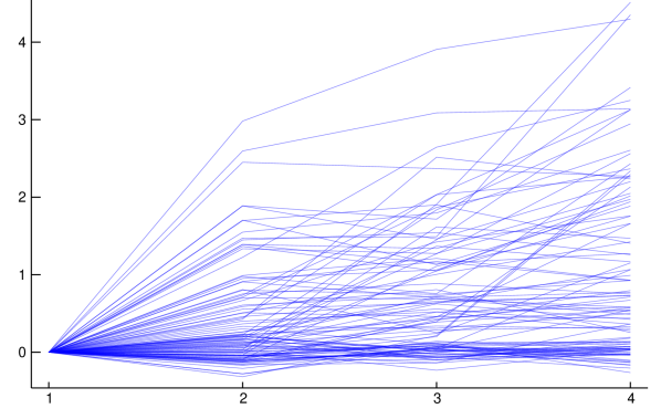
(a) 100 trajectories generated from the process in Fig. 6 using Algorithm 2

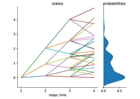
(b) Tree with 3 branches at each node approximating process in Fig. 8(a) with distance of $0.114$

Figure 8: 100 trajectories generated from a limited running maximum data and a resulting scenario tree, generated with ScenTrees.jl¹

It is clear that the data generated (cf. Fig. 8) is similar to the original data in Fig. 6. Therefore, this method proves efficient to generate new data for generation of scenario trees using stochastic approximation procedure (cf. Fig. 8(b)).

5 Generation of scenario lattices

In many situations of practical relevance the process to be approximated by a tree is known to have special properties. Of course, this information should be exploited when constructing the approximating tree in order to reduce the computational effort and time, and to obtain trees with better approximation quality.

In what follows we discuss the situations of Markovian processes and processes with fixed states separately. A main characteristic of trees in finance is arbitrage. For this we discuss arbitrage opportunities as well, and we provide a new result for trees with stochastic dominance in addition.

5.1 Markovian processes and lattices

Estimating a lattice follows the same principle as estimating a tree. However, the lattice generation procedure is of significantly lower complexity. If $D_{t}=\{\tilde{x}_{t,1},\dots,\tilde{x}_{t,i_{t}}\}$ is the set of states at stage $t$, then the induced distribution between the conditional lattice given $\tilde{x}_{t,i}$ and the Markovian process $\xi_{t}$ must be calculated only for all nodes from $D_{t}$ and not for all paths leading to them. As in the tree case, the calculation of the transport distance requires a backward algorithm but can be based on the approximation of the one-period transition probabilities $P(\xi_{t+1}\in A\mid\xi_{t}=x)$. The average aberration distance

$$\left(\operatorname{\mathds{E}}\left(\sum_{t=1}^{T}\,d_{t}\big{(}\xi_{t},\mathbf{T}_{t}(\xi_{t})\big{)}\right)^{r}\right)^{\nicefrac{{1}}{{r}}}$$ (12)

(cf. (2)) is an upper bound for the nested distance, but this upper bound may be conservative.

One has to consider the full conditional future process for the estimation of a scenario lattice, however, one does not have to consider the past. This fact allows the following simplifications for the algorithms:

1. When applying the nested clustering or stochastic approximation (Sections 3 and 3.4 above), for example, all samples can be reused at intermediate stages, as they do not have to have the same history.

2. When applying the density estimator (9), the weights in (10) simplify to

   $$w_{j}(x_{[t]})=\frac{k\left(\frac{x_{i_{t}}-\xi_{j,t}}{h_{N}}\right)}{\sum_{\ell=1}^{N}k\left(\frac{x_{i_{t}}-\xi_{\ell,t}}{h_{N}}\right)}.$$

Applications of lattice scenario models in an hydro storage management system can be found, e.g., in Löhndorf et al. (2013).

Example 3 (Gaussian random walk).

Consider the Gaussian random walk process $X_{n}=\sum_{k=1}^{n}Y_{k}$ on 5 stages, where the random variables $\big{(}Y_{k}\big{)}_{k\geq 1}$ are i.i.d. and the distribution of each $Y_{k}$ is normal. Simple examples of this process would be a path traced by a molecule as it travels through a liquid or a gas, the price of a fluctuating stock and the financial status of a gambler. Random walks are also simple representations of the Markov processes. Fig. 9 employs Algorithm 3 to approximate this process using a scenario lattice.

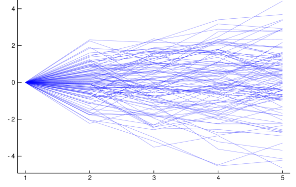
(a) 100 samples from Gaussian random walk process

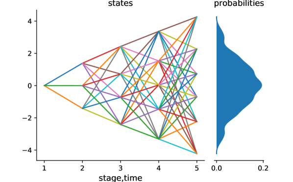
(b) Scenario lattice with branching structure $(1,3,4,5,6)$ approximating process in Fig. 9(a) with a distance of $0.554$

Figure 9: 100 samples from Gaussian random walk process and the resultant scenario lattice, generated with ScenTrees.jl

Input: Let $K$ be the number of iterations.

Output: Scenario lattice with values $\tilde{X}^{(K)}$ and transition probabilities.

1Initialization: Set the transportation distance $c_{E}=0$, set the counters $c(n)=0$ for all nodes and let $\tilde{X}^{(0)}$ be an initial lattice chosen by expert opinion, e.g. Also, choose a non-negative and non-increasing sequence $\alpha_{k}$ such that $\sum_{k=1}^{\infty}\alpha_{k}=\infty$ and $\sum_{k=1}^{\infty}\alpha_{k}^{2}<\infty$.

2 for $k=1,\ldots,K$ do

3       Use a new and independent trajectory $\xi^{(k)}=(\xi_{1}^{(k)},\ldots,\xi_{T}^{(k)})$

4       Find a scenario $s=(i_{1},\ldots,i_{T})$ of nodes with the closest lattice entry such that

$$i_{t}\in\operatorname*{\operatornamewithlimits{arg\,min}}_{n^{\prime}\in\mathcal{N}(t)}d_{t}\big{(}\tilde{X}^{(k)}(n^{\prime}),\xi_{t}^{(k)}\big{)},$$ (13)

where $\mathcal{N}(t)$ are all nodes in stage $t$.

5       for $t=1,\ldots,T$ do

6             Increase all counters $c(i_{t})=c(i_{t})+1$ for all nodes in $s$ (cf. (13)).

7             Modify the values of the nodes in these entries to be

$$\tilde{X}^{(k)}(i_{t})=\tilde{X}^{(k-1)}(i_{t})-\alpha_{k}\cdot r\cdot d_{t}\big{(}\tilde{X}^{(k-1)}(i_{t}),\xi_{t}^{(k)}\big{)}^{r-1}\cdot\big{(}\tilde{X}^{(k-1)}(i_{t})-\xi_{t}^{(k)}\big{)}.$$

The values on other node entries remain unchanged.

8      Set $c_{E}=c_{E}+\big{(}\sum_{t=1}^{T}d_{t}(\tilde{X}^{(k-1)}(i_{t}),\xi_{t}^{(k)})\big{)}^{r}.$

Result: Set the conditional probabilities $p(n)=\frac{c(n)}{K}$. The quantity approximating $\big{(}\operatorname{\mathds{E}}d(\xi,T(\xi))^{r}\big{)}^{\nicefrac{{1}}{{r}}}$ (cf. (12)) is given by $\big{(}c_{E}/K\big{)}^{\nicefrac{{1}}{{r}}}$.

Algorithm 3 Generating a scenario lattice with a fixed branching structure using stochastic approximation. ScenTrees.jl¹ provides this algorithm as lattice_approximation()

5.2 Processes with fixed states

In selected situations of practical relevance the distribution at stage $t$ is known approximately, or the support of this distribution or, for example, its quantiles can be described beforehand. In these situations it might make sense to fix the states beforehand and to use the algorithms introduced above to estimate the transition probabilities only, without modifying the states. Examples of such processes include mean reverting processes.

Figure 10: A scenario lattice process with fixed states

Figure 10 displays a scenario lattice with 5, fixed states, which do not change over time. The points $\tilde{x}_{2}$ to $\tilde{x}_{6}$ can be determined beforehand, and they are kept fixed over time. For a univariate distribution they can be chosen to be the quantiles, e.g. That is, $x_{2}$ is the $\nicefrac{{1}}{{10}}$-quantile, $x_{3}$ the $\nicefrac{{3}}{{10}}$-quantile, … and $x_{6}$ the $\nicefrac{{9}}{{10}}$-quantile, resp.

6 Trees lacking a predefined structure

Up to now we have assumed that the structure of the tree (i.e., the number of nodes and the predecessor vector $\operatorname{pred}$) has been chosen and is fixed. This a quite restrictive, since hardly anybody can decide beforehand what tree topology bes suits a given decision problem. Here is how to generate a tree with a given approximation quality without choosing the tree topology beforehand.

1. Choose (for each stage) a maximally acceptable distance between the estimated conditional densities and the discrete approximations.

2. Start with a simple tree (e.g., a binary one).

3. If during the tree construction the required distance cannot be achieved with the given number of successors, increase the branching factor by 1 until the distance condition can be satisfied.

Details of this procedure can be found in Pflug and Pichler (2014).

7 Application of scenario lattice generation methods to an electricity pricing data

To summarize the methods discussed in the preceding sections, we consider a limited electricity load data recorded for each hour of the day for the year 2017. The goal in what follows is to approximate the load of electricity for each hour of the day from this data using a scenario lattice. The scenario lattice has the same number of stages as the number of hours in the data. It also has a certain fixed branching structure (i.e., the number of nodes connected to each succeeding nodes in the lattice).

This computation has been done using the ScenTrees.jl¹ package which has been tested for Julia $\geq 1.0$.

Brief summary of the data.

The hourly actual load of electricity data consists of $52$ trajectories representing the $52$ weeks in a year (cf. Fig. 11). Each trajectory consists of the 7 days of the week. The data is recorded from $12\colon 00$ a.m. to $11\colon 59$ p.m. of each day. This means that we are employing a $52\times 168$ dimensional data where 168 stages represent the $24\times 7$ hours of each week.

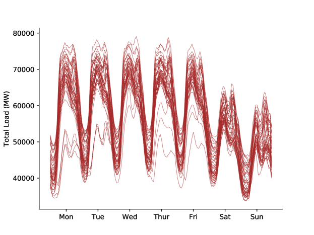
Figure 11: 52 trajectories of the data

The data shows a similar pattern in all the weeks. The actual total load of electricity tends to be higher during the weekdays than on the weekends. It is also higher during the daytime than in the nighttime. The maximum hourly mean of the data is $70\,290,4\text{\,}\mathrm{MW}$ and the minimum hourly mean is $38\,775,3\text{\,}\mathrm{MW}$. A special characteristic of the data is the presence of outliers which specifically represent holidays in Germany. For example, four of the holidays in the year 2017 fell on Monday (e.g., Easter Monday (April 17^th), Labor day (May 1^st), Whit day (June 5^th), Christmas (Dec 25^th)). These Monday-outliers are visible in Fig. 11.

7.1 Approximation by a scenario lattice

The data in Fig. 11 is limited. There are only $52$ trajectories in the data. We use the stochastic approximation procedure to discretize this data (Algorithm 3). Ideally, to obtain convergence of the stochastic approximation procedure, it is necessary to have an unlimited number of sample paths available. The step size $\alpha_{k}=\frac{1}{3000+k}$, where $k$ is the stochastic approximation iteration, turned out to be useful for this data.

Based on this data and using Algorithm 2, Fig. 12 shows a sample of new and additionally generated scenarios.

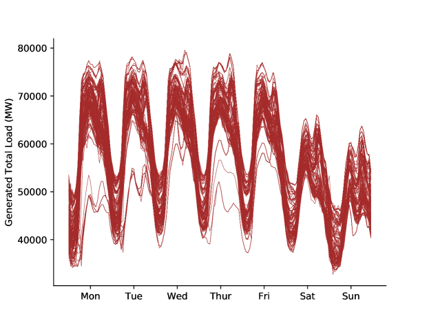
Figure 12: $1000\text{\,}\mathrm{n}$ew trajectories generated from the sample in Fig. 11 by employing Algorithm 2

These generated trajectories follow the same pattern as in the original data (cf. Fig. 11). All the important and necessary characteristics of the original sample is also captured in this data. Therefore, these trajectories totally represent the original sample without any loss of information.

To use ScenTrees.jl¹ we fix the branching structure of the approximating scenario lattice and the number of iterations. In this case, we generate a scenario lattice with 5 nodes at each stage and $2.0\times 10^{6}$ iterations.

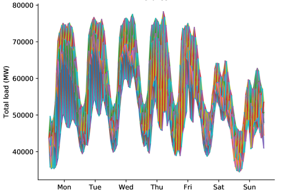
(a) Energy demand during the entire week

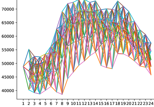
(b) Detailed, hourly view of Saturday

Figure 13: Scenario lattice generated from Fig. 11 using Algorithm 2 and Algorithm 3

The scenario lattice in Fig. 13 has $5$ branches connected to each node in each stage. There are a total of $836$ nodes and approximately $5.4\times 10^{116}$ scenarios possible in this lattice.

It is important to note that the generated scenario lattice is able to represent almost all the characteristics in the original data in Fig. 11. This lattice recognizes the patterns in the original data and is able to discretize the data and recover this pattern. To determine the quality of approximation of the scenario lattice, we employ the transportation distance (cf. (12)). Ideally, one would want to find a scenario lattice which minimizes this distance. The generated scenario lattice in Fig. 13 has a transportation distance of $1,203\text{\,}\mathrm{MW}$ per stage.

8 Conclusions

In this paper, we present new and fast implementations to generate scenario trees and scenario lattices for decision making under uncertainty. The package

ScenTrees.jl¹

collects efficient and freely available implementations of all algorithms. We also provided explicit concepts to measure the quality of the approximation by employing distances, particularly the transportation distance. This distance constitutes an essential tool in stochastic optimization. We introduce several techniques to constructively obtain scenario tress from samples, which are observed trajectories. We particularly elaborate on methods to find scenario trees and lattices with limited data only. We specifically apply scenario lattice generation methods on a limited electricity load data.

Our results prove that the new algorithms for generating scenario trees and scenario lattices are important as they are able to discretize the data such that all the information in the data is captured. These results also show that our implementation is highly competitive in terms of computational performance.

Appendix A The Kantorovich/ Wasserstein distance

Recall the definition of the Kantorovich/ Wasserstein distance $\mathsf{d}_{r}(P,\tilde{P})$ of order $r$ for two (Borel) random measures $P$ and $\tilde{P}$ on $\mathbb{R}^{m}$:

$$\mathsf{d}_{r}(P,\tilde{P}):=\inf_{\pi} \left(\iint_{\mathbb{R}^{m}\otimes\mathbb{R}^{m}}\|\xi-\tilde{\xi}\|^{r}\,\pi(\mathrm{d}\xi,\mathrm{d}\tilde{\xi})\right)^{1/r}$$

s.t. $$\pi\left(A\times\mathbb{R}^{m}\right)=P(A)$$ (14)

$$\pi\left(\mathbb{R}^{m}\times B\right)=\tilde{P}(B).$$ (15)

The infimum is over all Borel measures $\pi$ on $\mathbb{R}^{m}\times\mathbb{R}^{m}$ with given marginals $P$ and $\tilde{P}$. These measures are called transportation plans. If $X$ and $\tilde{X}$ are $\mathbb{R}^{m}$-valued random variables, then their distance is defined as the distance of the corresponding image measures $P^{X}$ and $P^{\tilde{X}}$.

The Kantorovich/ Wasserstein distance does not always have a representation via a transportation map. If, however, $P$ is atomless on a separable space $\Xi$, then it can be employed to approximate any measure in Kantorovich/ Wasserstein distance arbitrarily close via a transport plan. I.e., for every measure $\tilde{P}$ on $\tilde{\Xi}$ and $\varepsilon>0$ there is a transport map $T\colon\Xi\to\tilde{\Xi}$ such that

$$\mathsf{d}\big{(}\tilde{P},P^{T}\big{)}<\varepsilon\ \text{ and }\ \mathsf{d}\big{(}P^{T},P\big{)}<\mathsf{d}(\tilde{P},P)+\varepsilon.$$

To accept the assertion recall from Bolley (2008) that there are discrete measures $P_{n}=\sum_{i=1}^{n}p_{i}\delta_{x_{i}}$ and $\tilde{P}_{m}=\sum_{j=1}^{m}\tilde{p}_{j}\delta_{y_{j}}$ such that $\mathsf{d}(P,P_{n})<\varepsilon/2$ and $\mathsf{d}(\tilde{P},\tilde{P}_{m})<\varepsilon/2$. Further, there is a Dirichlet tessellation of $\Xi$ in disjoint sets, $\Xi=\dot{\bigcup}_{i=1}^{n}\Xi_{i}$, such that

$$\Xi_{i}\subset\{\xi\colon d(\xi,x_{i})\leq d(\xi,x_{i^{\prime}})\text{ for all }i^{\prime}=1,\dots,n\}$$

and without loss of generality we may assume that $p_{i}=P(\Xi_{i})$.

Let $\pi$ denote the transport plan so that $\mathsf{d}(P_{n},\tilde{P}_{m})=\sum_{i=1}^{n}\sum_{j=1}^{m}d(x_{i},y_{j})\pi_{i,j}$, satisfying the marginal constraints (14) and (15), i.e., $p_{i}=\sum_{j=1}^{m}\pi_{i,j}$ and $\tilde{p}_{j}=\sum_{i=1}^{n}\pi_{i,j}$. As $P$ does not give masses to atoms, one may dissect the sets $\Xi_{i}=\dot{\bigcup}_{j=1}^{m}\Xi_{i,j}$ so that $P(\Xi_{i,j})=\pi_{i,j}$. It holds that $\Xi=\dot{\bigcup}_{i=1,j=1}^{n,\ \ m}\Xi_{i,j}$, so that the transport map

$$T(x):=y_{j}\text{ if }x\in\Xi_{i,j}$$

is well defined. By construction, $P^{T}=\tilde{P}_{m}$, so that $\mathsf{d}(\tilde{P},P^{T})<\varepsilon$ and $\mathsf{d}(P,P^{T})<\mathsf{d}(P,\tilde{P})+\varepsilon$.

$$\mathsf{d}(\tilde{P},P^{T})\leq\mathsf{d}(\tilde{P},\tilde{P}_{m}),$$

the assertion.

Appendix B The nested distance

The nested distance introduced in Pflug (2009); Pflug and Pichler (2012) generalizes the Kantorovich/ Wasserstein distance. Its definition given in (16)–(18) above is for the laws of stochastic processes, the image measures on filtered probability spaces.

The following mathematical definition of the nested distance generalizes the recursive description above. It is an obvious generalization of the Wasserstein distance, which Appendix A elaborates in detail. The nested distance, denoted $\mathsf{d\kern-0.70007ptl}$, is

$$\inf_{\pi}\operatorname{\mathds{E}}_{\pi}d(\xi,\eta) =\iint_{\Xi^{T}\times\Xi^{T}}d(\xi,\eta)\,\pi(\mathrm{d}\xi,\mathrm{d}\eta)$$ (16)

subject to $$\pi(A\times\Xi^{T}\mid\mathcal{F}_{t}\times\mathcal{F}_{t})=P(A\mid\mathcal{F}_{t}),\quad A\in\mathcal{F}_{T}\text{ and }$$ (17)

$$\pi(\Xi^{T}\times B\mid\mathcal{F}_{t}\times\mathcal{F}_{t})=Q(B\mid\mathcal{F}_{t}),\quad B\in\mathcal{F}_{T}$$ (18)

$$\qquad\qquad\text{ for all stages }t\in\{1,\dots,T\},$$

where the infimum is among all bivariate probability measures $\pi$ satisfying the marginal constraints (17) and (18) at all stages $t\in\{1,\dots,T\}$.

We note that for random variables, or stochastic processes in one stage, the definition of the nested distance (16)–(18) coincides with the Wasserstein or Kantorovich distance. Both are transportation distances, but the nested distance additionally takes the evolving information into account via (17) and (18).

The construction principle of the nested distance is (backwards) recursive. To compute the nested distance of two trees of same height we isolate the roots from the tree and consider the root, and all remaining subtrees separately:

1. The root nodes of both trees have a specified distance, which is available by employing the distance $d_{t}$ at the stage $t$.

2. Each successor node of the root node is the root node of a subtree. Further, a transition probability from the root node to each subtree is available by employing the transportation distance, applied do the subtrees.

   Each combination of subtrees from both trees has a nested distance, which is available by recursion. These nested distances of subtrees constitute (abstract) costs. The transportation distance, as specified above, makes a distance of the successor nodes (i.e., subtrees) available.

The nodes at the final stage $t=T$ do not have subtrees, such that the component (ii) does not apply at stage $t=T$: by (i), the nested distance is $d_{T}$ at stage $t=T$. The nested distance of intermediate trees at the same stage is given by recombining the roots and the subtrees, i.e., the nested distance is (i) + (ii).

The nested distance finally is the distance of the trees from their root node $0$ and available in a backwards recursive way.

To interpret this definition, the nested distance between two multistage probability distributions is obtained by minimizing over all transportation plans $\pi$ transporting one distribution into the other, which are compatible with the filtration structures in addition. For a single period, i.e. $T=1$, the nested distance coincides with the Kantorovich/ Wasserstein distance. The nested distance is crucial for multistage stochastic optimization by the following theorem on stability of stochastic multistage optimization problems (cf. Pflug and Pichler (2012)).

Theorem 4.

Let $\mathbb{P}:=(\Xi,(\mathcal{F}_{t})_{t=1}^{T},P)$ ($\tilde{\mathbb{P}}$, resp.) be a filtered probability space. Consider the multistage stochastic optimization problem

$$v(\mathbb{P}):=\inf\left\{\operatorname{\mathds{E}}_{\xi}^{\mathbb{P}}\big{(}Q(\xi,x)\big{)}\colon x\lhd\mathcal{F}\right\},$$

where $Q$ is convex in the decisions $x=(x_{1},\dots,x_{T})$ for any $\xi$ fixed, and Lipschitz with constant $L$ in the scenario process $\xi=(\xi_{1},\dots,\xi_{T})$ for any $x$ fixed. The constraint $x\lhd\mathcal{F}$ means that the decisions can be random variables, but must be adapted to the filtration $\mathcal{F}$, i.e., must be nonanticipative. Then the objective values $v(\mathbb{P})$ and $v(\tilde{\mathbb{P}})$ calculated with the two different probability models for the scenario process $\mathbb{P}$ and $\tilde{\mathbb{P}}$, satisfy

$$\left|v(\mathbb{P})-v(\tilde{\mathbb{P}})\right|\leq L\cdot\mathsf{d\kern-0.70007ptl}(\mathbb{P},\tilde{\mathbb{P}})\,.$$

March 8, 2024, TreeGeneration2020.pdf

References

- Bally et al. (2005) V. Bally, G. Pagès, and J. Printems. A quantization tree method for pricing and hedging multidimensional American options. Mathematical Finance, 15(1):119–168, 2005. doi:10.1111/j.0960-1627.2005.00213.x.
- Bellman (1961) R. E. Bellman. Adaptive control processes. Princeton Legacy Library 2045. Princeton University Press, 1961. ISBN 978-1-4008-7466-8. doi:10.1002/nav.3800080314.
- Beyer et al. (2014) H.-G. Beyer, S. Finck, and T. Breuer. Evolution on trees: On the design of an evolution strategy for scenario-based multi-period portfolio optimization under transaction costs. Swarm and Evolutionary Computation, 17:74–87, 2014. doi:10.1016/j.swevo.2014.03.002.
- Bolley (2008) F. Bolley. Separability and completeness for the Wasserstein distance. In C. Donati-Martin, M. Émery, A. Rouault, and C. Stricker, editors, Séminaire de Probabilités XLI, volume 1934 of Lecture Notes in Mathematics, pages 371–377. Springer, Berlin, Heidelberg, 2008. doi:10.1007/978-3-540-77913-1.
- Consigli et al. (2000) G. Consigli, J. Dupačová, and S. W. Wallace. Generating scenarios for multistage stochastic programs. Ann. Oper. Res., 100:25–53, 2000. doi:10.1023/A:1019206915174.
- Dantzig (1955) G. B. Dantzig. Linear programming under uncertainty. Management Science, 1(3 and 4):197–206, 1955.
- Dudley (1969) R. M. Dudley. The speed of mean Glivenko-Cantelli convergence. The Annals of Mathematical Statistics, 40(1):40–50, 1969.
- Fairbrother et al. (2015) J. Fairbrother, A. Turner, and S. W. Wallace. Scenario generation for stochastic programs with tail risk measures, 2015. URL https://arxiv.org/abs/1511.03074.
- Graf and Luschgy (2000) S. Graf and H. Luschgy. Foundations of Quantization for Probability Distributions, volume 1730 of Lecture Notes in Mathematics. Springer-Verlag, Berlin, 2000. doi:10.1007/BFb0103945.
- Hanasusanto et al. (2015) G. A. Hanasusanto, V. Roitch, D. Kuhn, and W. Wiesemann. A distributionally robust perspective on uncertainty quantification and chance constrained programming. Mathematical Programming, 151(1):35–62, 2015. doi:10.1007/s10107-015-0896-z.
- Härdle et al. (1997) W. Härdle, H. Lütkepohl, and R. Chen. A review of nonparametric time series analysis. International Statistical Review, 65(1):49–72, 1997. doi:10.2307/1403432.
- Hartigan (1975) J. A. Hartigan. Clustering Algorithms. Wiley New York, 1975.
- Heitsch and Römisch (2009) H. Heitsch and W. Römisch. Scenario tree modeling for multistage stochastic programs. Math. Program. Ser. A, 118:371–406, 2009. doi:10.1007/s10107-007-0197-2.
- Henrion and Römisch (2018) R. Henrion and W. Römisch. Problem-based optimal scenario generation and reduction in stochastic programming. Mathematical Programming, 2018. doi:10.1007/s10107-018-1337-6.