Equivalent Definitions of the Mie-Grüneisen Form

Abstract

We define the Mie-Grüneisen form in five different ways, then demonstrate their equivalence.

I Introduction

Equations of state (EOS) often are described as being of Mie-Grüneisen (MG) form, or type. This is usually meant to convey that the pressure relative to that of some reference curve (subscripted ‘0’) can be derived from the energy relative to that curve via

$$P(V,T)-P_{0}(V)=\frac{\Gamma(V)}{V}[E(V,T)-E_{0}(V)],$$ (1)

where the Grüneisen parameter $\Gamma$ is a function of volume only. MG EOS appear frequently in high-pressure and -temperature physics. They are particularly useful when applied to materials for which a single locus (such as the principal Hugoniot or isentrope) is well-characterized experimentally, with far fewer or lower-quality data elsewhere. This is true of many materials with shock data recorded in the LASLMarsh (1980) and LLNLvan Thiel, Shaner, and Salinas (1977) compendia, as well as most high explosive (HE) product mixtures.poi Procedures for extracting the cold compression curve from shock data using Eq. (1) appeared very early in the history of shock physics,Benedek (1959); Rice, McQueen, and Walsh (1958) and fits of the Jones-Wilkins-Lee (JWL) formLee, Hornig, and Kury (1968) to cylinder expansion data can be made thermodynamically complete on the same basis.Menikoff (2015)

While the MG form often is defined through Eq. (1),Eliezer, Ghatak, and Hora (2002) additional statements (discussed below) have been derived as consequences. Aside from the question as to whether (1) is actually overdetermined (i.e., redundant), many discussions implicitly suggest its primacy by the order in which alternative expressions are presented, as if they were merely its consequences.

Our purpose here is to clarify the precise relationship between various formulae that have appeared in discussions of the MG form. Specifically, we will define the form in five different ways that do not include (1), then demonstrate their complete equivalence. Each pairwise relationship is one of mutual entailment, meaning that any single definition is sufficient to prove the others and that primacy cannot be assigned to any individual. Because no one definition is independent or unique, its emphasis in a particular context is purely a matter of convenience. Some of these results are well-known and have appeared elsewhere (at most depth in Ref. Menikoff, 2016), but we are aware of no previous attempts to so explicitly make these connections clear.

The following section introduces the definitions, their equivalence is proven in Sec. III, and in Section IV we discuss some implications.

II Definitions

The following five definitions of the MG form are equivalent, meaning that any one serves as the necessary and sufficient condition for any other. Not every definition is expressed in a single equation, so definitions will be distinguished from equation numbers by a prepended ‘#’.

Definition #1

The first definition is a slight generalization of (1),

$$P(V,T)-P_{0}(V)=\frac{\Gamma}{V}[E(V,T)-E_{0}(V)],$$ (2)

where subscripts have the same meaning as before and $\Gamma$ is the Grüneisen parameter defined by

$$\Gamma=V\left(\frac{\partial P}{\partial E}\right)_{V}=-\frac{V}{T}\left(\frac{\partial T}{\partial V}\right)_{S}.$$ (3)

Unlike (1), #1 imposes no restriction on the state-dependence of $\Gamma$ (viz., that it is a function only of $V$).

Definition #2

In general, the Grüneisen parameter as defined by Eq. (3) is an arbitrary function of the thermodynamic state. In the MG form, it is a function of volume only,

$$\Gamma=\Gamma(V).$$ (4)

Definition #3

The entropy,

$$S=f(x),$$ (5)

is a function only of the scaled temperature, $x=T/\Theta(V)$. The scaling factor $\Theta(V)$ is usually a characteristic temperature such as that of Debye or EinsteinMcQuarrie (1975) and is, at most, a function of $V$.

Definition #4

The heat capacity at constant volume,

$$C_{V}=\left(\frac{\partial E}{\partial T}\right)_{V}=T\left(\frac{\partial S}{\partial T}\right)_{V},$$ (6)

is a function only of the entropy,

$$C_{V}=C_{V}(S).$$ (7)

Definition #5

The temperature- and volume-dependencies of the Helmholtz free energy can be decomposed as

$$A(V,T)=\phi(V)+\Theta(V)f(x),$$ (8)

where $f(x)$ and $\phi(V)$ are single-argument functions that are otherwise arbitrary, and the same comments apply to $x=T/\Theta(V)$ as in (5). The first term on the right hand side is an internal energy as well as a free energy.

III Equivalence

Each of the following subsections demonstrates equivalence of a pair of definitions drawn from the five given above. Specifically, we consider four different pairs indicated by the arrows in Figure 1. This diagram is complete in the sense that any definition follows from any other, either directly (e.g., #2$\rightarrow$#4) or via one additional step (e.g., #3$\rightarrow$#2$\rightarrow$#1). More arrows could readily be drawn, (e.g., #3$\rightarrow$#1), but we have opted for a sufficient set based on what seemed to be the simplest proofs. We also wish to emphasize that the topology of Figure 1 should not be misconstrued to assign any conceptual significance to #2, but merely reflects the convenience of its use.

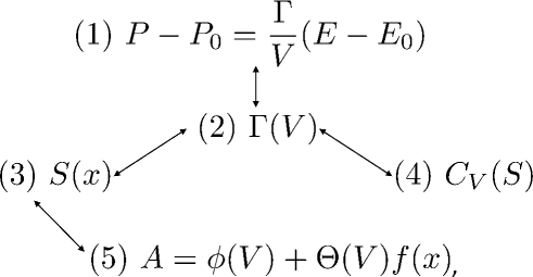
Figure 1: Five definitions of the Mie-Grüneisen form, with arrows indicating demonstrations of equivalence provided in the text. $\Gamma$ satisfies (3), and $x=T/\Theta(V)$.

III.1 #1 $\xleftrightarrow{}$ #2

Differentiation of Eq. (2) with respect to $T$ at constant $V$ produces

$$\left(\frac{\partial P}{\partial T}\right)_{V}=\left(\frac{\partial\Gamma}{\partial T}\right)_{V}\frac{\left[E(T,V)-E_{0}(V)\right]}{V}+\frac{\Gamma}{V}C_{V}.$$ (9)

The left-hand-side (lhs) of (9) can also be evaluated using the chain rule in combination with Eqs. (3) and (6),

$$\left(\frac{\partial P}{\partial T}\right)_{V}=\left(\frac{\partial P}{\partial E}\right)_{V}\left(\frac{\partial E}{\partial T}\right)_{V}=\frac{\Gamma}{V}C_{V}.$$ (10)

Equality of Eqs. (9) and (10) requires that $\left(\frac{\partial\Gamma}{\partial T}\right)_{V}=0$, establishing that #2 follows from #1.

Conversely, integrating Eq. (10) with respect to $T$ at constant $V$ under the assumption that $\Gamma/V$ is a function of $V$ only (definition #2) produces

$$P=\frac{\Gamma}{V}E+C(V).$$ (11)

Taking $C(V)=P_{0}(V)-\frac{\Gamma(V)}{V}E_{0}(V)$ for some reference curve $\{P_{0}(V),E_{0}(V)\}$ produces Eq. (2). Definition #2 thereby entails #1.

III.2 #2 $\xleftrightarrow{}$ #3

We first demonstrate #3$\rightarrow$#2. The Grüneisen parameter can also be written in terms of observables asMenikoff and Plohr (1989)

$$\Gamma=\frac{V\alpha B_{T}}{C_{V}},$$ (12)

where $\alpha$ is the volumetric expansion coefficient,

$$\alpha=\frac{1}{V}\left(\frac{\partial V}{\partial T}\right)_{P},$$ (13)

and $B_{T}$ is the isothermal bulk modulus,

$$B_{T}=-V\left(\frac{\partial P}{\partial V}\right)_{T}.$$ (14)

Based on definition #3, the denominator of (12) is

$$C_{V}=T\left(\frac{\partial S}{\partial T}\right)_{V}=x\frac{dS}{dx},$$ (15)

and the numerator is

$$V\alpha B_{T} =V\left(\frac{\partial P}{\partial T}\right)_{V}=V\left(\frac{\partial S}{\partial V}\right)_{T}$$

$$=V\frac{dS}{dx}\left(\frac{\partial x}{\partial V}\right)_{T}=-\frac{VT}{\Theta^{2}}\frac{dS}{dx}\frac{d\Theta}{dV}$$

$$=-x\frac{dS}{dx}\frac{d\ln\Theta}{d\ln V}.$$ (16)

The first of the equalities in (16) follows from the cyclic rule for partial differentiationMenikoff and Plohr (1989)

$$\left(\frac{\partial x}{\partial y}\right)_{z}\left(\frac{\partial z}{\partial x}\right)_{y}\left(\frac{\partial z}{\partial x}\right)_{y}=-1,$$ (17)

and the second from a Maxwell relation in the Helmholtz representation.Callen (1985) Substitution of (15) and (16) into (12) gives

$$\Gamma=-\frac{d\ln\Theta}{d\ln V},$$ (18)

a function only of $V$. This argument is very similar to that of Wallace,wal and is sufficient to prove that #2 follows from #3.

The converse, #2$\rightarrow$#3, is slightly more detailed. Again using the cyclic rule, the second definition of $\Gamma$ in (3) can be rewritten as

$$\Gamma(V)=-\frac{V}{T}\left(\frac{\partial T}{\partial V}\right)_{S}=\frac{V}{T}\left(\frac{\partial T}{\partial S}\right)_{V}\left(\frac{\partial S}{\partial V}\right)_{T},$$ (19)

or as a partial differential equation for the entropy,

$$\frac{V}{\Gamma(V)}\left(\frac{\partial S}{\partial V}\right)_{T}-T\left(\frac{\partial S}{\partial T}\right)_{V}=0.$$ (20)

Equation (20) can be solved by the method of characteristics, where the characteristics satisfy the following system of ordinary differential equations parameterized by $t$:

$$\frac{dV}{dt}=\frac{V}{\Gamma(V)}$$ (21)

$$\frac{dT}{dt}=-T$$ (22)

$$\frac{dS}{dt}=0.$$ (23)

The last of these demonstrates that the characteristic curves are isentropic, whereas the first two can be combined to eliminate $t$

$$\frac{dT}{T}+\frac{\Gamma(V)}{V}dV=0,$$ (24)

and then straightforwardly integrated via separation of variables, yielding

$$Te^{\int_{V_{0}}^{V}\frac{\Gamma(V^{\prime})}{V^{\prime}}dV^{\prime}}=C.$$ (25)

The solution to (20) is the union of all such curves (conveniently labeled by the integration constant $C$) and entropy can thus be expressed as

$$S=f(C)=f\left(Te^{\int_{V_{0}}^{V}\frac{\Gamma(V^{\prime})}{V^{\prime}}dV^{\prime}}\right)$$ (26)

for arbitrary function $f$. This expression is simply Eq. (5) with $\Theta(V)=e^{-\int_{V_{0}}^{V}\frac{\Gamma(V^{\prime})}{V^{\prime}}dV^{\prime}}$, thereby proving #2 $\rightarrow$ #3.

III.3 #2 $\xleftrightarrow{}$ #4

The equality of these statements was shown originally by DavisDavis (2000) and discussed in more detail by Menikoff.Menikoff (2016) It is based on the invariance of mixed third derivatives of $E(S,V)$ to the order in which they are taken (i.e., a higher-order analogue of the Maxwell relations). In this case,

$$\frac{\partial}{\partial V}\frac{\partial^{2}E}{\partial S^{2}}=\frac{\partial^{2}}{\partial S^{2}}\frac{\partial E}{\partial V},$$ (27)

which can be reexpressed as

$$-\frac{\Gamma}{V}\frac{T}{C_{V}}\left(\frac{\partial\Gamma}{\partial S}\right)_{V}=\frac{V}{C_{V}^{2}}\left(\frac{\partial C_{V}}{\partial V}\right)_{S}.$$ (28)

The lhs vanishes if $\Gamma$ is a function only of $V$, requiring that $C_{V}$ be a function only of $S$ and vice-versa.

III.4 #3 $\xleftrightarrow{}$ #5

That #5$\rightarrow$#3 follows from simple differentiation, $\left(\frac{\partial A}{\partial T}\right)_{V}=-S$. Conversely, integration of $S=f(T/\Theta(V))$ with respect to $T$ along some path of constant volume gives

$$A(T,V)-A_{0}(V)=\theta(V)g(T/\Theta(V)),$$ (29)

where $\frac{dg(x)}{dx}=-f(x)$. The function $g(x)$ is known up to an integration constant. Convenient choices for this constant include $g(0)=0$ and $\theta(V)g(0)=E_{ZP}$, where $E_{ZP}$ is the vibrational zero-point energy (zpe). The first results in $\left.A(V,T)\right|_{T=0}=A_{0}(V)$ equivalent to the zero-temperature isotherm, the second in its being the cold internal energy without zpe. The latter is often calculated using density functional theory,Martin (2004) and is sometimes referred to as the cold curve.Peterson et al. (2012)

IV Comments

• Definitions #1 and #2 often are combined as the single statement (1), when in fact this is redundant: #1$\leftrightarrow$#2 and so either alone is sufficient to fully define the MG form.

• It is sometimes convenient to generalize Eq. (1) to $\Gamma$ as a function of variables in addition to volume, such as internal energy or temperature.Bushman et al. (1993) This poses no difficulty so long as it is understood that the new $\Gamma(V,E)$ or $\Gamma(V,T)$ is not that defined by Eq. (3). For $\Gamma$ to satisfy both (2) and (3), it must also satisfy (4) because #1$\rightarrow$#2. See, for example, Eqs. (1a-b) and (2a-b) of Ref. Fumi and Tosi, 1962.

• If the entropy is invertible, then #4 can be recast in the (possibly more intuitive) form $C_{V}=C_{V}(x)$. Generally speaking, this should be true except at phase boundaries.

• We have restricted our discussion to various expressions of the MG form at the level of classical thermodynamics, without having considered the microscopic implications of their validity. The literature on this topic is vast, but the work most closely related to ours is Ref. Fumi and Tosi, 1962. Such considerations typically are framed in terms of what is required in order for #2 to hold.

• For systems poorly-described by a single characteristic temperature (e.g., polymersWunderlich (2005) or other molecular solids such as high explosivesCawkwell et al. (2017)), it is often convenient to express the free energy as a sum of non-interacting components,

  $$A(V,T)=\sum_{i}A_{i}(V,T),$$ (30)

  where each component free energy can be decomposed in the manner of (8). Fig. 1 and all proofs still apply separately to each component $i$. For example, the partial pressures are

  $$P_{i}-P_{i,0}=\frac{\Gamma_{i}}{V}[E_{i}-E_{i,0}],$$ (31)

  where $\Gamma_{i}=-V\frac{d\Theta_{i}(V)}{dV}$ and the total pressure $P=\sum_{i}P_{i}$. Note, however, that the thermodynamically consistent definition of $\Gamma$ is not the sum of $\Gamma_{i}$. Rather, the $\Gamma$ consistent with (3) and (12) is given by

  $$\Gamma=\frac{\sum_{i}C_{V,i}\Gamma_{i}}{\sum_{i}C_{V,i}},$$ (32)

  where

  $$C_{V}=\sum_{i}C_{V},i.$$ (33)

  Multiple characteristic temperature models can therefore be of MG form only if all characteristic temperatures have the same $\Gamma$.

References

- Lyon and Johnson (1992) S. P. Lyon and J. D. Johnson, “SESAME: The Los Alamos National Laboratory equation of state database,” Report LA-UR-92-3407 (Los Alamos National Laboratory, 1992).
- Marsh (1980) S. P. Marsh, ed., LASL Shock Hugoniot Data (University of CA Press, 1980).
- van Thiel, Shaner, and Salinas (1977) M. van Thiel, J. Shaner, and E. Salinas, “Compendium of Shock Wave Data,” Tech. Rep. UCRL-50108 (Lawrence Livermore Laboratory, 1977).
- (4) See the many JWL fits to principal release data found in Ref. dob, 1981.
- Benedek (1959) G. B. Benedek, “Deduction of the volume dependence of the cohesive energy of solids from shock-wave compression measurements,” Phys. Rev. 114, 467–475 (1959).
- Rice, McQueen, and Walsh (1958) M. Rice, R. McQueen, and J. Walsh, “Compression of solids by strong shock waves,” in Advances in Research and Applications, Solid State Physics, Vol. 6, edited by F. Seitz and D. Turnbull (Academic Press, 1958) pp. 1 – 63.
- Lee, Hornig, and Kury (1968) E. L. Lee, H. C. Hornig, and J. W. Kury, “Adiabatic expansion of high explosive detonation products,” Report UCRL-50422 (University of CA Radiation Laboratory, 1968).
- Menikoff (2015) R. Menikoff, “JWL equation of state,” Report LA-UR-15-29536 (Los Alamos National Laboratory, 2015).
- Eliezer, Ghatak, and Hora (2002) S. Eliezer, A. Ghatak, and H. Hora, Fundamentals of Equations of State (World Scientific Publishing Co. Pte. Ltd., 2002) pg. 153.
- Menikoff (2016) R. Menikoff, “Complete Mie-Grüneisen equation of state (update),” Report LA-UR-16-21706 (Los Alamos National Laboratory, 2016).
- McQuarrie (1975) D. A. McQuarrie, Statistical Mechanics (University Science Books, 1975) see Chapter 11.
- Menikoff and Plohr (1989) R. Menikoff and B. J. Plohr, “The Riemann problem for fluid flow of real materials,” Rev. Mod. Phys. 61, 75 (1989).
- Callen (1985) H. B. Callen, Thermodynamics and an Introduction to Thermostatistics (John Wiley & Sons, 1985).
- (14) Ref. Wallace, 1972, pg. 52.
- Davis (2000) W. C. Davis, “Complete equation of state for unreacted solid explosive,” Combustion and Flame 120, 399 – 403 (2000).
- Martin (2004) R. M. Martin, Electronic Structure:Basic Theory and Practical Methods (Cambridge University Press, 2004).
- Peterson et al. (2012) J. H. Peterson, K. G. Honnell, C. Greeff, J. D. Johnson, J. Boettger, and S. Crockett, “Global equation of state for copper,” AIP Conference Proceedings 1426, 763–766 (2012), https://aip.scitation.org/doi/pdf/10.1063/1.3686390 .
- Bushman et al. (1993) A. V. Bushman, M. V. Zhernokletov, I. V. Lomonosov, Y. N. Sutulov, V. E. Fortov, and K. V. Khishchenko, “Investigation of plexiglas and teflon under double shock waves loading and isentropic expansion. plastics equation of state at high energy density,” Dokl. Akad. Nauk SSSR 329, 581–584 (1993), (In Russian.).
- Fumi and Tosi (1962) F. Fumi and M. Tosi, “On the Mie-Grüneisen and Hildebrand approximations to the equation of state of cubic solids,” Journal of Physics and Chemistry of Solids 23, 395 – 404 (1962).
- Wunderlich (2005) B. Wunderlich, Thermal Analysis of Polymeric Materials (Springer, Berlin, 2005).
- Cawkwell et al. (2017) M. J. Cawkwell, D. S. Montgomery, K. J. Ramos, and C. A. Bolme, “Free energy based equation of state for pentaerythritol tetranitrate,” The Journal of Physical Chemistry A 121, 238–243 (2017), pMID: 27997195, https://doi.org/10.1021/acs.jpca.6b09284 .
- dob (1981) “LLNL Explosives Handbook, Properties of Chemical Explosives and Explosive Simulants,” Tech. Rep. UCRL-52997 (Lawrence Livermore National Laboratory, 1981).
- Wallace (1972) D. C. Wallace, Thermodynamics of Crystals (Dover Publications, Inc., 1972).