Measurements of undulator radiation power noise and comparison with ab initio calculations

Abstract

Generally, turn-to-turn fluctuations of synchrotron radiation power in a storage ring depend on the 6D phase-space distribution of the electron bunch. This effect is related to the interference of fields radiated by different electrons. Changes in the relative electron positions and velocities inside the bunch result in fluctuations in the total emitted energy per pass in a synchrotron radiation source. This effect has been previously described assuming constant and equal electron velocities before entering the synchrotron radiation source. In this paper, we present a generalized formula for the fluctuations with a non-negligible beam divergence. Further, we corroborate this formula in a dedicated experiment with undulator radiation in the Integrable Optics Test Accelerator (IOTA) storage ring at Fermilab. Lastly, possible applications in beam instrumentation are discussed.

I Introduction

Full understanding of the radiation generated by accelerating charged particles is crucial for accelerator physics and electrodynamics in general. The predictions of classical electrodynamics for pulse-by-pulse average characteristics of synchrotron radiation, such as the total radiated power, spectral composition, angular intensity distribution and brightness [1], are supported by countless observations. In fact, they are confirmed every day by routine operations of synchrotron radiation user facilities. On the other hand, the pulse-to-pulse statistical fluctuations of synchrotron radiation have not been studied at the same level of detail yet, although substantial progress has been made in the past few decades. The turn-to-turn intensity fluctuations of incoherent spontaneous bending-magnet, wiggler, and undulator radiation in storage rings have been studied in Refs. [2, 3, 4, 5, 6, 7], both theoretically and experimentally. The statistical properties of the Free-Electron Laser (FEL) radiation have been studied in Refs. [8, 9, 10, 11, 12, 13, 14]. Moreover, Refs. [15, 16] claimed to observe a non-classical sub-Poissonian photon statistics in the seventh coherent spontaneous harmonic of an FEL, although it could have been an instrumentation effect [17]. In any case, more experimental studies into the statistical properties of synchrotron radiation are needed. In this paper, we describe our observation of turn-to-turn power fluctuations of incoherent spontaneous undulator radiation in the Integrable Optics Test Accelerator (IOTA) storage ring at Fermilab [18]. Also, we extend the existing theoretical description [6, 5] of such fluctuations. Namely, in Refs. [6, 5], only the effect of spatial distribution of the electrons inside the bunch on the turn-to-turn fluctuations is considered. However, in general, the distribution of electron velocities affects the fluctuations as well. We present a generalized formula for the fluctuations in the case of non-negligible beam divergence in this paper.

Fluctuations and noise do not always degrade the results of an experiment. There are numerous examples when noise is used to measure the parameters of a specific system, or even fundamental constants. Some examples are the pioneering determination of the elementary charge $e$ by the shot noise [19], and the determination of the Boltzmann constant $k_{B}$ by the Johnson-Nyquist noise [20]. Another example, relevant to the field of accelerator physics, is the use of Schottky noise pick-ups in storage rings [21, 22, 23] to measure transverse rms emittances, momentum spread, number of particles, etc. In fact, we will see that the fluctuations in synchrotron radiation are similar to Schottky noise. Both effects are related to the existence of discrete point-like charges as opposed to a continuos charge fluid. Therefore, measurements of electron bunch parameters via synchrotron radiation fluctuations have been reported too. They were mostly focused on the longitudinal bunch length [6, 4, 3]. Reference [7] reported an order-of-magnitude measurement of a transverse emittance. In this paper, we present one example of a measurement of an unknown small vertical emittance of a flat beam in IOTA, given a known horizontal emittance, a longitudinal bunch shape, and ring focusing functions, using our new formula for the fluctuations. Taking beam divergence into account is critical in this specific measurement. For more results regarding beam diagnostics via fluctuations in IOTA, we refer the reader to our separate publication [24].

II Theoretical description

Let us assume that we have a detector that can measure the number of detected synchrotron radiation photons $\mathcal{N}$ at each revolution in a storage ring. Then, according to [5, 1, 2], the variance of this number can be expressed as

$$\mathrm{var}(\mathcal{N})=\langle\big{(}\mathcal{N}-\langle\mathcal{N}\rangle\bigr{)}^{2}\rangle=\langle\mathcal{N}\rangle+\frac{1}{M}\langle\mathcal{N}\rangle^{2},$$ (1)

where the linear term represents the photon shot noise, related to the quantum discrete nature of light. This effect would exist even if there was only one electron. Indeed, the electron would radiate photons with Poisson statistics [25, 26, 27]. The quadratic term corresponds to the interference of fields radiated by different electrons. Changes in relative electron positions and velocities, inside the bunch, result in fluctuations of the radiation power, and, consequently, of the number of detected photons. In a storage ring, the effect arises because of betatron motion, synchrotron motion, radiation induced diffusion, etc. The dependence of $\mathrm{var}(\mathcal{N})$ on the electron bunch parameters is introduced through the parameter $M$, which will be called the “number of coherent modes”, following the nomenclature of [1, 2, 5]. In [5], we derived an equation for $M$ for an electron bunch with a Gaussian transverse density distribution and an arbitrary longitudinal density distribution, assuming an rms bunch length much longer than the radiation wavelength and a negligible electron beam divergence. In this paper, we present an equation for $M$ extended to an arbitrary beam divergence,

$$\frac{1}{M}=(1-1/n_{e})\frac{\sqrt{\pi}}{\sigma_{z}^{\mathrm{eff}}}\frac{\int\differential{k}\differential[2]{\bm{\phi}_{1}}\differential[2]{\bm{\phi}_{2}}\differential[2]{\bm{r}^{\prime}}\mathcal{P}_{k}(\bm{r}^{\prime},\bm{\phi}_{1}-\bm{\phi}_{2})\mathcal{I}_{k}(\bm{\phi}_{1},\bm{r}^{\prime})\mathcal{I}_{k}^{*}(\bm{\phi}_{2},\bm{r}^{\prime})}{\langle\mathcal{N}_{\mathrm{s.e.}}\rangle^{2}},$$ (2)

with

$$\mathcal{P}_{k}(\bm{r}^{\prime},\bm{\phi}_{1}-\bm{\phi}_{2})=\frac{1}{4\pi\sigma_{x^{\prime}}\sigma_{y^{\prime}}}e^{-\frac{(x^{\prime})^{2}}{4\sigma_{x^{\prime}}^{2}}-\frac{(y^{\prime})^{2}}{4\sigma_{y^{\prime}}^{2}}}e^{-ik\Delta_{x}(\phi_{1x}-\phi_{2x})x^{\prime}-ik\Delta_{y}(\phi_{1y}-\phi_{2y})y^{\prime}}e^{-k^{2}\Sigma_{x}^{2}(\phi_{1x}-\phi_{2x})^{2}-k^{2}\Sigma_{y}^{2}(\phi_{1y}-\phi_{2y})^{2}},$$ (3)

$$\mathcal{I}_{k}(\bm{\phi},\bm{r}^{\prime})=\sum\limits_{s=1,2}\eta_{k,s}(\bm{\phi})\mathcal{E}_{k,s}(\bm{\phi})\mathcal{E}_{k,s}^{*}(\bm{\phi}-\bm{r}^{\prime}),$$ (4)

$$\langle\mathcal{N}_{\mathrm{s.e.}}\rangle=\sum\limits_{s=1,2}\int\differential{k}\differential[2]{\bm{\phi}}\eta_{k,s}(\bm{\phi})\bigl{|}\mathcal{E}_{k,s}(\bm{\phi})\bigr{|}^{2},$$ (5)

where $s=1,2$ indicates the polarization component, $n_{e}$ is the number of electrons in the bunch, $k=2\pi/\lambda$ is the magnitude of the wave vector; $\bm{\phi}=(\phi_{x},\phi_{y})$, $\bm{\phi}_{1}=(\phi_{1x},\phi_{1y})$ and $\bm{\phi}_{2}=(\phi_{2x},\phi_{2y})$ represent angles of direction of the radiation in the paraxial approximation. Hereinafter, $x$ and $y$ refer to the horizontal and the vertical axes, respectively, and

$$\sigma_{z}^{\mathrm{eff}}=1/\bigl{(}2\sqrt{\pi}\int\rho^{2}(z)\differential{z}\bigr{)},$$ (6)

where $\rho(z)$ is the electron bunch longitudinal density distribution function, $\int\rho(z)\differential{z}=1$, and $\sigma_{z}^{\mathrm{eff}}$ is equal to the rms bunch length $\sigma_{z}$ for a Gaussian bunch; $\bm{r}^{\prime}=(x^{\prime},y^{\prime})$ represents the direction of motion of an electron at the radiator center, relative to a reference electron; $\sigma_{x^{\prime}}$ and $\sigma_{y^{\prime}}$ are the rms beam divergences, $\sigma_{x^{\prime}}^{2}=\gamma_{x}\epsilon_{x}+D_{x^{\prime}}^{2}\sigma_{p}^{2}$, $\sigma_{y^{\prime}}^{2}=\gamma_{y}\epsilon_{y}$; $\Sigma_{x}^{2}=\epsilon_{x}/\gamma_{x}+(\gamma_{x}D_{x}+D_{x^{\prime}}\alpha_{x})^{2}\beta_{x}\epsilon_{x}\sigma_{p}^{2}/\sigma_{x^{\prime}}^{2}$, $\Sigma_{y}^{2}=\epsilon_{y}/\gamma_{y}$, $\Delta_{x}=(\alpha_{x}\epsilon_{x}-D_{x}D_{x^{\prime}}\sigma_{p}^{2})/\sigma_{x^{\prime}}^{2}$, $\Delta_{y}=\alpha_{y}/\epsilon_{y}$, where $\alpha_{x}$, $\beta_{x}$, $\gamma_{x}$, $\alpha_{y}$, $\beta_{y}$, $\gamma_{y}$ are the Twiss parameters of an uncoupled focusing optics in the synchrotron radiation source; $D_{x}$, $D_{x^{\prime}}$ are the horizontal dispersion and its derivative, and the vertical dispersion is assumed to be zero; $\epsilon_{x}$, $\epsilon_{y}$ are the unnormalized rms emittances; $\sigma_{p}$ is the relative rms momentum spread. The following two useful relations exist, $\sigma_{x}^{2}=\Sigma_{x}^{2}+\sigma_{x^{\prime}}^{2}\Delta_{x}^{2}$, $\sigma_{y}^{2}=\Sigma_{y}^{2}+\sigma_{y^{\prime}}^{2}\Delta_{y}^{2}$, where $\sigma_{x}$ and $\sigma_{y}$ are the transverse rms beam sizes. The complex radiation field amplitude $\mathcal{E}_{k,s}(\bm{\phi})$, generated by a reference electron, is given by the following expression, see [26, 5],[1, p. 38],

$$\mathcal{E}_{k,s}(\bm{\phi})=\sqrt{\frac{\alpha k}{2(2\pi)^{3}}}\int\differential{t}\bm{e}_{s}(\bm{k})\cdot\bm{v}(t)e^{ickt-i\bm{k}\cdot\bm{r}(t)}.$$ (7)

where $\bm{k}=k(\phi_{x},\phi_{y},1-\phi_{x}^{2}/2-\phi_{y}^{2}/2)$, $\alpha$ is the fine-structure constant, $\bm{e}_{s}(\bm{k})$ is the considered polarization vector ($s=1,2$), $\bm{r}(t)$ is the trajectory of the reference electron in the synchrotron radiation source, $\bm{v}(t)$ is the velocity of the reference electron as a function of time, $c$ is the speed of light. The electrons are assumed to be ultrarelativistic, $\gamma\gg 1$, where $\gamma$ is the Lorentz factor.

The parameter $\langle\mathcal{N}_{\mathrm{s.e.}}\rangle$ in Eq. 2 is the average number of detected photons per turn for a single electron (s.e.) circulating in the ring. We consider the case of an incoherent radiation ($\sigma_{z}k\gg 1$). Therefore, the average number of detected photons for the entire bunch can be obtained as

$$\langle\mathcal{N}\rangle=n_{e}\langle\mathcal{N}_{\mathrm{s.e.}}\rangle.$$ (8)

The integrals in Eqs. 2 and 5 are taken from minus to plus infinity over all integration variables except for $k$, which goes from zero to plus infinity. The spectral sensitivity and the aperture of the detector are assumed to be included in the detection efficiency $\eta_{k,s}(\bm{\phi})$, which is a function of polarization, $k$, and $\bm{\phi}$ for that reason.

The derivation of Eq. 2 is largely analogous to [5] and is outlined in Appendix A. Appendix B provides an illustrative closed-form expression for $M$, based on Eq. 2 in the approximation of a Gaussian spectral-angular distribution of the radiation.

In IOTA, we study undulator radiation, because the quadratic term in Eq. 1, sensitive to bunch parameters, is larger for undulators and wigglers than it is for dipole magnets [5]. The complex field amplitude $\mathcal{E}_{k,s}(\bm{\phi})$, generated by a single electron, can be numerically calculated by our computer code [28], based on the equations from [29], or by using the SRW package [30]. Then, the integrals in Eqs. 2 and 5 can be calculated by a Monte-Carlo algorithm. Our C++ code with Python bindings for calculation of Eqs. 2 and 5 is provided in the repository [31].

III Apparatus

In our experiment, a single electron bunch circulated in the IOTA ring, see Fig. 1(a),

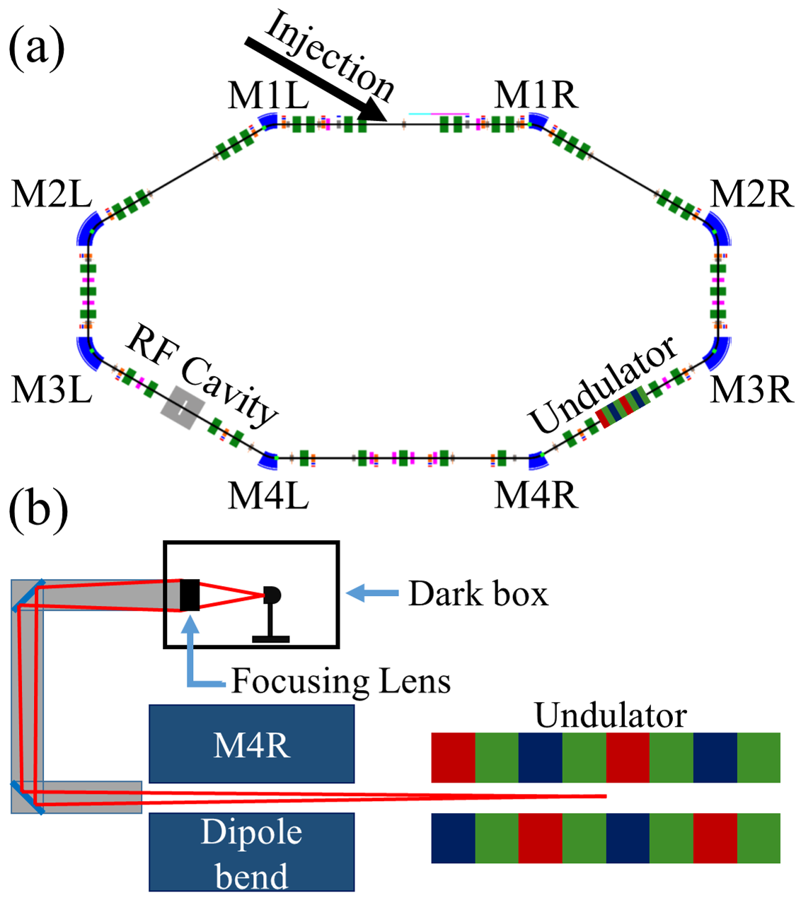
Figure 1: (a) Layout of IOTA. (b) Light path from the undulator to the detector (not to scale).

with a revolution period of $133.3\text{\,}\mathrm{n}\mathrm{s}$ and the beam energy of $$96.4\text{\,}$\pm$1\text{\,}\mathrm{M}\mathrm{e}\mathrm{V}$$. We studied two transverse focusing configurations in IOTA: (1) strongly coupled, resulting in approximately equal transverse mode emittances and (2) uncoupled, resulting in two drastically different emittances. Henceforth, we will refer to the beams in these configurations as “round” and “flat” beams, respectively. In both cases, the bunch length and the emittances depend on the beam current due to intra-beam scattering [32, 33], beam interaction with its environment [34], etc. The longitudinal bunch density distribution $\rho(z)$ was measured and recorded by a high-bandwidth wall-current monitor [35]. It was not exactly Gaussian, but this fact was properly accounted for by Eq. 6 for $\sigma_{z}^{\mathrm{eff}}$, which works for any longitudinal bunch shape. The IOTA rf cavity operated at $30\text{\,}\mathrm{M}\mathrm{H}\mathrm{z}$ (4th harmonic of the revolution frequency) with a voltage amplitude of about $360\text{\,}\mathrm{V}$. The rms momentum spread $\sigma_{p}$ was calculated from the known rf voltage amplitude, the design ring parameters and the measured rms bunch length $\sigma_{z}$. In our experiments, the relation was

$$\sigma_{p}\approx$9.1\text{\times}{10}^{-06}\text{\,}$\times\sigma_{z}[\mathrm{cm}].$$ (9)

It is an approximate equation, because of the bunch-induced rf voltage (beam loading) and a small deviation of $\rho(z)$ from the Gaussian shape. However, the effect of $\sigma_{p}$ in Eq. 2 in IOTA was almost negligible. Therefore, such estimation was acceptable.

For the round beam, the IOTA transverse focusing functions (4D Twiss functions) were chosen to produce approximately equal mode emittances at zero beam current, $\epsilon_{1}\approx\epsilon_{1}\approx$12\text{\,}\mathrm{n}\mathrm{m}$$ (rms, unnormalized). It was empirically confirmed that they remained equal at all beam currents with a few percent precision. The expected zero-current emittances for a flat beam were $\epsilon_{x}\approx$50\text{\,}\mathrm{n}\mathrm{m}$$, $\epsilon_{y}\gtrsim$0.33\text{\,}\mathrm{p}\mathrm{m}$$ (set by the quantum excitation in a perfectly uncoupled ring). The expected zero-current rms bunch length and the rms momentum spread for both round and flat beams were $\sigma_{z}=$9\text{\,}\mathrm{c}\mathrm{m}$$, $\sigma_{p}=$8.3\text{\times}{10}^{-05}\text{\,}$$. In our experiment, the electron beam sizes were monitored and recorded by visible synchrotron light image monitors (SLMs) [36] in seven dipole bend locations, at M1L-M4L and at M1R-M3R, see Fig. 1(a). The smallest reliably resolvable emittance by the SLMs in our experiment configuration was about $20\text{\,}\mathrm{n}\mathrm{m}$.

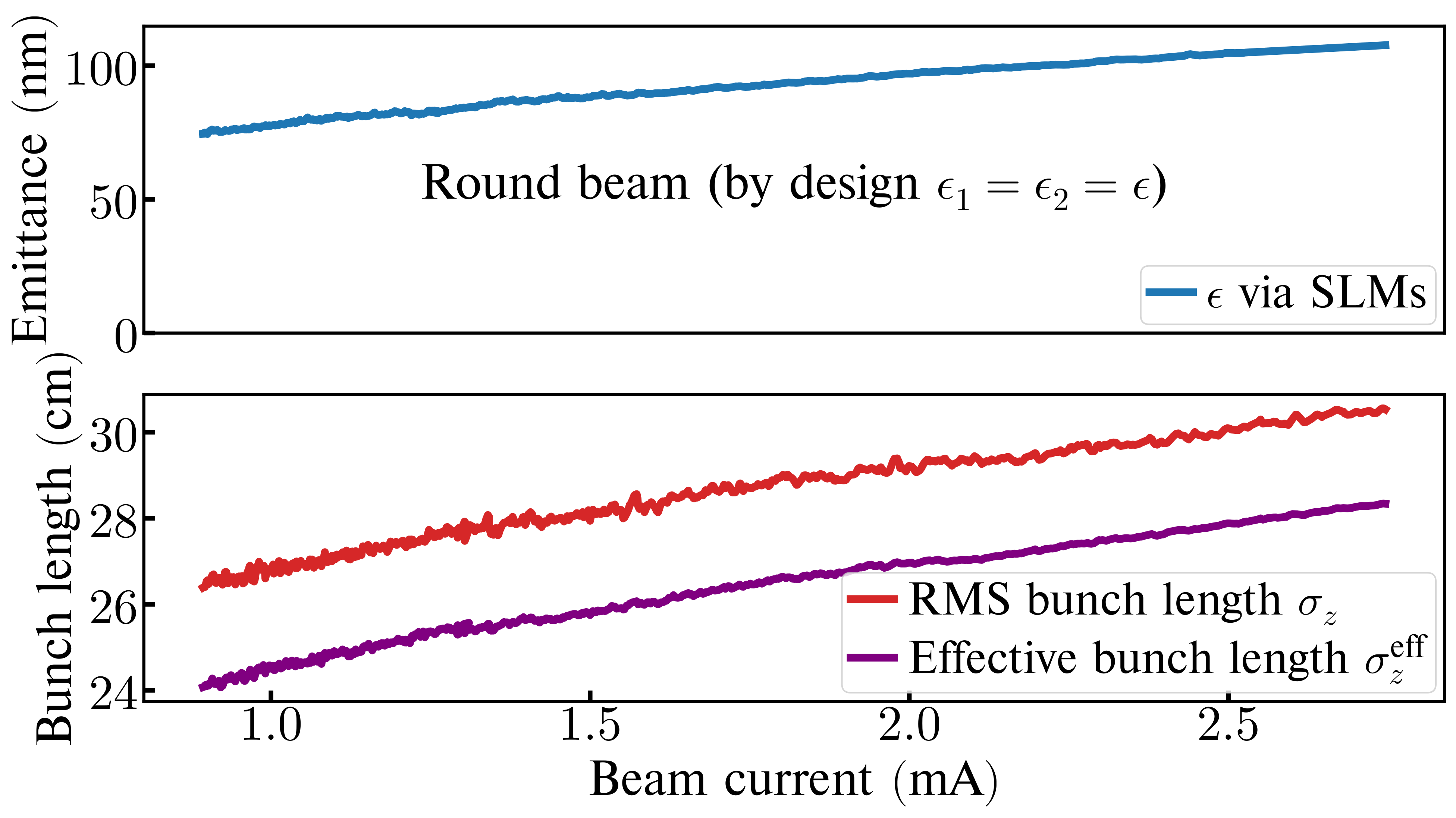
Figure 2: Mode emittances ($\epsilon_{1}=\epsilon_{2}=\epsilon$) and bunch lengths (rms and effective) of a round beam in IOTA as functions of beam current. SLMs had a monitor-to-monitor variation of $\pm$8\text{\,}\mathrm{n}\mathrm{m}$$ (not shown) in the measurement of $\epsilon$.

Figure 2 illustrates the bunch parameters of the round beam as a function of current. Below, we will present measurements with a flat beam at only one value of beam current, $2.66\text{\,}\mathrm{m}\mathrm{A}$, measured with a direct-current current transformer (DCCT). The parameters of the flat beam at this current value were $\sigma_{z}=$31.9\text{\,}\mathrm{c}\mathrm{m}$$, $\sigma_{z}^{\mathrm{eff}}=$29.5\text{\,}\mathrm{c}\mathrm{m}$$, $\sigma_{p}=$3.0\text{\times}{10}^{-04}\text{\,}$$. The horizontal emittance was $\epsilon_{x}=$0.66\text{\,}\mathrm{\SIUnitSymbolMicro}\mathrm{m}$$, as measured by the SLMs with a monitor-to-monitor variation of $\pm$50\text{\,}\mathrm{n}\mathrm{m}$$. The small vertical emittance of the flat beam was unresolvable by the SLMs. However, in Sec. V, we will demonstrate how it can be reconstructed using the fluctuations measurements.

At the center of the undulator, in the uncoupled optics, the Twiss parameters were $\beta_{x}=$204\text{\,}\mathrm{c}\mathrm{m}$$, $\beta_{y}=$98\text{\,}\mathrm{c}\mathrm{m}$$, $\alpha_{x}=$1.25\text{\,}$$, $\alpha_{y}=$-0.87\text{\,}$$, the horizontal dispersion $D_{x}=$101\text{\,}\mathrm{c}\mathrm{m}$$, its derivative $D_{x^{\prime}}=$-4.22\text{\,}$$. The strongly coupled optics was created from the uncoupled optics by changing the current in one skew-quad located at a zero dispersion location. The coupling parameter $u$ [37] was about $0.5\text{\,}$ everywhere in the ring. Therefore, the following is correct for the coupled case 4D Twiss functions, $\beta_{1x}\approx\beta_{2x}$, $\beta_{1y}\approx\beta_{2y}$. Moreover, their sums, $\beta_{1x}+\beta_{2x}$, $\beta_{1y}+\beta_{2y}$, were approximately equal to the Twiss beta functions in the uncoupled case, $\beta_{x}$, $\beta_{y}$. Equation (2) assumes an uncoupled optics. However, this specific strongly coupled optics used in IOTA can be approximated by the uncoupled optics with equal horizontal and vertical emittances $\epsilon_{x}=\epsilon_{y}=\epsilon$. More specifically, what is used in the derivation of Eq. 2 (see Appendix A) is the 6D phase-space distribution of the electrons, Eq. 34. This distribution, for the round beam, when calculated using the approximation of uncoupled optics with equal emittances $\epsilon_{x}=\epsilon_{y}=\epsilon$, and the distribution, calculated using the exact 4D Twiss functions and equal mode emittances, $\epsilon_{1}=\epsilon_{2}=\epsilon$, are almost indistinguishable. This property was intentionally included in the initial design of the coupled optics in IOTA.

The undulator strength parameter (peak) was $K_{\mathrm{u}}=$1.0\text{\,}$$ with the number of periods $N_{\mathrm{u}}=$10.5\text{\,}$$ and the period length $\lambda_{\mathrm{u}}=$5.5\text{\,}\mathrm{c}\mathrm{m}$$, the total length of the undulator was $L_{\mathrm{u}}=N_{\mathrm{u}}\lambda_{\mathrm{u}}=$58\text{\,}\mathrm{c}\mathrm{m}$$. A photodetector was installed in a dark box above the M4R dipole magnet, see Fig. 1(b). The light produced in the undulator was directed to the dark box by a system of two mirrors ($\diameter$2\text{\,}\mathrm{\text{\textquotedbl}}$$). Then, it was focused by a lens ($\diameter$2\text{\,}\mathrm{\text{\textquotedbl}}$$, focal distance $F=$150\text{\,}\mathrm{m}\mathrm{m}$$) into a spot, smaller than the sensitive area of the detector ($\diameter$1.0\text{\,}\mathrm{m}\mathrm{m}$$). The lens was $3.5\text{\,}\mathrm{m}$ away from the center of the undulator. Because of the two round mirrors, which are at $45\text{\,}\mathrm{\SIUnitSymbolDegree}$ to the direction of propagation of the radiation, the angular aperture takes an elliptical shape with the vertical axis smaller than the horizontal by a factor of $\sqrt{2}$. Namely, the horizontal and the vertical semi-axes were $7.3\text{\,}\mathrm{m}\mathrm{r}\mathrm{a}\mathrm{d}$ and $5.1\text{\,}\mathrm{m}\mathrm{r}\mathrm{a}\mathrm{d}$, respectively. The measurements were performed in the vicinity of the fundamental of the undulator radiation, $\lambda_{1}=\lambda_{\mathrm{u}}(1+K_{\mathrm{u}}^{2}/2)/(2\gamma^{2})=$1.16\text{\,}\mathrm{\SIUnitSymbolMicro}\mathrm{m}$$. As a photodetector we used an InGaAs PIN photodiode [38], which has a high quantum efficiency ($\approx$80\text{\,}\mathrm{\char 37\relax}$$) around the fundamental.

Using the elliptical angular aperture mentioned above and the manufacturers’ specifications for the spectral transmission of the vacuum chamber window at the M4R dipole magnet, the two mirrors, the focusing lens, and the quantum efficiency of the InGaAs photodiode, we constructed the detection efficiency function $\eta_{k,s}(\bm{\phi})$ for our system. The lens’s spectral transmission had to be linearly extrapolated for a small interval outside of the range provided in the manufacturer’s specifications. There were no free adjustable parameters. We calculated the field amplitude $\mathcal{E}_{k,s}(\bm{\phi})$, generated by a single electron, for the parameters of our undulator on a 3D grid ($k$, $\phi_{x}$, $\phi_{y}$) with our code [28]. Figure 3(a) shows the simulated spectrum, where the intensity is integrated over the elliptical aperture,

$$\derivative{\langle\mathcal{N}_{\mathrm{s.e.}}\rangle}{k}=\sum\limits_{s=1,2}\int\differential[2]{\bm{\phi}}\eta_{k,s}(\bm{\phi})\left|\mathcal{E}_{k,s}(\bm{\phi})\right|^{2}.$$ (10)

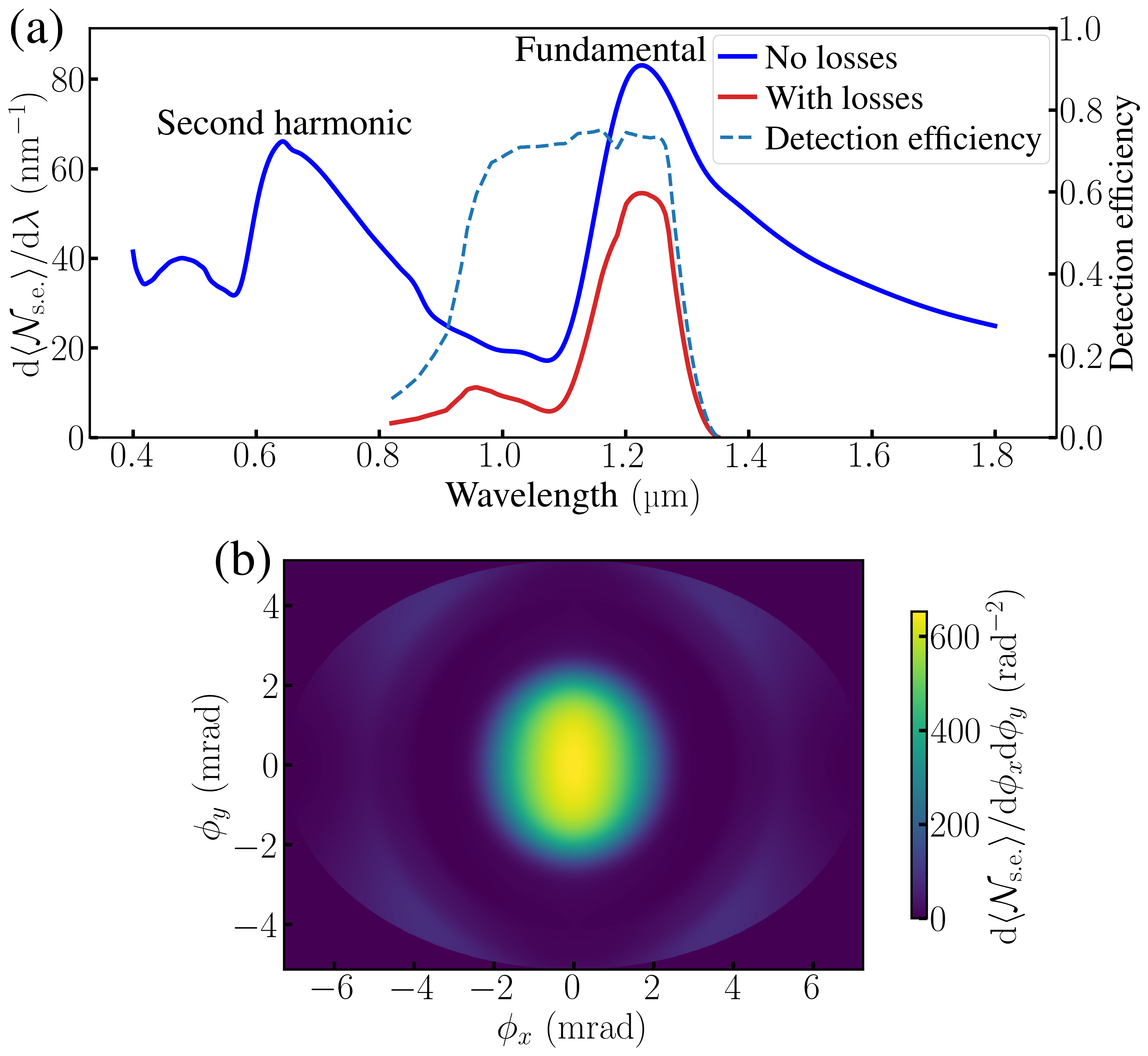
Figure 3: (a) Spectral distribution of the average number of detected photons per turn for a single electron (s.e.) assuming no losses (blue) and accounting for the detection efficiency of the system (red). Also, the detection efficiency (dashed, right vertical scale). (b) Angular distribution of the number of detected photons accounting for the detection efficiency of our system. Both (a) and (b) are calculated for an elliptical aperture with the horizontal and the vertical semi-axes $7.3\text{\,}\mathrm{m}\mathrm{r}\mathrm{a}\mathrm{d}$ and $5.1\text{\,}\mathrm{m}\mathrm{r}\mathrm{a}\mathrm{d}$, respectively.

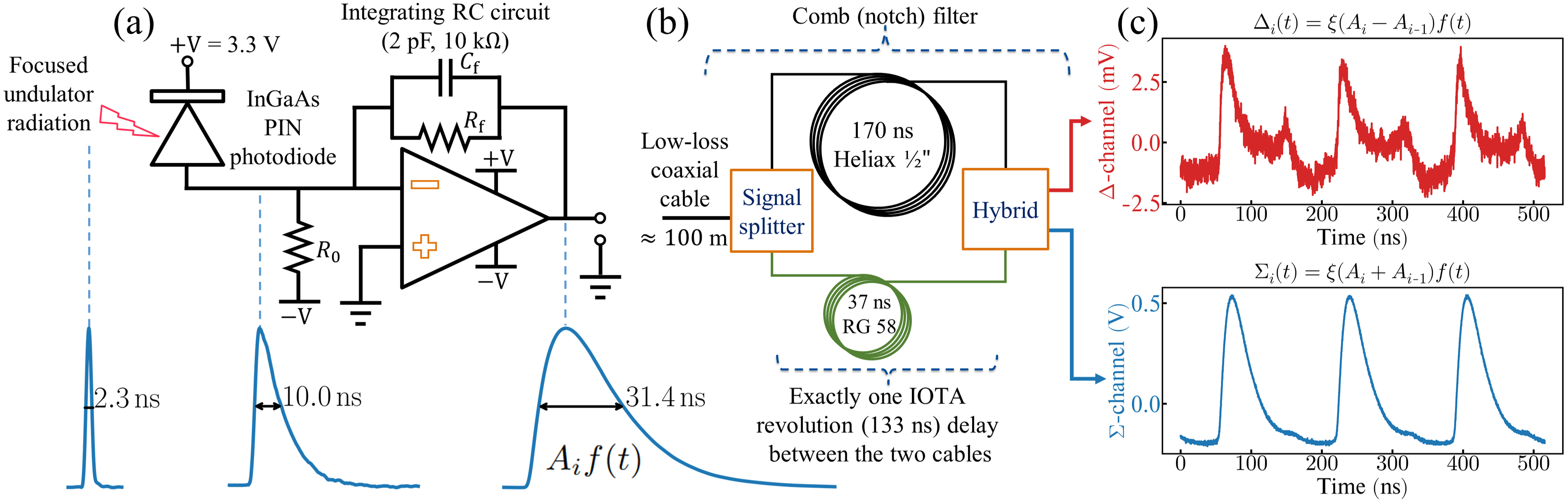
Figure 4: (a) Photocurrent integrator circuit. (b) Comb filter. (c) Sample waveforms of hybrid outputs ($\Delta$- and $\Sigma$-channels).

The blue line is calculated for an ideal detection system, where $\eta_{k,s}(\bm{\phi})=1$ inside the elliptical aperture, and zero outside. The red line is calculated with $\eta_{k,s}(\bm{\phi})$, constructed using the manufacturers’ specifications of the optical elements in our system. This $\eta_{k,s}(\bm{\phi})$ is equal to zero outside of the elliptical aperture. Whereas, inside, it is equal to the detection efficiency of our system. In our case, the detection efficiencies for the horizontal and vertical polarizations ($s=1,2$) are practically the same. Only the reflectance of the mirrors is slightly polarization dependent (under $1\text{\,}\mathrm{\char 37\relax}$ difference). Moreover, the radiation is dominated by the horizontal polarization (about $96.5\text{\,}\mathrm{\char 37\relax}$). The dashed line in Fig. 3(a) is the detection efficiency of our system for the horizontal polarization. Figure 3(b) shows the angular distribution with $\eta_{k,s}(\bm{\phi})$ of our system,

$$\frac{\differential[2]{\langle\mathcal{N}_{\mathrm{s.e.}}\rangle}}{\differential\phi_{x}\differential\phi_{y}}=\sum\limits_{s=1,2}\int\differential{k}\eta_{k,s}(\bm{\phi})\left|\mathcal{E}_{k,s}(\bm{\phi})\right|^{2}.$$ (11)

With the spectral properties of all optical elements in the system taken into account, the spectral width of the radiation was $0.14\text{\,}\mathrm{\SIUnitSymbolMicro}\mathrm{m}$ (FWHM), and the angular size was $\approx$2\text{\,}\mathrm{m}\mathrm{r}\mathrm{a}\mathrm{d}$$, which could be fully transmitted through the $\diameter$2\text{\,}\mathrm{\text{\textquotedbl}}$$ optical system.

Figure 4 illustrates our full photodetector circuit. First, the radiation pulse is converted into a photocurrent pulse by the photodiode, see Fig. 4(a). Then, the photocurrent pulse is integrated by an op-amp-based RC integrator, which outputs a longer pulse with a voltage amplitude that can be easily measured. The op-amp [39] was capable of driving the 50-$\Omega$ input load of a fast digitizing scope, located $\approx$100\text{\,}\mathrm{m}$$ away. The resistor $R_{0}=$580\text{\,}\mathrm{k\SIUnitSymbolOhm}$$ in the circuit in Fig. 4(a) was used to remove the offset in the integrator output signal (about $0.3\text{\,}\mathrm{V}$), produced by the op-amp input bias current and the photodiode leakage current. The output voltage pulse of the integrator at the $i$th IOTA turn can be represented as $A_{i}f(t)$, where $A_{i}$ is the signal amplitude at the $i$th turn and $f(t)$ is the average signal for one turn, normalized so that its maximum value is 1, see Fig. 4(a). The time $t$ in $f(t)$ is in the range $0133.3\text{\,}\mathrm{n}\mathrm{s}$, i.e., within one IOTA revolution. The number of photoelectrons, generated by the light pulse at the $i$th turn, $\mathcal{N}_{i}$, can be calculated as the time integral of the output pulse of the integrator divided by the electron charge $e$ and the resistance $R_{\mathrm{f}}$, i.e.,

$$\mathcal{N}_{i}=\int A_{i}f(t)\differential{t}/(eR_{\mathrm{f}}).$$ (12)

The function $f(t)$ is known — it was measured with a fast oscilloscope. It was practically the same during all of our measurements, because $f(t)$ is rather wide (about $30\text{\,}\mathrm{n}\mathrm{s}$ FWHM) and the length of the input light pulses was much smaller (about $2\text{\,}\mathrm{n}\mathrm{s}$ FWHM); moreover, the shape of input pulses did not change significantly. Therefore, during all of our measurements

$$\mathcal{N}_{i}=\chi A_{i},$$ (13)

where

$$\chi=\int f(t)\differential{t}/(eR_{\mathrm{f}})=$2.08\text{\times}{10}^{07}\text{\,}\mathrm{p}\mathrm{h}\mathrm{o}\mathrm{t}\mathrm{o}\mathrm{e}\mathrm{l}\mathrm{e}\mathrm{c}\mathrm{t}\mathrm{r}\mathrm{o}\mathrm{n}\mathrm{s}\mathrm{/}\mathrm{V}$,$$ (14)

with a $\pm$5\text{\,}\mathrm{\char 37\relax}$$ uncertainty, because of the uncertainty on $R_{\mathrm{f}}$. We verified Eq. 13 empirically at different voltage amplitudes $A_{i}$ and different bunch lengths, which define the lengths of the input light pulses. During our experiments at different beam currents, $A_{i}$ was in the range between $0\text{\,}\mathrm{V}$ and $1.2\text{\,}\mathrm{V}$.

Since we also knew the empirical linear relation between the beam current and the integrator voltage amplitude, we could use it in Eq. 13 to find the average number of detected photons (photoelectrons) per one electron of the electron bunch. The result of this calculation was $8.8\text{\times}{10}^{-03}\text{\,}\mathrm{p}\mathrm{h}\mathrm{o}\mathrm{t}\mathrm{o}\mathrm{e}\mathrm{l}\mathrm{e}\mathrm{c}\mathrm{t}\mathrm{r}\mathrm{o}\mathrm{n}\mathrm{s}\mathrm{/}\mathrm{e}\mathrm{l}\mathrm{e}\mathrm{c}\mathrm{t}\mathrm{r}\mathrm{o}\mathrm{n}$. This value is quite close to the result obtained in our simulation,

$$\sum\limits_{s=1,2}\int\differential{k}\differential[2]{\bm{\phi}}\eta_{k,s}(\bm{\phi})\left|\mathcal{E}_{k,s}(\bm{\phi})\right|^{2}\\ =$9.1\text{\times}{10}^{-03}\text{\,}\mathrm{p}\mathrm{h}\mathrm{o}\mathrm{t}\mathrm{o}\mathrm{e}\mathrm{l}\mathrm{e}\mathrm{c}\mathrm{t}\mathrm{r}\mathrm{o}\mathrm{n}\mathrm{s}\mathrm{/}\mathrm{e}\mathrm{l}\mathrm{e}\mathrm{c}\mathrm{t}\mathrm{r}\mathrm{o}\mathrm{n}$.$$ (15)

In our experiment, the expected relative fluctuation of $A_{i}$ was ${10}^{-4}\text{\,}$–${10}^{-3}\text{\,}$ (rms), which is considerably lower than the digitization resolution of our 8-bit broad-band oscilloscope. To overcome this problem, we used a passive comb (notch) filter [40], shown in Fig. 4(b). The signal splitter divides the integrator output into two identical signals. The lengths and the characteristics of the cables in the two arms were chosen such that one of the signals was delayed by exactly one IOTA revolution and, at the same time, the losses and dispersion in both arms were approximately equal. The time delay in the comb filter could be adjusted with a $0.1\text{\,}\mathrm{n}\mathrm{s}$ precision. Therefore, the time delay error was negligible, because the pulses at the entrance of the comb filter were about $30\text{\,}\mathrm{n}\mathrm{s}$ long (FWHM). Finally, a passive hybrid [41] generated the difference and the sum of the signals in the two arms — its output channels $\Delta$ and $\Sigma$, respectively. For an ideal comb filter,

$$\Delta_{i}(t)=\xi(A_{i}-A_{i\shortminus 1})f(t),$$ (16)

$$\Sigma_{i}(t)=\xi(A_{i}+A_{i\shortminus 1})f(t),$$ (17)

where we assume that the pulse shape of input and output signals of the comb filter is the same — $f(t)$. This means that we assume a negligible dispersion in the comb filter, which is a very good approximation according to our comparison of input and output pulses with the oscilloscope. Also, as a result of this comparison, we determined the parameter $\xi=$0.31\text{\,}$$. Of course, our comb filter was not perfect. There was some cross-talk between $\Delta$- and $\Sigma$-channels, some noise in the signals, a small undesirable reflection in one of the arms, resulting in a small satellite pulse about $85\text{\,}\mathrm{n}\mathrm{s}$ away from the main pulse, see Fig. 4(c). In addition, the hybrid was AC-coupled.

With these effects taken into account Eqs. 16 and 17 take the form

$$\Delta_{i}(t)=\xi(A_{i}-A_{i\shortminus 1})f(t)+\mu_{\Delta}\Sigma_{i}(t)\\ +\delta_{r}A_{i}f(t-t_{r})+\nu_{\Delta_{i}}(t)-\Delta_{\mathrm{AC}},$$ (18)

$$\Sigma_{i}(t)=\xi(A_{i}+A_{i\shortminus 1})f(t)+\mu_{\Sigma}\Delta_{i}(t)\\ +\delta_{r}A_{i}f(t-t_{r})+\nu_{\Sigma_{i}}(t)-\Sigma_{\mathrm{AC}},$$ (19)

where $t$ is within one IOTA turn ($0133.3\text{\,}\mathrm{n}\mathrm{s}$), $\mu_{\Delta}$ and $\mu_{\Sigma}$ describe the cross-talk between $\Delta$- and $\Sigma$-channels ($<$1\text{\,}\mathrm{\char 37\relax}$$), $\delta_{r}A_{i}f(t-t_{r})$ describes the reflected pulse in one of the arms (perhaps the short one), $t_{r}=$85\text{\,}\mathrm{n}\mathrm{s}$$, $\delta_{r}\approx$1.5\text{\times}{10}^{-3}\text{\,}$$; and it is assumed that the noise contributions $\nu_{\Delta_{i}}(t)$ and $\nu_{\Sigma_{i}}(t)$ enter the equations as sum terms, independent of the signal amplitude; the constants $\Delta_{\mathrm{AC}}$ and $\Sigma_{\mathrm{AC}}$ come from the fact that the hybrid is AC-coupled and the averages of $\Delta_{i}(t)$ and $\Sigma_{i}(t)$ over a long time have to be zero.

For each measurement, we recorded $1.5\text{\,}\mathrm{m}\mathrm{s}$-long waveforms (about $n_{\mathrm{rev}}=$11\,250\text{\,}$$ IOTA revolutions) of $\Delta$- and $\Sigma$-channels with the oscilloscope at $20\text{\,}\mathrm{G}\mathrm{S}\mathrm{a}\mathrm{/}\mathrm{s}$. The beam current decay was negligible during this $1.5\text{\,}\mathrm{m}\mathrm{s}$ acquisition period.

In Eq. 19, the noise, the cross-talk term, and the reflection term are negligible. The $\Sigma$-channel can be used to measure the photoelectron count mean $\langle\mathcal{N}\rangle$ during the $1.5\text{\,}\mathrm{m}\mathrm{s}$. Using Eq. 13 and the non-negligible part of Eq. 19,

$$\langle\mathcal{N}\rangle=\chi\frac{\langle\Sigma(t_{\mathrm{peak}})\rangle+\Sigma_{\mathrm{AC}}}{2\xi},$$ (20)

where we introduced $t_{\mathrm{peak}}$ — the time within each turn, corresponding to the peak of the signal, $f(t_{\mathrm{peak}})=1$,

$$\langle\Sigma(t_{\mathrm{peak}})\rangle=\frac{1}{n_{\mathrm{rev}}}\sum\limits_{i=1}^{n_{\mathrm{rev}}}\Sigma_{i}(t_{\mathrm{peak}}).$$ (21)

The idea of using a comb filter is that, in the ideal case, see Eq. 16, the $\Delta$-channel would provide the exact difference between two consecutive turns in IOTA. In this case we would be able to look directly at the turn-to-turn fluctuations. The offset would be removed, and the oscilloscope could be used with the appropriate scale setting, with negligible digitization noise. In our non-ideal comb filter, see Eq. 18, the additional terms have some impact on the $\Delta$-signal, see Fig. 4(c). Nonetheless, by analyzing the $\Delta$-signal in a special way, described below, it is possible to determine $\mathrm{var}(\mathcal{N})$ with sufficient precision.

Namely, if we take the variance of Eq. 18 with respect to $i$ at a fixed time $t$, then we obtain

$$\mathrm{var}(\Delta(t))=2\xi^{2}\mathrm{var}(A)f^{2}(t)+\mathrm{var}(\nu_{\Delta}(t)),$$ (22)

where the contribution from $\mu_{\Delta}\Sigma_{i}(t)$ and $\delta_{r}A_{i}f(t)$ may be dropped, because the fluctuations of $\Sigma_{i}(t)$ and $A_{i}$ are strongly attenuated by the factors $\mu_{\Delta}$ and $\delta_{r}$, respectively. Also, $\mathrm{var}(\Delta_{\mathrm{AC}})=0$ since $\Delta_{\mathrm{AC}}$ is constant during the $1.5\text{\,}\mathrm{m}\mathrm{s}$. The left-hand side of Eq. 22, as a function of $t\in[0,$133.3\text{\,}$]$\text{\,}\mathrm{n}\mathrm{s}$$, could be obtained from the collected waveforms of $\Delta$-channel as

$$\mathrm{var}(\Delta(t))=\frac{1}{n_{\mathrm{rev}}}\sum\limits_{i=1}^{n_{\mathrm{rev}}}\Delta_{i}^{2}(t)-\bigl{[}\frac{1}{n_{\mathrm{rev}}}\sum\limits_{i=1}^{n_{\mathrm{rev}}}\Delta_{i}(t)\bigr{]}^{2}.$$ (23)

The results of such calculation for 2000 moments of time $t$ within an IOTA revolution are shown in Fig. 5. These data are for the round beam. The blue, orange, and green lines correspond to three significantly different values of beam current within the range studied in our experiment; the red line corresponds to a zero beam current case.

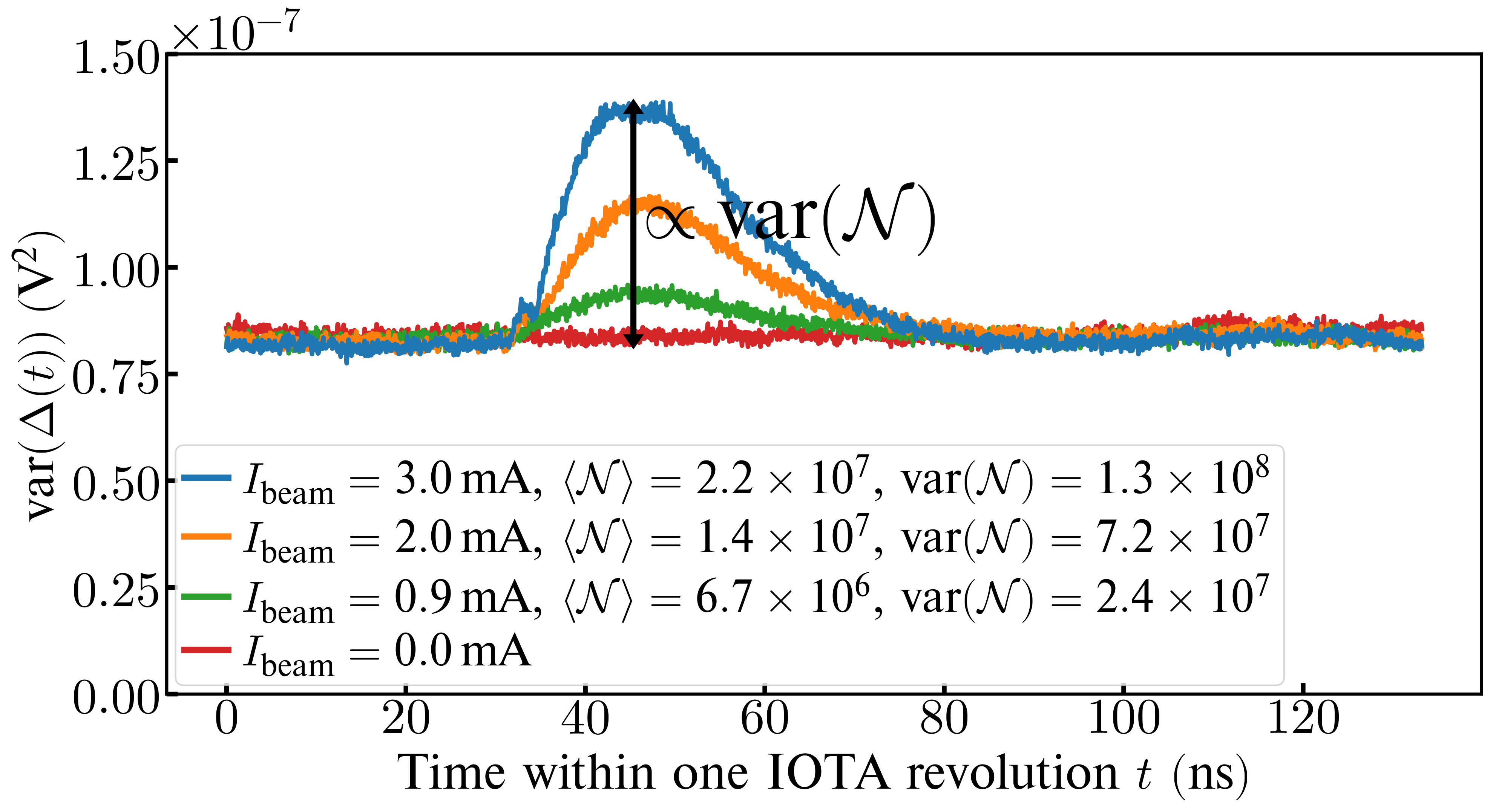
Figure 5: The variance of $\Delta$-signal as a function of time (see Eq. 22) within one IOTA revolution (round-beam data).

Figure 5 suggests that there is a constant noise level, independent of time and independent of the signal amplitude. Specifically, it suggests that the noise term in Eq. 22 is

$$\mathrm{var}(\nu_{\Delta}(t))=\mathrm{var}(\nu_{\Delta})=$8.8\text{\times}{10}^{-8}\text{\,}\mathrm{V}$^{2}.$$ (24)

The observed rms noise amplitude ($\approx$0.3\text{\,}\mathrm{m}\mathrm{V}$$) was analyzed by using the noise model for the detector electrical schematic, Figs. 4(a) and (b), as well as the typical electrical characteristics of the photodiode [38] and the operational amplifier [39]. The three main contributions to the rms noise in the $\Delta$-channel are the following: the oscilloscope input amplifier noise, $0.21\text{\,}\mathrm{m}\mathrm{V}$; the operational amplifier input voltage noise, $0.18\text{\,}\mathrm{m}\mathrm{V}$; and the operational amplifier input current noise, $0.037\text{\,}\mathrm{m}\mathrm{V}$. When added in quadrature, these three sources explain the measured noise level.

The peaks rising above the noise level in Fig. 5 can be fitted well with $f^{2}(t)$ (fits not shown). Thus, their shape is in agreement with Eq. 22 as well.

Therefore, using Eqs. 13 and 22, the photoelectron count variance $\mathrm{var}(\mathcal{N})$ can be determined as

$$\mathrm{var}(\mathcal{N})=\chi^{2}\mathrm{var}(A)=\chi^{2}\frac{\mathrm{var}(\Delta(t_{\mathrm{peak}}))-\mathrm{var}(\nu_{\Delta})}{2\xi^{2}},$$ (25)

see Eq. 23 for the definition of $\mathrm{var}(\Delta(t_{\mathrm{peak}}))$. The value of the noise level term in Eq. 25 is

$$\frac{\chi^{2}\mathrm{var}(\nu_{\Delta})}{2\xi^{2}}=$2.0\text{\times}{10}^{08}\text{\,}$.$$ (26)

We employed a dedicated test light source with known fluctuations to verify this method of measurement of $\langle\mathcal{N}\rangle$ and $\mathrm{var}(\mathcal{N})$ [Eqs. 20 and 25]. This verification is described in Appendix C, where we also estimated the statistical error of the measurement of $\mathrm{var}(\mathcal{N})$ by our apparatus, namely, $\pm$2.7\text{\times}{10}^{06}\text{\,}$$ — it is approximately constant in the range of $\mathrm{var}(\mathcal{N})$ observed with the undulator radiation in IOTA.

IV Measurement results

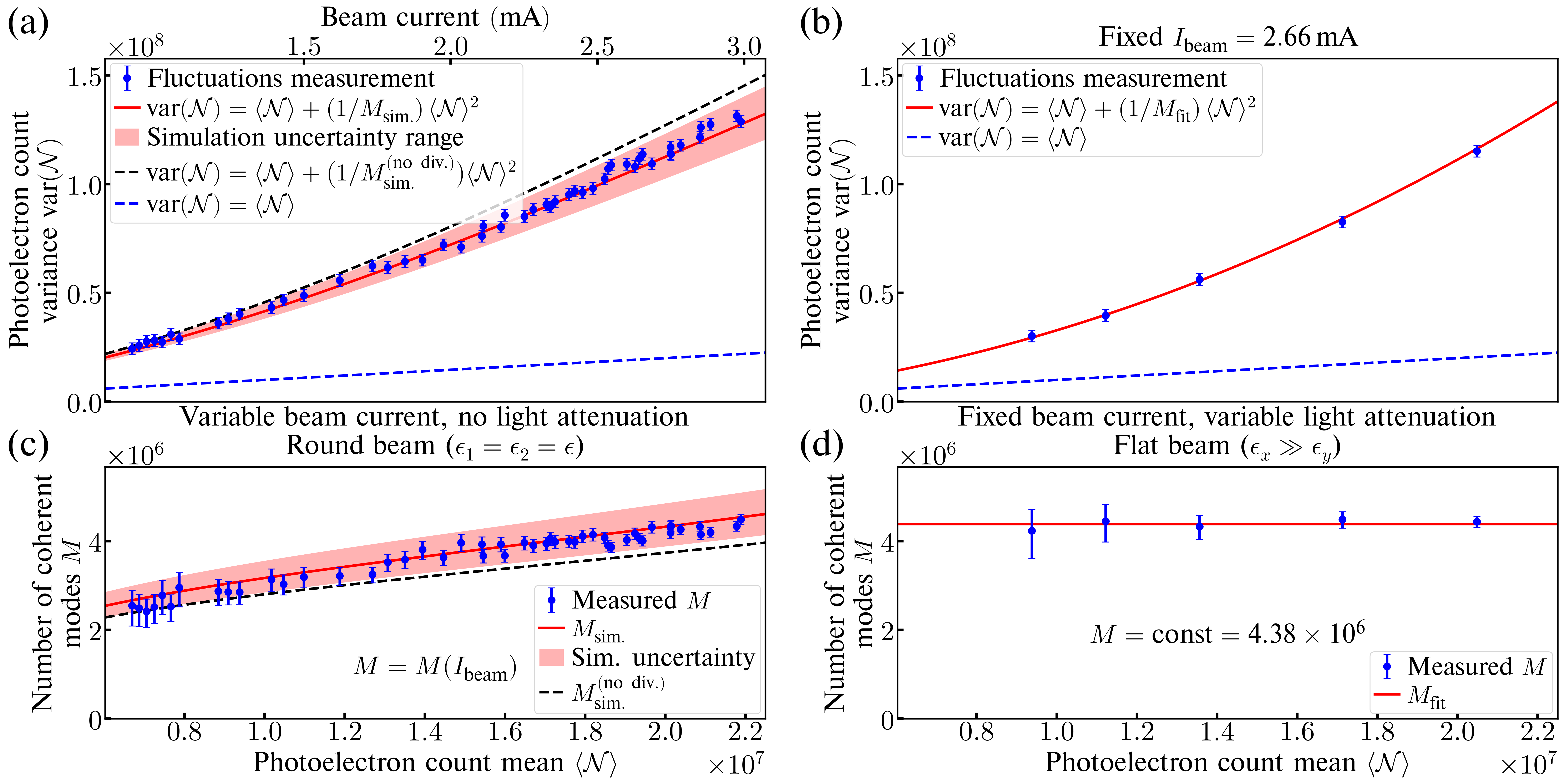
Figure 6: (a) The fluctuations measurement for the round electron beam in IOTA as a function of beam current, a prediction by Eq. 2 (red solid line) and a prediction by [5, Eq. (49)] (black dashed line), which does not account for the beam divergence. (b) The fluctuations measurement for the flat electron beam at a fixed beam current $2.66\text{\,}\mathrm{m}\mathrm{A}$ with 4 different optical neutral density filters and one point without any filters, as well as a parabolic fit (a prediction could not be made, because the vertical emittance of the flat beam was unknown). (c) and (d) present the data of (a) and (b) in terms of the number of coherent modes $M$.

The measured fluctuations data for the round beam at different values of beam current are shown in Fig. 6(a) (blue points). The blue dashed straight line, $\mathrm{var}(\mathcal{N})=\langle\mathcal{N}\rangle$, represents the photon shot noise contribution to the fluctuations — the first sum term in Eq. 1. The values of $M$ extracted from the fluctuation data points using the equation,

$$M=\langle\mathcal{N}\rangle^{2}/(\mathrm{var}(\mathcal{N})-\langle\mathcal{N}\rangle),$$ (27)

are shown in Fig. 6(c) (blue points). The error bars in Figs. 6(a),(c) correspond to the $\pm$2.7\text{\times}{10}^{06}\text{\,}$$ statistical error of measurement of $\mathrm{var}(\mathcal{N})$ by our technique. Further, Fig. 6(c) has a curve for $M$, simulated by Eq. 2 (red line), and, for comparison, a curve for $M$, simulated by [5, Eq. (49)] (dashed black line), which neglects beam divergence. Corresponding curves for simulated $\mathrm{var}(\mathcal{N})$ are shown in Fig. 6(a). The shaded light red areas in Figs. 6(a),(c) show the uncertainty range of our simulation by Eq. 2.

For this simulation, we needed the values of the following four bunch parameters, entering Eq. 2, $\epsilon_{x}$, $\epsilon_{y}$, $\sigma_{p}$, $\sigma_{z}^{\mathrm{eff}}$, at all beam currents. Further, we needed the values of Twiss functions in the undulator, the parameters of the undulator and of the detection system. All these aspects were described in Sec. III. We had no free parameters in this simulation. Numerical calculation of the integrals in Eq. 2 and [5, Eq. (49)] was performed by the Monte-Carlo algorithm on the Midway2 cluster at the University of Chicago Research Computing Center using our computer code [31, 28].

The simulation uncertainty range (shaded light red area) primarily comes from the uncertainty in the beam energy $$96.4\text{\,}$\pm$1\text{\,}\mathrm{M}\mathrm{e}\mathrm{V}$$. The next source of uncertainty by magnitude, which is a factor of two smaller, is the SLMs’ $\pm$8\text{\,}\mathrm{n}\mathrm{m}$$ monitor-to-monitor variation of $\epsilon$ [for the round beam we use $\epsilon_{x}=\epsilon$ and $\epsilon_{y}=\epsilon$ in Eq. 2]. The uncertainties of other parameters ($\sigma_{p}$, $\sigma_{z}^{\mathrm{eff}}$, Twiss functions in the undulator, etc.) had negligible effect. The manufacturers’ specifications for the optical elements of our system did not provide any uncertainties. Therefore, they were not considered.

We also collected fluctuations data for another experiment configuration. Figure 6(b) shows fluctuation data points for a flat beam (uncoupled focusing) at a fixed beam current $2.66\text{\,}\mathrm{m}\mathrm{A}$. The corresponding reconstructed values of $M$ are shown in Fig. 6(d). The error bars in Figs. 6(b),(d) correspond to the $\pm$2.7\text{\times}{10}^{06}\text{\,}$$ statistical error of measured $\mathrm{var}(\mathcal{N})$. In this measurement, the photoelectron count mean (horizontal axis) was varied by using different optical neutral density filters (one point without a filter and four points with filters). Neutral density filters are filters that have constant attenuation in a certain wavelength range; in our case, around the fundamental harmonic of the undulator radiation. A new bunch was injected into the ring for each measurement. The oscilloscope waveforms for $\Delta$- and $\Sigma$-channels were recorded when the beam current decayed to $2.66\text{\,}\mathrm{m}\mathrm{A}$. The red curve in Fig. 6(b) is a fit with a constant $M$. A corresponding horizontal line is shown in Fig. 6(d). The value of $M$ in this fit is $M_{\mathrm{fit}}=(4.38\pm 0.10)\times 10^{6}$. This value was calculated as the average of the five values of $M$ in Fig. 6(d), and the error was calculated as the standard deviation of these five values.

We do not present any simulation results for the fluctuations $\mathrm{var}(\mathcal{N})$ in the uncoupled focusing, because the SLMs provided very inconsistent estimates for the small vertical emittance $\epsilon_{y}$ of the flat beam — the max-to-min variation for different SLMs reached a factor of eight. We believe this happened because the beam images were close to the resolution limit, set by a combination of factors, such as the diffraction limit, the point spread function of the cameras, chromatic aberrations, the effective radiator size of the dipole magnet radiation ($\approx$20\text{\,}\mathrm{\SIUnitSymbolMicro}\mathrm{m}$$), and the camera pixel size ($\approx$10\text{\,}\mathrm{\SIUnitSymbolMicro}\mathrm{m}$$ in terms of beam size). Therefore, the monitor-to-monitor emittance value variation primarily came from the Twiss beta-function variation ($\beta_{y}^{(\mathrm{max})}/\beta_{y}^{(\mathrm{min})}\approx 12$). The diffraction limit is primarily caused by the irises, used to reduce the radiation intensity to prevent the cameras from saturating at high beam currents. Alternatively, leaving the irises open and using attenuating optical filters may improve the resolution. Additional negative effects include the errors in the light focusing optics, calibration errors of the SLMs, and possible Twiss beta-function errors. The SLMs at locations with larger beta-functions (M4L, M1L) provide estimates for $\epsilon_{y}$ that agree better with the theoretical predictions [42] at lower beam currents, and with the emittance estimates presented below in this paper. Nevertheless, we cannot state that the SLMs could provide a reliable estimate for $\epsilon_{y}$ during our experiment.

Without $\epsilon_{y}$ we could not use Eq. 2 to make a prediction for $M$ and $\mathrm{var}(\mathcal{N})$. However, we attempted the reverse of this procedure, namely, the reconstruction of the unknown $\epsilon_{y}$ via the measured fluctuations for the flat beam shown in Figs. 6(b),(d). Indeed, the measured value of the number of coherent modes $M_{\mathrm{meas}}$ is a function of four bunch parameters,

$$M_{\mathrm{meas}}=M(\epsilon_{x},\epsilon_{y},\sigma_{p},\sigma_{z}^{\mathrm{eff}}).$$ (28)

The full form of the right-hand side is given by Eq. 2. The horizontal emittance $\epsilon_{x}$ of the flat beam at a beam current of $2.66\text{\,}\mathrm{m}\mathrm{A}$ could still be reliably measured via the SLMs, yielding $\epsilon_{x}=$0.66\text{\,}\mathrm{\SIUnitSymbolMicro}\mathrm{m}$$. The effective bunch length $\sigma_{z}^{\mathrm{eff}}$ could be determined from $\rho(z)$ measured by the wall-current monitor, $\sigma_{z}^{\mathrm{eff}}=$29.5\text{\,}\mathrm{c}\mathrm{m}$$. The rms momentum spread $\sigma_{p}$ was estimated from $\rho(z)$ and the ring parameters, $\sigma_{p}=$3.0\text{\times}{10}^{-04}\text{\,}$$. The only unknown in Eq. 28 is $\epsilon_{y}$. Equation (28) can be solved for $\epsilon_{y}$ by a simple bisection method. The result is $\epsilon_{y}=$8.4\text{\,}$\pm$1.5\text{\,}\mathrm{n}\mathrm{m}$$, where the uncertainty corresponds to the statistical error of $M_{\mathrm{fit}}$, mentioned above. For comparison, we also used [5, Eq. (49)]  in Eq. 28, which neglects beam divergence. In this case, we obtained $\epsilon_{y}=$18.3\text{\,}$\pm$1.3\text{\,}\mathrm{n}\mathrm{m}$$.

In this reconstruction of $\epsilon_{y}$, there is also a systematic error due to the uncertainty on the beam energy ($\pm$1\text{\,}\mathrm{M}\mathrm{e}\mathrm{V}$$) and due to the systematic error of $\epsilon_{x}$ measurement by the SLMs ($\pm$50\text{\,}\mathrm{n}\mathrm{m}$$ monitor-to-monitor). We estimated these two contributions to the systematic error of $\epsilon_{y}$ from Eq. 2. They are $\begin{subarray}{c}+2.5\\ -4.5\end{subarray}\;$\text{\,}\mathrm{n}\mathrm{m}$$ and $\begin{subarray}{c}+1.6\\ -1.4\end{subarray}\;$\text{\,}\mathrm{n}\mathrm{m}$$, respectively. These systematic errors are rather significant. However, they are not directly linked to our measurement technique. They are related to the fact that the beam energy and the horizontal emittance of a flat beam in IOTA were not known with better precision. Further improvements in beam characterization in IOTA will reduce the systematic error of our fluctuations-based technique of $\epsilon_{y}$ measurement.

V Discussion and conclusions

Power fluctuations in undulator radiation were measured in IOTA under two different experimental conditions and compared with our theoretical predictions.

The fluctuations predicted by Eqs. 1 and 2 in the round beam configuration agree with the measurements within the uncertainties, as shown in Figs. 6(a),(c). In IOTA, the bunch parameters $\epsilon_{x}$, $\epsilon_{y}$, $\sigma_{p}$, $\sigma_{z}^{\mathrm{eff}}$ depend on the beam current because of various intensity dependent effects, e.g., intra-beam scattering [43], beam interaction with its environment [34], etc. Therefore, $M$ is a function of the beam current as well, as one can see in Fig. 6(c).

In Figs. 6(b),(d), all data points correspond to one value of the beam current, $2.66\text{\,}\mathrm{m}\mathrm{A}$. The photoelectron count mean is varied by using neutral density filters with different attenuation factors $\eta_{\mathrm{ND}}$. Such filters linearly scale down the photoelectron count mean, $\langle\mathcal{N}\rangle\rightarrow\eta_{\mathrm{ND}}\langle\mathcal{N}\rangle$. However, they do not change $M$, because if $\eta_{k,s}(\bm{\phi})$ is replaced by $\eta_{\mathrm{ND}}\eta_{k,s}(\bm{\phi})$ in Eq. 2, then $\eta_{\mathrm{ND}}$ cancels out in the numerator and the denominator. This is consistent with Fig. 6(d) — all measured values of $M$ are equal within the uncertainty range.

We reconstructed the value of the vertical emittance $\epsilon_{y}$ of the flat beam from $M_{\mathrm{fit}}$ via Eq. 2 and via [5, Eq. (49)], which neglects beam divergence. We obtained very different results, $\epsilon_{y}=$8.4\text{\,}$\pm$1.5\text{\,}\mathrm{n}\mathrm{m}$$ and $\epsilon_{y}=$18.3\text{\,}$\pm$1.3\text{\,}\mathrm{n}\mathrm{m}$$, respectively. This shows that, for the flat beam, accounting for the beam divergence is critical. In this measurement, the horizontal beam divergence was $0.94\text{\,}\mathrm{m}\mathrm{r}\mathrm{a}\mathrm{d}$ and comparable with the rms radiation divergence $\sqrt{\lambda_{1}/(2L_{\mathrm{u}})}=$1.0\text{\,}\mathrm{m}\mathrm{r}\mathrm{a}\mathrm{d}$$ [1, Eq. (2.57)], which gives an estimate of the angular size of $\mathcal{E}_{k,s}(\bm{\phi})$. Clearly, in this case it has a significant effect on the integral in the numerator of Eq. 2. This is why we use Eq. 2 in our Letter [24], focused on emittance measurements via fluctuations, as opposed to [5, Eq. (49)], which is simpler, but neglects beam divergence.

In addition, we made an independent estimate of the vertical emittance $\epsilon_{y}$ of the flat beam based on the beam lifetime, see Appendix D for details. At the beam current of $2.66\text{\,}\mathrm{m}\mathrm{A}$, the beam lifetime is solely determined by Touschek scattering [42, 37, 44]. The Touschek lifetime is a function of beam emittances and bunch length. Therefore, since we knew the horizontal emittance $\epsilon_{x}$ of the flat beam, measured by the SLMs, the bunch length, measured by the wall-current monitor, and the measured beam lifetime $\left|I/(\derivative*{I}{t})\right|$, we could find $\epsilon_{y}$. The result is $\epsilon_{y}=$9.6\text{\,}$\pm$1.2\text{\,}\mathrm{n}\mathrm{m}$$, to be compared with the fluctuations-based measurement, $\epsilon_{y}=$8.4\text{\,}$\pm$1.5\text{\,}\mathrm{n}\mathrm{m}$$. The $\pm$1.2\text{\,}\mathrm{n}\mathrm{m}$$ error in the lifetime-based $\epsilon_{y}$ estimate comes from the $\pm$50\text{\,}\mathrm{n}\mathrm{m}$$ uncertainty on $\epsilon_{x}$ of the flat beam.

In the round beam case, at the same beam current of $2.66\text{\,}\mathrm{m}\mathrm{A}$, the beam divergence in the undulator was about $0.43\text{\,}\mathrm{m}\mathrm{r}\mathrm{a}\mathrm{d}$ (both $x$ and $y$). It was noticeably smaller than the horizontal beam divergence of the flat beam and than the rms radiation divergence $1.0\text{\,}\mathrm{m}\mathrm{r}\mathrm{a}\mathrm{d}$. Therefore, the effect of beam divergence on the fluctuations simulation in Figs. 6(a),(c) is not as dramatic. However, the deviation from the measurement of the simulation based on [5, Eq. (49)], which neglects beam divergence, is certainly noticeable, whereas the simulation by Eq. 2 agrees well with the measurement.

It would be beneficial to repeat these fluctuation measurements with a longer and brighter undulator. In this experiment, we had to avoid using a monochromator or restricting the angular aperture, because we had to collect all available radiation to achieve a signal with a voltage amplitude that could be easily measured. Therefore, the integrals in Eqs. 2 and 5 had to be calculated over a broad range of angles and wavelengths. With a monochromator, a slit or a pinhole detector, these integrals could be significantly simplified. Further, if our undulator had more periods and if we were able to use a monochromator, we could slowly vary the beam energy and find the energy at which the detected power is at maximum, i.e., when we are centered on the peak of the fundamental harmonic. In this case, the systematic error of the $\epsilon_{y}$ measurement via the fluctuations, related to the uncertainty on the beam energy, would be negligible. Moreover, it can be shown [24] that if one places a narrow vertical slit in front of the detector, then the magnitude of the fluctuations would only depend on $\epsilon_{y}$, i.e., the systematic error of the $\epsilon_{y}$ measurement related to the uncertainty of $\epsilon_{x}$, measured by the SLMs, would be minimized, too. Finally, for a brighter undulator, the statistical error on the measured value of the fluctuations would be lower as well.

We are considering using our fluctuations measurement apparatus, or an improved variation of it, as a tool for the diagnostics of the Optical Stochastic Cooling (OSC) experiment in IOTA [45, 46, 47]. In this experiment, the beam emittance will be even smaller and the existing diagnostic tools may not have sufficient resolution. Even though we cannot measure transverse emittances and bunch lengths individually in this way, the fluctuations may serve as an indicator of the cooling process. When the cooling process starts, the electron bunch shrinks, which, in turn, makes the fluctuations of the number of detected photons increase.

To conclude, we presented a calculation [Eqs. 1 and 2], which describes the turn-to-turn fluctuations in the number of detected synchrotron radiation photons, produced by an electron bunch with a Gaussian transverse density distribution, an arbitrary longitudinal density distribution, and non-negligible rms beam divergences. The rms bunch length is assumed to be significantly larger than the radiation wavelength. Equation (2) is presented for the first time, as beam divergence has been neglected in all previous considerations [6, 5]. Beam divergence can be neglected if it is significantly smaller than the characteristic radiation angle — $\sqrt{\lambda_{1}/(2L_{\mathrm{u}})}$ for the fundamental of undulator radiation. We presented the results of an experiment with a round beam in IOTA, where beam divergence had an impact on the fluctuations of the undulator radiation. We showed that our new Eq. 2 agrees better with the measurements than [5, Eq. (49)], which neglects beam divergence. Finally, we proposed a non-invasive technique to measure the small unknown vertical emittance of a flat beam via the fluctuations. This new technique is described in detail in a separate publication [24].

Appendix A Derivation of the fluctuations with a considerable beam divergence

Previously, we derived an equation for $M$ [5, Eq. (49)] for the case of a monoenergetic beam, zero beam divergence and temporally incoherent radiation. Below we outline the steps to extend this result to the case of a considerable beam divergence [see Eq. 2].

One can start from [5, Eq. (21)], but written in a form that accounts for the beam divergence, namely,

$$\mathrm{var}(\mathcal{N})=\langle\mathcal{N}\rangle-\langle\mathcal{N}\rangle^{2}\\ +\int\differential{\xi}\,p(\xi)\Bigl{[}\sum\limits_{s=1,2}\int\differential{k}\differential[2]{\bm{\phi}}\eta_{k,s}(\bm{\phi})\bigl{|}\sum\limits_{m}\mathcal{E}_{k,s}^{(m)}(\bm{\phi})\bigr{|}^{2}\Bigr{]}^{2},$$ (29)

where $\xi$ describes the states in the 6D phase-space of all the electrons in the center of the radiator,

$$\xi=\tilde{x}_{1},\tilde{x}^{\prime}_{1},y_{1},y^{\prime}_{1},t_{1},\delta p_{1}\\ \dots\tilde{x}_{n_{e}},\tilde{x}^{\prime}_{n_{e}},y_{n_{e}},y^{\prime}_{n_{e}},t_{n_{e}},\delta p_{n_{e}},$$ (30)

where $t_{m}$ is the time when the $m$th electron passes the center of the synchrotron light source, $\,p(\xi)$ represents the density function for the probability to have the state $\xi$,

$$\,p(\xi)=p(\tilde{x}_{1},\tilde{x}^{\prime}_{1},y_{1},y^{\prime}_{1},t_{1},\delta p_{1})\\ \dots p(\tilde{x}_{n_{e}},\tilde{x}^{\prime}_{n_{e}},y_{n_{e}},y^{\prime}_{n_{e}},t_{n_{e}},\delta p_{n_{e}}),$$ (31)

$\tilde{x}_{m}$ and $\tilde{x}^{\prime}_{m}$ refer to the monoenergetic component of the motion, because there is also a contribution from the horizontal dispersion, so that

$$x_{m}=\tilde{x}_{m}+D_{x}\delta p_{m}, x^{\prime}_{m}=\tilde{x}^{\prime}_{m}+D_{x^{\prime}}\delta p_{m},$$ (32)

and the vertical dispersion is assumed to be zero. According to [1, Eq. (2.93)], the complex field amplitude of the $m$th electron $\mathcal{E}_{k,s}^{(m)}(\bm{\phi})$ can be expressed through the amplitude of the reference electron $\mathcal{E}_{k,s}(\bm{\phi})$ [see Eq. 7] as

$$\mathcal{E}_{k,s}^{(m)}(\bm{\phi})=e^{ict_{m}-ik_{x}x_{m}-ik_{y}y_{m}}\mathcal{E}_{k,s}(\bm{\phi}-\bm{r}^{\prime}_{m}),$$ (33)

where $\bm{r}^{\prime}_{m}=(x^{\prime}_{m},y^{\prime}_{m})$ and it is assumed that $\mathcal{E}_{k,s}^{(m)}(\bm{\phi})$ does not depend on $\delta p_{m}$. For the reference electron $\tilde{x},\tilde{x}^{\prime},y,y^{\prime},t,\delta p$ are equal to zero.

We assume an electron bunch that is Gaussian in the transverse plane and has a Gaussian distribution in $\delta p$. The longitudinal density distribution $\rho(z)$ is arbitrary. The beam focusing optics is assumed to be uncoupled. In this case, the probability density function for one electron takes the following form,

$$p(\tilde{x},\tilde{x}^{\prime},y,y^{\prime},t,\delta p)=\frac{1}{4\pi^{2}\epsilon_{x}\epsilon_{y}}\exp[-\frac{1}{2\epsilon_{x}^{2}}C_{x}(\tilde{x},\tilde{x}^{\prime})-\frac{1}{2\epsilon_{y}^{2}}C_{y}(y,y^{\prime})\Bigr{]}\rho(-ct)\frac{1}{\sqrt{2\pi}\sigma_{p}}\exp[-\frac{\delta p^{2}}{2\sigma_{p}^{2}}\Bigr{]},$$ (34)

with

$$C_{x}(\tilde{x},\tilde{x}^{\prime})=\gamma_{x}\tilde{x}^{2}+2\alpha_{x}\tilde{x}^{\prime}+\beta_{x}(\tilde{x}^{\prime})^{2},$$ (35)

$$C_{y}(y,y^{\prime})=\gamma_{y}y^{2}+2\alpha_{y}y^{\prime}+\beta_{y}(y^{\prime})^{2}.$$ (36)

Given Eqs. 30, 31, 32, 33, 34, 35 and 36, and assuming the regime of longitudinal incoherence ($k\sigma_{z}\gg 1$), the integration in Eq. 29 is solely a mathematical procedure. It is analogous to the derivation in [5] where $\xi$ included only $x_{m}$, $y_{m}$ and $t_{m}$. The only difference is the additional integration over $\tilde{x}^{\prime}_{m}$, $y^{\prime}_{m}$ and $\delta p_{m}$, with $m=1\dots n_{e}$. When the multidimensional integral in Eq. 29 has been calculated, one can compare the result with Eq. 1 and arrive at an expression for $M$ as in Eq. 2.

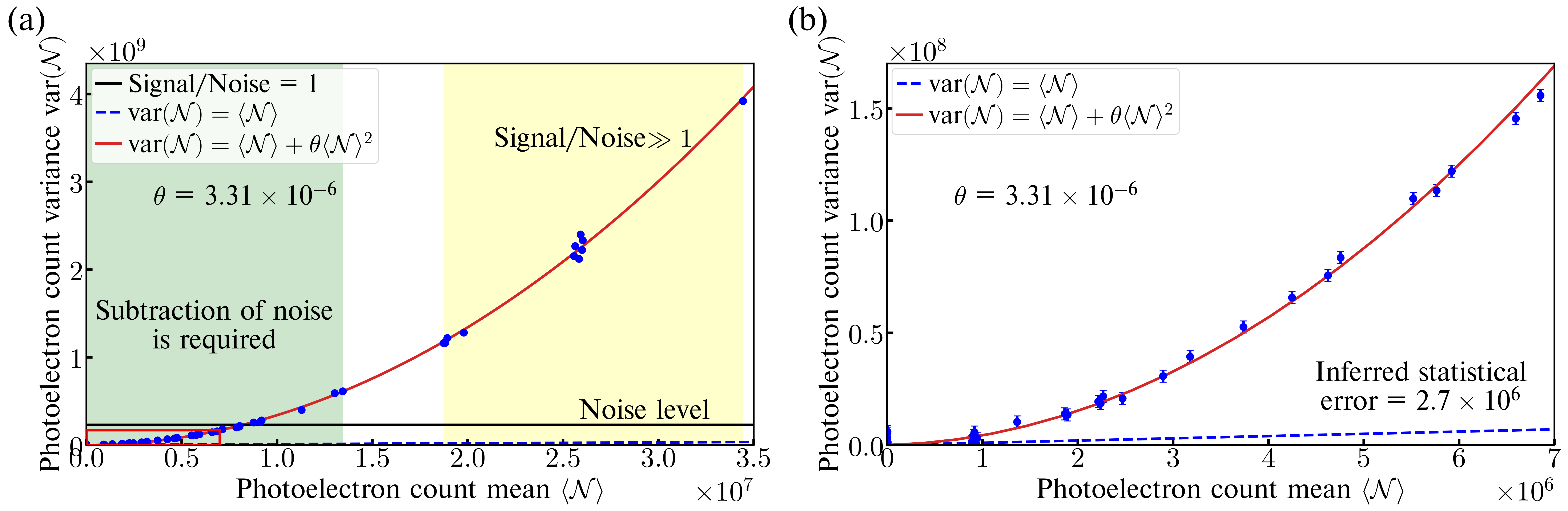
Figure 7: Photoelectron count variance $\mathrm{var}(\mathcal{N})$ as a function of photoelectron count mean $\langle\mathcal{N}\rangle$ for the test light source; $\langle\mathcal{N}\rangle$ was varied by using different neutral density filters. (a) The entire range of $\langle\mathcal{N}\rangle$, $\mathrm{var}(\mathcal{N})$. (b) The region corresponding to the values of $\mathrm{var}(\mathcal{N})$ generated by the undulator radiation in IOTA [highlighted by the red rectangle in (a)].

Appendix B Approximation of a Gaussian radiation profile

In this approximation, the following expression for the radiation field amplitude is used,

$$\mathcal{E}_{k,s}(\bm{\phi})=\sqrt{\frac{C_{s}}{(2\pi)^{3/2}\sigma_{k}\sigma_{r,x^{\prime}}\sigma_{r,y^{\prime}}}\exp[-\frac{(k-k_{0})^{2}}{2\sigma_{k}^{2}}-\frac{\phi_{x}^{2}}{2\sigma_{r,x^{\prime}}^{2}}-\frac{\phi_{y}^{2}}{2\sigma_{r,y^{\prime}}^{2}}\bigr{]}},$$ (37)

where $k_{0}$ refers to the center of the spectrum of the Gaussian radiation, $\sigma_{k}$ is the spectral rms width, $\sigma_{r,x^{\prime}}$ and $\sigma_{r,y^{\prime}}$ are the angular rms radiation sizes, $\sigma_{k}\ll 1/(\sigma_{x}\sigma_{r,x^{\prime}})$ and $\sigma_{k}\ll 1/(\sigma_{y}\sigma_{r,y^{\prime}})$, $C_{s}$ is a constant. An ideal detector is assumed — $\eta_{k,s}(\bm{\phi})=1$. In this case, for a Gaussian electron bunch, the following result can be obtained from Eq. 2,

$$M=(1-1/n_{e})^{-1}\sqrt{1+4\sigma_{k}^{2}\sigma_{z}^{2}}\\ \times\sqrt{1+4k_{0}^{2}(\sigma_{x}^{2}\sigma_{r,x^{\prime}}^{2}+\sigma_{x^{\prime}}^{2}\Sigma_{x}^{2})+\frac{\sigma_{x^{\prime}}^{2}}{\sigma_{r,x^{\prime}}^{2}}}\\ \times\sqrt{1+4k_{0}^{2}(\sigma_{y}^{2}\sigma_{r,y^{\prime}}^{2}+\sigma_{y^{\prime}}^{2}\Sigma_{y}^{2})+\frac{\sigma_{y^{\prime}}^{2}}{\sigma_{r,y^{\prime}}^{2}}}.$$ (38)

In the limit of zero electron beam divergence ($\sigma_{x^{\prime}},\sigma_{y^{\prime}}=0$), Eq. 38 coincides with [6, Eq. (17)], where this less general case was considered.

Appendix C Measurements with a test light source

The method of determining $\langle\mathcal{N}\rangle$ and $\mathrm{var}(\mathcal{N})$ by Eqs. 20 and 25 was tested with an independent test light source with known fluctuations. The test light source consisted of a fast laser diode ($1064\text{\,}\mathrm{n}\mathrm{m}$) with an amplifier, modulated by a pulse generator. The width of the light pulses and the repetition rate were very close to the experiment conditions in IOTA. However, the pulse-to-pulse fluctuations in the test light source were significantly greater than in the undulator radiation in IOTA, namely, $\mathrm{var}(\mathcal{N})=$4\text{\times}{10}^{9}\text{\,}$$ as opposed to $\mathrm{var}(\mathcal{N})=$01.5\text{\times}{10}^{8}\text{\,}$$ in IOTA. This also means that they were much greater than the instrumental noise level of our apparatus, $2.0\text{\times}{10}^{08}\text{\,}$. Therefore, we could reliably measure the relative fluctuations in the test light source, even without subtraction of the noise level, because it was negligible. The result was

$$\theta=\frac{\mathrm{var}(\mathcal{N})}{\langle\mathcal{N}\rangle^{2}}=$3.31\text{\times}{10}^{-06}\text{\,}$,$$ (39)

which corresponds to the rms value $1.82\text{\times}{10}^{-03}\text{\,}$. We believe that these fluctuations primarily came from the jitter in the pulse generator amplitude.

Further, we used neutral density filters to lower the number of photons detected by our apparatus. Neutral density filters are filters that have constant optical density in the wavelength region of interest. As they lower $\langle\mathcal{N}\rangle$ for the test light source, $\mathrm{var}(\mathcal{N})$ is lowered in the following known way,

$$\mathrm{var}(\mathcal{N})=\langle\mathcal{N}\rangle+\theta\langle\mathcal{N}\rangle^{2},$$ (40)

i.e., the relative fluctuations stay practically constant $\mathrm{var}(\mathcal{N})/\langle\mathcal{N}\rangle^{2}\approx\theta$, because they are caused by the pulse generator amplitude jitter, but at a very low $\langle\mathcal{N}\rangle$ the photon shot noise term [the first term in Eq. 40] may have a noticeable contribution, similar to Eq. 1. By using many different neutral density filters and their combinations we were able to record $\Delta$- and $\Sigma$-channel waveforms for a wide range of $\mathrm{var}(\mathcal{N})$, see Fig. 7(a), including the range observed in our experiment in IOTA, shown in Fig. 7(b) and highlighted by a red rectangle in Fig. 7(a).

In Figs. 7(a) and (b), the parameter $\theta$ of the red predicted curve was obtained in a configuration without any neutral density filters, when the detector noise and the photon shot noise were negligible, see Eq. 39. The blue fluctuation data points, obtained from the $\Delta$- and $\Sigma$-channel waveforms using Eqs. 20 and 25, agree with the red predicted curve in the entire range of $\mathrm{var}(\mathcal{N})$, including the range of Fig. 7(b) corresponding to the measurements in IOTA. This means that the method of extracting $\mathrm{var}(\mathcal{N})$ from the waveforms, described in Fig. 5 and Eq. 25, works well, and that the instrumental noise [$\mathrm{var}(\nu_{\Delta})=$2.0\text{\times}{10}^{08}\text{\,}$$] is indeed independent of the signal amplitude.

We estimated the statistical error of our measurement of photoelectron count variance in IOTA as the rms deviation of the fluctuation data points for the test light source from the predicted curve in Fig. 7(b). The error is $\pm$2.7\text{\times}{10}^{06}\text{\,}$$. It is used in the error bars in Figs. 6,7(b).

Appendix D Vertical emittance estimation for the flat beam via the Touschek beam lifetime

The beam lifetime could be reliably determined from the measured beam current $I$ as a function of time, as $\left|I/(\derivative*{I}{t})\right|$. During all of our measurements the beam current was measured with a DCCT current monitor, it was reported every second. Further, the waveforms from the wall-current monitor allowed us to see the distribution of the electrons among the 4 rf buckets in IOTA. We always corrected the DCCT current to only account for the main bucket. Typically, the combined population of the remaining 3 buckets was no more than a few percent. At the beam currents studied in our experiment ($13\text{\,}\mathrm{m}\mathrm{A}$), the beam lifetime is determined solely by Touschek scattering [44, 42]. In general, the momentum acceptance is a function of the position along the ring. It is limited by the longitudinal bucket size, $\delta_{\mathrm{rf}}$, and by the dynamic momentum aperture. A constant effective momentum acceptance $\delta_{\mathrm{acc}}^{(\mathrm{eff})}$ can be used [48] to describe the losses due to Touschek scattering. It is equal to or smaller than $\delta_{\mathrm{rf}}$. We used the approach described in [49, 50] to calculate the Touschek lifetime. Figure 8 shows the measured beam lifetime for the round beam, a calculation with the momentum acceptance limited only by the rf bucket size ($\delta_{\mathrm{rf}}=$2.8\text{\times}{10}^{-03}\text{\,}$$ in IOTA), and a calculation with an effective momentum acceptance $\delta_{\mathrm{acc}}^{(\mathrm{eff})}=$2.0\text{\times}{10}^{-03}\text{\,}$$.

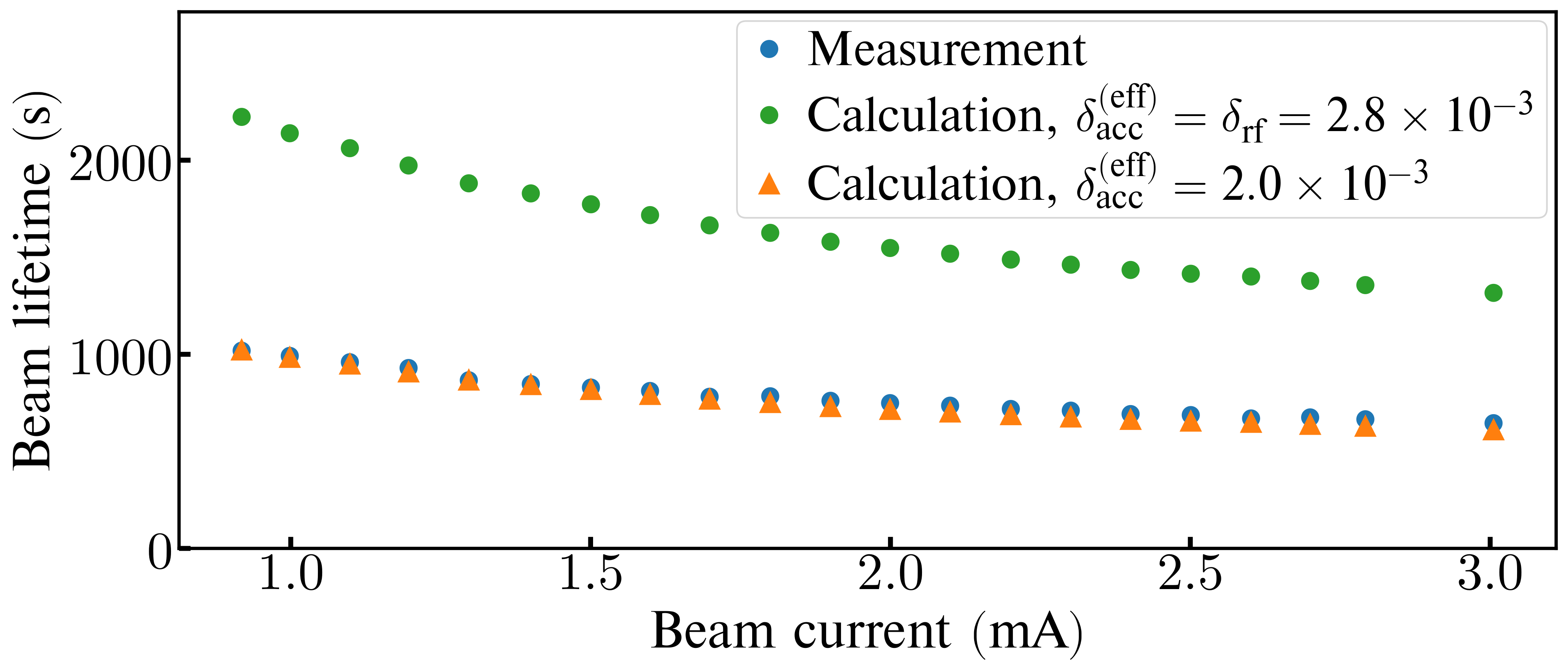
Figure 8: Lifetime of the round beam in IOTA as a function of beam current.

The calculation with $\delta_{\mathrm{acc}}^{(\mathrm{eff})}=$2.0\text{\times}{10}^{-03}\text{\,}$$ almost perfectly agrees with the measurement. The emittances and the beam lifetime of the round beam are known with good accuracy, the only unknown in this Touschek lifetime calculation for the round beam being $\delta_{\mathrm{acc}}^{(\mathrm{eff})}$. We believe that Fig. 8 illustrates that in IOTA $\delta_{\mathrm{acc}}^{(\mathrm{eff})}=$2.0\text{\times}{10}^{-03}\text{\,}$$.

Further, we can also apply this Touschek lifetime calculation (with $\delta_{\mathrm{acc}}^{(\mathrm{eff})}=$2.0\text{\times}{10}^{-03}\text{\,}$$) to the flat beam at a beam current of $2.66\text{\,}\mathrm{m}\mathrm{A}$, where we know the measured lifetime ($559\text{\,}\mathrm{s}$) and the horizontal emittance, but we cannot measure directly the small vertical emittance. We found the following value for the vertical emittance, $\epsilon_{y}=$9.6\text{\,}$\pm$1.2\text{\,}\mathrm{n}\mathrm{m}$$, to be compared with the fluctuations-based measurement, $\epsilon_{y}=$8.4\text{\,}$\pm$1.5\text{\,}\mathrm{n}\mathrm{m}$$. The $\pm$1.2\text{\,}\mathrm{n}\mathrm{m}$$ error in the lifetime-based $\epsilon_{y}$ estimate comes from the $\pm$50\text{\,}\mathrm{n}\mathrm{m}$$ uncertainty on $\epsilon_{x}$ of the flat beam. Other sources of error are much smaller: $\pm$5\text{\,}\mathrm{s}\mathrm{e}\mathrm{c}$$ uncertainty on the measured beam lifetime, uncertainties in the beam energy, Twiss-functions, and bunch length.

References

- Kim et al. [2017] K.-J. Kim, Z. Huang, and R. Lindberg, Synchrotron radiation and free-electron lasers (Cambridge University Press, 2017).
- Teich et al. [1990] M. C. Teich, T. Tanabe, T. C. Marshall, and J. Galayda, Statistical properties of wiggler and bending-magnet radiation from the Brookhaven Vacuum-Ultraviolet electron storage ring, Phys. Rev. Lett. 65, 3393 (1990).
- Sajaev [2000] V. Sajaev, Determination of longitudinal bunch profile using spectral fluctuations of incoherent radiation, Report No ANL/ASD/CP-100935 (Argonne National Laboratory, 2000).
- Sajaev [2004] V. Sajaev, Measurement of bunch length using spectral analysis of incoherent radiation fluctuations, in AIP Conf. Proc., Vol. 732 (AIP, 2004) pp. 73–87.
- Lobach et al. [2020a] I. Lobach, V. Lebedev, S. Nagaitsev, A. Romanov, G. Stancari, A. Valishev, A. Halavanau, Z. Huang, and K.-J. Kim, Statistical properties of spontaneous synchrotron radiation with arbitrary degree of coherence, Phys. Rev. Accel. Beams 23, 090703 (2020a).
- Sannibale et al. [2009] F. Sannibale, G. Stupakov, M. Zolotorev, D. Filippetto, and L. Jägerhofer, Absolute bunch length measurements by incoherent radiation fluctuation analysis, Phys. Rev. ST Accel. Beams 12, 032801 (2009).
- Catravas et al. [1999] P. Catravas, W. Leemans, J. Wurtele, M. Zolotorev, M. Babzien, I. Ben-Zvi, Z. Segalov, X.-J. Wang, and V. Yakimenko, Measurement of electron-beam bunch length and emittance using shot-noise-driven fluctuations in incoherent radiation, Phys. Rev. Lett. 82, 5261 (1999).
- Kim [1997] K.-J. Kim, Start-up noise in 3-D self-amplified spontaneous emission, Nucl. Instrum. Methods Phys. Res., Sect. A 393, 167 (1997).
- Benson and Madey [1985] S. Benson and J. M. Madey, Shot and quantum noise in free electron lasers, Nucl. Instrum. Methods Phys. Res., Sect. A 237, 55 (1985).
- Saldin et al. [2013] E. L. Saldin, E. Schneidmiller, and M. V. Yurkov, The physics of free electron lasers (Springer Science & Business Media, 2013).
- Pellegrini et al. [2016] C. Pellegrini, A. Marinelli, and S. Reiche, The physics of x-ray free-electron lasers, Rev. Mod. Phys. 88, 015006 (2016).
- Becker and Zubairy [1982] W. Becker and M. S. Zubairy, Photon statistics of a free-electron laser, Phys. Rev. A 25, 2200 (1982).
- Becker and McIver [1983a] W. Becker and J. McIver, Fully quantized many-particle theory of a free-electron laser, Phys. Rev. A 27, 1030 (1983a).
- Becker and McIver [1983b] W. Becker and J. McIver, Photon statistics of the free-electron-laser startup, Phys. Rev. A 28, 1838 (1983b).
- Chen and Madey [2001] T. Chen and J. M. Madey, Observation of sub-Poisson fluctuations in the intensity of the seventh coherent spontaneous harmonic emitted by a RF linac free-electron laser, Phys. Rev. Lett. 86, 5906 (2001).
- Chen [1999] T. Chen, Photon statistics of coherent harmonic radiation of a linac free electron laser, Ph.D. thesis, Duke University (1999).
- Park [2019] J.-W. Park, An Investigation of Possible Non-Standard Photon Statistics in a Free-Electron Laser, Ph.D. thesis, University of Hawaii at Manoa (2019).
- Antipov et al. [2017] S. Antipov, D. Broemmelsiek, D. Bruhwiler, D. Edstrom, E. Harms, V. Lebedev, J. Leibfritz, S. Nagaitsev, C.-S. Park, H. Piekarz, et al., IOTA (Integrable Optics Test Accelerator): facility and experimental beam physics program, J. Instrum. 12 (03), T03002.
- Hull and Williams [1925] A. W. Hull and N. Williams, Determination of elementary charge e from measurements of shot-effect, Phys. Rev. 25, 147 (1925).
- Johnson [1928] J. B. Johnson, Thermal agitation of electricity in conductors, Phys. Rev. 32, 97 (1928).
- Boussard [1986] D. Boussard, Schottky noise and beam transfer function diagnostics, Tech. Rep. CERN-SPS-86-11-ARF (1986).
- van der Meer [1989] S. van der Meer, Diagnostics with Schottky noise, in Frontiers of Particle Beams; Observation, Diagnosis and Correction (Springer, 1989) pp. 423–433.
- Caspers et al. [2007] F. Caspers, J. M. Jimenez, O. R. Jones, T. Kroyer, C. Vuitton, T. W. Hamerla, A. Jansson, J. Misek, R. J. Pasquinelli, P. Seifrid, et al., The 4.8 GHz LHC Schottky pick-up system, in 2007 IEEE Particle Accelerator Conference (PAC) (IEEE, 2007) pp. 4174–4176.
- Lobach et al. [2020b] I. Lobach, S. Nagaitsev, V. Lebedev, A. Romanov, G. Stancari, A. Valishev, A. Halavanau, Z. Huang, and K.-J. Kim, Transverse beam emittance measurement by undulator radiation power noise (2020b), arXiv:2012.00832 [physics.acc-ph] .
- Glauber [1963a] R. J. Glauber, The quantum theory of optical coherence, Phys. Rev. 130, 2529 (1963a).
- Glauber [1963b] R. J. Glauber, Coherent and incoherent states of the radiation field, Phys. Rev. 131, 2766 (1963b).
- Glauber [1951] R. J. Glauber, Some notes on multiple-boson processes, Phys. Rev. 84, 395 (1951).
- Lobach [2020a] I. Lobach, The source code for calculation of spectral-angular distribution of wiggler radiation, https://github.com/IharLobach/wigrad (2020a).
- Clarke [2004] J. A. Clarke, The science and technology of undulators and wigglers (Oxford University Press on Demand, 2004) pp. 66–67.
- Chubar et al. [2013] O. Chubar, A. Fluerasu, L. Berman, K. Kaznatcheev, and L. Wiegart, Wavefront propagation simulations for beamlines and experiments with "Synchrotron Radiation Workshop", in J. Phys. Conf. Ser., Vol. 425 (IOP Publishing, 2013) p. 162001.
- Lobach [2020b] I. Lobach, The source code for calculation of fluctuations in wiggler radiation, https://github.com/IharLobach/fur (2020b).
- Bjorken and Mtingwa [1982] J. D. Bjorken and S. K. Mtingwa, Intrabeam scattering, Part. Accel. 13, 115 (1982).
- Nagaitsev [2005] S. Nagaitsev, Intrabeam scattering formulas for fast numerical evaluation, Phys. Rev. ST Accel. Beams 8, 064403 (2005).
- Haïssinski [1973] J. Haïssinski, Exact longitudinal equilibrium distribution of stored electrons in the presence of self-fields, Il Nuovo Cimento B (1971-1996) 18, 72 (1973).
- Fellenz and Crisp [1998] B. Fellenz and J. Crisp, An improved resistive wall monitor, AIP Conference Proceedings 451, 446 (1998).
- Kuklev et al. [2019] N. Kuklev, J. Jarvis, Y. Kim, A. Romanov, J. Santucci, and G. Stancari, Synchrotron radiation beam diagnostics at IOTA — commissioning performance and upgrade efforts, in Proc. 10th International Particle Accelerator Conference (IPAC’19), Melbourne, Australia, 19-24 May 2019, International Particle Accelerator Conference No. 10 (JACoW Publishing, Geneva, Switzerland, 2019) pp. 2732–2735, https://doi.org/10.18429/JACoW-IPAC2019-WEPGW103.
- Lebedev and Bogacz [2010] V. A. Lebedev and S. Bogacz, Betatron motion with coupling of horizontal and vertical degrees of freedom, J. Instrum. 5 (10), P10010.
- [38] Hamamatsu InGaAs PIN photodiode G11193-10R, https://www.hamamatsu.com/us/en/product/type/G11193-10R/index.html, accessed: 2020-11-18.
- [39] Texas Instruments Wideband Operational Amplifier THS4303, http://www.ti.com/lit/ds/symlink/ths4304.pdf, accessed: 2020-11-18.
- Smith [2010] J. O. Smith, Physical audio signal processing: For virtual musical instruments and audio effects (W3K publishing, 2010).
- [41] MACOM H-9 Hybrid Junction, https://cdn.macom.com/datasheets/H-9.pdf, accessed: 2020-11-18.
- Lebedev [2020] V. Lebedev, Report on Single and Multiple Intrabeam Scattering Measurements in IOTA Ring in Fermilab, Report No FERMILAB-TM-2750-AD (Fermilab, 2020).
- Reiser and O’Shea [1994] M. Reiser and P. O’Shea, Theory and design of charged particle beams (Wiley Online Library, 1994) Chap. 6, pp. 483–486.
- Bernardini et al. [1963] C. Bernardini, G. F. Corazza, G. Di Giugno, G. Ghigo, J. Haissinski, P. Marin, R. Querzoli, and B. Touschek, Lifetime and beam size in a storage ring, Phys. Rev. Lett. 10, 407 (1963).
- Lebedev and Romanov [2015] V. Lebedev and A. Romanov, Optical stochastic cooling at the IOTA ring, Proceedings of COOL2015, Newport News VA , 123 (2015).
- Jarvis et al. [2018] J. D. Jarvis, V. Lebedev, H. Piekarz, A. L. Romanov, J. Ruan, M. B. Andorf, and P. Piot, Optical stochastic cooling experiment at the Fermilab IOTA ring (2018), arXiv:1808.07922 [physics.acc-ph] .
- Andorf et al. [2018] M. B. Andorf, V. A. Lebedev, J. Jarvis, and P. Piot, Computation and numerical simulation of focused undulator radiation for optical stochastic cooling, Phys. Rev. Accel. Beams 21, 100702 (2018).
- Carmignani [2014] N. Carmignani, Touschek Lifetime Studies and Optimization of the European Synchrotron Radiation Facility, Ph.D. thesis, Pisa U. (2014), pp. 25–26.
- Lebedev [2013] V. Lebedev, Intrabeam scattering, in Handbook of Accelerator Physics and Engineering, edited by A. Chao, K. Mess, M. Tigner, and F. Zimmermann (World Scientific, 2013) pp. 155–158.
- Piwinski [1999] A. Piwinski, The Touschek effect in strong focusing storage rings (1999), arXiv:physics/9903034 [physics.acc-ph] .