Imaginary Time Mean-Field Method for Collective Tunneling

Abstract

Background

Quantum tunneling in many-body systems is the subject of many experimental and theoretical studies in fields ranging from cold atoms to nuclear physics. However, theoretical description of quantum tunneling with strongly interacting particles, such as nucleons in atomic nuclei, remains a major challenge in quantum physics.

Purpose

An initial-value approach to tunneling accounting for the degrees of freedom of each interacting particle is highly desirable.

Methods

Inspired by existing methods to describe instantons with periodic solutions in imaginary time, we investigate the possibility to use an initial value approach to describe tunneling at the mean-field level. Real-time and imaginary-time Hartree dynamics are compared to the exact solution in the case of two particles in a two-well potential.

Results

Whereas real-time evolutions exhibit a spurious self-trapping effect preventing tunneling in strongly interacting systems, the imaginary-time-dependent mean-field method predicts tunneling rates in excellent agreement with the exact solution.

Conclusions

Being an initial-value method, it could be more suitable than approaches requiring periodic solutions to describe realistic systems such as heavy-ion fusion.

I Introduction

Quantum tunneling, allowing an object to pass a potential energy barrier, even when classically it does not have enough energy, is one of the most striking concepts of quantum physics. In Nature, it produces energy in stars via nuclear fusion, it heats the Earth’s interior by $\alpha-$decay, it produces new elements in nucleosynthesis, and it is believed to cause DNA mutations, ageing and cancer. Quantum tunneling also underpins many technological applications such as the tunneling electron microscope, FLASH memory, tunnel junctions in solar cells, and tunnel diodes in high speed devices. Although well-understood for simple systems such as electrons, the description of quantum tunneling for most systems (e.g., molecules, atomic nuclei, Bose-Einstein condensates) remains challenging due to their composite nature and the interaction between their constituents.

Several methods have been developed in recent years to describe tunneling of interacting particles. Due to the complexity of the problem, these methods are either limited to few-body systems Ahsan and Volya (2010); Hunn et al. (2013); Rontani (2013); Lundmark et al. (2015); Dobrzyniecki and Sowiński (2018) or they require approximations to the quantum many-body dynamics Umar and Oberacker (2009); Hagino and Takigawa (2012); Simenel et al. (2013); Fasshauer and Lode (2016); Wen and Nakatsukasa (2017); Simenel et al. (2017); Godbey et al. (2019); Lode et al. (2020). As a result, mean-field driven non-exponential decay Zhao et al. (2017); Alcala et al. (2017); Potnis et al. (2017) as well as substantial deviation from mean-field dynamics McLain et al. (2018) were found in cold atoms systems. Pairing effects have also been demonstrated in systems of two and three atoms Zürn et al. (2012, 2013); Gharashi and Blume (2015); Lundmark et al. (2015); Dobrzyniecki and Sowiński (2018, 2019). Indeed, two atoms can tunnel as a correlated pair when the interaction is strong and attractive Lundmark et al. (2015). Similar cluster tunneling is found in nuclear systems, e.g., in $\alpha-$decay. Despite being composed of four strongly interacting nucleons, $\alpha-$clusters can be approximated as inert particles due to the large difference between their ground-state and first excited state, thus reducing theoretical description of $\alpha-$decay to a single-particle tunneling problem. However, the situation is much more complicated with heavier systems which can encounter non-trivial many-body dynamics while tunneling, as, e.g., in spontaneous fission and in low-energy heavy-ion fusion reactions. Unlike cold atoms which tunnel sequentially or as small clusters, all nucleons are usually tunneling together as self-bound systems in such reactions. However, unlike in $\alpha-$decay, individual nucleonic degrees of freedom need to be accounted for. Indeed, microscopic nuclear dynamics calculations (see Simenel and Umar (2018) for a review) show that fusion is affected by nucleon transfer Vo-Phuoc et al. (2016); Godbey et al. (2017) leading to dissipation Williams et al. (2018); Simenel et al. (2020) and potentially decoherence Dasgupta et al. (2007) in many-body tunneling.

At present, there is no model of quantum many-body tunneling for strongly interacting systems such as nuclei that explicitly accounts for effects of dissipation or decoherence that are induced by nucleonic degrees of freedom. Nevertheless, early works based on instantons and path integral description of quantum mechanics opened the possibility for mean-field description of tunneling based on imaginary-time techniques Levit et al. (1980); Reinhardt (1981); Puddu and Negele (1987); Arve et al. (1987); Negele (1989); Skalski (2008). Direct implementation of this method, however, is challenging due to the difficulty to find quantum many-particle closed trajectories in imaginary time. To overcome this difficulty, we propose an initial value approach to describe tunneling through an imaginary time mean-field evolution akin to the way standard real-time mean-field evolution techniques such as time-dependent Hartree-Fock (TDHF) can be used to study vibrations (without requantization) (see, e.g., Simenel and Chomaz (2009); Avez and Simenel (2013)). This approach is tested in a simple toy-model where an exact solution exists, and where the evolution in classically forbidden region can be easily visualised. In particular, we show how tunneling probabilities can be extracted at the mean-field level. These predictions are compared with the exact solution for various strength of the interaction. The toy model has been chosen so that generalisations to more realistic systems are in principle feasible.

The two-well toy model is described in section II, where both exact and real-time mean-field dynamics are studied. The path integral approach and its application within the toy model are discussed in section III. The method to compute tunneling probabilities is introduced in section IV. Potential extensions and applications to more realistic systems are discussed in section V, before we conclude in section VI.

II Two-well model

We consider a simple toy model with two interacting distinguishable particles evolving according to the Hamiltonian

$$\hat{H}(1,2)=\hat{h}_{0}(1)+\hat{h}_{0}(2)+\hat{v}(1,2).$$ (1)

The single-particle Hamiltonian is written

$$\hat{h}_{0}=\alpha\ket{-}\bra{-},$$

where $\ket{-}$ is the excited state. Its ground-state $\ket{+}$ has energy 0. This corresponds to a two-well potential with two possible positions, $\ket{L}$ and $\ket{R}$, for a particle in the left and right well, respectively. These states are related to the eigenstates of $\hat{h}_{0}$ by $\ket{\pm}=\frac{1}{\sqrt{2}}(\ket{L}\pm\ket{R})$. In this model, a particle initially in one well can tunnel to the other well through a potential energy barrier decreasing with $\alpha$. The interaction is assumed to occur when both particles are in the same well with $\hat{v}(1,2)=\mu\,(\ket{LL}\bra{LL}+\ket{RR}\bra{RR})$, where $\mu$ is a parameter controlling the interaction strength. The initial state is chosen as $\ket{LL}$.

It is possible to extend this toy model by considering identical particles (bosons or fermions), adding more particles and modes, and using a more realistic interaction. Nevertheless, despite its simplicity this model accounts for the essential aspects of tunneling of interacting particles. Moreover, such simplifications allow for easier visualisation of the configuration space available to the system, and thus it gives us a better understanding of its dynamics. Most importantly, this model is exactly solvable analytically, thus providing a benchmark to test various approximations.

II.1 Exact dynamics

The exact evolution is determined from the time-evolution operator $\hat{U}=e^{-i\hat{H}t}$ (we set $\hbar=1$). The Hamiltonian of the two-well model is

$$\hat{H} = \alpha\left(\ket{-}_{1}\bra{-}_{1}\mathbb{1}_{2}+\mathbb{1}_{1}\ket{-}_{2}\bra{-}_{2}\right)$$

$$+\mu\left(\ket{LL}\bra{LL}+\ket{RR}\bra{RR}\right)$$

with $\ket{-}=\frac{1}{\sqrt{2}}(\ket{L}-\ket{R})$. The indices refer to particles 1 and 2. In the $\{L,R\}$ basis it is expressed as

$$\hat{H}=\,\,\blockarray{cccc}\ket{LL}&\ket{LR}\ket{RL}\ket{RR}\\ \block{(cccc)}\alpha+\mu-\alpha/2-\alpha/20\\ -\alpha/2\alpha 0-\alpha/2\\ -\alpha/20\alpha-\alpha/2\\ 0-\alpha/2-\alpha/2\alpha+\mu\\ \,\,\,\,\,.$$

In this basis, the operator counting the particles in the left well is

$$\hat{N}_{L}=\begin{pmatrix}2&0&0&0\\ 0&1&0&0\\ 0&0&1&0\\ 0&0&0&0\end{pmatrix}.$$

With the condition that the particles are initially in $\ket{LL}$, the state of the system at time $t$ is

$$\ket{\Psi}(t)=\exp(-i\hat{H}t)\ket{LL}.$$

The expectation value of $\hat{N}_{L}$ in this state can be expressed as

$$\langle\hat{N}_{L}\rangle=1+\frac{\beta-\mu}{2\beta}\cos(\frac{\beta+\mu}{2}t)+\frac{\beta+\mu}{2\beta}\cos(\frac{\beta-\mu}{2}t),$$ (2)

where $\beta=\sqrt{4\alpha^{2}+\mu^{2}}$. Note that $\langle\hat{N}_{L}\rangle$ does not depend on the sign of $\mu$, i.e., if the interaction is attractive ($\mu<0$) or repulsive ($\mu>0$). From now on, we set $\alpha=1$, so that the only parameter is the interaction strength $\mu$.

The exact evolution $\langle\hat{N}_{L}\rangle(t)$ is represented in Fig. 1 (blue solid line) for two values of $\mu$. The oscillatory behaviour shows that the particles can tunnel from the left well ($\langle\hat{N}_{L}\rangle/2=1$) to the right well ($\langle\hat{N}_{L}\rangle/2=0$). The effect of increasing the interaction strength $\mu$ is to slow down tunneling as the particles are found in the right well at a later time.

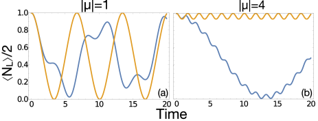
Figure 1: Exact solutions (blue solid lines) and real-time mean field predictions (orange solid lines) of $\langle\hat{N}_{L}\rangle(t)/2$ for (a) a weak interaction with $|\mu|=1$ and (b) a strong interaction with $|\mu|=4$. Time unit is fixed by our choice of $\alpha=1$.

II.2 Real time mean-field evolution

Approximations to describe the dynamics of quantum many-body systems are often based on the self-consistent mean-field theory, or time-dependent Hartree theory in the case of distinguishable particles. The latter assumes that the particles remain independent at all times, i.e., with a state $\ket{\Psi}=\ket{\psi_{1}}\otimes\ket{\psi_{2}}$. The Hamiltonian is then approximated by $\hat{H}_{H}(1,2)=\hat{h}_{H}(1)+\hat{h}_{H}(2)$ with time-dependent single-particle Hartree Hamiltonian

$$\hat{h}_{H}(i)=\hat{h}_{0}(i)+\bra{\psi_{j}}\hat{v}(1,2)\ket{\psi_{j}}$$

where $i,j=1,2$ and $j\neq i$. Note that in this form there is no spurious self-interaction.

As both particles are initially in the same state, they encounter the same mean-field evolution. As a result, they remain in identical states $\ket{\psi(t)}=L(t)\ket{L}+R(t)\ket{R}$ obeying the time-dependent Hartree equation

$$i\frac{d}{dt}\ket{\psi(t)}=\hat{h}_{H}(t)\ket{\psi(t)}.$$ (3)

The time-dependence of $\hat{h}_{H}(t)$ is due to its self-consistency. The equations of motion for $L(t)$ and $R(t)$ then become

$$i\frac{d}{dt}L =\frac{\alpha}{2}(L-R)+\mu L|L|^{2}\mbox{ and}$$ (4a)

$$i\frac{d}{dt}R =\frac{\alpha}{2}(R-L)+\mu R|R|^{2}.$$ (4b)

Let us define new coordinates $\theta\in[-\pi/2,\pi/2]$ and $\phi\in[-\pi,\pi]$:

$$\theta=\arcsin(|L|^{2}-|R|^{2})\mbox{ and }\phi=\arg(R/L).$$ (5)

This choice preserves the normalisation $|L|^{2}+|R|^{2}=1$. Both sets of coordinates are equivalent up to a global phase. From Eqs. (5) and the normalisation condition we can write

$$L=\sqrt{\frac{1+\sin\theta}{2}}e^{i\phi_{L}}\mbox{ and }R=\sqrt{\frac{1-\sin\theta}{2}}e^{i\phi_{R}}$$

where we have introduced the phases $\phi_{L,R}$. According to Eqs. (5), only their difference $\phi=\phi_{R}-\phi_{L}$ is relevant.

Inserting into Eqs. (4a) and (4b) gives

$$i\dot{\theta}\cos\theta-2(1+\sin\theta))\dot{\phi}_{L}= 1+\sin\theta-e^{i\phi}\cos\theta$$

$$+\mu(1+\sin\theta)^{2}$$ (6a)

$$-i\dot{\theta}\cos\theta-2(1-\sin\theta))\dot{\phi}_{R}= 1-\sin\theta-e^{-i\phi}\cos\theta$$

$$+\mu(1-\sin\theta)^{2},$$ (6b)

where we have set $\alpha=1$. Taking the imaginary part gives the first differential equation

$$\dot{\theta}=-\sin\phi.$$ (7)

Taking the real part of Eqs. (6a) and (6b) and rearranging gives the second differential equation

$$\dot{\phi}=\tan\theta\cos\phi+\mu\sin\theta.$$ (8)

Equations (7) and (8) provide a closed set of equations for the real-time mean-field dynamics of the system.

Solving these equations numerically with initial condition $(\theta,\phi)=(\frac{\pi}{2},0)$ corresponding to both particles in the left well, we get the real-time mean-field prediction for $\langle N_{L}\rangle(t)=1+\sin\theta(t)$ plotted in Fig. 1 (orange solid line). As in the exact case, the latter does not depend on the sign of $\mu$. Apart for the non-interacting case $\mu=0$ (for which mean-field dynamics is obviously exact), we see that mean-field predictions rapidly deviate from the exact solution. Although for $|\mu|\leq 2$, which we loosely refer to as the “weakly” interacting regime, tunneling is observed in the mean-field solution, a transition appears at $|\mu|=2$, above which (“strongly” interacting regime) the particles are “trapped” in one well, unable to tunnel completely to the other well. This spurious phenomenon, called “discrete self-trapping” Eilbeck et al. (1985); Smerzi et al. (1997); Milburn et al. (1997), illustrates the inability of real-time mean-field theory to describe tunneling dynamics in strongly interacting systems.

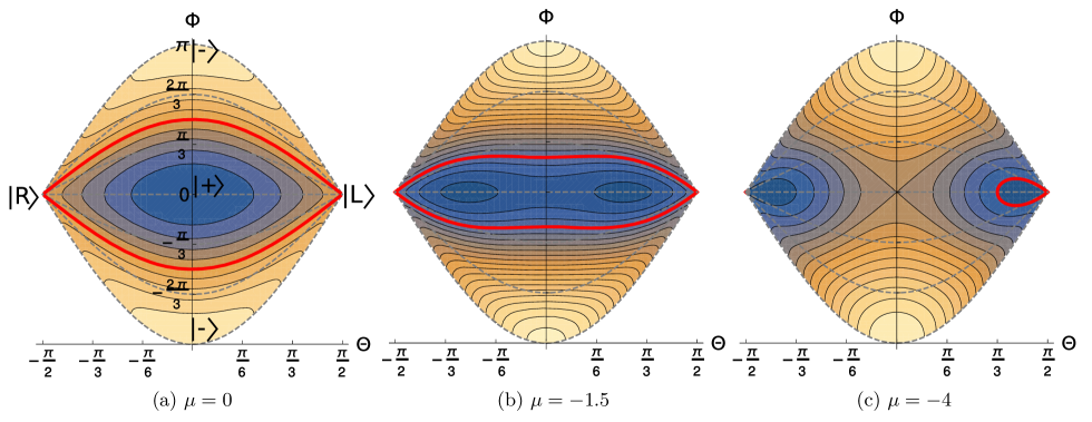
Figure 2: Mean-field energy contours are shown for (a) free particles, (b) a weak attraction, and (c) a strong attraction. Energy increases from blue to yellow. Solid red lines show mean-field trajectories starting from the left well. The dashed lines represent constant values of $\phi$.

II.3 Hartree energy

In order to investigate the origin of self-trapping, let us first determine the energy of the system in the mean-field approximation. Without interaction, the total energy is given by

$$K = \sum_{i=1}^{2}\bra{\psi_{i}}\hat{h}_{0}\ket{\psi_{i}}=\begin{pmatrix}L^{*}&R^{*}\end{pmatrix}\begin{pmatrix}1&-1\\ -1&1\end{pmatrix}\begin{pmatrix}L\\ R\end{pmatrix}$$

$$= 1-2\text{Re}[L^{*}R]=1-\cos\theta\cos\phi,$$

where we have used $\ket{\psi_{1,2}}=L\ket{L}+R\ket{R}$, Eqs. (5) and

$$\hat{h}_{0}=\frac{\alpha}{2}\begin{pmatrix}1&-1\\ -1&1\\ \end{pmatrix}$$

in the $\{\ket{L},\ket{R}\}$ basis, with our choice of $\alpha=1$.

With an interaction treated at the mean-field level, an additional term $U=\frac{1}{2}\sum_{i,j\neq i}\bra{\psi_{i}\psi_{j}}\hat{v}(1,2)\ket{\psi_{i}\psi_{j}}$ contributes to the total energy $E=K+U$. Using $\hat{v}(1,2)=\mu\,(\ket{LL}\bra{LL}+\ket{RR}\bra{RR})$, we get

$$U = \mu\begin{pmatrix}L^{*}&R^{*}\end{pmatrix}\begin{pmatrix}|L|^{2}&0\\ 0&|R|^{2}\end{pmatrix}\begin{pmatrix}L\\ R\end{pmatrix}$$

$$= \mu(|L|^{4}+|R|^{4})=\frac{\mu}{2}\left[1+\sin^{2}\theta\right].$$

As a result, the total (Hartree) energy is expressed as

$$E=1+\frac{\mu}{2}(1+\sin^{2}\theta)-\cos\theta\cos\phi$$ (9)

which is conserved under Eqs. (7) and (8).

II.4 Self-trapping

The self-trapping phenomenon can be understood by examining the mean-field dynamics of the system in the configuration space. The latter is entirely defined by the coordinates $\theta$ and $\phi$, allowing for a simple two-dimensional representation as in Figure 2(a) showing the position of the $\ket{L}$, $\ket{R}$ and $\ket{\pm}$ states.

Figuress 2(a-c) show contour plots of the Hartree energy in configuration space for various interaction strengths. As in the exact case, mean-field dynamics conserve total energy. The system is thus bound to follow iso-energy contour lines. We see that with no (Fig. 2(a)) or “weak” attraction (Fig. 2(b)), the system is able to go from one well to the other following a classically allowed path (thick solid red lines). However, in the case of “strong” attraction (Fig. 2(c)), there is no iso-energy contour line connecting both wells. The transition is classically forbidden, preventing tunneling and leading to self-trapping.

Self-trapping occurs when the states at $\theta=\pm\pi/2$ are not connected by any energy contour line in the $(\theta,\phi)$ plane. According to Eq. (9), the energy at $\theta=\pm\pi/2$ is

$$E_{1}=E\big{|}_{\theta=\pm\pi/2}=1+\mu,$$

while at $\theta=0$ it is

$$E_{2}(\phi)=E\big{|}_{\theta=0}=1+\frac{\mu}{2}-\cos\phi.$$

A condition for the system to tunnel from one well to another in the realtime mean-field dynamics is that there exist a $\phi$ for which $E_{2}(\phi)=E_{1}$ (otherwise the system is unable to cross the $\theta=0$ line). This is only possible for $\mu/2=-\cos\phi$, leading to the condition $|\mu|\leq 2$. Self-trapping then occurs when $|\mu|\geq 2$. This condition does not depend on the sign of $\mu$. Thus, despite the fact that the contour lines are different for attractive or repulsive interactions, self-trapping occurs in both cases for the same magnitude of the interaction strength.

II.5 “Weak” and “strong” interactions

Some comments are in order regarding the distinction between “weakly” and “strongly” interacting regimes. The situation in terms of realistic applications will depend on the system. For cold atoms, the interaction can be tuned experimentally and the “transition” region could then be explored.

For nuclear systems, in particular in the case of fusion, fission and cluster decay, the systems are expected to be well in the “strong” interaction regime. In our toy model, the energy splitting $\Delta E$ between the ground and first excited state of the exact Hamiltonian is the quantity that drives the tunneling rate. Arve et al. used a two-well potential with parameters adjusted to describe a typical fission problem, with energy splittings between the quasi-degenerate eigenstates of the order of $10^{-13}$ MeV for the ground-state, up to $10^{-2}$ MeV near the barrier Arve et al. (1987). In the two-well model we use, the energy splitting $\Delta E$ is $\sim\alpha^{2}/|\mu|$ for $|\mu|\gg\alpha$. The interaction $\mu$ is of the order of the binding energy per nucleon ($\sim 8$ MeV). To get similar splitting as Arve et al, we would then set $\alpha\sim 10^{-6}$ MeV for the ground state, up to $\sim 0.3$ MeV near the barrier. In any case, $\alpha$ remains smaller than $2|\mu|$ (recall that the transition appears at $|\mu|=2\alpha$), indicating a system clearly in the “strong” interaction regime.

III Path integral approach

Our goal is now to search for an initial-value mean-field based description of the system which would account for tunneling in the strongly interacting regime. Following Feynman’s many-path approach to quantum mechanics Feynman (1948), the amplitude of probability for the system to go from the state $\ket{i}$ at time $t_{i}$ to the state $\ket{f}$ at time $t_{f}$ is written as a path integral

$$\bra{f}\hat{U}(t_{f},t_{i})\ket{i}=\int D[\sigma]\exp(iS[\sigma]),$$

where $\hat{U}(t_{f},t_{i})$ is the evolution operator associated with the hamiltonian $\hat{H}$ of the system and $S[\sigma]$ is the action for the path $\sigma(t)$ in configuration space between $t_{i}$ and $t_{f}$.

III.1 Imaginary time-dependent mean-field equation

Though elegant, this path integral approach is often too complicated in practice and requires approximations such as the stationary phase approximation (SPA). For a single-particle following a classical path $\sigma(t)\equiv x(t)$, the SPA leads to the stationary action principle $\delta{S}=0$ of classical mechanics in which quantum tunneling is forbidden. Nevertheless, the latter can be recovered approximatively through a Wick rotation changing real time to imaginary time $t\rightarrow-i\tau$ Zichichi and Coleman (1979). Its effect is indeed to change the sign of the potential, thus allowing the system to explore classically forbidden regions. This approach is formally equivalent to the WKB semiclassical approximation Holstein and Swift (1982a, b).

For a many-particle system, mean-field equations can be recovered from the stationary action principle with the Dirac action

$$S=\int_{t_{i}}^{t_{f}}dt\bra{\Psi}i\partial_{t}-\hat{H}\ket{\Psi}$$ (10)

while restricting the variational space to independent particle states. However, as illustrated by our toy model, this theory does not account for tunneling in the strong interaction regime. Nevertheless, applying a Wick rotation should produce imaginary-time mean-field equations accounting for tunneling. Replacing $t\rightarrow-i\tau$ in Eq. (3) leads to an imaginary-time dependent Hartree equation

$$\frac{d}{d\tau}\ket{\psi(\tau)}=-\hat{h}_{H}(\tau)\ket{\psi(\tau)}.$$ (11)

As in real time evolution, computing observables $\langle\hat{Q}\rangle(\tau)$ also requires a conjugate state which we now define.

III.2 Wave-function of conjugate state

In real time, the wave-function of a single-particle conjugate state is given by $\tilde{\psi}(x,t)=\bra{\psi(t)}\ket{x}=\psi^{*}(x,t)$. It is convenient to write the wave-function as

$$\psi(x,t)=\sqrt{\rho(x,t)}e^{i\phi(x,t)},$$ (12)

with

$$\rho(x,t) =\tilde{\psi}(x,t)\psi(x,t)\,\,\mbox{ and}$$ (13a)

$$\phi(x,t) =\frac{1}{2i}\ln\left(\frac{\psi(x,t)}{\tilde{\psi}(x,t)}\right),$$ (13b)

leading to $\tilde{\psi}(x,t)=\sqrt{\rho(x,t)}e^{-i\phi(x,t)}$.

Imaginary-time evolution is obtained from a Wick rotation $t\rightarrow-i\tau$. This has a consequence for how the conjugate of a single-particle wave-function is defined. The conjugate is used to compute expectation values

$$\langle\hat{Q}\rangle(\tau)=\int dx\,\,\,\tilde{\psi}(x,\tau)\,Q(x,y)\,\psi(x,\tau)$$

which are transformed under the Wick rotation as

$$\langle\Psi(0)|e^{i\hat{H}t}\hat{Q}e^{-i\hat{H}t}|\Psi(0)\rangle\longrightarrow\langle\Psi(0)|e^{\hat{H}\tau}\hat{Q}e^{-\hat{H}\tau}|\Psi(0)\rangle.$$

The expectation value is then given by

$$\langle\hat{Q}\rangle(\tau)=\langle\Psi(-\tau)|\hat{Q}|\Psi(\tau)\rangle$$ (14)

implying

$$\tilde{\psi}(x,\tau)=\psi^{*}(x,-\tau).$$ (15)

In imaginary time, $\rho$ and $\phi$ become complex. It is easy to show from Eqs. (12), (13a) and (13b) that $\rho(\tau)=\rho^{*}(-\tau)$ and $\phi(\tau)=\phi^{*}(-\tau)$. As a result, Eq. (15) becomes

$$\tilde{\psi}(x,\tau)=\sqrt{\rho(x,\tau)}\exp(-i\phi(x,\tau)).$$ (16)

As a result, the conjugate in imaginary time has the same structure as in real time.

III.3 Classically forbidden region and final condition

Computing expectation values of observables in imaginary time thus requires both forward and backward evolutions. These are nevertheless initial value equations as only $|\Psi(0)\rangle$ is required to compute both evolutions in the classically forbidden region.

Criteria must be defined for where to “stop” the calculation. One (or several) observable $O_{f}$ can be used to define such criteria. The system needs then to be evolved in imaginary time until the condition (see footnote 1)

$$O(\tau)=\langle\psi_{0}|e^{\hat{H}\tau}\hat{O}e^{-\hat{H}\tau}|\psi_{0}\rangle=O_{f}$$

is reached. This defines the mean-field path from which the action and then the probability (see Sec. IV) to reach $\langle\hat{O}\rangle=O_{f}$ can be computed. For instance, $\hat{O}$ could be the quadrupole operator in fusion/fission problems, or the center of mass in cluster decay (see section V.0.3).

Note that the final state is not necessarily in the classically allowed region (in that case, however, a connection to real time dynamics cannot be performed). This is a major difference with earlier implementation of the imaginary-time mean-field approximation Levit et al. (1980) which required bounce solutions with the condition

$$\ket{\Psi(\tau)}=\ket{\Psi(-\tau)}.$$

III.4 Application to two-well model

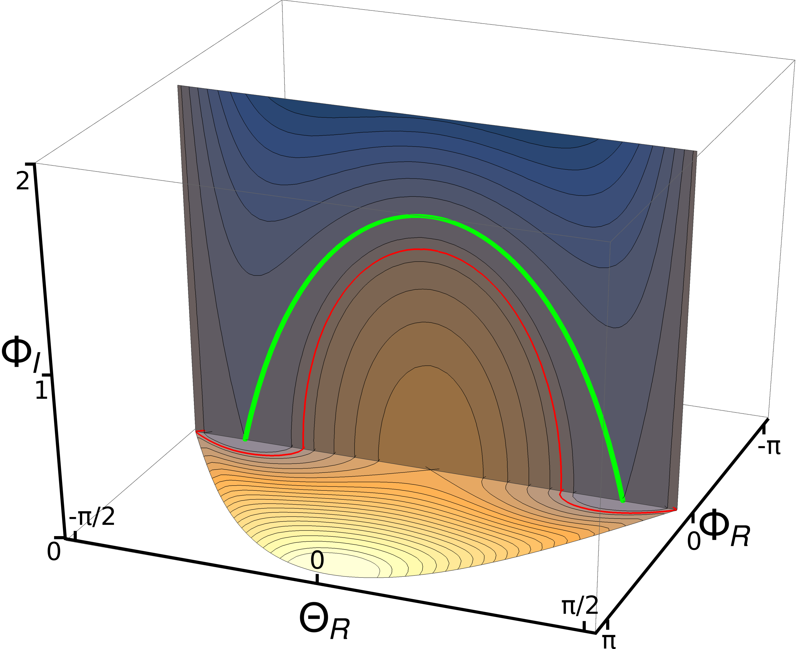
Figure 3: The real and imaginary-time mean-field energy is computed with $\mu=-3$ and is increasing from blue to yellow. The $(\theta_{R},\phi_{R})$ horizontal plane shows the energy for $\phi_{I}=\theta_{I}=0$. The $(\theta_{R},\phi_{I})$ vertical plane shows the energy for $\phi_{R}=\theta_{I}=0$. The red (respectively green) solid line shows an iso-energy contour connecting the left and right wells (resp. the left and right mean-field ground-states).

The equations of motion in imaginary time are obtained from a Witck rotation of Eqs. (7) and (8):

$$\frac{d\theta}{d\tau}=i\sin\phi\,\,\,\mbox{ and }\,\,\,\frac{d\phi}{d\tau}=-i\tan\theta\cos\phi-i\mu\sin\theta.$$ (17)

The coordinates $\theta=\theta_{R}+i\theta_{I}$ and $\phi=\phi_{R}+i\phi_{I}$ are now complex. The total energy of the system in the imaginary-time-dependent Hartree theory is still conserved and given by Eq. (9). As a result, as long as the initial condition is in the classically allowed region, i.e., with $\theta_{I}(t_{i})=\phi_{I}(t_{i})=0$, this energy remains real. This condition, together with the constant norm $\langle\psi(-\tau)|\psi(\tau)\rangle=1$ also impose relationships between $\theta$ and $\phi$.

Figure 3 shows this energy for a strongly attractive system. The horizontal plane gives the energy for real time evolution, as in Fig. 2. The vertical plane represents the energy for imaginary time evolution with $\phi_{R}=0$. It is now possible for the system to go from the left well to the right one following a combination of real and imaginary time evolutions (solid red line). This demonstrates the ability of imaginary time mean-field evolution to explore classically forbidden region through quantum tunneling.

IV Tunneling probability

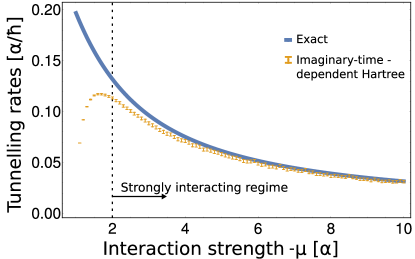
Figure 4: Exact (solid line) and imaginary-time-dependent mean-field (symbols) tunneling probabilities per unit of time (in units of $\alpha/\hbar$) are plotted as a function of the attraction strength $-\mu$ (in units of $\alpha$). Error bars correspond to numerical uncertainty of 1% in the action.

Now that we found mean-field tunneling paths, our next task is to calculate their associated tunneling probability per unit of time (tunneling rate) and compare it with the exact case.

Consider a mean-field evolution from $\ket{i}$ to $\ket{f}$ over a time $T$. In real-time, the probability to end up in $\ket{f}$ is $|\bra{f}\hat{U}(T)\ket{i}|^{2}=|e^{iS}|^{2}=1$ as the Dirac action in Eq. (10) for this path is real. The energy being constant, the global phase $ET$ is irrelevant.

In imaginary-time, this probability is now given by $|e^{iW}|^{2}$ with

$$W(T) = -\int_{0}^{T}d\tau\bra{\Psi}\partial_{\tau}\ket{\Psi}$$

$$= -\sum_{i=1}^{N}\int_{0}^{T}d\tau\bra{\psi_{i}(\tau)}\partialderivative{\tau}\ket{\psi_{i}(\tau)}$$

where $N$ is the number of particles. Using results from the previous section, we find

$$\bra{\psi}\partialderivative{\tau}\ket{\psi} =\int dx\,\left(\frac{1}{2}\partialderivative{\rho(x,\tau)}{\tau}+i\rho(x,\tau)\partialderivative{\phi(x,\tau)}{\tau}\right)$$

$$=\int dx\,i\rho(x,\tau)\partialderivative{\phi(x,\tau)}{\tau},$$

where we used the fact that $\int dx\,\rho(x,\tau)$ is constant.

In the toy model, the space integral $\int dx$ is simply replaced by a discrete sum $\sum_{L,R}$ over the left and right states, giving

$$W[T]=-i\int_{0}^{T}d\tau\,\,\left(\rho_{L}\partialderivative{\phi_{L}}{\tau}+\rho_{R}\partialderivative{\phi_{R}}{\tau}\right)$$

where

$$\rho_{L}=\frac{1+\sin\theta}{2}\mbox{ and }\rho_{R}=\frac{1-\sin\theta}{2}.$$

Once again, only the relative phase $\phi=\phi_{R}-\phi_{L}$ matters, thus we set $\phi_{R}=\phi/2$ and $\phi_{L}=-\phi/2$, giving

$$W[T]=\frac{i}{2}\int_{0}^{T}d\tau\,\,\sin\theta\partial_{\tau}\phi.$$

Using the second equation of motion (17), we finally get

$$W[T]=\frac{1}{2}\int_{0}^{T}d\tau\,\,(\tan\theta\cos\phi+\mu\sin\theta)\sin\theta.$$

Up to an irrelevant global phase, the tunneling probability amplitude for an imaginary-time-dependent mean-field path $\Psi(\tau)$ connecting the two wells is then given by

$$e^{iS[\Psi]}\equiv e^{-i\int d\tau\bra{\Psi}\partial_{\tau}\ket{\Psi}}=e^{\frac{i}{2}\int_{0}^{T}d\tau\,(\tan\theta\cos\phi+\mu\sin\theta)\sin\theta}.$$

As $\theta$ and $\phi$ are now complex quantities, the tunneling probability $|e^{iS[\Psi]}|^{2}$ associated with this path can be less than one.

By analogy with the standard semi-classical treatment of $\alpha-$decay Gamow (1928), the tunneling rate is given by the tunneling probability multiplied by the frequency at which the system “hits” the potential barrier, i.e., the frequency of the oscillation observed in mean-field trapping [see orange line in Fig. 1(b)]. As the system may tunnel from different configurations along a real-time iso-energy contour [see solid red line in Fig. 2(c)], the tunneling rate is in principle obtained by averaging over the associated imaginary-time paths. To a good approximation, this corresponds to the tunneling rate for the path connecting the left and right degenerate mean-field ground-states, indicated by the solid green line in Fig. 3.

In the exact case, the tunneling rate is simply given by twice the frequency at which the system oscillates between left and right wells. As shown in Eq. (2), this oscillation has two modes at $\omega_{\pm}=\frac{\sqrt{4\alpha^{2}+\mu^{2}}\pm|\mu|}{2\pi}$. Only the lowest frequency is associated with tunneling, giving an exact tunneling rate $2\omega_{-}=\frac{2}{\pi}\Delta E$ where $\Delta E=\frac{\sqrt{4\alpha^{2}+\mu^{2}}-|\mu|}{2}\xrightarrow[|\mu|\gg\alpha]{}\frac{\alpha^{2}}{|\mu|}$ is the energy difference between the ground and first excited states.

The mean-field and exact tunneling rates are compared in Fig. 4. Although the imaginary-time mean-field predictions are wrong for weakly interacting ($|\mu|<2$) systems – in which case the real-time mean-field prediction can be used anyway – it is in excellent agreement with the exact case in the strongly interacting regime, reproducing well the slowing down of tunneling with increased interactions.

V Towards realistic applications

The purpose of the two-well model is to illustrate the imaginary time mean-field method and compare with an exact solution (which would be hard to obtain with more realistic models). This is of course a first step and for the method to be useful, its applicability to more realistic systems needs to be demonstrated.

V.0.1 Cartesian grids

The toy model has only two states per particle, while the single-particle Hilbert space for a one-dimensional discretised cartesian grid has as many states as the number of points in the grid – typically $\sim 100$. Naturally, numerical simulations with non-unitary evolution operators such as $\exp(\pm\hat{H}\tau)$ present additional technical challenges in terms of stability and convergence. The generalisation from one to three dimensions will be another computational challenge, though it does not bring additional formal difficulty in terms of the algorithm itself.

V.0.2 Spin and exchange terms

Other extensions include the inclusion of spin and exchange terms. Spin $1/2$ degrees of freedom can be accounted for in the same way as in real-time calculations where each single-particle is treated as a 2-spinor $(\varphi_{\uparrow}(\mathbf{r}),\varphi_{\downarrow}(\mathbf{r}))$. An exchange (Fock) term also appears in the case of identical particles. In general, it is non-local and often requires a major extra computation cost. However, in the case of contact interactions (often used in cold atoms systems as well as in nuclear physics, e.g., with the Skyrme effective interaction Skyrme (1956)), the exchange terms are easily accounted for. For Coulomb interactions, the exchange term can also be included via the Slater approximation.

V.0.3 Potential applications

Several applications could be considered:

• Interacting particles in an external potential
  Cluster dynamics such as $\alpha-$decay or emission of atom clusters can be studied with an external potential. In this case, the external potential simulates the mean-field of the particles which do not belong to the cluster, while each particle of the cluster is treated explicitly. One could study the effect of the internal degrees of freedom of the cluster while it tunnels as a whole. In this case the classically forbidden region could be defined as the turning points of the external potential in the usual way.

• Merging of two self-bound systems
  A typical example is the fusion of two atomic nuclei. Note that the nuclei are self-bound and thus there is no external potential in this problem, i.e., $h_{0}$ only contains the kinetic energy of the nucleons. The nuclei are bound thanks to their strong nuclear interaction. The Coulomb barrier preventing fusion in the classical case is produced by the competition of long-range Coulomb repulsion between protons and the short range nuclear attraction of all nucleons, both terms being part of the interaction $v(1,2)$. In this case, the real-time mean-field dynamics is only able to reach fusion if the kinetic energy at large distance exceeds the Coulomb barrier height (for a central collision). At lower energy, tunneling will be obtained through the imaginary time mean-field method.

  As illustrated by the red line in Fig. 3, the system may explore different configurations through real-time dynamics, with each of these configurations potentially serving as initial condition for the imaginary time evolution. In principle, a weighting of each possibility should be determined. In practice, however, the transmission through the barrier is expected to be dominated by the trajectory starting from the distance of closest approach.

• Scission of a self-bound metastable system
  Self-bound systems can be in a local minimum of their potential energy surface, with more stable configurations corresponding to disconnected fragments. This is the case of fission in heavy nuclei. Here, again, the parent nucleus is self-bound and no external potential is required ($h_{0}$ only contains a kinetic energy term). In the case of spontaneous fission in particular, all directions in the multidimensional potential energy surface are classically forbidden, thus the initial condition for the imaginary time evolution is well defined.

VI Conclusions

Theoretical description of tunneling in strongly interacting systems such as atomic nuclei remains a challenging problem. Standard real-time mean-field approaches are unable to account for many-body tunneling due to spurious “self-trapping”. Using a simple model with two particles in a two-well potential, we demonstrated the possibility to overcome this limitation by allowing imaginary-time mean-field evolution. Tunneling probabilities are in excellent agreement with the exact solution in the strongly interacting regime.

These results are promising and encourage applications to more realistic systems. A first natural extension is to increase the number of modes, e.g., using cartesian grids with one or more dimensions. Computational effort only increases linearly with the number of particles at the mean-field level, so simulating tunneling dynamics of larger systems (out of reach to exact and few-body techniques) should not be an issue. The imaginary-time mean-field equations could also be extended to include pairing correlations Levit (2020).