Speaker Recognition Based on Deep Learning: An Overview

Abstract

Speaker recognition is a task of identifying persons from their voices. Recently, deep learning has dramatically revolutionized speaker recognition. However, there is lack of comprehensive reviews on the exciting progress. In this paper, we review several major subtasks of speaker recognition, including speaker verification, identification, diarization, and robust speaker recognition, with a focus on deep-learning-based methods. Because the major advantage of deep learning over conventional methods is its representation ability, which is able to produce highly abstract embedding features from utterances, we first pay close attention to deep-learning-based speaker feature extraction, including the inputs, network structures, temporal pooling strategies, and objective functions respectively, which are the fundamental components of many speaker recognition subtasks. Then, we make an overview of speaker diarization, with an emphasis of recent supervised, end-to-end, and online diarization. Finally, we survey robust speaker recognition from the perspectives of domain adaptation and speech enhancement, which are two major approaches of dealing with domain mismatch and noise problems. Popular and recently released corpora are listed at the end of the paper.

1 Introduction

It is known that a speaker’s voice contains personal traits of the speaker, given the unique pronunciation organs and speaking manner of the speaker, e.g. the unique vocal tract shape, larynx size, accent, and rhythm [1]. Therefore, it is possible to identify a speaker from his/her voice automatically via a computer. This technology is termed as automatic speaker recognition, which is the core topic of this paper. We do not discuss speaker recognition by humans. Speaker recognition is a fundamental task of speech processing, and finds its wide applications in real-world scenarios. For example, it is used for the voice-based authentication of personal smart devices, such as cellular phones, vehicles, and laptops. It guarantees the transaction security of bank trading and remote payment. It has been widely applied to forensics for investigating a suspect to be guilty or non-guilty [1, 2, 3], or surveillance and automatic identity tagging [4]. It is important in audio-based information retrieval for broadcast news, meeting recordings and telephone calls. It can also serve as a frontend of automatic speech recognition (ASR) for improving the transcription performance of multi-speaker conversations.

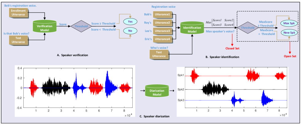
Figure 1: Flowcharts of speaker verification, speaker identification, and speaker diarization. Fig. A describes speaker verification, which is a task of verifying whether a test utterance and an enrollment utterance are uttered by the same speaker via comparing the similarity score of the utterances with a pre-defined threshold. Fig. B describes speaker identification, which is a task of determining the speaker identity of a test utterance from a set of speakers. If the utterance must be produced from the set of the speakers, then it is a closed set identification problem; otherwise, it is an open set problem. Fig. C describes speaker diarization, which addresses the problem of “who spoke when”, i.e., partitioning a conversation recording into several speech recordings, each of which belongs to a single speaker.

The research on speaker recognition can be dated back to at least 1960s [5]. In the following forty years, many advanced technologies promoted the development of speaker recognition. For example, a number of acoustic features (e.g. the linear predictive cepstral coefficients, the perceptual linear prediction coefficient, and the mel-frequency cepstral coefficients) and template models (e.g. vector quantization, and dynamic time warping) have been applied, see [1] for the details. Later on, [6] proposed the Gaussian mixture model based universal background model (GMM-UBM), which has been the foundation of speaker recognition for more than ten years since year 2000. Several representative models based on GMM-UBM have been developed, including the applications of support vector machines [7] and joint factor analysis [8]. Among the models, the GMM-UBM/i-vector frontend [9] with probabilistic linear discriminant analysis (PLDA) backend [10, 11] provided the state-of-the-art performance for several years, until the new era of deep learning based speaker recognition.

Recently, motivated by the powerful feature extraction capability of deep neural networks (DNNs), a lot of deep learning based speaker recognition methods were proposed [12, 13, 14] right after the great success of deep learning based speech recognition, which significantly boosts the performance of speaker recognition to a new level, even in wild environments [15, 16].

In this survey article, we give a comprehensive overview to the deep learning based speaker recognition methods in terms of the vital subtasks and research topics, including speaker verification, identification, diarization, and robust speaker recognition. By doing the survey, we hope to provide a useful resource for the speaker recognition community. The main contributions of this paper are summarized as follows:

• We summarize deep learning based speaker feature extraction techniques for speaker verification and identification, from the aspects of inputs, network structures, temporal pooling strategies, and objective functions which are also the fundamental components of many other speaker recognition subtasks beyond speaker verification and identification.

• We make an overview to the deep learning based speaker diarization, with an emphasis of recent supervised, end-to-end, and online diarization.

• We survey robust speaker recognition from the perspectives of domain adaptation and speech enhancement, which are two major approaches to deal with domain mismatch and noise problems.

In the last two decades, many excellent overviews on speaker recognition have been published. This paper is fundamentally different from previous overviews. First, this paper focuses on the recently development of deep learning based speaker recognition techniques, while most previous overviews are based on traditional speaker recognition methods [1, 17, 4, 18, 19, 20, 21]. Although [22, 23] summarized deep learning based speaker recognition methods in certain aspects, our paper summarizes different subtasks and topics from new perspectives. Specifically, [22] presents an overview to the potential threats of adversarial attacks to speaker verification as well as the spoofing countermeasures, which is not the focus of this overview. We provide a broad and comprehensive overview to a wide aspects of speaker verification, speaker diarization, domain adaptation, most of which have not been mentioned in [23].

This article is targeted at three categories of readers: The beginners who wish to study speaker recognition, the researchers who want to learn the whole picture of speaker recognition based on deep learning, and the engineers who need to understand or implement specific algorithms for their speaker recognition related products. In addition, we assume that the readers have basic knowledge of speech signal processing, machine leaning and pattern recognition.

The rest of the survey is organized as follows. In Section 2, we give a general overview and define some notations. In Sections 3 to 10, we survey the deep learning based speaker recognition methods in various aspects. In Section 11, we summarize some speaker recognition challenges and publicly available data. Finally, we conclude this article in Section 12.

2 Overview and scope

This overview summarizes four major research branches of speaker recognition, which are speaker verification, identification, diarization, and robust speaker recognition respectively. The flowcharts of the first three branches are described in Fig. 1, while robust speaker recognition deals with the challenges of noise and domain mismatch problems. The contents of the overview are organized in Fig. 2, which are described briefly as follows.

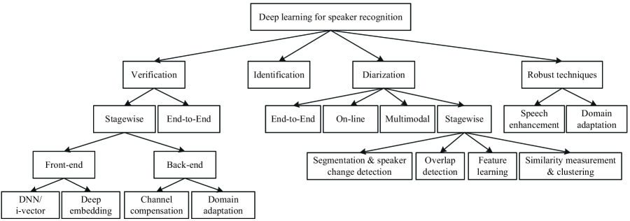
Figure 2: Overview of deep learning based speaker recognition.

Speaker verification aims at verifying whether an utterance is pronounced by a hypothesized speaker based on his/her pre-recorded utterances. Speaker verification algorithms can be categorized into stage-wise and end-to-end ones. A stage-wise speaker verification system usually consists of a front-end for the extraction of speaker features and a back-end for the similarity calculation of speaker features. The front-end transforms an utterance in time domain or time-frequency domain into a high-dimensional feature vector. It accounts for the recent advantage of the deep learning based speaker recognition. We survey the research on the front-end comprehensively in Sections 3 to 7. The back-end first calculates a similarity score between enrollment and test speaker features and then compare the score with a threshold:

$$f(\mathbf{x}^{e},\mathbf{x}^{t};\mathbf{w})\mathop{\gtrless}\limits_{H_{1}}^{H_{0}}\xi$$ (1)

where $f(\cdot)$ denotes a function for calculating the similarity, $\mathbf{w}$ stands for the parameters of the back-end, $\mathbf{x}^{e}$ and $\mathbf{x}^{t}$ are the enrollment and test speaker features respectively, $\xi$ is the threshold, $H_{0}$ represents the hypothesis of $\mathbf{x}^{e}$ and $\mathbf{x}^{t}$ belonging to the same speaker, and $H_{1}$ is the opposite hypothesis of $H_{0}$. One of the major responsibilities of the back-end is to compensate the channel variability and reduce interferences, e.g. language mismatch. Because most back-ends aim at alleviating the interferences, which belongs to the problem of robust speaker recognition, we put the overview of the back-ends in Section 10.

In contrast to the stage-wise techniques, end-to-end speaker verification takes a pair of speech utterances as the input, and produces their similarity score directly. Because a fundamental difference between the end-to-end speaker verification and the deep embedding techniques in the stage-wise speaker verification is the loss function, we mainly summarize the loss functions of the end-to-end speaker verification in Section 8.

Speaker identification aims at detecting the speaker identity of a test utterance $\mathbf{x}^{t}$ from an enrollment database $\{\mathbf{x}_{k}^{e}|k=1,2,\cdots,K\}$ by:

$$k^{*}=\arg\max_{k}\{f(\mathbf{x}^{e}_{1},\mathbf{x}^{t};\mathbf{w}),f(\mathbf{x}^{e}_{2},\mathbf{x}^{t};\mathbf{w}),\cdots,f(\mathbf{x}^{e}_{K},\mathbf{x}^{t};\mathbf{w})\}$$ (2)

where $K>1$ denotes the number of the enrollment speakers. If $\mathbf{x}^{t}$ can never be out of the $K$ registered speakers, then the speaker identification problem is a closed set problem; otherwise, it is an open set problem. Comparing (1) with (2), we see that speaker verification is a special case of the open set speaker identification problem with $K=1$, therefore, it is possible that the fundamental techniques of speaker identification and verification are similar, as what we have observed in [24, 25, 26, 27, 28]. Taking this point into consideration, we make a joint overview to speaker verification and identification with an emphasis on the former.

Speaker diarization addresses the problem of “who spoke when”, which is a process of partitioning a conversation recording into several speech recordings, each of which belongs to a single speaker. As shown in Fig. 2, a conventional framework of speaker diarization is stage-wise with multiple modules. Although the stage-wise speaker verification and diarization share some common modules, e.g. voice activity detection and speaker feature extraction, they have many differences. First, speaker verification assumes that each utterance belongs to a single speaker, while the number of speakers of a conversation in speaker diarization changes case by case. Moreover, speaker verification has an explicit registration/enrollment procedure, while speaker diarization intends to detect speakers on-the-fly without an enrollment procedure. At last, overlapped speech is one of the biggest challenges of speaker diarization, while speaker verification usually assumes that the enrollment or test utterance contains a single speaker only. Therefore, we focus on reviewing the work on the above distinguished properties of the stage-wise speaker diarization in Section 9. Recently, end-to-end speaker diarization, which outputs the diarization result directly, attracted much attention. Online speaker diarization, which meets the requirement of real-world applications, is also an emerging direction. Furthermore, multimodal speaker diarization, which integrates speech with video or text signals, was also studied extensively. We review the aforementioned end-to-end, online, and multimodal speaker diarization techniques in Section 9.

Besides, speech is easily contaminated by additive noise, reverberation, channel distortions. Therefore, robust speaker recognition is also one of the main topics. It mainly includes speech enhancement and domain adaptation techniques, which will be summarized in detail in Section 10. At last, we survey benchmark corpora in Section 11.

To summarize, the aforementioned contents will be organized as listed in Table 1. The notations are summarized in Table 2.

Table 1: Organization of the contents of this paper.

Sections	Contents
1, 2	Introduction and brief overview.
3, 4, 5, 6, 7	Speaker feature extraction.
8	The loss functions of the end-to-end speaker verification.
9	Speaker diarization.
10	Robust speaker recognition.
11	Benchmark corpora.
12	Conclusions and discussions.

Table 2: Summary of the notations in this paper.

Notation	Description
$\mathbb{R}$	Set of real numbers
$\mathbb{R}^{d}$	Set of $d$-dimensional real-valued vectors
$\mathbb{R}^{d_{1}\times d_{2}}$	Set of $d_{1}\times d_{2}$ real-valued matrices
$\mathcal{Y}$	Set of acoustic features
$\mathcal{H}$	Set of the last frame-level hidden layer’s outputs
$\mathcal{E}$	Set of embeddings
$\mathcal{X}$	Set of the inputs to loss functions
$\mathcal{L}$	The symbol of loss functions
$\mathbf{y}$	A frame acoustic feature
$\mathbf{h}$	A hidden feature of the last frame-level layer’s output
$\mathbf{e}$	An embedding feature of the embedding layer’s output
$\mathbf{x}$	An input feature to loss functions
$\mathbf{u}$	An output of the temporal pooling layer
$t,\,T$	Index and total number of frames in an utterance
$i,\,I$	Index and total number of the utterance
$j,\,J$	Index and total number of speakers in the training set
$\|\cdot\|$	The $\ell_{2}$ norm
$\odot$	The Hadamard product
$\delta(\cdot)$	Indicator function
$(\cdot)^{T}$	The transform of matrix or vector

3 Speaker feature extraction with DNN/i-vector

In this section, we first introduce two main streams of the deep learning based improvement to the i-vector framework in Section 3.1, and then comprehensively review the two streams in Sections 3.2 and 3.3 respectively. Finally, we make some discussions to the DNN/i-vector in Section 3.4.

Figure 3: The traditional GMM/i-vector framework. The term MFCC denotes Mel-frequency cepstral coefficent.

3.1 From GMM/i-vector to DNN/i-vector

The performance of the conventional GMM-UBM based speaker recognition is largely affected by the speaker and channel variations of utterances. To address this issue, [9] proposed to reduce the high-dimensional GMM-UBM supervectors into low-dimensional vectors, named i-vectors by factor analysis. The GMM/i-vector system eliminates the within-speaker and channel variabilities effectively, which leads to significant performance improvement.

The GMM/i-vector system is shown in Fig. 3. We assume that $\mathcal{Y}=\{\mathbf{y}_{t}^{(i)}\in\mathbb{R}^{d_{1}}|t=1,2,\cdots,T\}$ represents the $i$th ($i=1,2,\cdots,I$ ) utterance of $T$ successive Mel-frequency cepstral coefficent (MFCC) frames, and $\Omega=\{\omega_{c}\in\mathbb{R},\bm{\mu}_{c}\in\mathbb{R}^{d_{1}},\bm{\Sigma}_{c}\in\mathbb{R}^{d_{1}\times d_{1}}|c=1,2,\cdots,C\}$ ($\omega_{c}\geq 0$ for all $c$, and $\sum_{c=1}^{C}\omega_{c}=1$) denotes a GMM-UBM model where $C$ is the total number of components and $\omega_{c}$, $\bm{\mu}_{c}$ and $\bm{\Sigma}_{c}$ are the weight, mean, and covariance matrix of the $c$th component respectively. Then, $\mathbf{y}_{t}^{(i)}$ is assumed to be generated by the following distribution [12, 29]:

$$\mathbf{y}_{t}^{(i)}\sim\sum_{c=1}^{C}\omega_{c}N(\bm{\mu}_{c}+\mathbf{T}_{c}\bm{\upsilon}^{(i)},\bm{\Sigma}_{c})$$ (3)

where $\{\mathbf{T}_{c}\}_{c=1}^{C}$ is a so called total variability subspace, $\bm{\upsilon}^{(i)}$ is a segment-specific standard normal-distributed latent vector. The i-vector used to represent the speech signal is the maximum a posterior (MAP) point estimate of the latent vector $\bm{\upsilon}^{(i)}$, and it can be regarded as a kind of “speaker embedding”.

Given a speech segment, the following sufficient statistics can be accumulated from the GMM-UBM:

$$N_{c}^{(i)}=\sum_{t=1}^{T}p(c|\mathbf{y}_{t}^{(i)})$$ (4)

$$\mathbf{f}_{c}^{(i)}=\sum_{t=1}^{T}p(c|\mathbf{y}_{t}^{(i)})\mathbf{y}_{t}^{(i)}$$ (5)

$$\mathbf{S}_{c}^{(i)}=\sum_{t=1}^{T}p(c|\mathbf{y}_{t}^{(i)})\mathbf{y}_{t}^{(i)}(\mathbf{y}_{t}^{(i)})^{T}$$ (6)

where $p(c|\mathbf{y}_{t}^{(i)})=\frac{\omega_{c}N(\mathbf{y}_{t}^{(i)};\bm{\mu}_{c},\bm{\Sigma}_{c})}{\sum_{c^{\prime}=1}^{C}\omega_{c}N(\mathbf{y}_{t}^{(i)};\bm{\mu}_{c^{\prime}},\bm{\Sigma}_{c^{\prime}})}$ denotes the posterior probability of $\mathbf{y}_{t}^{(i)}$ against the $c$th Gaussian component. These sufficient statistics are all that are needed to train the subspace $\{\mathbf{T}_{c}\}_{c=1}^{C}$ and extract the i-vector $\bm{\upsilon}^{(i)}$ [12]. See [9, 30] for the details of training $\mathbf{T}_{c}$ and estimating the i-vectors.

Motivated by the success of deep learning for speech recognition, many efforts have been made to replace the GMM-UBM module of the GMM/i-vector system by DNN, which can be categorized to two main streams—DNN-UBM/i-vector and DNN based bottleneck feature (DNN-BNF)/i-vector. The two main streams will be presented in detail in the following two subsections, with selected references summarized in Table 3.

Table 3: Two main streams of the DNN/i-vector techniques.

Approaches	References
DNN-UBM/i-vector	[12] [31] [32] [33] [34] [35] [36] [37] [38] [39] [40] [41] [42] [43] [44] [45]
DNN-BNF/i-vector	[46] [32] [36] [39] [41] [47] [48] [49] [50]

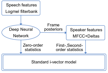
Figure 4: DNN-UBM/i-vector (from [12]). The posteriors are produced from the DNN acoustic model of an automatic speech recognition (ASR) system that is trained with, e.g. Logmel filterbank features. On the contrary, the sufficient statistics are computed from a speaker verification (SV) system that is trained with, e.g. MFCC which is not necessarily the same as the features for ASR. That is to say, one does not have to find a feature that works well for both ASR and SV in this framework.

3.2 DNN-UBM/i-vector

From (4), (5), and (6), one can see that only the posteriors of speech frames are needed to collect sufficient statistics for producing the i-vectors. Thus, we can use any probabilistic models beyond GMM-UBM to produce the posteriors theoretically [12]. Motivated by this insight, [12] proposed the DNN-UBM/i-vector framework (Fig.4) which takes a DNN acoustic model trained for ASR, denoted as DNN-UBM, to generate the posterior probabilities instead of GMM-UBM.

Specifically, DNN-UBM uses a set of senones $\mathcal{Q}=\{Q_{c}|c=1,2,\cdots,C\}$, e.g., the tied-triphone states, to mimic the mixture components of the GMM-UBM. It first trains a DNN-based ASR acoustic model to align each training frame with a senone, and then generates the posterior probabilities of each frame over the senones from the softmax output layer of the DNN acoustic model. The posteriors can be directly applied to (4), (5) and (6) to extract the DNN-UBM based i-vector. Due to the strong representation ability of DNN over GMM, DNN-UBM/i-vector yields 30% relative equal error rate (EER) reduction over GMM/i-vector on the telephone condition of the 2012 NIST speaker recognition evaluation (SRE) [12]. Later on, the authors in [33, 39, 43] further analyzed the performance of the DNN-UBM/i-vector in microphone and noisy conditions.

A lot of further studies bloomed the DNN-UBM/i-vector related techniques. For example, [36, 41] proposed to use a single ASR-DNN for both the speaker and language recognition tasks simultaneously. Additionally, [38] employed a time delay deep neural network (TDNN), which was originally applied to speech recognition, to compute the posteriors. It achieved the state-of-the-art performance on the NIST SRE10 corpus at the time. As a third instance, [45] replaced the feedforward DNN by a long short-term memory (LSTM) recurrent neural network (RNN). The last but not all, [44] studied a number of open issues relating to performance, computational complexity, and applicability of different types of DNNs.

The advantage of the DNN acoustic model may be brought by its strong ability in modeling content-related phonetic states explicitly, which not only generates highly compact representation of data but also provides precise frame alignment. This advantage is particularly apparent in text-dependent speaker verification [40, 31, 34, 32, 35]. However, this comes at the cost of greatly increased computational complexity over the traditional GMM-UBM/i-vector systems [38, 51], since that a DNN usually has more parameters than GMM. In addition, the training of the DNN based acoustic model requires a large number of labeled training data.

To overcome the computational complexity, a supervised GMM-UBM was also investigated based on the DNN acoustic model [38]. In specific, a GMM is obtained by:

$$\begin{split}\gamma_{ct}^{(i)}=&p(c|\mathbf{\overline{y}}_{t}^{(i)})\\ \omega_{c}=&\sum_{i,t}\gamma_{ct}^{(i)}\\ \bm{\mu}_{c}=&\frac{\sum_{i,t}\gamma_{ct}^{(i)}\mathbf{y}_{t}^{(i)}}{\sum_{i,t}\gamma_{ct}^{(i)}}\\ \bm{\Sigma}_{c}=&\frac{\sum_{i,t}\gamma_{ct}^{(i)}\mathbf{y}_{t}^{(i)}(\mathbf{y}_{t}^{(i)})^{T}}{\sum_{i,t}\gamma_{ct}^{(i)}}-\bm{\mu}_{c}\bm{\mu}_{c}^{T}\\ \end{split}$$ (7)

where $\mathbf{\overline{y}}_{t}^{(i)}$ and $\mathbf{y}_{t}^{(i)}$ denote the acoustic features for ASR and speaker recognition respectively, and $p(c|\mathbf{\overline{y}}_{t}^{(i)})$ is the posterior probability corresponding to the $c$th senones. By this way, the supervised-GMM maintains the training computational complexity of the traditional unsupervised-GMM, with a 20% relative EER reduction on the NIST SRE10 corpus [38]. Similar idea was also studied in [12], though no performance improvement over the baseline is observed. Although the supervised-GMM reduces the training computational complexity, training the DNN acoustic model still needs a large amount of labeled training data.

3.3 DNN-BNF/i-vector

The fundamental idea of DNN-BNF/i-vector is to extract a compact feature from the bottleneck layer of a DNN as the input of the factor analysis, where the bottleneck layer is a special hidden layer of the DNN that has much less hidden units than the other hidden layers. In practice, DNN-BNF/i-vector has many variants, as we have summarized in Fig. 5. Like DNN-UBM/i-vector, the deep model in DNN-BNF/i-vector is mainly trained to discriminate senones [32, 39, 47, 48, 36, 41] or phonemes [49, 50].

The input of the factor analysis can be either the bottleneck feature (BNF) produced from the bottleneck layer, a concatenation of BNF with other acoustic feature [49, 50], or a post-processed feature by principal components analysis (PCA) or linear discriminant analysis (LDA) [49, 50]. One can find that no matter whether we apply BNF alone [41] or concatenate it with other acoustic features [39], DNN-BNF/i-vector can significantly outperform the conventional GMM/i-vector, which indicates the effectiveness of the framework [36].

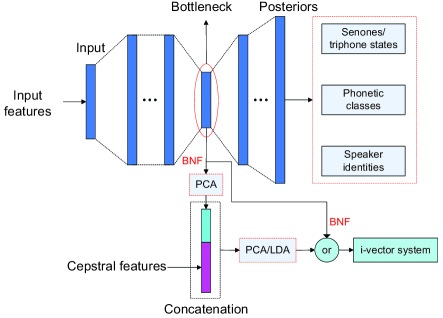
Figure 5: The DNN-BNF/i-vector framework. The framework is a summarization of related work. The term “PCA”, “LDA”, and “BNF” are short for principal components analysis, linear discriminant analysis, and bottleneck feature respectively.

However, it is unclear why a deep model trained to discriminate phonemes or senones can produce speaker-sensitive BNF. To address this issue, the authors of [47] assumed that speaker information is traded for dense phonetic information when the bottleneck layer moves toward the DNN output layer. Under this hypothesis, they experimentally analyzed the role of BNF by placing the bottleneck layer at different depths of the DNN. They found that, if the training and test conditions match, the closer the bottleneck layer is to the output layer, the better the performance is; otherwise, the bottleneck layer should be placed around the middle of the DNN. The authors of [48] explored whether weakening the accuracy of the acoustic model on speech recognition yields better BNF for speaker recognition. They analyzed the speaker recognition performance in different respects of the acoustic model, including under-trained DNN, different inputs, and different feature normalization strategies. Results indicate that high speech recognition performance in terms of phonetic accuracy does not necessarily imply increased speaker recognition accuracy. In addition, [46] proposed to take speaker identity as the training target, under the conjecture that this training target should be able to improve the robustness of the phonetic variability of BNF.

3.4 Discussion to the DNN/i-vector

Table 4: Comparison results between DNN/i-vector and GMM/i-vector. Each row denotes a comparison. The last three columns list the EER of the main models, the EER of the baselines, and the relative EER reductions, respectively. The results across rows are not comparable, since they are collected from different references, and their comparisons are not apple-to-apple comparisons.

Comparisons		Test dataset [condition]	EER
Main models	Baselines		Main	Baseline	Relative reduction
DNN-UBM [12]	GMM-UBM	NIST SRE12 C2	1.39%	1.81%	23%
DNN-UBM [12]	GMM-UBM	NIST SRE12 C5	1.92%	2.55%	25%
TDNN-UBM[38]	GMM-UBM	NIST SRE10 C5	1.20%	2.42%	50%
Sup-GMM-UBM[38]	GMM-UBM	NIST SRE10 C5	1.94%	2.42%	20%
BNF [36]	MFCC	In-domain DAC13	2.00%	2.71%	26%
BNF [36]	MFCC	Out-domain DAC13	2.79%	6.18%	55%

It is known that a major difference between DNN-UBM and GMM-UBM is that DNN-UBM is a discriminant model, while GMM-UBM is a generative one. DNN-UBM is more powerful than GMM-UBM in modeling a complicated data distribution [12, 38]. Moreover, the DNN acoustic model is trained to align each speech frame to its corresponding senone in a supervised fashion. Its output nodes have a clear physical explanation. It mines the pronunciation characteristics of speakers. On the contrary, GMM-UBM is trained by the expectation-maximum algorithm in an unsupervised manner. Its mixtures have no inherent meaning. Although DNN-UBM/i-vector needs labeled training data and heavier computation power than GMM-UBM, it does yield excellent performance. In addition, many corpora are also developed for the demand of training strong DNN, which will be reviewed in Section 11.

To demonstrate general performance differences of DNN/i-vector and GMM/i-vector, some carefully selected experimental results from literatures are listed in Table 4. Compared to the GMM-UBM/i-vector baseline, one can find that DNN-UBM/i-vector achieves more than 20% relative EER reduction over GMM-UBM/i-vector. In addition, the supervised GMM-UBM in (7) can also get 20% relative improvement according to the fourth row. Finally, from the last two rows, one can see that, when taking DNN-BNF and MFCC as the input features of the GMM-UBM/i-vector respectively, the former achieves better performance than the latter.

It should be note that, as far as we know, different test conditions may yield slightly different conclusions from those in Table 4. However, to our knowledge, the results in the table can be a representative of the research trend.

4 Speaker feature extraction with deep embedding

In this section, we first introduce two representative deep embeddings—d-vector and x-vector in Section 4.1 with some discussions in Section 4.2, and then identify their key components in Section 4.3, which provide a taxonomy to existing algorithms.

4.1 Two seminal work of deep embeddings

4.1.1 Frame-level embedding — d-vector

D-vector is one of the earliest DNN-based embeddings [13]. The core idea of d-vector is to assign the ground-truth speaker identity of a training utterance as the labels of the training frames belonging to the utterance in the training stage, which transforms the model training as a classification problem. As shown in Fig. 6, d-vector expands each training frame with its context, and employs a maxout DNN to classify the frames of a training utterance to the speaker identity of the utterance, where the DNN takes softmax as the output layer to minimize the cross-entropy loss between the ground-truth labels of the frames and the network output.

In the test stage, d-vector takes the output activation of each frame from the last hidden layer of the DNN as the deep embedding feature of the frame, and averages the deep embedding features of all frames of an utterance as a new compact representation of the utterance, named d-vector. An underlying hypothesis of d-vector is that the compact representation space produced from a development set may generalize well to unseen speakers in the test stage.

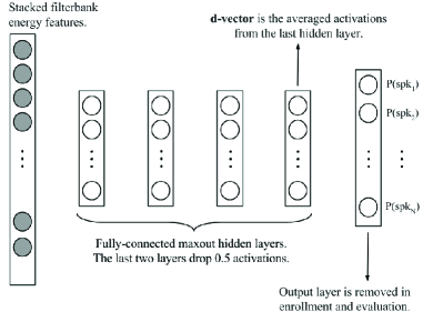
Figure 6: Diagram of the d-vector framework (from [13]).

4.1.2 Segment-level embedding — x-vector

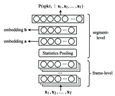
Figure 7: Diagram of the DNN model for extracting x-vectors (from [51]). Note that segment-level embeddings (e.g., $\mathbf{a}$ or $\mathbf{b}$) can be extracted from any layer of the network after the statistics pooling layer [51]. [14] where the name “x-vector” comes from uses the embedding a as the speaker feature.

X-vector [51, 14] is an important evolution of d-vector that evolves speaker recognition from frame-by-frame speaker labels to utterance-level speaker labels with an aggregation process. The network structure of x-vector is shown in Fig. 7. It first extracts frame-level embeddings of speech frames by time-delay layers, then concatenates the mean and standard deviation of the frame-level embeddings of an utterance as a segment-level (a.k.a., utterance-level) feature by a statistical pooling layer, and finally classifies the segment-level feature to its speaker by a standard feedforward network. The time-delay layers, statistical pooling layer, and feedforward network are jointly trained. X-vector is defined as the segment-level speaker embedding produced from the second to last hidden layer of the feedforward network, i.e. the variable $\mathbf{a}$ in Fig. 7.

The authors in [14] found that data augmentation is important in improving the performance of x-vector. We will introduce the data augmentation techniques in Section 10.3.

4.2 Discussion to the speaker embedding

Table 5: Characteristics of different speaker embeddings and their favorite back-ends.

Model name	Type	Training strategy	Label for model training	Back-end name	Label for back-end training
GMM-UBM/i-vector	Generative/Generative	Unsupervised/Unsupervised	✗/ ✗	PLDA	Speaker identity
DNN-UBM/i-vector	Discriminative/Generative	Supervised /Unsupervised	Phonetic labels/✗	PLDA	Speaker identity
DNN-BNF/i-vector	Discriminative/Generative	Supervised/Unsupervised	Phonetic labels /✗	PLDA	Speaker identity
D-vector	Discriminative	Supervised	Speaker identity	Cosine	✗
X-vector	Discriminative	Supervised	Speaker identity	PLDA	Speaker identity

Similar to the i-vector, the d-vector and x-vector are also a kind of speaker embedding, which discriminatively embeds speakers into a vector space by using DNNs. We call this type of speaker embedding as deep speaker embedding, or deep embedding for short. The main characteristics between different speaker embeddings are summarized in Table 5. Compared to the traditional GMM-UBM/i-vector, the deep embedding is a discriminant model and trained in a supervised fashion. Compared to DNN-UBM, its training data does not need phonetic-level labels. Therefore, the training of the deep embedding is much simpler than that of DNN-UBM and DNN-BNF. In addition, the deep embedding is a new framework, while DNN-UBM/i-vector and DNN-BNF/i-vector are hybrid ones.

Table 6: Selected results on deep embedding in literature. Each row represents a comparison. The results across rows are not comparable.

Comparison methods		Test dataset [condition]	EER
Deep embedding	Baseline		Deep embedding	Baseline	Relative reduction
d-vector [13]	GMM-UBM/i-vector	Google data	4.54%	2.83%	-37%
d-vector+i-vector [13]	GMM-UBM/i-vector	Google data [clean , noisy]	—–	—–	[14% , 25%]
embedding a+b (in Fig.7) [51]	GMM-UBM/i-vector	NIST SRE10 [10s-10s , 60s ]	[7.9% , 2.9%]	[11.0% , 2.3% ]	[28% , -21% ]
embedding a+b (in Fig.7) [51]	GMM-UBM/i-vector	NIST SRE16 [Cantonese , Tagalog ]	[6.5% , 16.3% ]	[8.3% , 17.6% ]	[22% , 7%]
x-vector (embedding a) [14]	GMM-UBM/i-vector	SITW Core [ PLDA and extractor aug. , Incl. VoxCeleb]	[ 6.00% , 4.16% ]	[ 8.04% , 7.45%]	[25%, 44%]
x-vector (embedding a) [14]	GMM-UBM/i-vector	SRE16 Cantonese [ PLDA and extractor aug. , Incl. VoxCeleb]	[ 5.86%, 5.71% ]	[ 8.95% , 9.23%]	[ 34%, 38%]

Some experimental results on deep embedding are listed in Table 6. From the table, one can find that, the d-vector alone yields higher EER than the i-vector. When fusing the d-vector and i-vector, the combined system achieves 14% and 25% relative EER reduction in clean and noisy test conditions respectively over the i-vector. The “embedding a+b” model, which is the predecessor of the x-vector, achieves lower EER than the GMM-UBM/i-vector baseline on the 10-second short utterances of NIST SRE10, and higher EER than the latter on the 60-second long utterances of NIST SRE10. With enlarged training data and data augmentation, the x-vector achieves significant performance improvement over the GMM-UBM/i-vector.

Fig. 8 shows the number of the related papers. We observe the following phenomena. First, the d-vector and DNN-UBM/i-vector was proposed both in 2014, where the former achieved better performance at the time. Second, the research on DNN/i-vector was mainly conducted in the first few years after its appearance, and then became less studied. Third, the research on deep embedding becomes bloom along with its performance improvement after that the x-vector achieved the state-of-the-art performance. At present, the deep embedding is the trend of speaker recognition, which has been developed in several aspects as summarized in the following subsection.

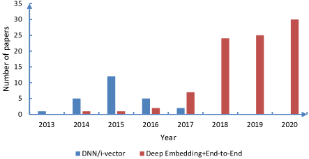
Figure 8: Statistics of the published papers on DNN/i-vector and deep embedding cited by this article.

4.3 Four key components of deep embedding

Motivated by the seminal work d-vector and x-vector, many deep embedding techniques were proposed, most of which are composed of four key components—network input, network structure, temporal pooling, and training objective. These components include but not limited to the following contents:

• Network inputs and structures: The network input can be categorized into two classes—raw wave signals in time domain and acoustic features in time-frequency domain, including spectrogram, Mel-filterbanks (f-bank), and MFCC. The network structure is diverse, which is rooted essentially at DNN, RNN/LSTM, and CNN. Because the network input and structure were jointly designed case by case in practice, we will jointly summarize them in Section 5.

• Temporal pooling: Temporal pooling represents the transition layer of a neural network that transforms frame-level embedding features to utterance-level embedding features. The temporal pooling strategies consist of two classes—statistical pooling and learning based pooling. We will introduce them in Section 6.

• Objective functions: Objective functions affect the effectiveness of speaker recognition much. Both d-vector and x-vector adopt softmax as the output layer and take the cross-entropy minimization as the objective function, which may not be optimal. Recently, many objectives were designed to further improve the performance. We will survey the objective functions in Section 7.

5 Deep embedding: network structures and inputs

Table 7: A brief summary of the inputs and neural network structures in deep speaker feature extraction.

Inputs	CNN	LSTM	Hybrid structures
Wave	Others [52, 53].	——	CNN-LSTM [54, 55]; CNN-GRU [56, 57].
Spectrogram	ResNet [58, 59, 60, 61]; VGGNet [15, 24]; Inception-resnet-v1 [62, 63].	——	CNN-GRU [64]
F-bank	TDNN [14, 65, 66, 67]; ResNet [68, 69, 70, 71]; VGGNet [72]; Inception-resnet-v1 [63, 73, 74]; Others [75, 76].	[77, 78, 79].	BLSTM-ResNet [80], TDNN-LSTM [81]
MFCC	TDNN [82, 51, 83, 84, 85, 86, 87, 88, 67, 89, 90, 91]; ResNet [92]; Others [93, 94].	——	TDNN-LSTM [95]

Although deep neural networks can be divided roughly into DNN, CNN, and RNN/LSTM structures, the network structure and input for speaker recognition are quite flexible. Each component of a network has many candidates. For example, the hidden layer of a neural network may be a standard convolutional layer [72], a dilated convolution layer [93], a LSTM layer [54], a gated recurrent unit (GRU) layer [56], a multi-head attention layer, a fully-connected layer, and even a combination of these different layers [54, 56], etc. The activation functions can be Sigmoid, Rectified Linear Unit (ReLU), Leaky ReLU, or Parametric Rectified Linear Unit (PReLU) etc. Besides, the topology of a network and connection mode between layers are all variables. Even the number of layers and number of hidden units at a layer can also affect the performance. To prevent enumerating the networks case by case, here we first review some commonly used networks for the speaker feature extraction, and then briefly review their inputs.

Time delay neural network (TDNN) [51]: TDNN takes a one-dimensional convolution structure along the time axis as a feature extractor [96]. It is adopted by the well known x-vector, as shown in Fig. 7. Due to the success of the x-vector [14, 82], TDNN becomes one of the most popular structures for speaker recognition. For example, [83] introduced phonetic information to the TDNN architecture based embedding extractor. [97] trained a TDNN embedding extractor without speaker labels via self-supervised training. [65, 66] explored the effectiveness of the orthogonality regularization by TDNN. Generally, TDNN has been frequently used as a framework to study other key components of the deep embedding models, such as the temporal pooling layers [84, 85] and objective functions [86, 87, 88].

The TDNN structure has also been intensively improved. For instance, an extended TDNN architecture (E-TDNN) was introduced in [82], which greatly outperforms the x-vector baseline [14]. It adopts a slightly wider temporal context than TDNN, and interleaves affine layers in between the convolutional layers [98]. [99] developed a factorized TDNN (F-TDNN) to reduce the number of parameters. It factorizes the weight matrix of each TDNN layer into the product of two low-rank matrices. It further constrains the first low-rank matrix to be semi-orthogonal under the assumption that the semi-orthogonal constraint prevents information loss. The application of F-TDNN to deep embedding was also investigated [89, 98, 100]. Some other parameter reduction works can be found in [101, 102]. Recently, [90] integrated TDNN with statistics pooling at each layer for compensating the variation of temporal context in the frame-level transforms. Similarly, [81, 95] inserted LSTM layers into TDNN to capture the temporal information for remedying the weakness of TDNN whose time delay layers focus on local patterns only. [91] alleviated the mismatch problem between training and evaluation by incorporating Bayesian neural networks into TDNN.

Residual networks (ResNet) [103]: it is another popular structure in speaker embedding. Its trunk architecture is a 2-dimensional CNN with convolutions in both the time and frequency domains. Some work directly used the standard ResNet as their speaker feature extractors [68, 58, 59, 69]. Some other work employed ResNet as a backbone and modified it for specific purposes or applications [60, 92, 80, 61, 70, 71]. For example, to reduce the number of parameters, [60] modified the standard ResNet-34 to a thin ResNet by cutting down the number of channels in each residual block. The authors in [80] combined bi-directional LSTM (BLSTM) and ResNet into a unified architecture, where the BLSTM is used to model long temporal contexts. The authors in [92] incorporated a so-called “squeeze-and-excitation” block into ResNet.

Raw wave neural networks [52, 53, 54, 55, 56, 57, 104, 105]: some work takes raw waves in the time domain as the input, which aims to extract learnable acoustic features instead of handcrafted features. For example, [52] applied CNN to capture raw speech signal. The experimental results indicate that the filters of the first convolution layer give emphasis to speaker information in low frequency regions. The authors in [53] believed that the first layer is critical for the waveform-based CNNs, since it not only deals with high-dimensional inputs, but suffers more from the gradient vanishing problem than the other layers. Therefore, they proposed a SincNet architecture based on parametrized sinc functions, where only low and high cutoff frequencies of band-pass filters are learned from data [53]. In [55], the authors thought that the difficulty of processing raw audio signals by DNN is mainly caused by the fluctuating scales of the signals. To stabilize the scales, they employed a convolutional layer, named pre-emphasis layer, to mimic the well-known signal pre-emphasis technique $p(t)=s(t)-\alpha s(t-1)$. They also made several improvements to the original raw wave network [56, 57, 104] which results in excellent performance. [105] designed a Wav2Spk architecture to learn speaker embeddings from waveforms, where the traditional MFCC extraction, voice activity detection, and cepstral mean and variance normalization are replaced by a feature encoder, a temporal gating unit and an instance normalization scheme respectively. Wav2Spk performs better than the convention x-vector network.

Other neural networks: in addition to TDNN and ResNet, many other well-known neural network architectures have also been applied to speaker recognition, including VGGNet [72, 24, 15], Inception-resnet-v1 [62, 63, 73, 74], BERT [106], and Transformer [107]. Besides, recurrent neural networks, such as LSTM and gated recurrent units, are often used for text-dependent speaker verification [77, 78, 79]. The CNN models can also be improved by inserting LSTM or gated recurrent units into the backbone networks [54, 55, 56, 57, 64, 80, 81, 95]. Finally, apart from the above handcrafted neural architectures, neural architecture search was also recently applied to speaker recognition [108, 109].

Neural network inputs: Table 7 provides a summary to the common inputs and neural networks for the deep embedding based speaker feature extraction. From the table, one can see that CNN-based neural networks and f-bank/MFCC acoustic features are becoming popular, while some 2-dimensional convolution structures, e.g. ResNet, use spectrogram as the input feature. In addition to the above common inputs, such as MFCC, spectrum and mel-filterbanks, [110] recently presented an extensive re-assessment of 14 acoustic feature extractors. They found that the acoustic features equipped with the techniques of spectral centroids, group delay function, and integrated noise suppression provide promising alternatives to MFCC.

5.1 Discussion to the networks

Table 8: Selected examples of the effect of neural network structures on performance (from [111]).

Comparison methods		Test dataset [condition]	EER
Main models	Baselines		Main	Baseline	Relative reduction
E-TDNN(10M)	TDNN(8.5M)	SITW EVAL CORE (16 kHz systems)	2.74%	3.40%	19%
F-TDNN(9M)	TDNN(8.5M)	SITW EVAL CORE (16 kHz systems)	2.39%	3.40%	30%
F-TDNN(17M)	TDNN(8.5M)	SITW EVAL CORE (16 kHz systems)	1.89%	3.40%	44%
ResNet(8M)	TDNN(8.5M)	SITW EVAL CORE (16 kHz systems)	3.01%	3.40%	11%

The network structure plays a key role on performance. For example, as shown in Table 8, E-TDNN and F-TDNN significantly reduced EER on the SITW dataset [16], where F-TDNN achieves more than 40% relative EER reduction over the original TDNN. Although this promotion is not consistent across all datasets [111], it demonstrates the importance of the network structure on performance.

For the acoustic features, the delta and double-delta features are helpful in statistical model based speaker recognition, e.g. the GMM-UBM/i-vector. However, they are not very effective in convolution and time-delay neural networks. This may be caused by that, the statistical model needs the delta and double-delta operations to capture the time dependency between frames, while the neural networks are able to achieve this goal intrinsically.

Although the deep embedding networks have achieved a great success, in our view, the following aspects can be further studied. First, the raw wave networks did not attract much attention. The mainstream of speaker recognition still adopts handcrafted features, which may lose useful information, e.g. the phase information, and finally may result in suboptimal performance as what we have observed in speech separation. Second, the model size and inference efficiency, which is important for the devices with limited computation source, e.g. edge or mobile devices, have not been fully studied. The topic was just recently investigated in [107, 102, 112].

6 Deep embedding: Temporal pooling layers

As shown in Fig. 7, the temporal pooling layer is a bridge between the frame-level and utterance-level hidden layers. Given a speech segment, we assume that the input and output of the temporal pooling layer are $\mathcal{H}=\{\mathbf{h}_{t}\in\mathbb{R}^{d_{2}}|t=1,2,\cdots,T\}$ and $\mathbf{u}$, respectively, where $\mathbf{h}_{t}$ denotes the $t$th frame-level speaker feature produced from the frame-level hidden layers. In this section, we introduce a number of temporal pooling functions.

6.1 Average pooling

Average pooling [62, 24, 69, 73] is the most common pooling function:

$$\mathbf{u}=\frac{1}{T}\sum_{t=1}^{T}\mathbf{h}_{t}$$ (8)

6.2 Statistics pooling

Statistics pooling [51, 14] calculates both the statistic mean $\mathbf{m}$ and standard deviation $\mathbf{d}$ of $\mathcal{H}$:

$$\mathbf{m}=\frac{1}{T}\sum_{t=1}^{T}\mathbf{h}_{t}$$ (9)

$$\mathbf{d}=\sqrt{\frac{1}{T}\sum_{t=1}^{T}\mathbf{h}_{t}\odot\mathbf{h}_{t}-\mathbf{m}\odot\mathbf{m}}\\$$ (10)

where $\odot$ denotes the Hadamard product. The output of the statistics pooling layer is a concatenation of $\mathbf{m}$ and $\mathbf{d}$, i.e. $\mathbf{u}=[\mathbf{m}^{T},\mathbf{d}^{T}]^{T}$.

6.3 Self-attention-based pooling

Obviously, (8), (9), and (10) assume that all elements of $\mathcal{H}$ contribute equally to $\mathbf{u}$. However, the assumption may not be true, since that the frames may not provide equal speaker-discriminative information. To address this issue, many works applied self attention mechanisms for weighted statistics pooling layers. Specifically, the attention can be broadly interpreted as a vector of importance weights, which allows a neural network to focus on a specific portion of its input. Further more, the self attention computes attentive weights within a single sequence.

In the following two subsections, we first present a general self attention framework which produces weighted means and standard deviations of the input from a self-attentive scoring function in Section 6.3.1, and then list a number of specific self-attention-based pooling methods under the framework in Section 6.3.2.

6.3.1 A self attention pooling framework

Without loss of generality, self-attentive scoring is defined as:

$$\big{\{}f_{\rm Att}^{(k)}(\cdot)|k=1,2,\cdots,K\big{\}}$$ (11)

where $f_{\rm Att}^{(k)}(\cdot)$ is usually referred as one-head, and $K$ is the total number of heads. If $K\geq 2$, the self attention mechanism is usually called multi-head self attention which allows the model to jointly attend to information from different representation subspaces [113]; otherwise, it degenerates into a single-head one. Although $f_{\rm Att}^{(k)}(\cdot)$ has many different implementations, many of the implementations share similar forms with the structured self-attentive function [114] which obtains the importance weights by:

$$f_{\rm Att}^{(k)}(\mathbf{h}_{t})=\mathbf{v}^{(k)^{T}}{\rm tanh}(\mathbf{W}^{(k)}\mathbf{h}_{t}+\mathbf{g}^{(k)})+b^{(k)},\quad k=1,2,\cdots,K$$ (12)

where $\mathbf{W}^{(k)}\in\mathbb{R}^{d_{3}\times d_{2}}$, $\mathbf{g}^{(k)}\in\mathbb{R}^{d_{3}}$, $\mathbf{v}^{(k)}\in\mathbb{R}^{d_{3}}$ and $b^{(k)}\in\mathbb{R}$ are learnable parameters of the $k$th scoring function. Suppose $s_{t}^{(k)}=f_{\rm Att}^{(k)}(\mathbf{h}_{t})$, $\quad k=1,2,\cdots,K$, then the importance weights for the frame-level feature $\mathbf{h}_{t}$ are obtained by normalizing $s_{t}^{(k)}$ with a softmax function:

$$\alpha_{t}^{(k)}=\frac{{\rm exp}\big{(}s_{t}^{(k)}\big{)}}{\sum_{t^{\prime}}^{T}{\rm exp}\big{(}s_{t^{\prime}}^{(k)}\big{)}},\quad k=1,2,\cdots,K$$ (13)

where the normalization guarantees that the weights satisfy $0\leq\alpha_{t}^{(k)}\leq 1$ and $\sum_{t=1}^{T}\alpha_{t}^{(k)}=1$. Finally, the weighted mean and standard deviation produced from the $k$th self-attentive scoring function can be derived as follows:

$$\widetilde{\mathbf{m}}^{(k)}=\sum_{t=1}^{T}\alpha_{t}^{(k)}\mathbf{h}_{t},\quad k=1,2,\cdots,K$$ (14)

$$\widetilde{\mathbf{d}}^{(k)}=\sqrt{\sum_{t=1}^{T}\alpha_{t}^{(k)}\mathbf{h}_{t}\odot\mathbf{h}_{t}-\mathbf{\widetilde{m}}^{(k)}\odot\mathbf{\widetilde{m}}^{(k)}},\quad k=1,2,\cdots,K$$ (15)

Finally, $\widetilde{\mathbf{m}}^{(k)}$ and $\widetilde{\mathbf{d}}^{(k)}$ are used to calculate an utterance-level representation as described in the following subsection.

6.3.2 Attention pooling methods

Under the above attention framework, this subsection categorizes existing self-attention based pooling layers into the following six classes, where all methods take (12) as the self-attentive scoring function and take (13) as the normalization function, unless otherwise stated.

• Single-head attentive average pooling [72, 115, 77]: [72] takes a fully-connected layer as $f_{\rm Att}(\cdot)$. [115] adopts the cosine function to compute attention scores:

  $$s_{t}=f_{\rm Att}(\mathbf{h}_{t},\mathbf{r})=\frac{\mathbf{h}_{t}^{T}\mathbf{r}}{\|\mathbf{h}_{t}\|_{2}\|\mathbf{r}\|_{2}}$$ (16)

  where $\mathbf{r}$ is a nonlinearly transformed i-vector from the same utterance as $\mathbf{h}$. Obviously, the attention weights in (16) are determined by both the frame-level $\mathbf{h}_{t}$ and the utterance-level information $\mathbf{r}$. In [77], several attentive functions similar to (12) are investigated.

  The output of the single-head attentive average pooling is set to the weighted mean:

  $$\mathbf{u}=\mathbf{\widetilde{m}}^{(1)}.$$ (17)

• Single-head attentive statistics pooling [85]: It uses a single-head attention function, i.e. $K=1$. Its output is a concatenation of both the weighted mean and weighted standard deviation:

  $$\mathbf{u}=[\widetilde{\mathbf{m}}^{(1)^{T}},\widetilde{\mathbf{d}}^{(1)^{T}}]^{T}.$$ (18)

• Single-head Baum-Welch statistics attention mechanism based statistics pooling [116]: To overcome the weakness of (12) which cannot fully mine the inner relationship between an utterance and its frames, [116] integrated the Baum-Welch statistics into the attention mechanism:

  $$s_{t}=\mathbf{v}^{T}{\rm tanh}(\mathbf{K}\mathbf{q}_{t}+\mathbf{g})$$ (19)

  where $\mathbf{K}$ is named the key matrix and $\mathbf{q}_{t}$ is a query vector calculated by:

  $$\mathbf{q}_{t}=f(\mathbf{h}_{t}^{(-1)})$$ (20)

  where $f(\cdot)$ is a nonlinear function, and $\mathbf{h}_{t}^{(-1)}$ denotes the output of a penultimate frame-level hidden layer. The key matrix $\mathbf{K}$ is calculated from the Baum-Welch statistics. Specifically, [116] first calculates the normalized first order statistics $\mathbf{f}_{c}$ from the $c$th component of a GMM-UBM model $\Omega$ (see (5)), and then conducts the following nonlinear transform:

  $$\mathbf{f}_{c}^{\prime}=\mathbf{V}_{2}{\rm tanh}(\mathbf{V}_{1}\mathbf{f}_{c}+\mathbf{g}),\quad\forall c=1,\ldots,C$$ (21)

  where $\mathbf{V}_{1}$, $\mathbf{V}_{2}$ and $\mathbf{g}$ are the parameters of DNN. Finally, it concatenates $\mathbf{F}^{\prime}=[\mathbf{f}_{1}^{\prime},\mathbf{f}_{2}^{\prime},\cdots,\mathbf{f}_{C}^{\prime}]$ and the trainable matrix $\mathbf{W}$ as the key matrix:

  $$\mathbf{K}=[\mathbf{F}^{\prime},\mathbf{W}]^{T}$$ (22)

  After obtaining $s_{t}$, $\mathbf{u}$ is obtained in the same way as (18).

• Global multi-head attentive average pooling: It first applies a $K$-head ($K\geq 2$) attention function to $\mathcal{H}$ by (12). Then, the attentive weights and weighted means are calculated by (13) and (14) respectively [68]. Finally, the output of the pooling layer $\mathbf{u}$ is the concatenation of the weighted means:

  $$\mathbf{u}=[\widetilde{\mathbf{m}}^{(1)^{T}},\widetilde{\mathbf{m}}^{(2)^{T}},\cdots,\widetilde{\mathbf{m}}^{(K)^{T}}]^{T}$$ (23)

  It can be seen that $\mathbf{u}\in\mathbb{R}^{Kd_{2}}$. Similar ideas can also be found in [84, 117]. [84] also added an additional penalty term into the objective function to enlarge the diversity between the heads.

• Sub-vectors based multi-head attentive average pooling [118]: It first splits $\mathbf{h}_{t}$ into $K$ ($K\geq 2$) non-overlapping homogeneous sub-vectors $\mathbf{h}_{t}=[\mathbf{h}_{t}^{(1)^{T}},\mathbf{h}_{t}^{(2)^{T}},\cdots,\mathbf{h}_{t}^{(K)^{T}}]^{T}$, where $\mathbf{h}_{t}^{(k)}\in\mathbb{R}^{d_{2}/K}$. Then, it applies single-head attention to each of the sub-vectors $\mathcal{H}^{(k)}=\{\mathbf{h}_{t}^{(k)}\in\mathbb{R}^{d_{2}/K}|t=1,2,\cdots,T\}$. Finally, it obtains the sub-pooling outputs by:

  $$\mathbf{u}^{(k)}=\sum_{t=1}^{T}\alpha_{t}^{(k)}\mathbf{h}_{t}^{(k)},\quad k=1,2,\cdots,K$$ (24)

  It can be seen that $\mathbf{u}^{(k)}\in\mathbb{R}^{d_{2}/K}$. The output of the pooling layer is a concatenation of the sub-pooling outputs:

  $$\mathbf{u}=[\mathbf{u}^{(1)^{T}},\mathbf{u}^{(2)^{T}},\cdots,\mathbf{u}^{(K)^{T}}]^{T}.$$ (25)

• Multi-resolution multi-head attentive average pooling [68]: Because the speaker characteristics are obtained through the aggregation of the attentive weights reweighted frame-level features, [68] proposed to control the resolution of the attentive weights with a temperature parameter. They modify the softmax function as:

  $$\alpha_{t}=\frac{{\rm exp}(s_{t}/E)}{\sum_{t^{\prime}=1}^{T}{\rm exp}(s_{t^{\prime}}/E)}$$ (26)

  where $E$ is the temperature parameter. It is obvious that increasing $E$ makes the distribution of $\alpha_{t}$ less sharp, i.e. lower resolution. By incorporating the above intuition, the weighting equation (13) is changed to:

  $$\alpha_{t}^{(k)}=\frac{{\rm exp}\big{(}s_{t}^{(k)}/E_{k}\big{)}}{\sum_{t^{\prime}}^{T}{\rm exp}\big{(}s_{t^{\prime}}^{(k)}/E_{k}\big{)}}$$ (27)

  where $E_{k}\geq 1$ is a temperature hyperparameter of the $k$th head. Finally, the output $\mathbf{u}$ is calculated in a similar way with that of the global multi-head attentive average pooling except that $\alpha_{t}^{(k)}$ is replaced by (27).

It is clear that the above attentive pooling methods all employ scalar attention weights for each frame-level vector. [119] further proposed a vector-based attentive pooling method, which adopts vectorial attention weights for each frame-level vector.

6.4 NetVLAD $\&$ GhostVLAD pooling

In [60], the authors applied a dictionary-based NetVLAD layer to aggregate features across time, which can be intuitively regarded as trainable discriminative clustering: every frame-level descriptor will be softly assigned to different clusters, making the residuals encoded as the output feature [60].

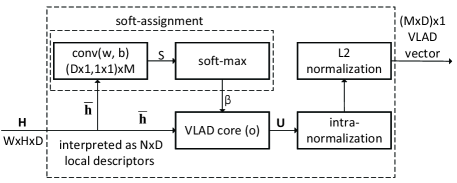
Figure 9: Diagram of the NetVLAD pooling layer (from [120]).

Specifically, as shown in Fig. 9, suppose that the input of the NetVLAD layer is a three-dimensional tensor $\mathbf{H}^{(W\times H)\times D}$, where $W$, $H$ and $D$ depend on the speech length, the dimensions of the spectrum frequency bins, and the number of convolution kernels respectively. By only retaining the third dimension, $\mathbf{H}$ can be converted to $N$ one-dimensional tensors, i.e. $\overline{\mathcal{H}}=\{\overline{\mathbf{h}}_{n}\in\mathbb{R}^{D}|n=1,2,\cdots,N\}$ where $N=W\times H$. As shown in Fig. 9, the NetVLAD pooling layer consists of the following four steps [120]:

1. Calculate a matrix $\mathbf{U}\in\mathbb{R}^{D\times M}$ from $\overline{\mathcal{H}}$ by:

   $$\mathbf{U}(:,m)=\sum_{n=1}^{N}\beta_{m}(\mathbf{\overline{h}}_{n})(\mathbf{\overline{h}}_{n}-\mathbf{o}_{m})$$ (28)

   where $M$ is the number of the chosen clusters $\mathcal{O}=\{\mathbf{o}_{m}\in\mathbb{R}^{D}|m=1,2,\cdots,M\}$, and $\beta_{m}(\mathbf{\overline{h}}_{n})$ is an assignment weight calculated by:

   $$\beta_{m}(\mathbf{\overline{h}}_{n})=\frac{{\rm exp}\big{(}\mathbf{w}_{m}^{T}\mathbf{\overline{h}}_{n}+b_{m}\big{)}}{\sum_{m^{\prime}=1}^{M}{\rm exp}\big{(}\mathbf{w}_{m^{\prime}}^{T}\mathbf{\overline{h}}_{n}+b_{m^{\prime}}\big{)}}$$ (29)

   with $\{\mathbf{w}_{m}\}$, $\{b_{m}\}$ and $\{\mathbf{o}_{m}\}$ as the parameters of the network.

2. Normalize $\mathbf{U}$ by $\ell_{2}$-norm column-wisely. This step is termed as the intra-normalization.

3. Convert the normalized $\mathbf{U}$ into a vector:

   $$\mathbf{u}=[\mathbf{U}(:,1)^{T},\mathbf{U}(:,2)^{T},\cdots,\mathbf{U}(:,M)^{T}]^{T}$$ (30)

4. Normalize $\mathbf{u}$ by $\ell_{2}$-norm to generate an $M\times D$ dimensional output vector. This step is termed as the $\ell_{2}$-normalization.

In addition, [60] also applied a variant of NetVLAD, named GhostVLAD. The main difference between them is that some of the clusters in the GhostVLAD layer, named “ghost clusters”, are not included in the final concatenation, and hence do not contribute to the final representation. When aggregating the frame-level features, the contribution of the noisy and undesirable sections of a speech segment to the normal VLAD clusters will be effectively down-weighted, since that larger weights are assigned to the “ghost cluster”. See [121] for the details.

6.5 Learnable dictionary encoding pooling

Motivated by GMM-UBM, [122] proposed a learnable dictionary encoding (LDE) pooling layer which models the distribution of the frame-level features $\mathcal{H}$ by a dictionary. The dictionary learns a set of dictionary component centers $\mathcal{\overline{O}}=\big{\{}\mathbf{\overline{o}}_{m}\in\mathbb{R}^{d_{2}}|m=1,2,\cdots,M\big{\}}$, and assigns weights to the frame-level features by:

$$\overline{\beta}_{tm}=\frac{{\rm exp}(-\tau_{m}||\mathbf{h}_{t}-\mathbf{\overline{o}}_{m}||^{2})}{\sum_{m^{\prime}=1}^{M}{\rm exp}(-\tau_{m^{\prime}}||\mathbf{h}_{t}-\mathbf{\overline{o}}_{m^{\prime}}||^{2})}$$ (31)

where the smoothing factor $\tau_{m}$ for each dictionary center $\mathbf{\overline{o}}_{m}$ is learnable. The aggregated output of the pooling layer with respect to the center $\mathbf{\overline{o}}_{m}$ is:

$$\mathbf{u}_{m}=\frac{\sum_{t=1}^{T}\overline{\beta}_{tm}(\mathbf{h}_{t}-\overline{\mathbf{o}}_{m})}{\sum_{t=1}^{T}\overline{\beta}_{tm}}$$ (32)

In order to facilitate the derivation, (32) is simplified to:

$$\mathbf{u}_{m}=\frac{\sum_{t=1}^{T}\overline{\beta}_{tm}(\mathbf{h}_{t}-\overline{\mathbf{o}}_{m})}{T}$$ (33)

Finally, the output of the pooling layer is $\mathbf{u}=[\mathbf{u}_{1}^{T},\mathbf{u}_{2}^{T},\cdots,\mathbf{u}_{M}^{T}]^{T}$.

6.6 Spatial pyramid pooling

In order to handle variable-length utterances, [63] incorporated a Spatial Pyramid Pooling operation into a CNN-based network, which can directly produce fixed-length feature vectors from variable-length utterances.

As shown in Fig. 10, the spatial pyramid pooling layer outputs a fixed length vector by first dividing the input feature maps into $1\times 1$, $2\times 2$, and $3\times 3$ small patches and then performing average pooling over these patches. An exceptional advantage of the spatial pyramid pooling layer is that it maintains spatial information of the last frame-level feature maps by making average pooling in each local small patches.

[123] further extracted embeddings from the divided small patches via a parameter-sharing LDE layer instead of applying the averaging pooling on them.

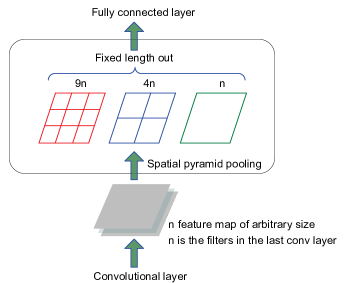
Figure 10: Spatial pyramid pooling (from [63]).

6.7 Other temporal pooling functions

There are many other successful pooling methods. For example, [93] proposed a cross-convolutional-layer pooling method to capture the first-order statistics for modelling long-term speaker characteristics. [124] reported a total variability model based pooling layer. [79] connected the last output of LSTM to the loss function for an utterance-level speaker representation. Apart from the single-scale aggregation methods in Sections 6.1 to 6.6 which generate the pooling output from the last frame-level layer, multiscale aggregation methods have also been proposed [81, 125, 126, 127, 128] which utilize multiscale features from different frame-level layers to generate the pooling output.

6.8 Discussion to the temporal pooling layers

Because temporal pooling layers behave fundamentally different in different datasets, network structures, or loss functions, it is difficult to conclude which one is the best. To our knowledge, temporal pooling functions with learnable parameters achieved better (at least competitive) results than the simple pooling layers such as the average pooling and statistical pooling in most cases, with a weakness of higher computational complexity than the latter. Some examples are listed in Table 9.

Table 9: Experimental results of different temporal pooling functions selected from literature. Each row represents a comparison. The results across rows are not comparable.

Comparison methods		Test dataset [condition]	EER
Main models	Baselines		Main	Baseline	Relative reduction
Attention[84]	Average	SRE16 Cantonese	5.81%	7.33%	21%
NetVLAD [60]	Average	VoxCeleb1 test set	3.57%	10.48%	66%
GhostVLAD [60]	Average	VoxCeleb1 test set	3.22%	10.48%	69%
LDE [111]	Statistics	SITW	2.50%	3.01%	17%

7 Deep embedding: Classification-based objective functions

The objective function largely determines the performance of a neural network. Deep-embedding-based speaker recognition systems usually adopt classification-based objective functions. Before reviewing the objective functions, we first summarize the deep-embedding-based speaker recognition as the following multi-class classification problem.

Let $\mathcal{X}=\{(\mathbf{x}_{n},l_{n})|n=1,2,\cdots,N\}$ denote the training samples in a mini-batch, where $\mathbf{x}_{n}\in\mathbb{R}^{d_{4}}$ represents the input of the last fully connected layer, $l_{n}\in\{1,2,\cdots,J\}$ is the class label of $\mathbf{x}_{n}$ with $J$ as the number of speakers in the training set, and $N$ is the batch size. In addition, $\mathbf{W}=[\mathbf{w}_{1},\mathbf{w}_{2},\cdots,\mathbf{w}_{J}]$ and $\mathbf{b}=[b_{1},b_{2},\cdots,b_{J}]$ denote the weight matrix and bias vector of the last fully connected layer respectively.

In this section, we comprehensively summarize the classification based objective functions. Without loss of generality, the “loss function”,“cost function” and “objective function” are equivalent in this article.

7.1 The variants of softmax loss

As shown in Section 4, both the d-vector and x-vector extractors take the minimum cross entropy as the objective function, and take softmax as the output layer. For short, we denote the objective function as the Softmax loss. For a multiclass classification problem, the cross-entropy error function over $\mathcal{X}$ can be calculated as:

$$L=-\frac{1}{N}\sum_{n=1}^{N}{\sum_{j=1}^{J}t_{nj}{\rm log}p_{nj}}$$ (34)

where $[t_{n1},t_{n2},\cdots,t_{nJ}]$ is a one-hot vector encoded from the label $l_{n}$, in other words, $t_{nj}$ equals to 1 if and only if sample $\mathbf{x}_{n}$ belongs to class $j$. $p_{nj}$ is the posterior probability of $\mathbf{x}_{n}$ belonging to class $j$. It is produced from neural networks with the following Softmax function:

$$p_{nj}=\frac{{\rm exp}{(\mathbf{w}_{j}^{T}\mathbf{x}_{n}+b_{j}})}{\sum_{j=1}^{J}{\rm exp}{(\mathbf{w}_{j}^{T}\mathbf{x}_{n}+b_{j}})}$$ (35)

Combining (34) and (35) derives an equivalent form of the Softmax loss:

$$\mathcal{L}_{\rm S}=-\frac{1}{N}\sum_{n=1}^{N}{\rm log}\frac{{\rm exp}{(\mathbf{w}_{l_{n}}^{T}\mathbf{x}_{n}+b_{l_{n}}})}{\sum_{j=1}^{J}{\rm exp}{(\mathbf{w}_{j}^{T}\mathbf{x}_{n}+b_{j}})}$$ (36)

Softmax loss is the most common objective function for deep embedding. However, from (36), one can see that Softmax loss is only good at maximizing the between-class distance, but does not have an explicit constraint on minimizing the within-class variance. Therefore, the performance of deep embedding has much room of improvement. Here we present some representative variants of Softmax loss as follows.

• Angular softmax (ASoftmax) loss [130, 131, 122]: Because the inner product between $\mathbf{w}_{j}$ and $\mathbf{x}_{n}$ in (36) can be rewritten as:

  $$\mathbf{w}_{j}^{T}\mathbf{x}_{n}=\|\mathbf{w}_{j}\|\,\|\mathbf{x}_{n}\|{\rm cos}(\theta_{j,n})$$ (37)

  where $\theta_{j,n}(0\leq\theta_{j,n}\leq\pi)$ denotes the angle between $\mathbf{w}_{j}$ and $\mathbf{x}_{n}$, Softmax loss can be rewritten as:

  $$\mathcal{L}_{\rm S}=-\frac{1}{N}\sum_{n=1}^{N}{\rm log}\frac{{\rm exp}{\big{(}\|\mathbf{w}_{l_{n}}\|\,\|\mathbf{x}_{n}\|{\rm cos}(\theta_{l_{n},n})+b_{l_{n}}}\big{)}}{\sum_{j=1}^{J}{\rm exp}{\big{(}\|\mathbf{w}_{j}\|\,\|\mathbf{x}_{n}\|{\rm cos}(\theta_{j,n})+b_{j}}\big{)}}$$ (38)

  If we further set the bias terms to zero, normalize the weights at the forward propagation stage, and add a margin to the angle:

  $$b_{j}=0,\quad\|\mathbf{w}_{j}\|=1,\quad\psi(\theta_{l_{n},n})=(-1)^{a}{\rm cos}(m_{1}\theta_{l_{n},n})-2a$$ (39)

  then, we explicitly constrain the learned features to have a small intra-speaker variation, where $m_{1}\geq 1$ is an integer margin hyperparameter, $\theta_{l_{n},n}\in[\frac{a\pi}{m_{1}},\frac{(a+1)\pi}{m_{1}}]$, and $a\in\{0,1,\cdots,m_{1}-1\}$. The intuition behind the angle function $\psi(\theta_{l_{n},n})$ is illustrated in Fig. 11. Then, we obtain ASoftmax loss as follows:

  $$\begin{split}&\mathcal{L}_{\rm AS}=\\ &-\frac{1}{N}\sum_{n=1}^{N}{\rm log}\frac{{\rm exp}{\big{(}\|\mathbf{x}_{n}\|\psi(\theta_{l_{n},n})})}{{\rm exp}{\big{(}\|\mathbf{x}_{n}\|\psi(\theta_{l_{n},n})})+\sum_{j=1,j\neq l_{n}}^{J}{\rm exp}{\big{(}\|\mathbf{x}_{n}\|{\rm cos}(\theta_{j,n})}\big{)}}\end{split}$$ (40)

  Note that, because $m_{1}$ is limited to a positive integer instead of a real number, the margin is not flexible enough.

  

  Figure 11: Illustration of the angle function of the ASoftmax loss. Obviously, the angle $\theta_{l_{n},n}$ in the training stage is in $[0,\pi]$. If we simply multiply an integer margin $m_{1}$ to $\theta_{l_{n},n}$, then the angle function $\psi_{1}(\cdot)$ is monotonic when $\theta_{l_{n},n}\in[0,\frac{\pi}{m_{1}}]$ only. Therefore, in practice, $\psi_{1}(\cdot)$ is generalized to $\psi_{2}(\cdot)$ to ensure that the angle function is monotonically decreasing when $\theta\in[0,\pi]$.

• Additive margin softmax (AMSoftmax) loss [60, 132, 58]: It is a revision of ASoftmax loss by replacing $\psi(\theta_{l_{n},n})$ in (40) with $({\rm cos}(\theta_{l_{n},n})-m_{2})$, and normalizing $\|\mathbf{x}_{n}\|=1$:

  $$\begin{split}&\mathcal{L}_{\rm AMS}=\\ &-\frac{1}{N}\sum_{n=1}^{N}{\rm log}\frac{{\rm exp}{\big{(}\tau({\rm cos}(\theta_{l_{n},n})-m_{2})}\big{)}}{{\rm exp}{\big{(}\tau({\rm cos}(\theta_{l_{n},n})-m_{2})\big{)}}+\sum_{j=1,j\neq l_{n}}^{J}{\rm exp}{\big{(}\tau({\rm cos}(\theta_{j,n})})\big{)}}\end{split}$$ (41)

  where $\tau$ is a scaling factor for preventing gradients too small during the training process [88]. In addition, [133] also proposed a dynamic-additive margin softmax, where $m_{2}$ is replaced by a dynamic margin for each training sample.

• Additive angular margin softmax (AAMSoftmax) [88, 134]: It replaces $({\rm cos}(\theta_{l_{n},n})-m_{2})$ in (41) by ${\rm cos}(\theta_{l_{n},n}+m_{3})$:

  $$\begin{split}&\mathcal{L}_{\rm AAMS}=\\ &-\frac{1}{N}\sum_{n=1}^{N}{\rm log}\frac{{\rm exp}{\big{(}\tau({\rm cos}(\theta_{l_{n},n}+m_{3}))}\big{)}}{{\rm exp}{\big{(}\tau({\rm cos}(\theta_{l_{n},n}+m_{3}))\big{)}}+\sum_{j=1,j\neq l_{n}}^{J}{\rm exp}{\big{(}\tau({\rm cos}(\theta_{j,n})})\big{)}}\end{split}$$ (42)

To further improve the convergence speed and accuracy, [135] recently proposed a parameter adaptation method which adapts the scaling factor $\tau$ and margin $m_{3}$ at each iteration.

Compared to Softmax, both ASoftmax, AMSoftmax, and AAMSoftmax benefit from the following two aspects: first, the learned features are angularly distributed, which matches with the cosine similarity scoring back-end; second, they introduce an angle, i.e. a cosine margin, to quantitatively control the decision boundary between training speakers for minimizing the within-class variance. More information can be found in [129, 136, 137, 138].

7.2 Regularization for Softmax loss and its variants

As illustrated in Section 7.1, the learned feature by the Softmax loss is not discriminative enough. To address this issue, an alterative way is to combine the Softmax loss with some regularizers [129]:

$$\mathcal{L}=\mathcal{L}_{\rm S}+\lambda\mathcal{L}_{\rm Regular}$$ (43)

where $\lambda$ is a hyperparameter for balancing the Softmax loss $\mathcal{L}_{\rm S}$ and the regularizer $\mathcal{L}_{\rm Regular}$. Besides, the regularizer is also applicable to other Softmax variants.

Because the embedding layer that produces the embedding speaker features is not always the last hidden layer, e.g. the x-vector in Fig.7, the regularizer was sometimes added to the embedding layer. For clarity, we define the output of the embedding layer as $\mathcal{E}=\{(\mathbf{e}_{n},l_{n})|n=1,2,\cdots,N\}$ , where $\mathbf{e}_{n}\in\mathbb{R}^{d_{5}}$. Here we introduce some regularizers as follows:

• Center loss [122, 73, 139]: It is a typical regularizer for Softmax loss. It explicitly minimizes the within-class variance by:

  $$\mathcal{L}_{\rm C}=\frac{1}{2}\sum_{n=1}^{N}\|\mathbf{e}_{n}-\mathbf{c}_{l_{n}}\|^{2}$$ (44)

  where $\mathbf{c}_{l_{n}}\in\mathbb{R}^{d_{5}}$ denotes the $l_{n}$th class center of the elements in $\mathcal{E}$. At each training iteration, the centers are updated as follows [73]:

  $$\mathbf{c}_{j}^{t+1}=\mathbf{c}_{j}^{t}-\epsilon\Delta\mathbf{c}_{j}^{t}$$ (45)

  $$\Delta\mathbf{c}_{j}=\frac{\sum_{n=1}^{N}\delta(l_{n}=j)\cdot(\mathbf{c}_{j}-\mathbf{e}_{n})}{1+\sum_{n=1}^{N}\delta(l_{n}=j)}$$ (46)

  where $\epsilon\in[0,1]$ controls the learning rate of the centers, the superscript “$t$” represents the number of iterations, and $\delta(\cdot)$ is an indicator function. If the condition of the indicator function, i.e. $l_{n}=j$, is satisfied, then $\delta=1$; otherwise, $\delta=0$.

  The center loss is usually combined with Softmax loss:

  $$\mathcal{L}=\mathcal{L}_{\rm S}+\lambda\mathcal{L}_{\rm C}$$ (47)

  See [140] for more information about the center loss.

• Ring loss [134]: It restricts $\|\mathbf{e}_{n}\|$ to be close to a target value $R$ for AMSoftmax loss:

  $$\mathcal{L}=\mathcal{L}_{\rm AMS}+\lambda\times\frac{1}{N}\sum_{n=1}^{N}(\|\mathbf{e}_{n}\|-R)^{2}$$ (48)

  where the target norm $R$ is optimized during the network training. Equation (48) essentially applies a normalization constraint to the features.

• Minimum hyperspherical energy criterion [134]: It enforces the weights of the output layer to distribute evenly on a hypersphere:

  $$\mathcal{L}=\mathcal{L}_{\rm AMS}+\frac{\lambda}{N(J-1)}\sum_{n=1}^{N}\sum_{j=1,j\neq l_{n}}^{J}h(\|\hat{\mathbf{w}}_{l_{n}}-\hat{\mathbf{w}}_{j}\|)$$ (49)

  where $\hat{\mathbf{w}}_{l_{n}}$ and $\hat{\mathbf{w}}_{j}$ are the $\ell_{2}$-normalized $\mathbf{w}_{l_{n}}$ and $\mathbf{w}_{j}$ respectively, and $h(z)=\frac{1}{z^{2}}$ is a decreasing function. Intuitively, the minimum hyperspherical energy based regularizer enlarges the inter-class separability.

• Gaussian prior [87]: To reduce information leak, [87] introduced a Gaussian prior to the output of the embedding layer, which results in the following objective function:

  $$\mathcal{L}=\mathcal{L}_{\rm S}+\lambda\sum_{j}\sum_{\mathbf{e}_{n}\in\varepsilon(j)}\|\mathbf{e}_{n}-\mathbf{w}_{j}\|$$ (50)

  where $\varepsilon(j)$ is the set of the utterances belonging to the $j$th speaker, $\mathbf{e}_{n}$ represents the x-vector, $\mathbf{w}_{j}$ represents the parameters of the last layer corresponding to the output unit of speaker $j$.

• Triplet loss [141]: Because Softmax loss does not explicitly reduce intra-class variance, triplet loss was introduced to directly bring samples from the same class closer than the samples from different classes. Formally, the triplet loss weighted Softmax loss is written as:

  $$\mathcal{L}=\lambda\mathcal{L}_{\rm S}+(1-\lambda)\mathcal{L}_{\rm Triplet}$$ (51)

  where $\mathcal{L}_{\rm Triplet}$ denotes the triplet loss, which will be introduced in Section 8.

There are also many other regularization approaches. For example, [58] added a Hilbert-Schmidt independence criterion based constraint to the embedding layer for regularizing AMSoftmax loss $\mathcal{L}_{\rm AMS}$. See [58] for the details.

7.3 Multi-task learning for deep embedding

Phonetic information is important in improving the performance of speaker recognition. As illustrated in Section 3, one way to incorporate phonetic information into the i-vector-based systems is to employ an ASR acoustic model, e.g. the DNN-UBM/i-vector or the DNN-BNF/i-vector. As for the deep-embedding-based speaker recognition, the phonetic information was usually incorporated by multi-task learning. For example, [142, 143] trained a deep embedding network to discriminate the speaker identity and text phrases simultaneously. The training objective is to minimize:

$${\rm CE}([\bm{l}_{1},\bm{l}_{2}],[\bm{l}_{1}^{\prime},\bm{l}_{2}^{\prime}])={\rm CE}_{1}(\bm{l}_{1},\bm{l}_{1}^{\prime})+{\rm CE}_{2}(\bm{l}_{2},\bm{l}_{2}^{\prime})$$ (52)

where ${\rm CE}_{1}$ and ${\rm CE}_{2}$ are two cross-entropy criteria for speaker and text phrase respectively. $\bm{l}_{1}$ and $\bm{l}_{2}$ indicate the true labels for speakers and text individually, and $\bm{l}_{1}^{\prime}$ and $\bm{l}_{2}^{\prime}$ are the two outputs of the network respectively. Some similar ideas can also be found in [144].

Although the text content may be a harmful source to text-independent speaker recognition, some positive results were observed with the multi-task learning. The authors in [83] added phonetic information to the frame-level layers of the x-vector extractor with an auxiliary ASR acoustic model by multi-task learning. The authors in [145] conjectured that the phonetic information is helpful for frame-level feature learning, however, it is useless in utterance-level speaker embeddings. They experimentally verified their assumptions by multitask learning and adversarial training, where the phonetic information was used as positive and negative effects respectively.

Besides the phonetic information mining, some multi-task learning approaches intend to improve the performance of the auxiliary and main tasks together. For example, [146] proposed a collaborative learning approach based on multi-task recurrent neural model to improve the performance of both speech and speaker recognition. [147] proposed a multitask DNN structure to denoise i-vectors and classify speakers simultaneously. Considering that the acoustic and speaker domains are complementary, [148] recently proposed a multi-task network that performs keyword spotting and speaker verification simultaneously to fully utilize the interrelated domain information.

7.4 Discussion to the classification-based loss functions

Because speaker verification is an open set recognition task, the deep embedding space produced from a training dataset with a limited number of speakers is required to generalize well to unseen test speakers. Therefore, it is the speaker discriminative ability of the embedding rather than the classification accuracy that is important, which accounts for the motivation why many classification-based loss functions are designed to minimize the within-class variance by adding a margin or a regularizer into the Softmax loss.

From the experimental results in literature, one can concluded that the design of loss functions is very important to performance. At present, nearly all stat-of-the-art deep embedding systems replaced the traditional Softmax by its variants, especially AMSoftmax and AAMSoftmax. In addition, the Softmax loss, its variants and regularizers are not mutually exclusive. For instance, the regularization terms (48) and (49) were originally added to AMSoftmax [134].

8 End-to-end speaker verification: Verification-based objective functions

An emerging direction of speaker recognition is end-to-end speaker verification. It is able to produce the similarity score of a pair of utterances in a test trial directly. The main difference between deep embedding and end-to-end speaker verification is the objective function. Therefore, in this section, we mainly review the verification-based loss functions, and skip the other components that are similar to deep embedding, e.g. the network structures or temporal pooling layers.

Here we emphasize that the borderline between the classification-based deep embedding and verification-based end-to-end speaker verification is unclear in literature. Some work also called the end-to-end speaker verification systems as deep embedding extractors. The main reason for this confusion is that, although the end-to-end speaker verification systems have different objective functions and training strategies from the deep embedding extractors, they need to extract utterance-level speaker embeddings from the hidden layers as the input of some independent back-ends, e.g. PLDA, in the test stage, so as to achieve the state-of-the-art performance. Despite the confusion usage of the terms in literature, here we clearly regard the speaker verification systems whose loss functions yield similarity scores from training trials as end-to-end speaker verification.

In this section, we focus on summarizing verification-based objective functions, each of which needs to address the following three core issues:

• How to design a training loss that pushes DNN towards our desired direction: As shown in Fig. 1, speaker verification can be viewed as a binary classification problem of whether a pair of utterances are from the same speaker. A natural solution to this problem is to train a binary classifier in an end-to-end fashion from a large number of manually constructed pairs of training utterances, i.e. training trials. The training loss of the binary classifier largely determines the effectiveness of the classifier.

• How to define a similarity metric between a pair of utterances: The similarity of a pair of utterances is calculated from the embeddings of the utterances at the output layer where a proper similarity metric for evaluating the similarity between the embeddings boosts the performance.

• How to select and construct training trials from an exponentially large number of training trials: Because the number of all possible training trials is at least the square of the number of training utterances, and also because many of the training trials are less informative, we need to select or even construct some informative training trials instead of using all training trials.

8.1 Pairwise loss

Pairwise loss is a kind of training loss of the end-to-end speaker verification where each training trial contributes to the accumulation of the training objective value independently. Suppose there is a set of pairwise training trials as $\mathcal{X}_{\rm pair}=\{(\mathbf{x}_{n}^{e},\mathbf{x}_{n}^{t};l_{n})|n=1,2,\cdots,N\}$ where $\mathbf{x}_{n}^{e}$ and $\mathbf{x}_{n}^{t}$ denote a pair of speaker embedding features at the output layer, and $l_{n}\in\{0,1\}$ is the ground-truth label. If $\mathbf{x}_{n}^{e}$ and $\mathbf{x}_{n}^{t}$ belong to the same speaker, then $l_{n}=1$; otherwise, $l_{n}=0$.

Binary cross-entropy loss is the most common pairwise loss [79, 77, 149, 150, 64, 151]:

$$\mathcal{L}_{\rm BCE}=-\sum_{n=1}^{N}{\bigg{[}}l_{n}{\rm ln}\Big{(}p(\mathbf{x}_{n}^{e},\mathbf{x}_{n}^{t})\Big{)}+\eta(1-l_{n}){\rm ln}\Big{(}1-p(\mathbf{x}_{n}^{e},\mathbf{x}_{n}^{t})\Big{)}{\bigg{]}}$$ (53)

where $\eta$ is a balance factor between positive ($l_{n}=1$) and negative ($l_{n}=0$) trials, and $p(\mathbf{x}^{e}_{n},\mathbf{x}^{t}_{n})$ denotes the acceptance probability, i.e. the probability of $\mathbf{x}^{e}_{n}$ and $\mathbf{x}^{t}_{n}$ belonging to the same speaker. The reason why there needs a balance factor is that the number of the negative trials is usually much larger than that of positive trials. The difference between the variants of the binary cross-entropy loss is on the calculation method of $p(\mathbf{x}^{e}_{n},\mathbf{x}^{t}_{n})$ which is summarized as follows:

• In [79, 77], the authors applied sigmoid function to cosine similarity:

  $$\begin{split}&p(\mathbf{x}^{e}_{n},\mathbf{x}^{t}_{n})=\frac{1}{1+{\rm exp}{\big{(}-wS(\mathbf{x}^{e}_{n},\mathbf{x}^{t}_{n})-b}\big{)}}\\ &S(\mathbf{x}^{e}_{n},\mathbf{x}^{t}_{n})=\frac{\mathbf{x}^{e^{T}}_{n}\mathbf{x}^{t}_{n}}{\|\mathbf{x}^{e}_{n}\|\,\|\mathbf{x}^{t}_{n}\|}\end{split}$$ (54)

  where $w$ and $b$ are two learnable parameters, and $-b/w$ corresponds to the verification threshold. Some similar idea can also be found in [149].

• In [150], the authors further introduced a PLDA-like similarity metric:

  $$\begin{split}&p(\mathbf{x}^{e}_{n},\mathbf{x}^{t}_{n})=\frac{1}{1+{\rm exp}{\big{(}-S(\mathbf{x}^{e}_{n},\mathbf{x}^{t}_{n}))}}\\ &S(\mathbf{x}^{e}_{n},\mathbf{x}^{t}_{n})={(\mathbf{x}^{e}_{n})}^{T}\mathbf{x}^{t}_{n}-{(\mathbf{x}^{e}_{n})}^{T}\mathbf{S}\mathbf{x}^{e}_{n}-{(\mathbf{x}^{t}_{n})}^{T}\mathbf{S}\mathbf{x}^{t}_{n}+b\end{split}$$ (55)

  where $\mathbf{S}$ and $b$ are learnable parameters. Another similar PLDA-based similarity metric was proposed in [151].

• The third calculation method is to learn a score from a joint vector ${\mathbf{x}^{e,t}_{n}}$ by [64]:

  $$\begin{split}&p(\mathbf{x}^{e}_{n},\mathbf{x}^{t}_{n})=\frac{1}{1+{\rm exp}{\big{(}-s^{e,t}_{n})}}\\ &s^{e,t}_{n}=S(\mathbf{x}^{e,t}_{n})\end{split}$$ (56)

  where $s^{e,t}_{n}$ is a scalar produced from a fully-connected feedforward neural network $S(\cdot)$, and ${\mathbf{x}^{e,t}_{n}}$ is a joint vector of ${\mathbf{x}^{e}_{n}}$ and ${\mathbf{x}^{t}_{n}}$ produced by a sequence-to-sequence attention mechanism [64]. Similar ideas can also be found in [152].

The training trials of the aforementioned end-to-end speaker verification are constructed from two utterances. To reduce the variability of the training trials, some work [79, 77, 149] obtains the embedding of the enrollment speech $\mathbf{x}_{n}^{e}$ from an average of a small amount of utterances.

Contrastive loss [59, 58] is another commonly used pairwise loss:

$$\mathcal{L}_{\rm C}=\frac{1}{2N}\sum_{n=1}^{N}\Big{(}l_{n}d_{n}^{2}+(1-l_{n}){\rm max}(\rho-d_{n},0)^{2}\Big{)}$$ (57)

where $d_{n}$ denotes the Euclidean distance between $\mathbf{x}_{n}^{e}$ and $\mathbf{x}_{n}^{t}$, and $\rho$ is a manually-defined margin. Unfortunately, training an end-to-end network with the contrastive loss is notoriously difficult. In order to avoid bad local minima in the early training stage, [59] proposed to first pre-train a speaker embedding system using Softmax loss, and then fine-tune the system with the contrastive loss. [78] proposed a generalization of the contrastive loss as follows:

$$L_{\rm GC}=\sum_{n=1}^{N}\Big{(}l_{n}\big{(}1-p(\mathbf{x}^{e}_{n},\mathbf{x}^{t}_{n})\big{)}+(1-l_{n})\mathop{\mathop{\rm max}_{\mathbf{x}^{e}_{n}\in\{\mathbf{c}_{j^{\prime}}\}_{j^{\prime}=1}^{J^{\prime}}}}p(\mathbf{x}^{e}_{n},\mathbf{x}^{t}_{n}){\Big{)}}$$ (58)

where $p(\mathbf{x}^{e}_{n},\mathbf{x}^{t}_{n})$ is the same as (54), and $\mathbf{c}_{j^{\prime}}$ with $j^{\prime}=1,2,\ldots,J^{\prime}$ is the speaker centroid of the $j$th speaker in a mini-batch which is obtained by averaging the utterances that belong to the $j^{\prime}$th speaker.

Besides the above two common training losses, some other loss functions are as follows. In [125], the authors proposed a discriminant analysis loss $\mathcal{L}_{\rm DALoss}$ to learn discriminative embeddings:

$$\mathcal{L}_{\rm DALoss}=\eta_{1}\mathcal{L}_{\rm intra}+\eta_{2}\mathcal{L}_{\rm inter}$$ (59)

where $\eta_{1}$ and $\eta_{2}$ are the weights of the two loss items, and $\mathcal{L}_{\rm intra}$ and $\mathcal{L}_{\rm inter}$ are described as follows. $\mathcal{L}_{\rm intra}$ represents the intra-speaker variabilities which is defined as:

$$\mathcal{L}_{\rm intra}=\sum_{j^{\prime}=1}^{J^{\prime}}\frac{C^{j^{\prime}}}{\sum_{k=1}^{C^{j^{\prime}}}\frac{1}{d_{k}(\mathbf{x}_{n_{1}}^{j^{\prime}},\mathbf{x}_{n_{2}}^{j^{\prime}})}}$$ (60)

where $j^{\prime}=1,2,\cdots,J^{\prime}$ denotes the index of the training speaker in each mini-batch, and $d_{k}(\mathbf{x}_{n_{1}}^{j^{\prime}},\mathbf{x}_{n_{2}}^{j^{\prime}})$ denotes the $k$th largest squared Euclidean distance between the embeddings of the $j^{\prime}$th speaker. The overall cost is the mean of the first $C^{j^{\prime}}$th largest distances within each speaker. $\mathcal{L}_{\rm inter}$ represents the inter-speaker variabilities:

$$\mathcal{L}_{\rm inter}={\rm max}(0,\zeta-{\rm min}(d(\widetilde{\mathbf{x}}^{j^{\prime}_{1}},\widetilde{\mathbf{x}}^{j^{\prime}_{2}})))$$ (61)

where $\mathbf{\widetilde{x}}^{j_{1}^{\prime}}$ and $\mathbf{\widetilde{x}}^{j_{2}^{\prime}}$ denote the centers of the feature vectors of the $j_{1}^{\prime}$th and $j_{2}^{\prime}$th speakers respectively with $j_{1}^{\prime}\neq j_{2}^{\prime}\in\{1,2,\cdots,J^{\prime}\}$, $d(\cdot)$ denotes the distance (e.g. the squared Euclidean distance), and $\zeta$ denotes a margin. Thus, minimizing $\mathcal{L}_{\rm inter}$ is equivalent to maximizing the distances between the centers to be larger than the minimum margin $\zeta$.

In [153], the authors proposed to minimize both the empirical false alarm rate $P_{\rm fa}$ and miss detection rate $P_{\rm miss}$:

$$\mathcal{L}=\eta_{1}\cdot{P}_{\rm fa}(\xi)+\eta_{2}\cdot{P}_{\rm miss}(\xi)$$ (62)

$$P_{\rm miss}(\xi)=\frac{\sum_{n=1}^{N}l_{n}\ \delta\Big{(}S(\mathbf{x}^{e}_{n},\mathbf{x}^{t}_{n})<\xi\Big{)}}{\sum_{n=1}^{N}\delta(l_{n}=1)}$$ (63)

$$P_{\rm fa}(\xi)=\frac{\sum_{n=1}^{N}(1-l_{n})\ \delta\Big{(}S(\mathbf{x}^{e}_{n},\mathbf{x}^{t}_{n})>\xi\Big{)}}{\sum_{n=1}^{N}\delta(l_{n}=0)}$$ (64)

where $\delta(\cdot)$ denotes an indicator function, $\xi$ denotes a decision threshold which is optimized with the neural network, and $\eta_{1}$ and $\eta_{2}$ are two tunable hyperparameters. The score $S(\mathbf{x}^{e}_{n},\mathbf{x}^{t}_{n})$ is obtained from the output linear layer of the neural network, where the number of units of the output layer equals to the number of the speakers in the training data. Specifically, it uses a batch of input vectors $\{\mathbf{x}_{i}\}_{i=1}^{I}$ and the parameters $\{\mathbf{w}_{j},b_{j}\}_{j=1}^{J}$ of the output linear layer to construct training trials in a mini-batch:

$$S(\mathbf{x}^{e}_{n},\mathbf{x}^{t}_{n})={(\mathbf{x}^{e}_{n})}^{T}\mathbf{x}^{t}_{n}+b_{n}^{e},$$ (65)

where $(\mathbf{x}^{e}_{n},b_{n}^{e})\in\{\mathbf{w}_{j},b_{j}\}_{j=1}^{J}$ and $\mathbf{x}^{t}_{n}\in\{\mathbf{x}_{i}\}_{i=1}^{I}$. To make (63) and (64) differentiable, the indicator function $\delta(z>0)$ is relaxed to a sigmoid function $\sigma(z)=1/(1+{\rm exp}{(-z)})$.

8.2 Triplet loss

Triplet loss is a kind of training loss that each training sample that contributes to the accumulation of the training objective value independently is constructed from three utterances. A triplet training sample consists of three utterances, including an anchor utterance, a positive utterance that is produced from the same speaker as the anchor utterance, and a negative utterance from a different speaker. Suppose the speaker features of a training sample produced from the top hidden layer are $\mathbf{x}^{a}$ (anchor), $\mathbf{x}^{p}$ (positive), and $\mathbf{x}^{n}$ (negative), respectively. We denote the training set as $\mathcal{X}_{\rm trip}=\{(\mathbf{x}_{n}^{a},\mathbf{x}_{n}^{p},\mathbf{x}_{n}^{n})|n=1,2,\cdots,N\}$.

Triplet loss designs a margin-based loss to push the positive utterance $\mathbf{x}_{n}^{p}$ closer to the anchor $\mathbf{x}_{n}^{a}$ than the negative utterance $\mathbf{x}_{n}^{n}$ in a trial as shown in Fig. 12. For any training sample in $\mathcal{X}_{\rm trip}$, we require:

$$s_{n}^{an}-s_{n}^{ap}+\zeta\leq 0$$ (66)

where, without loss of generality, $s_{n}^{an}$ denotes the cosine similarity between $\mathbf{x}^{a}$ and $\mathbf{x}^{n}$, $s_{n}^{ap}$ denotes the cosine similarity between $\mathbf{x}^{a}$ and $\mathbf{x}^{p}$, and $\zeta\in\mathbb{R}^{+}$ is a manually-defined safety margin between positive and negative pairs. Note that $s_{n}^{an}$ and $s_{n}^{ap}$ could be the scores of any similarity measurement instead of merely the cosine similarity. Given $\eqref{eq:triplet}$, the triplet loss is defined as:

$$\mathcal{L}_{\rm trip}=\sum_{n=1}^{N}{\rm max}(0,s_{n}^{an}-s_{n}^{ap}+\zeta)$$ (67)

Cosine similarity [69] and squared Euclidean distance [62, 154, 155] are the most common similarity metric for the triplet loss. Before calculating the similarities, each speaker embedding in the training samples needs to be length-normalized. It is easy to prove that the two similarity metrics are equivalent [63, 156] after the length normalization. Besides the two similarity metrics, the authors in [157] proposed several distance functions to explore phonetic information for text-dependent speaker verification. They first compute the Euclidean distance between any pair of frame-level hidden representations of the two input utterances $\mathcal{H}_{1}=\{\mathbf{h}_{1,t_{1}}|t_{1}=1,2,\cdots,T_{1}\}$ and $\mathcal{H}_{2}=\{\mathbf{h}_{2,t_{2}}|t_{2}=1,2,\cdots,T_{2}\}$ via $\mathbf{D}=\{d(\mathbf{h}_{1,t_{1}},\mathbf{h}_{2,t_{2}})|t_{1}=1,2,\cdots,T_{1},t_{2}=1,2,\cdots,T_{2}\}\in\mathbb{R}^{T_{1},T_{2}}$. Then, they integrate the $T_{1}\times T_{2}$ frame-level Euclidean distances into an utterance-level similarity score of $\mathcal{H}_{1}$ and $\mathcal{H}_{2}$ by, e.g. the attention mechanism.

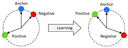
Figure 12: Triplet loss based on cosine similarity (from [69]).

Given a training set, we can see that the number of all possible triplet training samples is cubically larger than the number of training utterances. It is neither efficient nor effective to enumerate all possible triplets [155], and only those that violate the constraint of $s_{n}^{an}-s_{n}^{ap}+\zeta\leq 0$ contributes to the training process. Therefore, how to select informative triplet training samples is fundamental to the effectiveness of the model training. In practice, the “hard negative” sampling strategy is popular [155]. It consists of the following two steps at each epoch:

1. Randomly sample $m$ utterances from each of the $M$ speakers of the training set, which constructs $Mm(m-1)/2$ anchor-positive pairs.

2. For each of the anchor-positive pairs, randomly choose one negative utterance that satisfies $s_{n}^{an}-s_{n}^{ap}+\zeta>0$ from the $(M-1)m$ negative candidates.

Several variants of the “hard negative” sampling were proposed as well. For example, [62] changed the first step by randomly selecting a small number of speakers from the speaker pool instead of from all speakers. In [154], the authors divided training speakers into different groups and constructed each triplet training sample from a single group. Besides the “hard negative” sampling, the “semi-hard” negative sample selection [158, 141] and softmax pre-training [69] are all used to stabilize the training process of the triplet loss.

8.3 Quadruplet loss

Quadruplet loss is a kind of training loss for end-to-end speaker verification where each training sample that contributes to the accumulation of the training objective value independently is constructed from four utterances. Suppose there are a positive pairwise training set $\mathcal{X}_{\rm same}=\{(\mathbf{x}_{n_{1}}^{e},\mathbf{x}_{n_{1}}^{t})|n_{1}=1,2,\cdots,N_{1}\}$ and a negative pairwise training set $\mathcal{X}_{\rm diff}=\{(\mathbf{x}_{n_{2}}^{e},\mathbf{x}_{n_{2}}^{t})|n_{2}=1,2,\cdots,N_{2}\}$ respectively, where $\mathbf{x}_{n_{1}}^{e}$ and $\mathbf{x}_{n_{1}}^{t}$ are from the same speaker while $\mathbf{x}_{n_{2}}^{e}$ and $\mathbf{x}_{n_{2}}^{t}$ are from different speakers. We have $\mathcal{X}_{\rm same}\cup\mathcal{X}_{\rm diff}=\mathcal{X}_{\rm pair}$. Currently, the quadruplet loss is formulated as the maximization of the partial interested area under the ROC curve (pAUC) [86].

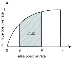
Figure 13: Illustration of the ROC curve, AUC, and pAUC (from [86]).

The maximization of pAUC is to maximize an interested gray area of Fig. 13 that is defined by two hyperparameters $\alpha$ and $\beta$. It has the following three steps:

1. Rank the similarity scores of all pairwise trials in $\mathcal{X}_{\rm diff}$ in descending order, and selecting those elements that rank between the $(\lceil N_{2}\times\alpha\rceil+1)$-th to $\lfloor N_{2}\times\beta\rfloor$-th positions to construct $\mathcal{X}_{\rm diff}^{\prime}=\{(\mathbf{x}_{n_{3}}^{e},\mathbf{x}_{n_{3}}^{t})|n_{3}=1,2,\cdots,N_{3}\}$ where $N_{3}=\lfloor N_{2}\times\beta\rfloor-(\lceil N_{2}\times\alpha\rceil+1)$.

2. Calculate pAUC on $\mathcal{X}_{\rm same}$ and $\mathcal{X}_{\rm diff}^{\prime}$:

   $${\rm pAUC}=1-\frac{1}{N_{1}N_{3}}\sum_{n_{1}=1}^{N_{1}}\sum_{n_{3}=1}^{N_{3}}\Big{(}\delta(s_{n_{1}}<s_{n_{3}})+\frac{1}{2}\delta(s_{n_{1}}=s_{n_{3}})\Big{)}$$ (68)

   where $\delta(\cdot)$ denotes the indicator function, and $s_{n_{1}}$ and $s_{n_{3}}$ denote the cosine similarity of the pairwise trials in $\mathcal{X}_{\rm same}$ and $\mathcal{X}_{\rm diff}^{\prime}$ respectively.

3. Relax the indicator function by the hinge loss which reformulates (68) to:

   $$\mathcal{L}_{\rm pAUC}=\frac{1}{N_{1}N_{3}}\sum_{n_{1}=1}^{N_{1}}\sum_{n_{3}=1}^{N_{3}}{\rm max}\Big{(}0,\zeta-\big{(}s_{n_{1}}-s_{n_{3}})\big{)}\Big{)}^{2}$$ (69)

   where $\zeta$ is a margin hyperparameter.

It can be seen clearly that (69) is a quadruplet loss, since that $(s_{n_{1}}-s_{n_{3}})$ is calculated from four utterances.

[86] proposed two training sample construction methods. The first one is named random sampling. For a mini-batch, it first randomly chooses a mini-batch number of speakers, then randomly selects two utterances for each of the selected speaker, and finally generates the training trials of the batch by pairing all the selected utterances. The second one is named class-center learning. Before training, it first assigns a class center to each speaker in the training set. Then, for each training iteration, it generates the training trials of a mini-batch by pairing each of the class centers with each of the utterances in the batch, where the class centers are updated together with the DNN parameters.

The pAUC based loss has several advantages: (i) it directly optimizes the detection error tradeoff (DET) curve which is the major evaluation metric of speaker verification [156]; (ii) it naturally overcomes the class-imbalanced problem; (iii) it is able to select difficult quadruplet training samples by setting $\alpha=0$ and $\beta$ to a small value, e.g. 0.01; (iv) triplet training samples is a subset of quadruplet training samples when given the same training utterances [156]. Actually the pAUC should be calculated on the entire dataset, however, due to the limited computation resource, (68) is an empirical approximation to it within a mini-batch. Therefore, a large batch size is usually set to reduce the approximation error as much as possible. Fortunately, experimental results demonstrate that a good approximation can be obtained with a batch size of no larger than 512.

8.4 Prototypical network loss

In [25], the prototypical network loss [159], which was originally proposed for few-shot learning, was applied to speaker embedding models. Suppose that a mini-batch contains a support set of $N$ labeled samples $\mathcal{S}=\{(\mathbf{x}_{n},l_{n})|n=1,2,\cdots,N\}$ where $l_{n}\in\{1,2,\cdots,J\}$ is the label of the sample $\mathbf{x}_{n}$, and $\mathcal{S}_{j}$ denotes the set of all samples of class $j$. Then, the prototype of each class is the mean vector of the support points belonging to the class:

$$\mathbf{c}_{j}=\frac{1}{|\mathcal{S}_{j}|}\sum_{(\mathbf{x}_{n},l_{n})\in\mathcal{S}_{j}}\mathbf{x}_{n},\quad j=1,2,\cdots,J$$ (70)

Given a query set $\mathcal{Q}=\{(\mathbf{x}_{q},l_{q})|q=1,2,\cdots,Q\}$ with $l_{q}\in\{1,2,\cdots,J\}$, the prototypical network loss classifies each query point $\mathbf{x}_{q}$ against $J$ prototypes $\{\mathbf{c}_{j}|j=1,2,\cdots,J\}$ via a softmax function:

$$\mathcal{L}_{\rm PNL}=-\sum_{(\mathbf{x}_{q},l_{q})\in Q}{\rm log}\frac{{\rm exp}\Big{(}-d\big{(}\mathbf{x}_{q},\mathbf{c}_{l_{q}}\big{)}\Big{)}}{\sum_{j\prime=1}^{J}{\rm exp}\Big{(}-d\big{(}\mathbf{x}_{q},\mathbf{c}_{j\prime}\big{)}\Big{)}}$$ (71)

where $d(\cdot)$ denotes the squared Euclidean distance.

For each mini-batch, [25] first randomly selects a number of speakers from the training speaker pool, and then randomly chooses a support set and a query set for each of the selected speakers, where the samples of the support set and query set do not overlap. Similar works were also conducted in [160, 161, 162].

Before [25], [78] proposed a generalized end-to-end loss based on the softmax function, which shares a similar idea with the prototypical network loss except that it uses a single set as both the support and query sets. In addition, [163] recently proposed an AM-Centroid loss which replaced the weights of the AAMSoftmax loss function with speaker centroids proposed in [78]. This loss function aims to overcome the weakness of the AAMSoftmax loss based deep networks whose number of parameters at the output layer grows linearly with the number of training speakers.

8.5 Other end-to-end loss functions

Some loss functions cannot be categorized to the above categories. For example, given learnable speaker bases $\{\mathbf{w}_{j}\}_{j}^{J}$ and a mini-batch of utterances $\{(\mathbf{x}_{n},l_{n})\}_{n}^{N}$ where $l_{n}\in\{1,2,\cdots,J\}$, [164] proposed a between-class variation based loss $\mathcal{L}_{\rm BC}$,

$$\mathcal{L}_{\rm BC}=\sum_{j_{2}=1}^{J}\sum_{j_{1}=1,j_{1}\neq j_{2}}^{J}\frac{\mathbf{w}_{j_{1}}^{T}\mathbf{w}_{j_{2}}}{\|\mathbf{w}_{j_{1}}\|\ \|\mathbf{w}_{j_{2}}\|}$$ (72)

and a hard negative mining loss $\mathcal{L}_{\rm H}$,

$$\mathcal{L}_{\rm H}=\sum_{n=1}^{N}\sum_{\mathbf{w}_{h}\in{\rm Hard}_{n}}\!\!{\rm log}\Big{(}1+{\rm exp}\big{(}S(\mathbf{w}_{h},\mathbf{x}_{n})-S(\mathbf{w}_{l_{n}},\mathbf{x}_{n})\big{)}\Big{)}$$ (73)

where $\mathbf{x}_{n}$ denotes the nth utterance, $\mathbf{w}_{l_{n}}$ denotes the basis that $\mathbf{x}_{n}$ belongs to, $S(\cdot)$ is the cosine similarity, and ${\rm Hard}_{n}$ is a set of so-called hard negative speaker bases of $\mathbf{x}_{n}$ which correspond to the top $H$ largest values in $\{S(\mathbf{w}_{j},\mathbf{x}_{n})|{j\neq l_{n}},j=1,2,\cdots,J\}$.

8.6 Discussion to the verification-based loss functions

The verification-based loss functions are fundamentally different from the classification-based loss functions in at least the following aspects. First, speaker verification is essentially an open-set metric learning problem instead of a closed set classification problem. The verification-based losses are consistent with the test pipeline, which directly outputs verification scores.

Second, the output layers of the verification-based losses are very small and irrelevant to the number of training speakers, which is an important advantage of the verification-based methods over classification-based methods. Specifically, the number of parameters of a classification-based network at the output layer grows linearly with the increase of the number of training speakers, which make the network large-scale and easily overfit to the training data. For example, if a training set consists of 50000 speakers and if the top hidden layer of a classification network has 512 hidden units, then the output layer of the network contains 25.6 million parameters. On the contrary, the verification-based systems do not suffer the aforementioned weakness. Aware of this issue, [163] tried to solve the parameter explosion problem by drawing lessons from the prototypical network loss.

The main weakness of the verification-based systems is that they are harder to train than the classification-based systems, since that they need to construct a large number of training trials and then select those that contributes significantly to the effectiveness of the systems, while the classification-based systems just classify each training utterance to its corresponding speaker. To overcome this weakness, many sample selection strategies for selecting highly-informative trials have been developed, such as the hard negative sampling in the triplet loss and the pAUC optimization in the quadruplet loss. Because the highly-informative trials are dynamically changing during the training process, the optimization process is not very stable and consistent. Some unstable examples include the triplet loss or pAUC maximization with the random sampling strategy. Fortunately, this weakness can be alleviated by constructing trials with speaker centroids via, e.g. the class-center learning [86].

In respect of the performance, although the classification-based systems outperformed the verification-based systems once, recently results shown that the latter can achieve competitive performance with the former [86, 162].

A remark: the term “end-to-end” in this section intends to make a difference from the embedding systems in Section 7. However, the term in many other speech processing tasks, which takes raw wave signals as the input and directly output decisions, is broader than the concept here. From the broader concept of “end-to-end”, an end-to-end speaker verification system needs to further integrate additional procedures, including the voice activity detection, cepstral mean and variance normalization, into the network. It also has to prevent using additional back-ends, such as PLDA [105].

9 Speaker diarization

In this section, we overview four kinds of speaker diarization technologies—stage-wise diarization, end-to-end diarization, online diarization, and multimodal diarization, where the stage-wise diarization has been studied for a long time, while the last three are emerging directions.

9.1 Stage-wise speaker diarization

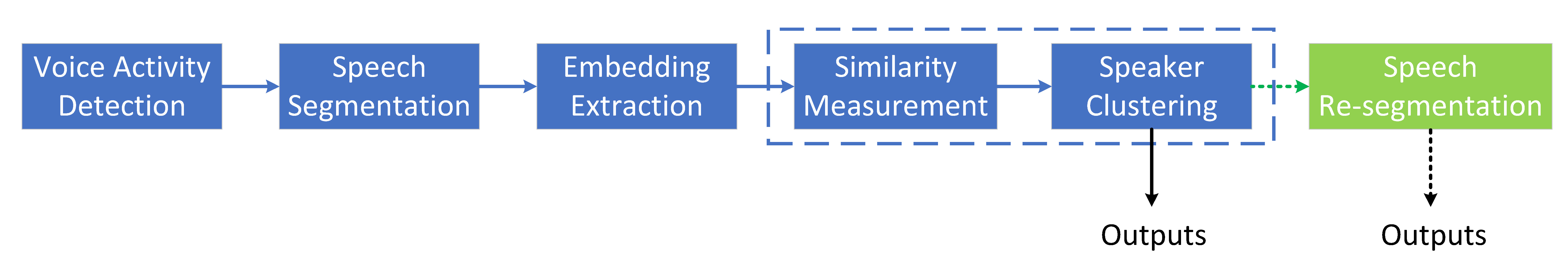
Figure 14: Diagram of the stage-wise speaker diarization, where speech re-segmentation is an optional module.

Stage-wise speaker diarization is composed of multiple independent modules. As shown in Fig. 14, most stage-wise speaker diarization systems consist of four modules—voice activity detection, speech segmentation, speaker feature extraction, and speaker clustering. Some systems also have an optional re-segmentation module. This subsection briefly reviews deep learning based methods for each module. Voice activity detection detects speech in an audio recording and removes non-speech regions. Although it is an important module, it is usually studied independently. Therefore, we focus on reviewing the other modules.

9.1.1 Speech segmentation

Speech segmentation splits speech into multiple speaker-homogeneous segments where each segment belongs to a single speaker. It usually can be categorized to two classes—uniform segmentation and speaker change detection (SCD). Uniform segmentation divides a long audio stream into short segments evenly by a sliding window [165, 166, 167, 168, 169]. For example, a 1.5 seconds sliding window with 0.75 second overlap is a common setting of uniform segmentation.

SCD partitions an audio recording according to the detected speaker change points, which results in non-uniform segments. Generally, it first partitions an audio recording into small segments, then computes the similarity between the two adjacent speech segments in terms of the distance between their representations, and finally decides whether the two adjacent segments are produced from the same speaker by thresholding the distance or finding a local extremum in the consecutive distance stream [155]. A common method for segmenting the audio recording into short segments is to use a sliding window [155, 170]. Recently, an ASR based segmentation [171, 172] is also employed.

Conventional SCD algorithms usually adopt common handcrafted features, e.g. MFCC, as the acoustic representation [173, 174]. An important advantage of the conventional methods is that only the step of tuning the threshold needs some experience, while the other parts do not need training [175]. Recently, the deep speaker embedding features are used as the representation of speech segments instead of conventional handcrafted features [170, 176, 155, 171, 172].

To calculate the similarity between two adjacent segments, Euclidean distance [155] and cosine similarity [170] are two common similarity measurements. Some methods also feed two [172, 176] or more [171] consecutive embeddings together into a pre-trained DNN to predict the similarity between two adjacent segments. Recently, some work formulates SCD as a sequence labeling task, which directly predicts if there is a change point in a speech segment [175, 177, 178].

To summarize, on one side, the uniform segmentation is simple and works fine in many cases, which is the choice of many real-world diarization systems [165, 179, 171]; on the other side, the research on SCD is important not only for speaker diarization but also for many other applications, such as the closed captioning of broadcast television for hearing-impaired people [171].

9.1.2 Speaker feature extraction

The speaker feature extraction module in diarization shares similar technologies with speaker verification. Both of them map speech segments into speaker embeddings by i-vector [179], DNN-UBM/i-vector [180], x-vector [167, 181, 182, 183], or some other deep embedding extractors [184, 169, 185]. See Sections 3 to 8 for the details. Here we only review some embedding methods that utilize additional information for speaker diarization. The authors in [186] incorporated acoustic conditions, such as the distances between speakers and microphones in a meeting or the channel conditions of different speakers in a telephone conversation, into the speaker embeddings, given the fact that the acoustic conditions provide discriminative information for diarization. [187] utilized a graph neural network to refine speaker embeddings, where the local structural information between speech segments is utilized as additional information.

9.1.3 Speaker clustering

Given the segment-level embedding features of an audio recording, speaker clustering aims to partition the speech segments into several groups, each of which belongs to a single speaker. It first defines a similarity measurement for evaluating the similarity of two segments, and then conducts clustering according to the similarity scores. Popular similarity measurements include cosine similarity [169] and PLDA-bases similarity [167, 179]. Recently, some deep-learning-based similarity measurements were also introduced, such as the LSTM-based scoring [188], self-attentive similarity measurement strategies [189], and joint training of speaker embedding and PLDA scoring [166]. Common clustering algorithms include k-means [169], agglomerative hierarchical clustering [167], spectral clustering [188, 169], Bayesian Hidden Markov Model based clustering [181, 182, 183] etc. Recently, Zhang [190] proposed a non-neural-network deep model, named multilayer bootstrap networks, and applied it to speaker clustering [191, 192], which demonstrates competitive performance to the common speaker clustering algorithms. However, these clustering algorithms are unsupervised, which is difficult to utilize manually-labeled training data, e.g. the time-stamped speaker ground truth [193].

To address the problem, some work formulated speaker clustering as a semi-supervised learning problem [194, 195]. Specifically, [194] built a new DNN iteratively from a pre-trained speaker separation DNN for the speaker clustering of each audio file. In [195], the authors proposed an active-learning-based speaker clustering algorithm, which needs some involvement of human labor during the clustering process.

Some work formulated speaker clustering as a supervised learning problem [193, 196, 197]. Specifically, [193] and [196] defined the speaker labels of training data according to their first appearance in the training data. As shown in Fig. 15, given a sequence of speech segments $\mathcal{E}=\{(\mathbf{e}_{n},l_{n})|n=1,2,\cdots,N\}$ where $l_{n}\in\{\rm A,B,C,D,E,\cdots\}$ is the ground truth label of the $n$th segment with each capital letter representing a speaker, the training label of the sequence $\hat{l}_{n}\in\{1,2,3,4,5,\cdots\}$ is tagged with positive integers in the order of the speaker appearance in the sequence. For example, the training labels of the two sequences $[\rm E,A,C,A,E,E,C]$ and $[\rm A,C,A,B,B,C,D,B,D]$ are tagged as $[\rm 1,2,3,2,1,1,3]$ and $[\rm 1,2,1,3,3,2,4,3,4]$ respectively. Under this labeling manner, [193] trained a parameter-sharing RNN clustering model in a supervised way by multiple-instance-learning. They further integrated the RNN with a distance-dependent Chinese restaurant process to address the difficult problem of the unknown number of speakers. An improvement to [193] was further presented in [197]. Additionally, the clustering procedure was also modeled by a discriminative sequence-to-sequence neural network [196].

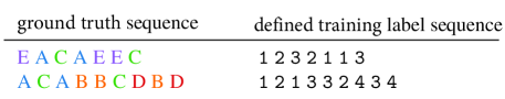
Figure 15: Two examples of the training label sequence definition of the supervised clustering in [196] (from [196]).

9.1.4 Speech re-segmentation

Re-segmentation is an optional step after the speaker clustering. It refines speech boundaries between the speech segments. Variational-Bayesian refinement [198, 167, 199] is the most famous conventional method. Recently, deep learning based re-segmentation methods were also developed. For example, following the successful application of the RNN to voice activity detection and SCD, [200] proposed to address re-segmentation with LSTM.

9.1.5 Speech overlap detection

Most stage-wise speaker diarization systems simply assume that only one person is speaking at any time. In other words, they do not consider the speech overlap problem. However, speech overlap is one of the most important factors that hinder the diarization performance [167, 201, 202, 165], since it happens frequently in practice, e.g. a fast multi-speaker conversation. There have been several traditional studies on overlap detection for speaker diarization [203, 204, 205, 206]. Recently, some deep learning based speech overlap detection methods were also proposed [207, 208]. Specifically, [207] first addressed the overlapped speech detection as a sequence labeling problem by an LSTM-based architecture, and then assigned the detected overlap regions to two speakers by a simple yet effective overlap-aware re-segmentation module. In [208], a region proposal network was first used to detect overlapped speech, and then removed the highly overlapped segments in the post-processing stage. In addition to the above methods, end-to-end speaker diarization, which will be reviewed in the next section, is another way to deal with the speech overlap problem.

9.2 End-to-end speaker diarization

Because conventional clustering algorithms are unsupervised, it cannot minimize the diarization error rate directly [209] and is difficult to deal with the speech overlap problem [209]. Moreover, because each module of the stage-wise speaker diarization in Fig. 14 is optimized independently, the performance is difficult to be boosted. Although several semi-supervised and supervised speaker clustering methods have recently been proposed, the potential of deep neural networks, which are mainly used to extract speaker embeddings in the stage-wise speaker diarization, has not been fully explored yet. To address these problems, [210, 211, 209] proposed an end-to-end diarization method by formulating speaker diarization as a multi-label classification problem.

Figure 16: End-to-end neural diarization with the permutation-free loss for two-speaker diarization (from [209]).

As shown in Fig. 16, given an acoustic feature sequence of an audio recording $\mathcal{Y}=\{\mathbf{y}_{t}\in\mathbb{R}^{d_{1}}|t=1,2,\cdots,T\}$, speaker diarization estimates the speaker label sequence $L=\{\bm{l}_{t}|t=1,2,\cdots,T\}$, where $\bm{l}_{t}=\{l_{t,j}\in\{0,1\}|j=1,2,\cdots,J\}$ denotes a joint activity of a total number of $J$ speakers at time $t$. This multi-label formulation can represent speaker overlap regions properly. For example, $l_{t,j}=l_{t,j^{\prime}}=1$ with $j\neq j^{\prime}$ represents that the speech of the speakers $j$ and $j^{\prime}$ overlaps at time $t$. With the assumption that each speaker is present independently, the frame-wise posteriors are estimated by a neural network as follows [209]:

$$\!\!\mathbf{z}_{t}=[P(l_{t,1}|\mathcal{Y}),P(l_{t,2}|\mathcal{Y}),\cdots,P(l_{t,J}|\mathcal{Y})]={\rm NN}_{t}(\mathcal{Y})\in(0,1)^{J}$$ (74)

where ${\rm NN}_{t}(\cdot)$ denotes a neural network, which was implemented by a BLSTM [211], or a self-attention based neural network [210].

However, a difficult problem for the end-to-end speaker diarization is the speaker-label permutation ambiguity problem when aligning the ground truth label with the speech recording in preparing the training data. For example, given an audio recording with three speakers A, B and C. If the ground-truth label of the recording is “AAABBC” , then the encoded labels “111223” and “222113” are equally correct, making the neural network hard to define a unique training label sequence [212]. To cope with this problem, as shown in Fig. 16, a neural network is trained to minimize the permutation-invariant training (PIT) loss between the output $\mathbf{z}_{t}$ and the reference speaker label $\mathbf{1}_{t}\in\{0,1\}^{J}$ [210, 211, 209]:

$$\mathcal{L}^{PF}=\frac{1}{TJ}\mathop{{\rm min}}_{\phi\in{\rm perm}(J)}\sum_{t}{\rm BCE}(\mathbf{1}_{t}^{\phi},\mathbf{z}_{t})$$ (75)

where ${\rm perm}(J)$ is the set of all possible permutations of the speaker identifiers $\{1,2\cdots,J\}$, and $\mathbf{1}_{t}^{\phi}$ is the $\phi$-th permutation of the ground-truth label sequence, and ${\rm BCE}(\cdot,\cdot)$ is the binary cross entropy between the label and the network output.

Under the multi-label classification framework (74), the end-to-end diarization system is unable to deal with the test scenario where the number of speakers is larger than the maximum number of speakers in any of the training conversations. Here we bravely call this problem the fixed speaker capacity issue for short. To this end, the end-to-end diarization framework is less flexible than the stage-wise methods which can handle any number of speakers in a test conversation [213]. To enlarge the speaker capacity, the number of the output nodes of the neural network (74) tends to be set large. Unfortunately, the computational resource for training with the PIT loss will be exponentially increased along with the increase of the number of the output nodes. To deal with this contradiction, [212] proposed an optimal mapping loss, which directly computes the best match between the output speaker sequence and the ground-truth speaker sequence through a so-called Hungarian algorithm. It reduces the computational complexity to polynomial time, and meanwhile yields similar performance as the PIT loss. It should be noted that, the fixed speaker capacity issue remains unsolved in the optimal mapping loss.

Figure 17: Diagrams of the conventional end-to-end neural diarization (EEND) method with fixed speaker numbers in [209], and the speaker-wise conditional end-to-end neural diarization (SC-EEND) method (from [214]).

To address the fixed speaker capacity issue, [214] proposed a speaker-wise conditional end-to-end (SC-EEND) speaker diarization method. As shown in Fig. 17, it uses an encoder-decoder architecture to decode each speaker’s speech activity iteratively conditioned on the estimated historical speech activities. Although the SC-EEND method achieves increased speaker counting accuracy, it is difficult to handle more than four speakers [214], since it still has to deal with the PIT problem during decoding. Besides, they also proposed an encoder-decoder based attractor calculation method, where a flexible number of speaker attractors are calculated from a speech embedding sequence [213]. However, the speaker capacity of the method remains limited, due to the PIT loss which determines the assignment of the attractors to the training speakers.

9.3 Online speaker diarization

Most state-of-the-art speaker diarization systems work in an offline manner. Online speaker diarization, which outputs the diarization result right after the audio segment arrives, is not an easy task, since that future information is unavailable when analyzing the current segment [215]. In history, a number of online speaker diarization and speaker tracking solutions have been reported [216, 217]. Here we focus on the deep learning based ones, which can be categorized to stage-wise online diarization and end-to-end online diarization methods.

In respect of the stage-wise online diarization, [193] replaced the commonly used clustering module with a trainable unbounded interleaved-state RNN to make prediction in an online fashion, and it was further improved by introducing a sample mean loss [197]. Additionally, a transformer-based discriminative neural clustering model proposed in [196] can also perform online diarization. However, although it is possible to transfer the online clustering to end-to-end speaker diarization, these methods still suffer from the assumption that only one speaker is present in a single segment [215, 212].

In respect of the end-to-end online diarization, [215] extended the self-attention-based end-to-end speaker diarization method in Fig. 16 to an online version, with a speaker-tracing mechanism that is important for the success of the online diarization. Specifically, a straightforward online extension to the framework in Fig. 16 is to perform diarization independently for each chunked recording. However, it is observed that the extension degrades the diarization error rate, due to the speaker permutation inconsistency across the chunk, especially for the short-duration chunks. To overcome this weakness, they applied a speaker-tracing buffer to record the speaker permutation information determined in previous chunks for a correct speaker-tracing in the following chunk. Because this method is limited to two-speaker diarization, more flexible speaker online end-to-end diarization methods need to be further explored [215]. In addition, [218] presented an all-neural approach to simultaneously conduct speaker counting, diarization, and source separation in a block-online manner, where a speaker-tracing mechanism is also employed to avoid the permutation inconsistency problem across time chunks.

9.4 Multimodal speaker diarization

Although speaker diarization is conventionally an audio-only task, the linguistic content carried by speech signals [219] and the speaker behaviors, e.g., the movement of lips, recorded by videos [220] offer valuable supplementary cues to the detection of active speakers. To incorporate the aforementioned knowledge, multimodal speaker diarization is emerging. Here we summarize some work as follows.

The first class is audio-linguistic speaker diarization, [221] integrated lexical cues and acoustic cues together by a gated recurrent unit-based sequence-to-sequence model, which improves the diarization performance by exploring linguistic variability deeply. The effectiveness of using both the linguistic and acoustic cues for diarization has been manifested further in structured scenarios [222, 219] where the speakers are assumed to produce distinguishable linguistic patterns. For instance, a teacher is likely to speak in a more didactic style while a student tends to be more inquisitive; a doctor is likely to inquire on symptoms and prescribe while a patient describe symptoms, etc. Another emerging direction is audio-visual speaker diarization. In [220], the authors proposed a self-supervised audio-video synchronization learning method for the scenario where there lacks massive labeled data. The authors in [223] proposed an iterative audio-visual approach which first enrolls speaker models using audio-visual correspondence, and then combines the enrolled models together with the visual information to determine the active speaker. In addition, microphone arrays provide important spatial information as well. For example, [224] recently combined d-vectors with the spatial information produced from beamforming for the multimodal speaker diarization.

10 Robust speaker recognition

Table 10: Summary of adversarial-training-based domain adaptation methods.

	Variable factors	Instantiation	References
1.	Source and target mappings $M_{s}$ and $M_{t}$	Shared parameters $M_{s}=M_{t}=M$, or unshared parameters $M_{s}\neq M_{t}$.	[225, 226, 227, 228]; [229]
2.	Domain discriminator loss $\mathcal{L}_{{\rm adv}D}$	Binary cross-entropy, multi-class cross-entropy, or Wasserstein distance.	[225]; [230]; [231]
3.	Adversarial loss $\mathcal{L}_{{\rm adv}M}$	The gradient reversal layer, or the GAN loss function.	[225, 226, 232]; [233, 229]
4.	Input feature $\mathbf{X}_{s}$ and $\mathbf{X}_{t}$	Utterance-level speaker features (e.g. i-vector and x-vector), or frame-level acoustic features (e.g. MFCC and F-bank).	[225, 234] ; [226, 232]
5.	Adaptation target	Channel invariant, language invariant, phoneme invariant, noise robust, or short utterance compensation.	[225];[232];[235];[230];[236]

Along with the rapid progress of speaker recognition, the frontier turns to “recognition in the wild” [15, 16, 201], where lots of domain mismatch and noisy problems arise. To overcome these difficulties, many domain adaptation and noise reduction methods were proposed. In this section, we comprehensively review these robust speaker recognition methods, including domain adaptation in Section 10.1, speech enhancement preprocessing in Section 10.2, and data augmentation techniques in Section 10.3.

10.1 Domain adaptation

Over the past few years, speaker recognition has achieved great success due to the application of deep learning and large amount of labeled speech data. However, because collecting and annotating data for every new application is extremely expensive and time-consuming, sufficient training data may not be always available. For example, although large-scale labeled English databases are publicly available, Cantonese databases may be scarce [237]. Hence, it is needed to improve the performance of low-resource speaker recognition by using the large amount of auxiliary data. However, there are many distribution mismatch or domain shift problems between the low-resource data and auxiliary data, including different languages, phonemes, recording equipments, etc., which hinder the effectiveness of the auxiliary data. Fortunately, the mismatch problem can be alleviated by domain adaptation techniques.

Without loss of generality, the domain of interest is called the target domain, and the domain with sufficient labeled training data is called the source domain. The data distributions of the target domain and source domain are denoted as $p_{t}(\mathbf{x},y)$ and $p_{s}(\mathbf{x},y)$ respectively, where $p_{s}(\mathbf{x},y)\neq p_{t}(\mathbf{x},y)$. Domain adaptation uses large amount of labeled data in the source domain to solve the problems in the target domain. If the training data in the target domain is manually labeled, then the domain adaptation is supervised; otherwise, it is unsupervised. This paper focuses on the unsupervised domain adaptation, since it is more common and technically more challenging than the supervised domain adaptation in speaker recognition.

Domain adaptation has long been a significant topic in speaker recognition. It received much attention after the domain adaptation challenge in 2013. Over the past years, lots of supervised [238, 239, 240] and unsupervised [241, 242, 243, 244, 245, 246, 247, 240, 248, 249] shallow domain adaptation methods based on the well known i-vector/PLDA pipline have been developed. Among them, the adaptation is usually accomplished at the back-end, including the methods of compensating the domain mismatch in the i-vector space by an independent module before LDA and PLDA [250, 241, 242, 243], and conducting domain adaptation at LDA [244, 251] or PLDA [238, 245, 239, 246, 247, 240, 248]. Although the methods are quite effective, here we do not discuss their details, as this article focuses on deep learning based ones.

Recently, many deep learning based domain adaptation methods were proposed. Following the categorization of the domain adaptation techniques [252, 253], this paper categorize the deep-learning-based domain adaptation in speaker recognition into the following three classes:

• Adversarial-training-based domain adaptation: It seeks to minimize an approximate domain discrepancy distance through an adversarial objective with a domain discriminator.

• Reconstruction-based domain adaptation: It assumes that the data reconstruction of the source or target samples can be helpful for improving the performance of domain adaptation.

• Discrepancy-based domain adaptation: It aligns the statistical distribution shift between the source and target domains using some mechanisms.

10.1.1 Adversarial-training-based domain adaptation

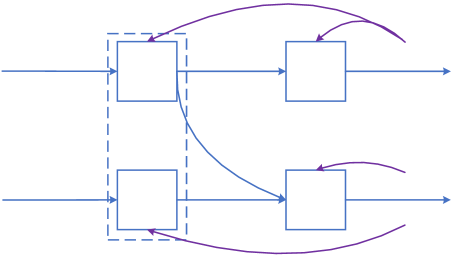
Figure 18: A unified framework of adversarial-training-based domain adaptation.

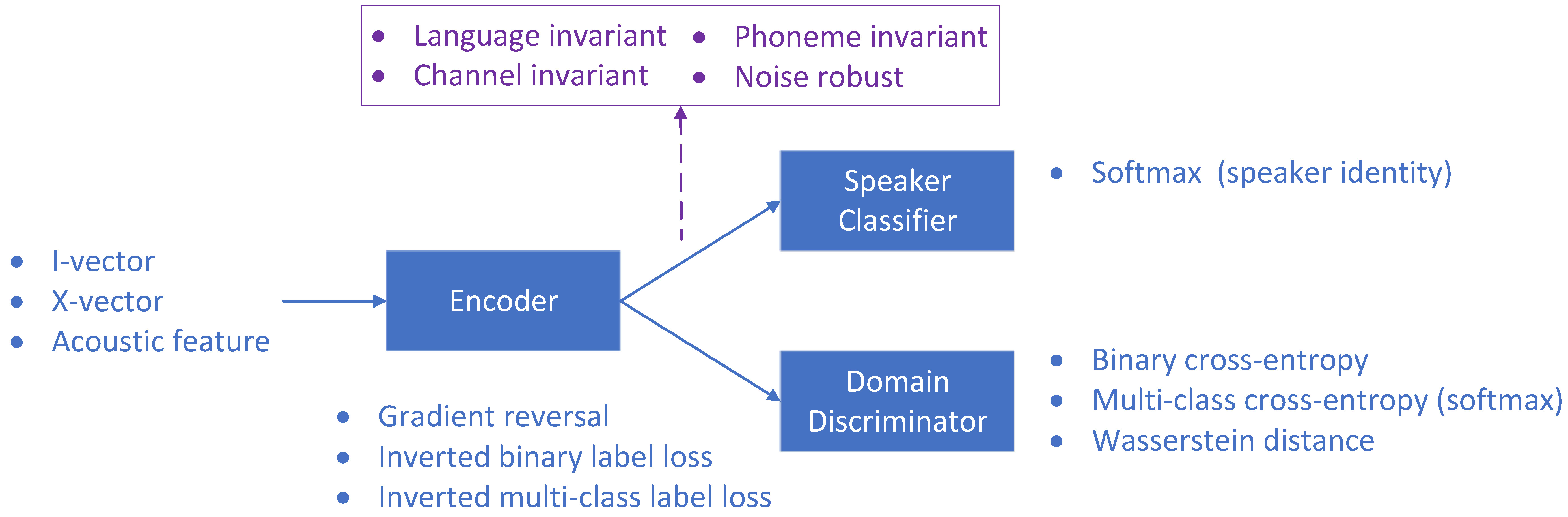
Figure 19: Domain-adversarial neural network (DANN) architecture with $M_{s}=M_{t}=M$.

Before presenting the literature, we first build a unified framework of adversarial-training-based domain adaptation for speaker recognition by drawing lessons from [253]. As shown in Fig. 18, the framework consists of:

• $\mathbf{X}_{s}$ and $Y_{s}$ drawn from $p_{s}(\mathbf{x},y)$ are the source features and speaker labels, and $\mathbf{X}_{t}$ drawn from $p_{t}(\mathbf{x},y)$ are the target features without labels;

• $M_{s}$ and $M_{t}$ are the feature mappings for the source and target domains respectively;

• $C$ is a classifier for discriminating speakers in the source domain.

• $D$ is a domain discriminator for discriminating the source domain and target domain.

The adversarial adaptation methods aim at learning $M_{s}$ and $M_{t}$ for minimizing the distance between the empirical source and target data distributions in the feature space, i.e. making $p(M_{s}(\mathbf{X}_{s}))\approx p(M_{t}(\mathbf{X}_{t}))$. After the adaptation, the recognition models trained on $M_{s}(\mathbf{X}_{s})$ can be directly applied to the target domain.

In the training stage, $M_{s}$ and $C$ are jointly trained using the standard supervised loss:

$$\begin{split}(\hat{M_{s}},\hat{C})&={\rm arg}\mathop{{\rm min}}_{M_{s},C}\mathcal{L}_{\rm cls}(\mathbf{X}_{s},Y_{s};M_{s},C)\\ &=-\mathbb{E}_{(\mathbf{x}_{s},y_{s})\sim(\mathbf{X}_{s},Y_{s})}\sum_{j=1}^{J}\mathbb{I}_{[j=y_{s}]}{\rm log}[C(M_{s}(\mathbf{x}_{s}))]\end{split}$$ (76)

where $J$ is the number of speakers, and $\mathcal{L}_{\rm cls}$ is either the standard softmax or its variants described in Section 7, which ensures that the outputs of $M_{s}$ are speaker-discriminative. To minimize the difference between the source and target representations, the adversarial adaptation methods conduct the following two steps alternatively for $D$ and $M_{t}$:

$$\hat{D}={\rm arg}\mathop{{\rm min}}_{D}\mathcal{L}_{{\rm adv}_{D}}(\mathbf{X}_{s},\mathbf{X}_{t};\hat{M_{s}},\hat{M_{t}},D)$$ (77)

$$\hat{M_{t}}={\rm arg}\mathop{{\rm min}}_{M_{t}}\mathcal{L}_{{\rm adv}_{M}}(\mathbf{X}_{s},\mathbf{X}_{t};\hat{M_{s}},M_{t},\hat{D})$$ (78)

where the symbols with hat, such as $\hat{M_{s}}$, denote that they are fixed during the alternative optimization.

By alternatively minimizing (77) and (78), $D$ and $M_{t}$ play an adversarial game: $D$ is optimized to predict the domain labels of $M_{s}(\mathbf{X}_{s})$ and $M_{t}(\mathbf{X}_{t})$, while $M_{t}$ is trained to make the prediction as incorrect as possible. When the training process converges, we have $p(M_{s}(\mathbf{X}_{s}))\approx p(M_{t}(\mathbf{X}_{t}))$ since that $D$ is unable to discriminate $M_{s}(\mathbf{X}_{s})$ and $M_{t}(\mathbf{X}_{t})$. In addition, because the output of $M_{s}$ is speaker-discriminative which is ensured by the speaker classifier $C$, the output of $M_{t}$ is supposed to be speaker-discriminative too. For clarity, the manual label requirement in (76), (77), and (78) are summarized in Table 11.

Table 11: The manual label requirement in the loss functions (76), (77), and (78). The domain labels can be any factors that are needed to be mitigated, including the types of channels, languages, phonemes, noise, etc.

Losses	Target domain speaker labels	Source domain speaker labels	Domain labels
$\mathcal{L}_{\rm cls}$	✓	✗	✗
$\mathcal{L}_{{\rm adv}_{D}}$	✗	✗	✓
$\mathcal{L}_{{\rm adv}_{M}}$	✗	✗	✓

Different implementations of the framework in Fig. 18 are summarized in Table 10 which will be reviewed in detail as follows.

One of the most popular domain-adversarial neural network (DANN) architectures in literature is shown in Fig. 19 [254]. It consists of an encoder $M$, a speaker classifier $C$, and a domain discriminator $D$. It follows the framework in Fig. 18 with a constraint $M_{s}=M_{t}=M$. Its training alternates the following steps:

1. The encoder is optimized by merging (76) and (78): $\hat{M}={\rm arg}\mathop{{\rm min}}_{M}{\large[}\mathcal{L}_{\rm cls}(\mathbf{X}_{s},Y_{s};M,\hat{C})+\lambda\mathcal{L}_{{\rm adv}_{M}}(\mathbf{X}_{s},\mathbf{X}_{t};M,\hat{D}){\large]}$, where $\lambda$ is a balance factor.

2. The speaker classifier is obtained by minimizing (76): $\hat{C}={\rm arg}\mathop{{\rm min}}_{C}\mathcal{L}_{\rm cls}(\mathbf{X}_{s},Y_{s};\hat{M},C)$.

3. The domain discriminator is obtained by minimizing (77): $\hat{D}={\rm arg}\mathop{{\rm min}}_{D}\mathcal{L}_{{\rm adv}_{D}}(\mathbf{X}_{s},\mathbf{X}_{t};\hat{M},D)$.

After training, the encoder is responsible for extracting domain-invariant and speaker-discriminative speaker features, while the speaker classifier and domain discriminator will be discarded.

The domain-adversarial architecture has been used to explore channel-invariant [225, 226, 227, 228], language-invariant [232, 233, 231, 234, 255], phoneme-invariant [235, 145], noise-robust [230, 256, 257] speaker features, etc. Here we present them briefly as follows.

Figure 20: Channel-invariant domain adaptation (from [226]). The classifier is trained in the same way as the ordinary x-vector. The discriminator is trained on concatenated pairs of within-speaker pairs. The blue arrows represent the forward propagation. The red arrows represent the backward propagation of gradients.

[225] applied DANN to learn a channel invariant feature extractor from the i-vector subspace. It takes the binary cross-entropy loss as the loss function of $\mathcal{L}_{{\rm adv}_{D}}$ to train the discriminator $D$. It adds a gradient reversal layer between the encoder and the discriminator to realize a minimax game $\mathcal{L}_{{\rm adv}_{M}}=-\mathcal{L}_{{\rm adv}_{D}}$. [226] developed a similar framework with Fig. 19 on an x-vector extractor. The framework produces speaker features that are invariant to the granularity of the recording channels. Instead of predicting the concrete domain labels, its domain discriminator predicts whether a pair of speaker embeddings that comes from the same speaker belong to the same recording in a Siamese fashion, see Fig. 20 for the above process. There is also a gradient reversal layer between then x-vector extractor and the domain discriminator. [227] also proposed a similar work to suppress the channel variability.

In addition to the channel mismatch problem, language mismatch is another challenge in speaker recognition. In [232], the authors applied the domain-adversarial architecture directly to acoustic features for a language invariant feature extractor, where the binary cross-entropy loss and a gradient reversal layer are applied to (77) and (78) respectively. In [233], they further replaced the gradient reversal layer with a generative adversarial network (GAN) loss, a.k.a. inverted-label loss. Specifically, $\mathcal{L}_{{\rm adv}_{D}}$ still adopts the binary cross-entropy loss, while $\mathcal{L}_{{\rm adv}_{M}}$ fools the domain discriminator by inverting the domain labels instead of using a gradient reversal layer, i.e.:

$$\begin{split}\mathcal{L}&{}_{{\rm adv}_{D}}(\mathbf{X}_{s},\mathbf{X}_{t};\hat{M},D)=\\ &-\mathbb{E}_{\mathbf{x}_{s}\sim\mathbf{X}_{s}}[{\rm log}(D(\hat{M}(\mathbf{x}_{s})))]-\mathbb{E}_{\mathbf{x}_{t}\sim\mathbf{X}_{t}}[{\rm log}(1-D(\hat{M}(\mathbf{x}_{t})))]\end{split}$$ (79)

$$\begin{split}\mathcal{L}&{}_{{\rm adv}_{M}}(\mathbf{X}_{s},\mathbf{X}_{t};M,\hat{D})=\\ &-\mathbb{E}_{\mathbf{x}_{s}\sim\mathbf{X}_{s}}[{\rm log}(1-\hat{D}(M(\mathbf{x}_{s})))]-\mathbb{E}_{\mathbf{x}_{t}\sim\mathbf{X}_{t}}[{\rm log}(\hat{D}(M(\mathbf{x}_{t})))]\end{split}$$ (80)

where $\mathcal{L}_{{\rm adv}_{D}}$ tags the data from the source domain as “1” and the data from the target domain as “0”, and $\mathcal{L}_{{\rm adv}_{M}}$ takes the opposite domain labels. This objective has the same fixed-point properties as the gradient reversal layer but provides stronger gradients to the encoder than the latter [233, 253].

Figure 21: End-to-end adversarial language adaptation (from [231]).

The authors in [231] trained a language-invariant embedding extractor in an end-to-end fashion, where the embedding extractor is a standard TDNN based x-vector extractor (Fig. 21). They utilized the discriminator to estimate the empirical Wasserstein distance between the source and target samples, and optimized the feature extractor network to minimize the distance in an adversarial manner.

Figure 22: Variational domain adversarial neural network (from [234]).

[234] added an additional variational autoencoder (VAE) branch to the standard DANN structure of Fig. 19 for a language-invariant feature extractor as shown in Fig. 22, where the state-of-the-art x-vector was used as the input. The VAE branch performs like a variational regularization which constrains the learned features to be Gaussian. As we know, Gaussian distribution is essential for the effectiveness of the standard PLDA backend. In [255], they further replaced the VAE with an information-maximized VAE, which not only retains the variational regularization but also inclines to preserve more speaker discriminative information than the VAE.

For text-independent speaker recognition, phonetic information is sometimes harmful, given the fact that it is difficult to ensure shared phonetic coverage across short enrollment and test utterances. However, for long recordings, phonetic information and even more higher level cues, such as word usages, actually differentiates speakers. Quest for such high-level speaker features was an active area of research in about two decades ago. Recently, some studies also investigated its effect on text-independent speaker recognition in the era of deep learning. For example, [145] applied multi-task learning on frame-level layers to enhance the phonetic information in the frame-level features, and used the adversarial training on segment-level layers to learn phoneme-independent representations. Finally, both operations result in improved performance. [235] concluded that phonetic information should be suppressed in text-independent speaker recognition working with frame-wise or extremely short utterances.

Additive noise is one of the most serious interferences of speaker recognition. To explore a noise-robust feature extractor, many works resorted to DANN. For instance, [230] used a multi-class cross entropy loss as the loss function of a noise discriminator to train a noise-condition-invariant feature extractor. [256] applied the adversarial training to learn a feature extractor that are invariant to two kinds of conditions—different environments and different SNRs, where the different environments are represented as a categorical variable and the range of SNRs is formulated as a continuous variable.

[257] applied an unsupervised adversarial invariance (UAI) architecture to disentangle speaker-discriminative information. As shown in Fig. 23, the encoder generates two latent representations $\mathbf{h}_{1}$ and $\mathbf{h}_{2}$ from the x-vector $\mathbf{x}$, where $\mathbf{h}_{1}$ only contains the speaker-discriminative information, and $\mathbf{h}_{2}$ contains all other information of $\mathbf{x}$. This was implemented by optimizing the encoder, predictor and decoder together, where the predictor aims to predict speaker labels $\hat{\mathbf{y}}$ from $\mathbf{h}_{1}$, and the decoder aims to recover $\hat{\mathbf{x}}$ from a concatenation of $\mathbf{h}_{2}$ and a noise corrupted version of $\mathbf{h}_{1}$, denoted as $\mathbf{h}_{1}^{\prime}$. In order to further encourage the “disentanglement”, a minimax game between the disentanglers and the encoder was conducted, where the disentanglers tries to reconstructs the two latent representations from each other, while the encoder is optimized against the disentanglers. An important merit of UAI over DANN is that the adversarial game does not need domain labels.

Figure 23: A brief diagram of unsupervised adversarial invariance.

In addition to DANN where $M_{s}=M_{t}=M$, another kind of adversarial-training-based domain adaptation methods trains an encoder for each domain, i.e. $M_{s}\neq M_{t}$. Adversarial discriminative domain adaptation (ADDA) shown in Fig. 24 is such a representative approach [253]. In [229], the authors applied ADDA to learn an asymmetric mapping that adapts the target domain encoder to the source domain encoder, where the two domains are in different languages.

Figure 24: Adversarial discriminative domain adaptation (ADDA) approach (from [229]). Note that the source encoder is fixed during the adversarial adaptation stage.

From the view of the framework in Fig. 18, ADDA is trained by the following two successive steps:

1. Pre-train a source domain encoder $M_{s}$ and a speaker classifier $C$ with the labeled source data by (76).

2. Fix the source domain encoder $M_{s}$, and perform adversarial training on the target encoder $M_{t}$ and domain discriminator $D$ by alternatively minimizing $\mathcal{L}_{{\rm adv}_{D}}$ and $\mathcal{L}_{{\rm adv}_{M}}$ via (77) and (78) respectively. The domain discriminator $D$ minimizes the binary cross-entropy loss, i.e. $\mathcal{L}_{{\rm adv}_{D}}=-\mathbb{E}_{\mathbf{x}_{s}\sim\mathbf{X}_{s}}[{\rm log}(D(\hat{M}_{s}(\mathbf{x}_{s})))]-\mathbb{E}_{\mathbf{x}_{t}\sim\mathbf{X}_{t}}[{\rm log}(1-D(\hat{M}_{t}(\mathbf{x}_{t})))]$. The target encoder $M_{t}$ minimizes an inverted label loss, i.e. $\mathcal{L}_{{\rm adv}_{M}}=-\mathbb{E}_{\mathbf{x}_{t}\sim\mathbf{X}_{t}}[{\rm log}(\hat{D}(M_{t}(\mathbf{x}_{t})))]$.

In the test stage, the data from the target domain is first mapped to the shared feature space by the target domain encoder, and then classified by a back-end classifier trained in the source domain, e.g. PLDA.

In order to compensate the unreliability of short utterances, [236] proposed to compensate short utterances by long utterances using GAN. Specifically, it uses a generator to generate compensated i-vectors from short-utterance i-vectors, and uses a discriminator to determine whether an i-vector is generated by the generator or extracted from a long utterance. Similarly, [258] addressed the problem by adversely learning a mapping function that maps short embedding features to enhanced embedding features.

Despite of the success of the adversarial-training-based domain adaptation, its training is not easy in practice. For example, DANN learns a common encoder for both domains, which may make the optimization poorly conditioned, since a single encoder has to handle features from two separate domains [253]. Although ADDA is able to learn domain specific encoders, its target domain has no labels. As a result, without shared weights between the encoders, it may quickly fall into a degenerate solution if not properly initialized [253]. To remedy this weakness, a pre-trained source encoder is used to initialize the target encoder, leaving the source encoder fixed during the adversarial training [253, 229]. Besides, many training difficulties observed in related areas, such as image processing, have been encountered in speaker recognition as well, though seldom discussed in depth.

10.1.2 Reconstruction-based domain adaptation

In the machine learning community, CycleGAN, which was originally proposed for image-to-image translation [259], is one of the most common reconstruction-based domain adaptation methods [252]. Recently, it was introduced to speaker recognition [260, 261, 262].

Figure 25: The cycle GAN architecture (from [259]).

As shown in Fig. 25, CycleGAN comprises two generators and two discriminators. The generator $G$ transforms the feature $X$ in a domain to the feature $Y$ in another domain, producing an approximation of $Y$, i.e. $\hat{Y}=G(X)$. The discriminator $D_{Y}$, which aligns with $G$, discriminates between $\hat{Y}$ and $Y$. The other generator-discriminator pair, i.e. $F$ and $D_{X}$, is intended to transfer features from $Y$ to $X$. The generators and discriminators are trained using a cycle consistency loss and a combination of two adversarial losses, where the cycle consistency loss measures how well the original input is reconstructed after a sequence of two generators, i.e. $F(G(X))\approx X$ or $G(F(Y))\approx Y$. Because of the adversarial and cycle reconstruction mechanisms of CycleGAN, it has an outstanding advantage that its training needs neither speaker labels nor paired data between the source and target domains.

At the acoustic feature level, [260] explored a domain adaptation approach by learning feature mappings between a microphone domain and a telephone domain using CycleGAN. It maps the acoustic features from the target domain (microphone) back to the source domain (telephone), and conducts speaker recognition using the system trained in the source domain. In [261], they further investigated the effectiveness of CycleGAN in low resource scenarios where the target domain only has limited amount of data. They found that, the adaptation system trained on limited amount of target domain data performs slightly better than the adaptation system trained on a larger amount of target domain data, when some noise was added to the data. In [262], they developed a CycleGAN-based feature enhancement approach in the log-filter bank space to improve the performance of speaker verification in noisy and reverberant environments.

Besides CycleGAN, the encoder-decoder structure is another popular reconstruction-based domain adaptation method in machine learning [252]. As for speaker recognition, [263] combined an autoencoder with a denoising autoencoder to adapt resource-rich source domain data to the target domain.

10.1.3 Discrepancy-based domain adaptation

Discrepancy-based domain adaptation aligns the statistical distribution shift between the source and target domains by using some statistic criteria, including maximum mean discrepancy (MMD), correlation alignment (CORAL), Kullback-Leibler divergence, etc. For speaker verification, those criteria has been widely studied in shallow domain adaptation models [243, 246]. Recently, some of them were also introduced to the deep learning based adaptation approaches. Specifically, [264] added a MMD based loss to the reconstruction loss of an autoencoder to train a domain-invariant encoder for multi-source adaptation of i-vectors. In [265, 266], they further proposed a nuisance-attribute autoencoder based on MMD. In [267], they proposed a multi-level deep neural network adaptation method using MMD and consistency regularization.

10.2 Speech enhancement and de-reverberation preprocessing

Speech is always distorted by noise and reverberation in real-world scenarios. A natural choice of coping with these distortions for speaker recognition is to add a speech enhancement or de-reverberation preprocessing module. Recently, deep learning based speech enhancement and de-reverberation techniques [268] have been applied to speaker recognition, which can be roughly divided into three categories, i.e. masking-based [269, 270, 271, 272, 273], mapping-based [274, 275, 276, 277, 278], and GAN-based [279] techniques. It should be note that this section only reviews some general concepts and provides useful cues without considering the details of the speech enhancement techniques, since it is out the scope of this paper. More details can be found in speech enhancement related papers [268].

Masking-based speech enhancement has received a lot of attention and shown impressive performance in speech quality and speech intelligibility. It uses a DNN to estimate a time-frequency mask of noisy speech, and then uses the mask to recover the corresponding clean speech. In [269, 270, 271], the authors applied masking-based speech enhancement techniques as an independently noise reduction module for speaker recognition. In [272], the authors jointly optimized speech separation and speaker verification networks together. Besides, [273] designed a VoiceID loss which jointly optimize a pre-trained speaker embedding system and a speech enhancement network where the speaker embedding system is fixed during the joint optimization, as shown in Fig. 26.

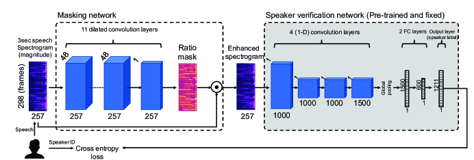
Figure 26: Flow chart of the VoiceID loss (from [273]).

DNN-based autoencoder, which maps noisy speech directly to its clean counterpart, is another speech enhancement method for speaker recognition. [274] trained an autoencoder to map the log magnitude spectrum of noisy speech to its clean counterpart by minimizing the mean squared error, which demonstrated its effectiveness on the text-dependent GMM-MAP and text-independent i-vector systems. The authors of [275] explored a similar noise reduction method with [274], and applied it to an x-vector system [276]. In [277], the authors enhanced both the amplitude feature and the phase feature, where they used MFCC as the amplitude feature, and modified group delay cepstral coefficients as the phase feature. They concluded that simultaneous enhancing the amplitude and phase features is more effective than enhancing their individual components alone. Apart from the simplest feedforward DNN, more complicated LSTM based speech enhancement methods were also explored [278].

Besides the masking and mapping based speech enhancement, GAN-based speech enhancement methods for speaker recognition were also developed. In specific, [279] used conditional GANs to learn a mapping from a noisy spectrum to its enhanced counterpart. The conditional GAN consists of a generator and a discriminator which are trained in an adversarial manner. The generator enhances the noisy spectrum; the discriminator aims to distinguish the enhanced spectrum from their clean counterpart using the noisy spectrum as a condition. In addition, [280] proposed a noise robust bottleneck feature extraction method based on adversarial training.

In addition to the above speech enhancement methods for speaker recognition, speech de-reverberation has also been studied in speaker recognition [281, 282, 283]. Recently, far-field and multi-channel speaker recognition also attracted much attention [284, 285, 286, 287].

10.3 Data augmentation for robust speaker recognition

Large-scale multi-condition training is an effective way to improve the generalization of speaker recognition in noisy environments. Particularly, we have observed that the performance of deep speaker embedding systems appear to be highly dependent on the amount of training data. One way to prepare large-scale noisy training data is data augmentation. In [14], the authors employed additive noises and reverberation to the original training data for the data augmentation of x-vectors, which has shown to be very effective. [288] applied a mixup learning strategy to improve the generalization of x-vector extractors. To improve the performance of speaker verification for children with limited data, [289] made speed and pitch perturbation as well as voice conversion to increase the amount of training data. Besides, [290] validated the effectiveness of spectral augmentation, which was originally proposed for speech recognition, for deep speaker embeddings.

10.4 Other robust methods

Apart from the aforementioned methods, some other robust speaker recognition methods are as follows. For example, [291] optimized a deep feature loss for feature-domain enhancement of x-vector extractors. [292] designed a new loss function for noise-robust speaker recognition. [70] proposed an orthogonal vector pooling strategy to remove unwanted factors. There are also many robust back-ends for speaker verification [293, 294, 295, 296, 297].

11 Datasets

Table 12: Popular databases and challenges for speaker recognition. The term “wild” denotes that the audio is acquired across unconstrained conditions. The term “quite” denotes that the data were recorded indoor under a typical office environment. The term “SV”,“SI” and “SR” are the abbreviations of “speaker verification”, “speaker identification” and “speaker recognition” respectively.

Dataset	Year	Condition	Language	Sample rate	Application	Speakers	Data amount	Annotation method
NIST SRE [298]	1996 $\sim$ 2020	Clean, noisy	Multilingual	—	Text-independent SR	—	—	Hand annotated
VoxCeleb1 [15]	2017	Multi-media (wild)	Mostly English	16kHZ	Text-independent SV and SI	1,251 (690 males)	153,516 utterances, 352 hours	Automated pipeline
VoxCeleb2 [59]	2018	Multi-media (wild)	Multilingual Mostly English	—	Text-independent SV and SI	6,112 (3761 males)	1,128,246 utterances, 2,442 hours	Automated pipeline
SITW [16]	2016	Multi-media (wild)	—	16kHZ	Text-independent single and multi-speaker SV	299 (203 males)	2,800 utterances	Hand annotated
RSR2015 [299]	2015	Smart-phones and tablets (quite)	English	16 kHZ	Text-dependent SV	300 (157 males)	196,844 files, 151 hours	Hand annotated
RedDots [300]	2015	Mobile devices (through internet)	English	—	Fixed phrase, free speech and text-prompted SV	45	—	Manual, automatic, or semi-automatic
VOICES [301, 302]	2018	Far-field microphones (noisy room)	English	48 kHZ	Text-independent SV and SI	300	374,688 files, 1440 hours	Hand annotated
Librispeech[303]	2015	—	English	16 kHz	ASR and SR	Over 9,000	1000 hours	Manually annotated
CN-CELEB[304]	2019	Multi-media (wild)	Chinese	—	Text-independent SV	1000	130,109 utterances, 274 hours	Automated pipeline with human check
BookTubeSpeech [305]	2020	Multi-media	—	—	Text-independent SV	8450	—	Automatic pipeline
Hi-MIA [306]	2020	Microphone arrays (rooms, far-field)	Chinese, English	16kHZ, 44.1kHz	Text-dependent SV	340 (175 male)	More than 3,936,003 utterance, 1,561 hours	Hand annotated
FFSVC 2020 [307]	2020	Close-talk cellphone, far-field microphone arrays (far-field)	Mandarin	16kHZ, 48kHZ	Text-dependent and text-independent SV	—	—	Hand annotated
DIHARD1 [201]	2018	Single channel (wild)	English (most), Mandarin	16kHZ	Speaker diarization	—	40 hours	Hand annotated
DIHARD2 [308]	2019	Single channel and multichannel (wild)	English (most), Mandarin	16kHZ	Speaker diarization	—	503 files, 339.95 hours	Hand annotated
AMI [309]	2005	Multi-modal	English	—	Speaker diarization	—	100 hours	Hand annotated

In this section, we make an overview to existing challenges, and datasets for speaker recognition.

Table 12 summarizes the brief information of most common and some recently developed datasets. The recording methods of the databases are briefly introduced as follows.

• NIST SRE: The National Institute of Standards and Technology (NIST) of America has successfully conducted 15 Speaker Recognition Evaluations (SREs) in the past 20 years. It is the largest and most popular challenge in speaker recognition. More information can be found in [298, 310].

• VoxCeleb1,2: The VoxCeleb dataset was collected by a fully automated pipeline based on computer vision techniques from open-source media. The pipeline obtains videos from YouTube, performs active speaker verification using a two-stream synchronization CNN, and confirms the identity of the speaker using CNN based facial recognition [15, 59].

• SITW: The speakers in the wild (SITW) database contains hand-annotated speech samples from open-source media for the purpose of benchmarking text-independent speaker recognition technology on single and multi-speaker audio acquired across unconstrained conditions [16].

• RSR2015: The RSR2015 database were recorded indoor under a typical office environment with six mobile devices (five smart-phones and one tablet) [299].

• RedDots: The RedDots project used a mobile app as the recording front-end. Speakers recorded their voices offline and later on uploaded the recordings to an Apache web server when Internet connection was available [300].

• VOICES: The voices obscured in complex environmental settings (VOICES) corpus was recorded in furnished rooms with background noise played in conjunction with foreground speech selected from the LibriSpeech corpus. The displayed noises includes television, music, or overlapping speech from multiple speakers (referred to as babble) [301, 302].

• LibriSpeech: While intended created for speech recognition rather than verification or diarization, LibriSpeech does include labels of speaker identities and is thus useful for speaker recognition [303, 305].

• CN-CELEB: CN-CELEB was collected following a two-stage strategy: firstly the authors used an automated pipeline to extract potential segments of the Person of Interest from “bilibili.com”, and then they applied a human check to remove incorrect segments [304].

• BookTubeSpeech: The BookTubeSpeech was collected by an automatic pipeline from BookTube videos [305].

• Hi-MIA: Hi-MIA database was designed for far-field scenarios. Recordings were captured by multiple microphone arrays located in different directions and distance to the speaker and a high-fidelity close-talking microphone [306].

• FFSVC 2020: The far-field speaker verification challenge 2020 (FFSVC20) is designed to boost the speaker verification research with special focus on far-field distributed microphone arrays under noisy conditions in real scenarios [311, 307].

• DIHARD1,2: The DIHARD challenge intended to improve the robustness of diarization systems to variation in recording equipment, noise conditions, and conversational domain [201, 308].

• AMI: The AMI meeting corpus is a multi-modal data set consisting of 100 hours of meeting recordings, and it was recorded using a wide range of devices including close-talking and far-field microphones, individual and room-view video cameras, projection, a whiteboard, and individual pens, all of which produce output signals that are synchronized with each other [309].

12 Conclusions and discussions

This paper has provided a comprehensive overview of the deep learning based speaker recognition. We have analysed the relationship between different subtasks, including speaker verification, identification, and diarization, and summarized some common difficulties. Based on the analysis, we summarized the subtasks from three widely studied core issues—speaker feature extraction, speaker diarization, and robust speaker recognition. For speaker feature extraction, we reviewed two kinds of hybrid structures, which are DNN-UBM/i-vector and DNN-BNF/i-vector. In addition, the overview of the state-of-the-art deep speaker embedding were made in respect of four key components, which are the inputs, network structures, temporal pooling strategies, and loss functions respectively. Particularly, we reviewed the loss functions of the end-to-end speaker verification for feature learning from the perspective of different training sample construction methods. For speaker diarization, we reviewed stage-wise diarization, supervised end-to-end diarization, online diarization, and multimodal diarization. For robust speaker recognition, we surveyed three kinds of deep learning based domain adaptation methods as well as several speech preprocessing methods, which deal with the domain mismatch and back-ground noise respectively. Some popular and recently developed datasets were summarized as well. To conclude, deep learning has boosted the performance of speaker recognition to a new high level. We make our best to summarize the recent rapid progress of the deep learning based speaker recognition, hopefully this provides a knowledge resource and further blooms the research community.

Although the deep learning based speaker recognition has achieved a great success, many issues remain to be addressed. Here we list some open problems from the perspectives of network training, loss functions, real-world diarization, and domain adaptation respectively. For the network training, most speaker feature extraction methods need handcraft acoustic features as the input, which may not be optimal. The state-of-the-art deep models have a large number of parameters, which are difficult to be applied to portable devices. The network training also needs large amounts of labeled training data and heavy computation resources. For the loss functions, although so many loss functions have been proposed, there is lack of strong theoretical base for the success of the loss functions, nor theoretical guidance that could lead to better loss functions. Although the verification losses for the end-to-end speaker verification meet the verification process tightly, their potentials have not been fully developed yet. For the real-world diarization, from the recent DIHARD challenges, one can see that speaker diarization is still a hard problem. In a real-world conversation, a speech recording may be contaminated by serious speech overlap and strong background noise. Some technically difficult problems, such as the unknown number of speakers and rapid speaker changes, also hinder the performance of speaker diarization in real-world applications severely. Finally, although many domain adaptation algorithms have been proposed, especially those based on adversarial learning, they have not made landmark progress compared to traditional shallow adaptation methods, e.g. the PLDA based adaptation, which needs further efforts.

13 Acknowledgement

The authors are grateful to Prof. DeLiang Wang, the Co-Editor-in-Chief, and the anonymous reviewers for their valuable comments, which helped greatly improve the quality of the paper. The authors would also like to thank our colleagues Meng-Zhen Li and Rui Wang for their helpful discussions.

References

- [1] T. Kinnunen, H. Li, An overview of text-independent speaker recognition: From features to supervectors, Speech communication 52 (1) (2010) 12–40.
- [2] J. P. Campbell, W. Shen, W. M. Campbell, R. Schwartz, J.-F. Bonastre, D. Matrouf, Forensic speaker recognition, IEEE Signal Processing Magazine 26 (2) (2009) 95–103.
- [3] C. Champod, D. Meuwly, The inference of identity in forensic speaker recognition, Speech communication 31 (2-3) (2000) 193–203.
- [4] R. Togneri, D. Pullella, An overview of speaker identification: Accuracy and robustness issues, IEEE circuits and systems magazine 11 (2) (2011) 23–61.
- [5] S. Pruzansky, M. V. Mathews, Talker-recognition procedure based on analysis of variance, The Journal of the Acoustical Society of America 36 (11) (1964) 2041–2047.
- [6] D. A. Reynolds, T. F. Quatieri, R. B. Dunn, Speaker verification using adapted gaussian mixture models, Digital signal processing 10 (1-3) (2000) 19–41.
- [7] W. M. Campbell, D. E. Sturim, D. A. Reynolds, Support vector machines using GMM supervectors for speaker verification, IEEE signal processing letters 13 (5) (2006) 308–311.
- [8] P. Kenny, G. Boulianne, P. Ouellet, P. Dumouchel, Joint factor analysis versus eigenchannels in speaker recognition, IEEE Transactions on Audio, Speech, and Language Processing 15 (4) (2007) 1435–1447.
- [9] N. Dehak, P. J. Kenny, R. Dehak, P. Dumouchel, P. Ouellet, Front-end factor analysis for speaker verification, IEEE Transactions on Audio, Speech, and Language Processing 19 (4) (2010) 788–798.
- [10] P. Kenny, Bayesian speaker verification with heavy-tailed priors., in: Odyssey, Vol. 14, 2010.
- [11] D. Garcia-Romero, C. Y. Espy-Wilson, Analysis of i-vector length normalization in speaker recognition systems, in: Twelfth annual conference of the international speech communication association, 2011.
- [12] Y. Lei, N. Scheffer, L. Ferrer, M. McLaren, A novel scheme for speaker recognition using a phonetically-aware deep neural network, in: 2014 IEEE International Conference on Acoustics, Speech and Signal Processing (ICASSP), IEEE, 2014, pp. 1695–1699.
- [13] E. Variani, X. Lei, E. McDermott, I. L. Moreno, J. Gonzalez-Dominguez, Deep neural networks for small footprint text-dependent speaker verification, in: 2014 IEEE International Conference on Acoustics, Speech and Signal Processing (ICASSP), IEEE, 2014, pp. 4052–4056.
- [14] D. Snyder, D. Garcia-Romero, G. Sell, D. Povey, S. Khudanpur, X-vectors: Robust DNN embeddings for speaker recognition, in: 2018 IEEE International Conference on Acoustics, Speech and Signal Processing (ICASSP), IEEE, 2018, pp. 5329–5333.
- [15] A. Nagrani, J. S. Chung, A. Zisserman, VoxCeleb: A large-scale speaker identification dataset, Proc. Interspeech 2017 (2017) 2616–2620.
- [16] M. McLaren, L. Ferrer, D. Castan, A. Lawson, The speakers in the wild (SITW) speaker recognition database., in: Interspeech, 2016, pp. 818–822.
- [17] J. H. Hansen, T. Hasan, Speaker recognition by machines and humans: A tutorial review, IEEE Signal processing magazine 32 (6) (2015) 74–99.
- [18] D. A. Reynolds, An overview of automatic speaker recognition technology, in: 2002 IEEE International Conference on Acoustics, Speech, and Signal Processing, Vol. 4, IEEE, 2002, pp. IV–4072.
- [19] A. Fazel, S. Chakrabartty, An overview of statistical pattern recognition techniques for speaker verification, IEEE Circuits and Systems Magazine 11 (2) (2011) 62–81.
- [20] Z. Wu, N. Evans, T. Kinnunen, J. Yamagishi, F. Alegre, H. Li, Spoofing and countermeasures for speaker verification: A survey, speech communication 66 (2015) 130–153.
- [21] X. Anguera, S. Bozonnet, N. Evans, C. Fredouille, G. Friedland, O. Vinyals, Speaker diarization: A review of recent research, IEEE Transactions on Audio, Speech, and Language Processing 20 (2) (2012) 356–370.
- [22] R. K. Das, X. Tian, T. Kinnunen, H. Li, The attacker’s perspective on automatic speaker verification: An overview, arXiv preprint arXiv:2004.08849.
- [23] A. Irum, A. Salman, Speaker verification using deep neural networks: A review, International Journal of Machine Learning and Computing 9 (1) (2019) 20–25.
- [24] S. Yadav, A. Rai, Learning discriminative features for speaker identification and verification., in: Interspeech, 2018, pp. 2237–2241.
- [25] J. Wang, K.-C. Wang, M. T. Law, F. Rudzicz, M. Brudno, Centroid-based deep metric learning for speaker recognition, in: ICASSP 2019-2019 IEEE International Conference on Acoustics, Speech and Signal Processing (ICASSP), IEEE, 2019, pp. 3652–3656.
- [26] R. Ji, X. Cai, X. Bo, An end-to-end text-independent speaker identification system on short utterances, Proc. Interspeech 2018 (2018) 3628–3632.
- [27] Q. Hong, C. Wu, H. Wang, C. Huang, Combining deep embeddings of acoustic and articulatory features for speaker identification, in: ICASSP 2020 - 2020 IEEE International Conference on Acoustics, Speech and Signal Processing (ICASSP), 2020, pp. 7589–7593.
- [28] N. Flemotomos, D. Dimitriadis, A memory augmented architecture for continuous speaker identification in meetings, in: ICASSP 2020 - 2020 IEEE International Conference on Acoustics, Speech and Signal Processing (ICASSP), 2020, pp. 6524–6528.
- [29] D. Snyder, X-vectors: Robust neural embeddings for speaker recognition, Ph.D. thesis, Johns Hopkins University (2020).
- [30] P. Kenny, P. Ouellet, N. Dehak, V. Gupta, P. Dumouchel, A study of interspeaker variability in speaker verification, IEEE Transactions on Audio, Speech, and Language Processing 16 (5) (2008) 980–988.
- [31] S. Dey, S. Madikeri, M. Ferras, P. Motlicek, Deep neural network based posteriors for text-dependent speaker verification, in: 2016 IEEE International Conference on Acoustics, Speech and Signal Processing (ICASSP), IEEE, 2016, pp. 5050–5054.
- [32] H. Zeinali, L. Burget, H. Sameti, O. Glembek, O. Plchot, Deep neural networks and hidden markov models in i-vector-based text-dependent speaker verification., in: Odyssey, 2016, pp. 24–30.
- [33] Y. Lei, L. Ferrer, M. McLaren, N. Scheffer, A deep neural network speaker verification system targeting microphone speech, in: Fifteenth Annual Conference of the International Speech Communication Association, 2014.
- [34] S. Dey, P. Motlicek, S. Madikeri, M. Ferras, Exploiting sequence information for text-dependent speaker verification, in: 2017 IEEE International Conference on Acoustics, Speech and Signal Processing (ICASSP), Ieee, 2017, pp. 5370–5374.
- [35] H. Zeinali, H. Sameti, L. Burget, et al., Text-dependent speaker verification based on i-vectors, neural networks and hidden markov models, Computer Speech & Language 46 (2017) 53–71.
- [36] F. Richardson, D. Reynolds, N. Dehak, Deep neural network approaches to speaker and language recognition, IEEE signal processing letters 22 (10) (2015) 1671–1675.
- [37] P. Kenny, T. Stafylakis, P. Ouellet, V. Gupta, M. J. Alam, Deep neural networks for extracting Baum-Welch statistics for speaker recognition., in: Odyssey, Vol. 2014, 2014, pp. 293–298.
- [38] D. Snyder, D. Garcia-Romero, D. Povey, Time delay deep neural network-based universal background models for speaker recognition, in: 2015 IEEE Workshop on Automatic Speech Recognition and Understanding (ASRU), IEEE, 2015, pp. 92–97.
- [39] M. McLaren, Y. Lei, L. Ferrer, Advances in deep neural network approaches to speaker recognition, in: 2015 IEEE international conference on acoustics, speech and signal processing (ICASSP), IEEE, 2015, pp. 4814–4818.
- [40] L. Chen, K. A. Lee, B. Ma, W. Guo, H. Li, L.-R. Dai, Phone-centric local variability vector for text-constrained speaker verification, in: Sixteenth Annual Conference of the International Speech Communication Association, 2015.
- [41] F. Richardson, D. A. Reynolds, N. Dehak, A unified deep neural network for speaker and language recognition, in: Sixteenth Annual Conference of the International Speech Communication Association, 2015.
- [42] S. O. Sadjadi, S. Ganapathy, J. W. Pelecanos, The IBM 2016 speaker recognition system, arXiv preprint arXiv:1602.07291.
- [43] M. McLaren, Y. Lei, N. Scheffer, L. Ferrer, Application of convolutional neural networks to speaker recognition in noisy conditions, in: Fifteenth Annual Conference of the International Speech Communication Association, 2014.
- [44] D. Garcia-Romero, A. McCree, Insights into deep neural networks for speaker recognition, in: Sixteenth Annual Conference of the International Speech Communication Association, 2015.
- [45] H. Zheng, S. Zhang, W. Liu, Exploring robustness of DNN/RNN for extracting speaker Baum-Welch statistics in mismatched conditions, in: Sixteenth Annual Conference of the International Speech Communication Association, 2015.
- [46] S. H. Ghalehjegh, R. C. Rose, Deep bottleneck features for i-vector based text-independent speaker verification, in: 2015 IEEE Workshop on Automatic Speech Recognition and Understanding (ASRU), IEEE, 2015, pp. 555–560.
- [47] M. McLaren, L. Ferrer, A. Lawson, Exploring the role of phonetic bottleneck features for speaker and language recognition, in: 2016 IEEE International Conference on Acoustics, Speech and Signal Processing (ICASSP), IEEE, 2016, pp. 5575–5579.
- [48] A. Lozano-Diez, A. Silnova, P. Matejka, O. Glembek, O. Plchot, J. Pesan, L. Burget, J. Gonzalez-Rodriguez, Analysis and optimization of bottleneck features for speaker recognition., in: Odyssey, 2016, pp. 352–357.
- [49] C.-T. Do, C. Barras, V.-B. Le, A. Sarkar, Augmenting short-term cepstral features with long-term discriminative features for speaker verification of telephone data, in: INTERSPEECH, 2013, pp. 3562–3566.
- [50] A. K. Sarkar, C.-T. Do, V.-B. Le, C. Barras, Combination of cepstral and phonetically discriminative features for speaker verification, IEEE Signal Processing Letters 21 (9) (2014) 1040–1044.
- [51] D. Snyder, D. Garcia-Romero, D. Povey, S. Khudanpur, Deep neural network embeddings for text-independent speaker verification., in: Interspeech, 2017, pp. 999–1003.
- [52] H. Muckenhirn, M. M. Doss, S. Marcell, Towards directly modeling raw speech signal for speaker verification using CNNs, in: 2018 IEEE International Conference on Acoustics, Speech and Signal Processing (ICASSP), IEEE, 2018, pp. 4884–4888.
- [53] M. Ravanelli, Y. Bengio, Speaker recognition from raw waveform with sincnet, in: 2018 IEEE Spoken Language Technology Workshop (SLT), IEEE, 2018, pp. 1021–1028.
- [54] J.-w. Jung, H.-s. Heo, I.-h. Yang, H.-j. Shim, H.-j. Yu, Avoiding speaker overfitting in end-to-end DNNs using raw waveform for text-independent speaker verification, Proc. Interspeech 2018 (2018) 3583–3587.
- [55] J.-W. Jung, H.-S. Heo, I.-H. Yang, H.-J. Shim, H.-J. Yu, A complete end-to-end speaker verification system using deep neural networks: From raw signals to verification result, in: 2018 IEEE International Conference on Acoustics, Speech and Signal Processing (ICASSP), IEEE, 2018, pp. 5349–5353.
- [56] J.-w. Jung, H.-S. Heo, J.-h. Kim, H.-j. Shim, H.-J. Yu, RawNet: Advanced end-to-end deep neural network using raw waveforms for text-independent speaker verification, Proc. Interspeech 2019 (2019) 1268–1272.
- [57] J.-w. Jung, H.-S. Heo, H.-j. Shim, H.-J. Yu, Short utterance compensation in speaker verification via cosine-based teacher-student learning of speaker embeddings, in: 2019 IEEE Automatic Speech Recognition and Understanding Workshop (ASRU), IEEE, 2019, pp. 335–341.
- [58] Y.-Q. Yu, L. Fan, W.-J. Li, Ensemble additive margin softmax for speaker verification, in: ICASSP 2019-2019 IEEE International Conference on Acoustics, Speech and Signal Processing (ICASSP), IEEE, 2019, pp. 6046–6050.
- [59] J. S. Chung, A. Nagrani, A. Zisserman, VoxCeleb2: Deep speaker recognition, Proc. Interspeech 2018 (2018) 1086–1090.
- [60] W. Xie, A. Nagrani, J. S. Chung, A. Zisserman, Utterance-level aggregation for speaker recognition in the wild, in: ICASSP 2019-2019 IEEE International Conference on Acoustics, Speech and Signal Processing (ICASSP), IEEE, 2019, pp. 5791–5795.
- [61] S. Yadav, A. Rai, Frequency and temporal convolutional attention for text-independent speaker recognition, in: ICASSP 2020 - 2020 IEEE International Conference on Acoustics, Speech and Signal Processing (ICASSP), 2020, pp. 6794–6798.
- [62] C. Zhang, K. Koishida, End-to-end text-independent speaker verification with triplet loss on short utterances., in: Interspeech, 2017, pp. 1487–1491.
- [63] C. Zhang, K. Koishida, J. H. Hansen, Text-independent speaker verification based on triplet convolutional neural network embeddings, IEEE/ACM Transactions on Audio, Speech, and Language Processing 26 (9) (2018) 1633–1644.
- [64] Y. Zhang, M. Yu, N. Li, C. Yu, J. Cui, D. Yu, Seq2seq attentional siamese neural networks for text-dependent speaker verification, in: ICASSP 2019-2019 IEEE International Conference on Acoustics, Speech and Signal Processing (ICASSP), IEEE, 2019, pp. 6131–6135.
- [65] Y. Zhu, B. Mak, Orthogonal training for text-independent speaker verification, in: ICASSP 2020 - 2020 IEEE International Conference on Acoustics, Speech and Signal Processing (ICASSP), 2020, pp. 6584–6588.
- [66] Y. Zhu, B. Mak, Orthogonality regularizations for end-to-end speaker verification, in: Proc. Odyssey 2020 The Speaker and Language Recognition Workshop, 2020, pp. 17–23.
- [67] D. Garcia-Romero, A. McCree, D. Snyder, G. Sell, JHU-HLTCOE System for the Voxsrc Speaker Recognition Challenge, in: ICASSP 2020 - 2020 IEEE International Conference on Acoustics, Speech and Signal Processing (ICASSP), 2020, pp. 7559–7563.
- [68] Z. Wang, K. Yao, X. Li, S. Fang, Multi-resolution multi-head attention in deep speaker embedding, in: ICASSP 2020 - 2020 IEEE International Conference on Acoustics, Speech and Signal Processing (ICASSP), 2020, pp. 6464–6468.
- [69] C. Li, X. Ma, B. Jiang, X. Li, X. Zhang, X. Liu, Y. Cao, A. Kannan, Z. Zhu, Deep speaker: an end-to-end neural speaker embedding system, arXiv preprint arXiv:1705.02304.
- [70] I. Kim, K. Kim, J. Kim, C. Choi, Deep speaker representation using orthogonal decomposition and recombination for speaker verification, in: ICASSP 2019-2019 IEEE International Conference on Acoustics, Speech and Signal Processing (ICASSP), IEEE, 2019, pp. 6126–6130.
- [71] D. Garcia-Romero, G. Sell, A. Mccree, MagNetO: X-vector magnitude estimation network plus offset for improved speaker recognition, in: Proc. Odyssey 2020 The Speaker and Language Recognition Workshop, 2020, pp. 1–8.
- [72] G. Bhattacharya, M. J. Alam, P. Kenny, Deep speaker embeddings for short-duration speaker verification., in: Interspeech, 2017, pp. 1517–1521.
- [73] N. Li, D. Tuo, D. Su, Z. Li, D. Yu, Deep discriminative embeddings for duration robust speaker verification., in: Interspeech, 2018, pp. 2262–2266.
- [74] R. Li, N. Li, D. Tuo, M. Yu, D. Su, D. Yu, Boundary discriminative large margin cosine loss for text-independent speaker verification, in: ICASSP 2019-2019 IEEE International Conference on Acoustics, Speech and Signal Processing (ICASSP), IEEE, 2019, pp. 6321–6325.
- [75] A. Torfi, J. Dawson, N. M. Nasrabadi, Text-independent speaker verification using 3d convolutional neural networks, in: 2018 IEEE International Conference on Multimedia and Expo (ICME), IEEE, 2018, pp. 1–6.
- [76] L. Li, Y. Chen, Y. Shi, Z. Tang, D. Wang, Deep speaker feature learning for text-independent speaker verification, Proc. Interspeech 2017 (2017) 1542–1546.
- [77] F. R. rahman Chowdhury, Q. Wang, I. L. Moreno, L. Wan, Attention-based models for text-dependent speaker verification, in: 2018 IEEE International Conference on Acoustics, Speech and Signal Processing (ICASSP), IEEE, 2018, pp. 5359–5363.
- [78] L. Wan, Q. Wang, A. Papir, I. L. Moreno, Generalized end-to-end loss for speaker verification, in: 2018 IEEE International Conference on Acoustics, Speech and Signal Processing (ICASSP), IEEE, 2018, pp. 4879–4883.
- [79] G. Heigold, I. Moreno, S. Bengio, N. Shazeer, End-to-end text-dependent speaker verification, in: 2016 IEEE International Conference on Acoustics, Speech and Signal Processing (ICASSP), IEEE, 2016, pp. 5115–5119.
- [80] Y. Zhao, T. Zhou, Z. Chen, J. Wu, Improving deep CNN networks with long temporal context for text-independent speaker verification, in: ICASSP 2020 - 2020 IEEE International Conference on Acoustics, Speech and Signal Processing (ICASSP), 2020, pp. 6834–6838.
- [81] Y. Tang, G. Ding, J. Huang, X. He, B. Zhou, Deep speaker embedding learning with multi-level pooling for text-independent speaker verification, in: ICASSP 2019-2019 IEEE International Conference on Acoustics, Speech and Signal Processing (ICASSP), IEEE, 2019, pp. 6116–6120.
- [82] D. Snyder, D. Garcia-Romero, G. Sell, A. McCree, D. Povey, S. Khudanpur, Speaker recognition for multi-speaker conversations using x-vectors, in: ICASSP 2019-2019 IEEE International Conference on Acoustics, Speech and Signal Processing (ICASSP), IEEE, 2019, pp. 5796–5800.
- [83] Y. Liu, L. He, J. Liu, M. T. Johnson, Speaker embedding extraction with phonetic information, Proc. Interspeech 2018 (2018) 2247–2251.
- [84] Y. Zhu, T. Ko, D. Snyder, B. Mak, D. Povey, Self-attentive speaker embeddings for text-independent speaker verification., in: Interspeech, 2018, pp. 3573–3577.
- [85] K. Okabe, T. Koshinaka, K. Shinoda, Attentive statistics pooling for deep speaker embedding, Proc. Interspeech 2018 (2018) 2252–2256.
- [86] Z. Bai, X.-L. Zhang, J. Chen, Partial AUC optimization based deep speaker embeddings with class-center learning for text-independent speaker verification, in: ICASSP 2020-2020 IEEE International Conference on Acoustics, Speech and Signal Processing (ICASSP), IEEE, 2020, pp. 6819–6823.
- [87] L. Li, Z. Tang, Y. Shi, D. Wang, Gaussian-constrained training for speaker verification, in: ICASSP 2019-2019 IEEE International Conference on Acoustics, Speech and Signal Processing (ICASSP), IEEE, 2019, pp. 6036–6040.
- [88] X. Xiang, S. Wang, H. Huang, Y. Qian, K. Yu, Margin matters: Towards more discriminative deep neural network embeddings for speaker recognition, in: 2019 Asia-Pacific Signal and Information Processing Association Annual Summit and Conference (APSIPA ASC), IEEE, 2019, pp. 1652–1656.
- [89] J. Villalba, N. Chen, D. Snyder, D. Garcia-Romero, A. McCree, G. Sell, J. Borgstrom, F. Richardson, S. Shon, F. Grondin, et al., State-of-the-art speaker recognition for telephone and video speech: the JHU-MIT submission for NIST SRE18, Proc. Interspeech 2019 (2019) 1488–1492.
- [90] Q. Hong, C. Wu, H. Wang, C. Huang, Statistics pooling time delay neural network based on x-vector for speaker verification, in: ICASSP 2020 - 2020 IEEE International Conference on Acoustics, Speech and Signal Processing (ICASSP), 2020, pp. 6849–6853.
- [91] X. Li, J. Zhong, J. Yu, S. Hu, X. Wu, X. Liu, H. Meng, Bayesian x-vector: Bayesian neural network based x-vector system for speaker verification, in: Proc. Odyssey 2020 The Speaker and Language Recognition Workshop, 2020, pp. 365–371.
- [92] J. Zhou, T. Jiang, Z. Li, L. Li, Q. Hong, Deep speaker embedding extraction with channel-wise feature responses and additive supervision softmax loss function, Proc. Interspeech 2019 (2019) 2883–2887.
- [93] Z. Gao, Y. Song, I. McLoughlin, W. Guo, L. Dai, An improved deep embedding learning method for short duration speaker verification, Proc. Interspeech 2018 (2018) 3578–3582.
- [94] Y. Jiang, Y. Song, I. McLoughlin, Z. Gao, L. Dai, An effective deep embedding learning architecture for speaker verification, Proc. Interspeech 2019 (2019) 4040–4044.
- [95] C.-P. Chen, S.-Y. Zhang, C.-T. Yeh, J.-C. Wang, T. Wang, C.-L. Huang, Speaker characterization using TDNN-LSTM based speaker embedding, in: ICASSP 2019-2019 IEEE International Conference on Acoustics, Speech and Signal Processing (ICASSP), IEEE, 2019, pp. 6211–6215.
- [96] V. Peddinti, D. Povey, S. Khudanpur, A time delay neural network architecture for efficient modeling of long temporal contexts, in: Sixteenth Annual Conference of the International Speech Communication Association, 2015.
- [97] T. Stafylakis, J. Rohdin, O. Plchot, P. Mizera, L. Burget, Self-supervised speaker embeddings, Proc. Interspeech 2019 (2019) 2863–2867.
- [98] D. Garcia-Romero, A. McCree, D. Snyder, G. Sell, JHU-HLTCOE system for the voxsrc speaker recognition challenge, in: ICASSP 2020-2020 IEEE International Conference on Acoustics, Speech and Signal Processing (ICASSP), IEEE, 2020, pp. 7559–7563.
- [99] D. Povey, G. Cheng, Y. Wang, K. Li, H. Xu, M. Yarmohammadi, S. Khudanpur, Semi-orthogonal low-rank matrix factorization for deep neural networks., in: Interspeech, 2018, pp. 3743–3747.
- [100] D. Snyder, J. Villalba, N. Chen, D. Povey, G. Sell, N. Dehak, S. Khudanpur, The JHU speaker recognition system for the VOiCES 2019 challenge., in: INTERSPEECH, 2019, pp. 2468–2472.
- [101] Y.-Q. Yu, W.-J. Li, Densely connected time delay neural network for speaker verification, in: Proc. Interspeech 2020, 2020, pp. 921–925.
- [102] M. Georges, J. Huang, T. Bocklet, Compact speaker embedding: lrx-vector, in: Proc. Interspeech 2020, 2020, pp. 3236–3240.
- [103] K. He, X. Zhang, S. Ren, J. Sun, Deep residual learning for image recognition, in: Proceedings of the IEEE conference on computer vision and pattern recognition, 2016, pp. 770–778.
- [104] J. weon Jung, S. bin Kim, H. jin Shim, J. ho Kim, H.-J. Yu, Improved rawnet with feature map scaling for text-independent speaker verification using raw waveforms, in: Proc. Interspeech 2020, 2020, pp. 1496–1500.
- [105] W. Lin, M.-W. Mak, Wav2Spk: A simple DNN architecture for learning speaker embeddings from waveforms, in: Proc. Interspeech 2020, 2020, pp. 3211–3215.
- [106] S. Ling, J. Salazar, Y. Liu, K. Kirchhoff, BERTphone: Phonetically-aware encoder representations for utterance-level speaker and language recognition, in: Proc. Odyssey 2020 The Speaker and Language Recognition Workshop, 2020, pp. 9–16.
- [107] P. Safari, M. India, J. Hernando, Self-attention encoding and pooling for speaker recognition, in: Proc. Interspeech 2020, 2020, pp. 941–945.
- [108] S. Ding, T. Chen, X. Gong, W. Zha, Z. Wang, Autospeech: Neural architecture search for speaker recognition, in: Proc. Interspeech 2020, 2020, pp. 916–920.
- [109] X. Qu, J. Wang, J. Xiao, Evolutionary algorithm enhanced neural architecture search for text-independent speaker verification, in: Proc. Interspeech 2020, 2020, pp. 961–965.
- [110] X. Liu, M. Sahidullah, T. Kinnunen, A comparative re-assessment of feature extractors for deep speaker embeddings, in: Proc. Interspeech 2020, 2020, pp. 3221–3225.
- [111] J. Villalba, N. Chen, D. Snyder, D. Garcia-Romero, A. McCree, G. Sell, J. Borgstrom, L. P. García-Perera, F. Richardson, R. Dehak, et al., State-of-the-art speaker recognition with neural network embeddings in NIST SRE18 and speakers in the wild evaluations, Computer Speech & Language 60 (2020) 101026.
- [112] J. A. C. Nunes, D. Macêdo, C. Zanchettin, Am-mobilenet1d: A portable model for speaker recognition, arXiv preprint arXiv:2004.00132.
- [113] A. Vaswani, N. Shazeer, N. Parmar, J. Uszkoreit, L. Jones, A. N. Gomez, Ł. Kaiser, I. Polosukhin, Attention is all you need, in: Advances in neural information processing systems, 2017, pp. 5998–6008.
- [114] Z. Lin, M. Feng, C. N. d. Santos, M. Yu, B. Xiang, B. Zhou, Y. Bengio, A structured self-attentive sentence embedding, arXiv preprint arXiv:1703.03130.
- [115] G. Bhattacharya, M. J. Alam, V. Gupta, P. Kenny, Deeply fused speaker embeddings for text-independent speaker verification., in: Interspeech, 2018, pp. 3588–3592.
- [116] B. Gu, W. Guo, L. Dai, J. Du, An improved deep neural network for modeling speaker characteristics at different temporal scales, in: ICASSP 2020 - 2020 IEEE International Conference on Acoustics, Speech and Signal Processing (ICASSP), 2020, pp. 6814–6818.
- [117] T. Zhou, Y. Zhao, J. Li, Y. Gong, J. Wu, CNN with phonetic attention for text-independent speaker verification, in: 2019 IEEE Automatic Speech Recognition and Understanding Workshop (ASRU), IEEE, 2019, pp. 718–725.
- [118] M. India, P. Safari, J. Hernando, Self multi-head attention for speaker recognition, Proc. Interspeech 2019 (2019) 4305–4309.
- [119] Y. Wu, C. Guo, H. Gao, X. Hou, J. Xu, Vector-based attentive pooling for text-independent speaker verification, in: Proc. Interspeech 2020, 2020, pp. 936–940.
- [120] R. Arandjelovic, P. Gronat, A. Torii, T. Pajdla, J. Sivic, NetVLAD: CNN architecture for weakly supervised place recognition, in: Proceedings of the IEEE conference on computer vision and pattern recognition, 2016, pp. 5297–5307.
- [121] Y. Zhong, R. Arandjelović, A. Zisserman, GhostVLAD for set-based face recognition, in: Asian Conference on Computer Vision, Springer, 2018, pp. 35–50.
- [122] W. Cai, J. Chen, M. Li, Exploring the encoding layer and loss function in end-to-end speaker and language recognition system, in: Proc. Odyssey 2018 The Speaker and Language Recognition Workshop, 2018, pp. 74–81.
- [123] Y. Jung, Y. Kim, H. Lim, Y. Choi, H. Kim, Spatial pyramid encoding with convex length normalization for text-independent speaker verification, in: Proc. Interspeech 2019, 2019, pp. 4030–4034.
- [124] R. Travadi, S. Narayanan, Total variability layer in deep neural network embeddings for speaker verification, IEEE Signal Processing Letters 26 (6) (2019) 893–897.
- [125] Z. Gao, Y. Song, I. McLoughlin, P. Li, Y. Jiang, L. Dai, Improving aggregation and loss function for better embedding learning in end-to-end speaker verification system, Proc. Interspeech 2019 (2019) 361–365.
- [126] S. Seo, D. J. Rim, M. Lim, D. Lee, H. Park, J. Oh, C. Kim, J.-H. Kim, Shortcut connections based deep speaker embeddings for end-to-end speaker verification system., in: INTERSPEECH, 2019, pp. 2928–2932.
- [127] A. Hajavi, A. Etemad, A deep neural network for short-segment speaker recognition, in: Proc. Interspeech 2019, 2019, pp. 2878–2882.
- [128] Y. Jung, S. M. Kye, Y. Choi, M. Jung, H. Kim, Improving multi-scale aggregation using feature pyramid module for robust speaker verification of variable-duration utterances, in: Proc. Interspeech 2020, 2020, pp. 1501–1505.
- [129] W. Liu, Y. Wen, Z. Yu, M. Li, B. Raj, L. Song, Sphereface: Deep hypersphere embedding for face recognition, in: Proceedings of the IEEE conference on computer vision and pattern recognition, 2017, pp. 212–220.
- [130] Z. Huang, S. Wang, K. Yu, Angular softmax for short-duration text-independent speaker verification., in: Interspeech, 2018, pp. 3623–3627.
- [131] S. Novoselov, A. Shulipa, I. Kremnev, A. Kozlov, V. Shchemelinin, On deep speaker embeddings for text-independent speaker recognition, in: Proc. Odyssey 2018 The Speaker and Language Recognition Workshop, 2018, pp. 378–385.
- [132] M. Hajibabaei, D. Dai, Unified hypersphere embedding for speaker recognition, arXiv preprint arXiv:1807.08312.
- [133] D. Zhou, L. Wang, K. A. Lee, Y. Wu, M. Liu, J. Dang, J. Wei, Dynamic margin softmax loss for speaker verification, in: Proc. Interspeech 2020, 2020, pp. 3800–3804.
- [134] Y. Liu, L. He, J. Liu, Large margin softmax loss for speaker verification, Proc. Interspeech 2019 (2019) 2873–2877.
- [135] M. Rybicka, K. Kowalczyk, On parameter adaptation in softmax-based cross-entropy loss for improved convergence speed and accuracy in dnn-based speaker recognition, in: Proc. Interspeech 2020, 2020, pp. 3805–3809.
- [136] F. Wang, J. Cheng, W. Liu, H. Liu, Additive margin softmax for face verification, IEEE Signal Processing Letters 25 (7) (2018) 926–930.
- [137] H. Wang, Y. Wang, Z. Zhou, X. Ji, D. Gong, J. Zhou, Z. Li, W. Liu, Cosface: Large margin cosine loss for deep face recognition, in: Proceedings of the IEEE Conference on Computer Vision and Pattern Recognition, 2018, pp. 5265–5274.
- [138] J. Deng, J. Guo, N. Xue, S. Zafeiriou, Arcface: Additive angular margin loss for deep face recognition, in: Proceedings of the IEEE Conference on Computer Vision and Pattern Recognition, 2019, pp. 4690–4699.
- [139] S. Wang, Z. Huang, Y. Qian, K. Yu, Discriminative neural embedding learning for short-duration text-independent speaker verification, IEEE/ACM Transactions on Audio, Speech, and Language Processing 27 (11) (2019) 1686–1696.
- [140] Y. Wen, K. Zhang, Z. Li, Y. Qiao, A discriminative feature learning approach for deep face recognition, in: European conference on computer vision, Springer, 2016, pp. 499–515.
- [141] A. Jati, R. Peri, M. Pal, T. J. Park, N. Kumar, R. Travadi, P. G. Georgiou, S. Narayanan, Multi-task discriminative training of hybrid DNN-TVM model for speaker verification with noisy and far-field speech., in: INTERSPEECH, 2019, pp. 2463–2467.
- [142] N. Chen, Y. Qian, K. Yu, Multi-task learning for text-dependent speaker verification, in: Sixteenth annual conference of the international speech communication association, 2015.
- [143] Y. Liu, Y. Qian, N. Chen, T. Fu, Y. Zhang, K. Yu, Deep feature for text-dependent speaker verification, Speech Communication 73 (2015) 1–13.
- [144] S. Dey, T. Koshinaka, P. Motlicek, S. Madikeri, DNN based speaker embedding using content information for text-dependent speaker verification, in: 2018 IEEE International Conference on Acoustics, Speech and Signal Processing (ICASSP), IEEE, 2018, pp. 5344–5348.
- [145] S. Wang, J. Rohdin, L. Burget, O. Plchot, Y. Qian, K. Yu, On the usage of phonetic information for text-independent speaker embedding extraction, Proc. Interspeech 2019 (2019) 1148–1152.
- [146] Z. Tang, L. Li, D. Wang, R. Vipperla, Collaborative joint training with multitask recurrent model for speech and speaker recognition, IEEE/ACM Transactions on Audio, Speech, and Language Processing 25 (3) (2016) 493–504.
- [147] Q. Yao, M.-W. Mak, SNR-invariant multitask deep neural networks for robust speaker verification, IEEE Signal Processing Letters 25 (11) (2018) 1670–1674.
- [148] M. Jung, Y. Jung, J. Goo, H. Kim, Multi-task network for noise-robust keyword spotting and speaker verification using CTC-based soft VAD and global query attention, in: Proc. Interspeech 2020, 2020, pp. 931–935.
- [149] S.-X. Zhang, Z. Chen, Y. Zhao, J. Li, Y. Gong, End-to-end attention based text-dependent speaker verification, in: 2016 IEEE Spoken Language Technology Workshop (SLT), IEEE, 2016, pp. 171–178.
- [150] D. Snyder, P. Ghahremani, D. Povey, D. Garcia-Romero, Y. Carmiel, S. Khudanpur, Deep neural network-based speaker embeddings for end-to-end speaker verification, in: 2016 IEEE Spoken Language Technology Workshop (SLT), IEEE, 2016, pp. 165–170.
- [151] J. Rohdin, A. Silnova, M. Diez, O. Plchot, P. Matějka, L. Burget, End-to-end DNN based speaker recognition inspired by i-vector and plda, in: 2018 IEEE International Conference on Acoustics, Speech and Signal Processing (ICASSP), IEEE, 2018, pp. 4874–4878.
- [152] H.-s. Heo, J.-w. Jung, I.-h. Yang, S.-h. Yoon, H.-j. Yu, Joint training of expanded end-to-end dnn for text-dependent speaker verification., in: INTERSPEECH, 2017, pp. 1532–1536.
- [153] V. Mingote, A. Miguel, D. Ribas, A. O. Giménez, E. Lleida, Optimization of false acceptance/rejection rates and decision threshold for end-to-end text-dependent speaker verification systems., in: INTERSPEECH, 2019, pp. 2903–2907.
- [154] Z. Huang, S. Wang, Y. Qian, Joint i-vector with end-to-end system for short duration text-independent speaker verification, in: 2018 IEEE International Conference on Acoustics, Speech and Signal Processing (ICASSP), IEEE, 2018, pp. 4869–4873.
- [155] H. Bredin, Tristounet: triplet loss for speaker turn embedding, in: 2017 IEEE international conference on acoustics, speech and signal processing (ICASSP), IEEE, 2017, pp. 5430–5434.
- [156] Z. Bai, X.-L. Zhang, J. Chen, Speaker verification by partial AUC optimization with mahalanobis distance metric learning, IEEE/ACM Transactions on Audio, Speech, and Language Processing 28 (2020) 1533–1548.
- [157] S. Dey, S. R. Madikeri, P. Motlicek, End-to-end text-dependent speaker verification using novel distance measures., in: Interspeech, 2018, pp. 3598–3602.
- [158] F. Schroff, D. Kalenichenko, J. Philbin, Facenet: A unified embedding for face recognition and clustering, in: Proceedings of the IEEE conference on computer vision and pattern recognition, 2015, pp. 815–823.
- [159] J. Snell, K. Swersky, R. Zemel, Prototypical networks for few-shot learning, in: Advances in neural information processing systems, 2017, pp. 4077–4087.
- [160] P. Anand, A. K. Singh, S. Srivastava, B. Lall, Few shot speaker recognition using deep neural networks, arXiv preprint arXiv:1904.08775.
- [161] J. S. Chung, J. Huh, S. Mun, M. Lee, H.-S. Heo, S. Choe, C. Ham, S. Jung, B.-J. Lee, I. Han, In defence of metric learning for speaker recognition, in: Proc. Interspeech 2020, 2020, pp. 2977–2981.
- [162] S. M. Kye, Y. Jung, H. B. Lee, S. J. Hwang, H. Kim, Meta-learning for short utterance speaker recognition with imbalance length pairs, in: Proc. Interspeech 2020, 2020, pp. 2982–2986.
- [163] Y. Wei, J. Du, H. Liu, Angular margin centroid loss for text-independent speaker recognition, in: Proc. Interspeech 2020, 2020, pp. 3820–3824.
- [164] H.-S. Heo, J. weon Jung, I.-H. Yang, S.-H. Yoon, H. jin Shim, H.-J. Yu, End-to-end losses based on speaker basis vectors and all-speaker hard negative mining for speaker verification, in: Proc. Interspeech 2019, 2019, pp. 4035–4039.
- [165] Q. Lin, W. Cai, L. Yang, J. Wang, J. Zhang, M. Li, DIHARD II is still hard: Experimental results and discussions from the DKU-LENOVO team, in: Proc. Odyssey 2020 The Speaker and Language Recognition Workshop, 2020, pp. 102–109.
- [166] D. Garcia-Romero, D. Snyder, G. Sell, D. Povey, A. McCree, Speaker diarization using deep neural network embeddings, in: 2017 IEEE International Conference on Acoustics, Speech and Signal Processing (ICASSP), IEEE, 2017, pp. 4930–4934.
- [167] G. Sell, D. Snyder, A. McCree, D. Garcia-Romero, J. Villalba, M. Maciejewski, V. Manohar, N. Dehak, D. Povey, S. Watanabe, et al., Diarization is hard: Some experiences and lessons learned for the JHU team in the inaugural DIHARD challenge., in: Interspeech, Vol. 2018, 2018, pp. 2808–2812.
- [168] M. Pal, M. Kumar, R. Peri, T. J. Park, S. Hyun Kim, C. Lord, S. Bishop, S. Narayanan, Speaker diarization using latent space clustering in generative adversarial network, in: ICASSP 2020 - 2020 IEEE International Conference on Acoustics, Speech and Signal Processing (ICASSP), 2020, pp. 6504–6508.
- [169] Q. Wang, C. Downey, L. Wan, P. A. Mansfield, I. L. Moreno, Speaker diarization with LSTM, in: 2018 IEEE International Conference on Acoustics, Speech and Signal Processing (ICASSP), IEEE, 2018, pp. 5239–5243.
- [170] R. Wang, M. Gu, L. Li, M. Xu, T. F. Zheng, Speaker segmentation using deep speaker vectors for fast speaker change scenarios, in: 2017 IEEE International Conference on Acoustics, Speech and Signal Processing (ICASSP), IEEE, 2017, pp. 5420–5424.
- [171] H. Aronowitz, W. Zhu, Context and uncertainty modeling for online speaker change detection, in: ICASSP 2020 - 2020 IEEE International Conference on Acoustics, Speech and Signal Processing (ICASSP), 2020, pp. 8379–8383.
- [172] L. Sarı, S. Thomas, M. Hasegawa-Johnson, M. Picheny, Pre-training of speaker embeddings for low-latency speaker change detection in broadcast news, in: ICASSP 2019-2019 IEEE International Conference on Acoustics, Speech and Signal Processing (ICASSP), IEEE, 2019, pp. 6286–6290.
- [173] S. Chen, P. Gopalakrishnan, et al., Speaker, environment and channel change detection and clustering via the bayesian information criterion, in: Proc. DARPA broadcast news transcription and understanding workshop, Vol. 8, Virginia, USA, 1998, pp. 127–132.
- [174] M. A. Siegler, U. Jain, B. Raj, R. M. Stern, Automatic segmentation, classification and clustering of broadcast news audio, in: Proc. DARPA speech recognition workshop, Vol. 1997, 1997.
- [175] R. Yin, H. Bredin, C. Barras, Speaker change detection in broadcast TV using bidirectional long short-term memory networks, Proc. Interspeech 2017 (2017) 3827–3831.
- [176] A. Jati, P. G. Georgiou, An unsupervised neural prediction framework for learning speaker embeddings using recurrent neural networks., in: INTERSPEECH, 2018, pp. 1131–1135.
- [177] Z. Zajíc, M. Hrúz, L. Müller, Speaker diarization using convolutional neural network for statistics accumulation refinement., in: INTERSPEECH, 2017, pp. 3562–3566.
- [178] M. Hrúz, Z. Zajíc, Convolutional neural network for speaker change detection in telephone speaker diarization system, in: 2017 IEEE International Conference on Acoustics, Speech and Signal Processing (ICASSP), IEEE, 2017, pp. 4945–4949.
- [179] G. Sell, D. Garcia-Romero, Speaker diarization with PLDA i-vector scoring and unsupervised calibration, in: 2014 IEEE Spoken Language Technology Workshop (SLT), IEEE, 2014, pp. 413–417.
- [180] G. Sell, D. Garcia-Romero, A. McCree, Speaker diarization with i-vectors from DNN senone posteriors, in: Sixteenth Annual Conference of the International Speech Communication Association, 2015.
- [181] M. Diez, L. Burget, S. Wang, J. Rohdin, J. Cernockỳ, Bayesian HMM based x-vector clustering for speaker diarization., in: INTERSPEECH, 2019, pp. 346–350.
- [182] F. Landini, S. Wang, M. Diez, L. Burget, P. Matějka, K. Žmolíková, L. Mošner, A. Silnova, O. Plchot, O. Novotný, H. Zeinali, J. Rohdin, BUT system for the second dihard speech diarization challenge, in: ICASSP 2020 - 2020 IEEE International Conference on Acoustics, Speech and Signal Processing (ICASSP), 2020, pp. 6529–6533.
- [183] M. Diez, L. Burget, F. Landini, S. Wang, H. Černocký, Optimizing bayesian hmm based x-vector clustering for the second dihard speech diarization challenge, in: ICASSP 2020 - 2020 IEEE International Conference on Acoustics, Speech and Signal Processing (ICASSP), 2020, pp. 6519–6523.
- [184] S. H. Yella, A. Stolcke, A comparison of neural network feature transforms for speaker diarization, in: Sixteenth Annual Conference of the International Speech Communication Association, 2015.
- [185] G. Sun, C. Zhang, P. C. Woodland, Speaker diarisation using 2d self-attentive combination of embeddings, in: ICASSP 2019-2019 IEEE International Conference on Acoustics, Speech and Signal Processing (ICASSP), IEEE, 2019, pp. 5801–5805.
- [186] Y. Higuchi, M. Suzuki, G. Kurata, Speaker embeddings incorporating acoustic conditions for diarization, in: ICASSP 2020 - 2020 IEEE International Conference on Acoustics, Speech and Signal Processing (ICASSP), 2020, pp. 7129–7133.
- [187] J. Wang, X. Xiao, J. Wu, R. Ramamurthy, F. Rudzicz, M. Brudno, Speaker diarization with session-level speaker embedding refinement using graph neural networks, in: ICASSP 2020 - 2020 IEEE International Conference on Acoustics, Speech and Signal Processing (ICASSP), 2020, pp. 7109–7113.
- [188] Q. Lin, R. Yin, M. Li, H. Bredin, C. Barras, LSTM based similarity measurement with spectral clustering for speaker diarization, Proc. Interspeech 2019 (2019) 366–370.
- [189] Q. Lin, Y. Hou, M. Li, Self-attentive similarity measurement strategies in speaker diarization, in: Proc. Interspeech 2020, 2020, pp. 284–288.
- [190] X.-L. Zhang, Multilayer bootstrap networks, Neural Networks 103 (2018) 29–43.
- [191] X.-L. Zhang, Universal background sparse coding and multilayer bootstrap network for speaker clustering., in: INTERSPEECH, 2016, pp. 1858–1862.
- [192] M.-Z. Li, X.-L. Zhang, An investigation of speaker clustering algorithms in adverse acoustic environments, in: 2018 Asia-Pacific Signal and Information Processing Association Annual Summit and Conference (APSIPA ASC), IEEE, 2018, pp. 1462–1466.
- [193] A. Zhang, Q. Wang, Z. Zhu, J. Paisley, C. Wang, Fully supervised speaker diarization, in: ICASSP 2019-2019 IEEE International Conference on Acoustics, Speech and Signal Processing (ICASSP), IEEE, 2019, pp. 6301–6305.
- [194] R. Milner, T. Hain, DNN-based speaker clustering for speaker diarisation, in: Proceedings of the Annual Conference of the International Speech Communication Association, INTERSPEECH, Sheffield, 2016, pp. 2185–2189.
- [195] C. Yu, J. H. Hansen, Active learning based constrained clustering for speaker diarization, IEEE/ACM Transactions on Audio, Speech, and Language Processing 25 (11) (2017) 2188–2198.
- [196] Q. Li, F. L. Kreyssig, C. Zhang, P. C. Woodland, Discriminative neural clustering for speaker diarisation, arXiv preprint arXiv:1910.09703.
- [197] E. Fini, A. Brutti, Supervised online diarization with sample mean loss for multi-domain data, in: ICASSP 2020 - 2020 IEEE International Conference on Acoustics, Speech and Signal Processing (ICASSP), 2020, pp. 7134–7138.
- [198] G. Sell, D. Garcia-Romero, Diarization resegmentation in the factor analysis subspace, in: 2015 IEEE International Conference on Acoustics, Speech and Signal Processing (ICASSP), IEEE, 2015, pp. 4794–4798.
- [199] M. Diez, L. Burget, P. Matejka, Speaker diarization based on bayesian HMM with eigenvoice priors., in: Odyssey, 2018, pp. 147–154.
- [200] R. Yin, H. Bredin, C. Barras, Neural speech turn segmentation and affinity propagation for speaker diarization, Proc. Interspeech 2018 (2018) 1393–1397.
- [201] N. Ryant, K. Church, C. Cieri, A. Cristia, J. Du, S. Ganapathy, M. Liberman, First DIHARD challenge evaluation plan, 2018, tech. Rep.
- [202] N. Ryant, K. Church, C. Cieri, A. Cristia, J. Du, S. Ganapathy, M. Liberman, Second dihard challenge evaluation plan, Linguistic Data Consortium, Tech. Rep.
- [203] S. Otterson, M. Ostendorf, Efficient use of overlap information in speaker diarization, in: 2007 IEEE Workshop on Automatic Speech Recognition & Understanding (ASRU), IEEE, 2007, pp. 683–686.
- [204] K. Boakye, B. Trueba-Hornero, O. Vinyals, G. Friedland, Overlapped speech detection for improved speaker diarization in multiparty meetings, in: 2008 IEEE International Conference on Acoustics, Speech and Signal Processing, IEEE, 2008, pp. 4353–4356.
- [205] M. Huijbregts, D. A. van Leeuwen, F. Jong, Speech overlap detection in a two-pass speaker diarization system.
- [206] S. H. Yella, H. Bourlard, Overlapping speech detection using long-term conversational features for speaker diarization in meeting room conversations, IEEE/ACM Transactions on Audio, Speech, and Language Processing 22 (12) (2014) 1688–1700.
- [207] L. Bullock, H. Bredin, L. P. Garcia-Perera, Overlap-aware diarization: Resegmentation using neural end-to-end overlapped speech detection, in: ICASSP 2020 - 2020 IEEE International Conference on Acoustics, Speech and Signal Processing (ICASSP), 2020, pp. 7114–7118.
- [208] Z. Huang, S. Watanabe, Y. Fujita, P. García, Y. Shao, D. Povey, S. Khudanpur, Speaker diarization with region proposal network, in: ICASSP 2020 - 2020 IEEE International Conference on Acoustics, Speech and Signal Processing (ICASSP), 2020, pp. 6514–6518.
- [209] Y. Fujita, S. Watanabe, S. Horiguchi, Y. Xue, K. Nagamatsu, End-to-end neural diarization: Reformulating speaker diarization as simple multi-label classification, arXiv preprint arXiv:2003.02966.
- [210] Y. Fujita, N. Kanda, S. Horiguchi, Y. Xue, K. Nagamatsu, S. Watanabe, End-to-end neural speaker diarization with self-attention, in: 2019 IEEE Automatic Speech Recognition and Understanding Workshop (ASRU), IEEE, 2019, pp. 296–303.
- [211] Y. Fujita, N. Kanda, S. Horiguchi, K. Nagamatsu, S. Watanabe, End-to-end neural speaker diarization with permutation-free objectives, Proc. Interspeech 2019 (2019) 4300–4304.
- [212] Q. Lin, T. Li, L. Yang, J. Wang, M. Li, Optimal mapping loss: A faster loss for end-to-end speaker diarization, in: Proc. Odyssey 2020 The Speaker and Language Recognition Workshop, 2020, pp. 125–131.
- [213] S. Horiguchi, Y. Fujita, S. Watanabe, Y. Xue, K. Nagamatsu, End-to-end speaker diarization for an unknown number of speakers with encoder-decoder based attractors, in: Proc. Interspeech 2020, 2020, pp. 269–273.
- [214] Y. Fujita, S. Watanabe, S. Horiguchi, Y. Xue, J. Shi, K. Nagamatsu, Neural speaker diarization with speaker-wise chain rule, arXiv preprint arXiv:2006.01796.
- [215] Y. Xue, S. Horiguchi, Y. Fujita, S. Watanabe, K. Nagamatsu, Online end-to-end neural diarization with speaker-tracing buffer, arXiv preprint arXiv:2006.02616.
- [216] J. Patino, R. Yin, H. Delgado, H. Bredin, A. Komaty, G. Wisniewski, C. Barras, N. W. Evans, S. Marcel, Low-latency speaker spotting with online diarization and detection., in: Odyssey, 2018, pp. 140–146.
- [217] D. Dimitriadis, P. Fousek, Developing on-line speaker diarization system., in: INTERSPEECH, 2017, pp. 2739–2743.
- [218] T. von Neumann, K. Kinoshita, M. Delcroix, S. Araki, T. Nakatani, R. Haeb-Umbach, All-neural online source separation, counting, and diarization for meeting analysis, in: ICASSP 2019-2019 IEEE International Conference on Acoustics, Speech and Signal Processing (ICASSP), IEEE, 2019, pp. 91–95.
- [219] N. Flemotomos, P. Georgiou, S. Narayanan, Linguistically aided speaker diarization using speaker role information, in: Proc. Odyssey 2020 The Speaker and Language Recognition Workshop, 2020, pp. 117–124.
- [220] Y. Ding, Y. Xu, S. Zhang, Y. Cong, L. Wang, Self-supervised learning for audio-visual speaker diarization, in: ICASSP 2020 - 2020 IEEE International Conference on Acoustics, Speech and Signal Processing (ICASSP), 2020, pp. 4367–4371.
- [221] T. J. Park, P. Georgiou, Multimodal speaker segmentation and diarization using lexical and acoustic cues via sequence to sequence neural networks, Proc. Interspeech 2018 (2018) 1373–1377.
- [222] L. El Shafey, H. Soltau, I. Shafran, Joint speech recognition and speaker diarization via sequence transduction, Proc. Interspeech 2019 (2019) 396–400.
- [223] J. S. Chung, B.-J. Lee, I. Han, Who said that?: Audio-visual speaker diarisation of real-world meetings, Proc. Interspeech 2019 (2019) 371–375.
- [224] W. Kang, B. C. Roy, W. Chow, Multimodal speaker diarization of real-world meetings using d-vectors with spatial features, in: ICASSP 2020 - 2020 IEEE International Conference on Acoustics, Speech and Signal Processing (ICASSP), 2020, pp. 6509–6513.
- [225] Q. Wang, W. Rao, S. Sun, L. Xie, E. S. Chng, H. Li, Unsupervised domain adaptation via domain adversarial training for speaker recognition, in: 2018 IEEE International Conference on Acoustics, Speech and Signal Processing (ICASSP), IEEE, 2018, pp. 4889–4893.
- [226] C. Luu, P. Bell, S. Renals, Channel adversarial training for speaker verification and diarization, in: ICASSP 2020 - 2020 IEEE International Conference on Acoustics, Speech and Signal Processing (ICASSP), 2020, pp. 7094–7098.
- [227] Z. Chen, S. Wang, Y. Qian, K. Yu, Channel invariant speaker embedding learning with joint multi-task and adversarial training, in: ICASSP 2020 - 2020 IEEE International Conference on Acoustics, Speech and Signal Processing (ICASSP), 2020, pp. 6574–6578.
- [228] X. Fang, L. Zou, J. Li, L. Sun, Z.-H. Ling, Channel adversarial training for cross-channel text-independent speaker recognition, in: ICASSP 2019-2019 IEEE International Conference on Acoustics, Speech and Signal Processing (ICASSP), IEEE, 2019, pp. 6221–6225.
- [229] W. Xia, J. Huang, J. H. Hansen, Cross-lingual text-independent speaker verification using unsupervised adversarial discriminative domain adaptation, in: ICASSP 2019-2019 IEEE International Conference on Acoustics, Speech and Signal Processing (ICASSP), IEEE, 2019, pp. 5816–5820.
- [230] J. Zhou, T. Jiang, L. Li, Q. Hong, Z. Wang, B. Xia, Training multi-task adversarial network for extracting noise-robust speaker embedding, in: ICASSP 2019-2019 IEEE International Conference on Acoustics, Speech and Signal Processing (ICASSP), IEEE, 2019, pp. 6196–6200.
- [231] J. Rohdin, T. Stafylakis, A. Silnova, H. Zeinali, L. Burget, O. Plchot, Speaker verification using end-to-end adversarial language adaptation, in: ICASSP 2019-2019 IEEE International Conference on Acoustics, Speech and Signal Processing (ICASSP), IEEE, 2019, pp. 6006–6010.
- [232] G. Bhattacharya, J. Alam, P. Kenny, Adapting end-to-end neural speaker verification to new languages and recording conditions with adversarial training, in: ICASSP 2019-2019 IEEE International Conference on Acoustics, Speech and Signal Processing (ICASSP), IEEE, 2019, pp. 6041–6045.
- [233] G. Bhattacharya, J. Monteiro, J. Alam, P. Kenny, Generative adversarial speaker embedding networks for domain robust end-to-end speaker verification, in: ICASSP 2019-2019 IEEE International Conference on Acoustics, Speech and Signal Processing (ICASSP), IEEE, 2019, pp. 6226–6230.
- [234] Y. Tu, M.-W. Mak, J.-T. Chien, Variational domain adversarial learning for speaker verification, Proc. Interspeech 2019 (2019) 4315–4319.
- [235] N. Tawara, A. Ogawa, T. Iwata, M. Delcroix, T. Ogawa, Frame-level phoneme-invariant speaker embedding for text-independent speaker recognition on extremely short utterances, in: ICASSP 2020 - 2020 IEEE International Conference on Acoustics, Speech and Signal Processing (ICASSP), 2020, pp. 6799–6803.
- [236] J. Zhang, N. Inoue, K. Shinoda, I-vector transformation using conditional generative adversarial networks for short utterance speaker verification, Proc. Interspeech 2018 (2018) 3613–3617.
- [237] S. O. Sadjadi, T. Kheyrkhah, A. Tong, C. S. Greenberg, D. A. Reynolds, E. Singer, L. P. Mason, J. Hernandez-Cordero, The 2016 NIST speaker recognition evaluation., in: Interspeech, 2017, pp. 1353–1357.
- [238] D. Garcia-Romero, A. McCree, Supervised domain adaptation for i-vector based speaker recognition, in: 2014 IEEE International Conference on Acoustics, Speech and Signal Processing (ICASSP), IEEE, 2014, pp. 4047–4051.
- [239] Q. Wang, H. Yamamoto, T. Koshinaka, Domain adaptation using maximum likelihood linear transformation for plda-based speaker verification, in: 2016 IEEE International Conference on Acoustics, Speech and Signal Processing (ICASSP), IEEE, 2016, pp. 5110–5114.
- [240] Q. Wang, K. Okabe, K. A. Lee, T. Koshinaka, A generalized framework for domain adaptation of plda in speaker recognition, in: ICASSP 2020-2020 IEEE International Conference on Acoustics, Speech and Signal Processing (ICASSP), IEEE, 2020, pp. 6619–6623.
- [241] A. Kanagasundaram, D. Dean, S. Sridharan, Improving out-domain PLDA speaker verification using unsupervised inter-dataset variability compensation approach, in: 2015 IEEE International Conference on Acoustics, Speech and Signal Processing (ICASSP), IEEE, 2015, pp. 4654–4658.
- [242] A. Misra, J. H. Hansen, Maximum-likelihood linear transformation for unsupervised domain adaptation in speaker verification, IEEE/ACM Transactions on Audio, Speech, and Language Processing 26 (9) (2018) 1549–1558.
- [243] M. J. Alam, G. Bhattacharya, P. Kenny, Speaker verification in mismatched conditions with frustratingly easy domain adaptation., in: Odyssey, 2018, pp. 176–180.
- [244] O. Glembek, J. Ma, P. Matějka, B. Zhang, O. Plchot, L. Bürget, S. Matsoukas, Domain adaptation via within-class covariance correction in i-vector based speaker recognition systems, in: 2014 IEEE international conference on acoustics, speech and signal processing (ICASSP), IEEE, 2014, pp. 4032–4036.
- [245] D. Garcia-Romero, A. McCree, S. Shum, N. Brummer, C. Vaquero, Unsupervised domain adaptation for i-vector speaker recognition, in: Proceedings of Odyssey: The Speaker and Language Recognition Workshop, Vol. 8, 2014.
- [246] K. A. Lee, Q. Wang, T. Koshinaka, The CORAL+ algorithm for unsupervised domain adaptation of PLDA, in: ICASSP 2019-2019 IEEE International Conference on Acoustics, Speech and Signal Processing (ICASSP), IEEE, 2019, pp. 5821–5825.
- [247] J. Villalba, E. Lleida, Unsupervised adaptation of plda by using variational bayes methods, in: 2014 IEEE International Conference on Acoustics, Speech and Signal Processing (ICASSP), IEEE, 2014, pp. 744–748.
- [248] S. H. Shum, D. A. Reynolds, D. Garcia-Romero, A. McCree, Unsupervised clustering approaches for domain adaptation in speaker recognition systems, in: Proceedings of Odyssey: The Speaker and Language Recognition Workshop, 2014, pp. 265–272.
- [249] P.-M. Bousquet, M. Rouvier, On robustness of unsupervised domain adaptation for speaker recognition., in: INTERSPEECH, 2019, pp. 2958–2962.
- [250] H. Aronowitz, Inter dataset variability compensation for speaker recognition, in: 2014 IEEE International Conference on Acoustics, Speech and Signal Processing (ICASSP), IEEE, 2014, pp. 4002–4006.
- [251] M. McLaren, D. Van Leeuwen, Source-normalized LDA for robust speaker recognition using i-vectors from multiple speech sources, IEEE Transactions on Audio, Speech, and Language Processing 20 (3) (2011) 755–766.
- [252] M. Wang, W. Deng, Deep visual domain adaptation: A survey, Neurocomputing 312 (2018) 135–153.
- [253] E. Tzeng, J. Hoffman, K. Saenko, T. Darrell, Adversarial discriminative domain adaptation, in: Proceedings of the IEEE conference on computer vision and pattern recognition, 2017, pp. 7167–7176.
- [254] Y. Ganin, V. Lempitsky, Unsupervised domain adaptation by backpropagation, in: International conference on machine learning, 2015, pp. 1180–1189.
- [255] Y. Tu, M. Mak, J. Chien, Information maximized variational domain adversarial learning for speaker verification, in: ICASSP 2020 - 2020 IEEE International Conference on Acoustics, Speech and Signal Processing (ICASSP), 2020, pp. 6449–6453.
- [256] Z. Meng, Y. Zhao, J. Li, Y. Gong, Adversarial speaker verification, in: ICASSP 2019-2019 IEEE International Conference on Acoustics, Speech and Signal Processing (ICASSP), IEEE, 2019, pp. 6216–6220.
- [257] R. Peri, M. Pal, A. Jati, K. Somandepalli, S. Narayanan, Robust speaker recognition using unsupervised adversarial invariance, in: ICASSP 2020 - 2020 IEEE International Conference on Acoustics, Speech and Signal Processing (ICASSP), 2020, pp. 6614–6618.
- [258] K. Liu, H. Zhou, Text-independent speaker verification with adversarial learning on short utterances, in: ICASSP 2020 - 2020 IEEE International Conference on Acoustics, Speech and Signal Processing (ICASSP), 2020, pp. 6569–6573.
- [259] J.-Y. Zhu, T. Park, P. Isola, A. A. Efros, Unpaired image-to-image translation using cycle-consistent adversarial networks, in: Proceedings of the IEEE international conference on computer vision, 2017, pp. 2223–2232.
- [260] P. S. Nidadavolu, J. Villalba, N. Dehak, Cycle-GANS for domain adaptation of acoustic features for speaker recognition, in: ICASSP 2019-2019 IEEE International Conference on Acoustics, Speech and Signal Processing (ICASSP), IEEE, 2019, pp. 6206–6210.
- [261] P. S. Nidadavolu, S. Kataria, J. Villalba, N. Dehak, Low-resource domain adaptation for speaker recognition using cycle-gans, in: 2019 IEEE Automatic Speech Recognition and Understanding Workshop (ASRU), IEEE, 2019, pp. 710–717.
- [262] P. S. Nidadavolu, S. Kataria, J. Villalba, P. García-Perera, N. Dehak, Unsupervised feature enhancement for speaker verification, in: ICASSP 2020 - 2020 IEEE International Conference on Acoustics, Speech and Signal Processing (ICASSP), 2020, pp. 7599–7603.
- [263] S. Shon, S. Mun, W. Kim, H. Ko, Autoencoder based domain adaptation for speaker recognition under insufficient channel information, Proc. Interspeech 2017 (2017) 1014–1018.
- [264] W.-W. Lin, M.-W. Mak, L. Li, J.-T. Chien, Reducing domain mismatch by maximum mean discrepancy based autoencoders., in: Odyssey, 2018, pp. 162–167.
- [265] W.-w. Lin, M.-W. Mak, J.-T. Chien, Multisource i-vectors domain adaptation using maximum mean discrepancy based autoencoders, IEEE/ACM Transactions on Audio, Speech, and Language Processing 26 (12) (2018) 2412–2422.
- [266] W. Lin, M.-W. Mak, Y. Tu, J.-T. Chien, Semi-supervised nuisance-attribute networks for domain adaptation, in: ICASSP 2019-2019 IEEE International Conference on Acoustics, Speech and Signal Processing (ICASSP), IEEE, 2019, pp. 6236–6240.
- [267] W. Lin, M. Mak, N. Li, D. Su, D. Yu, Multi-level deep neural network adaptation for speaker verification using MMD and consistency regularization, in: ICASSP 2020 - 2020 IEEE International Conference on Acoustics, Speech and Signal Processing (ICASSP), 2020, pp. 6839–6843.
- [268] D. Wang, J. Chen, Supervised speech separation based on deep learning: An overview, IEEE/ACM Transactions on Audio, Speech, and Language Processing 26 (10) (2018) 1702–1726.
- [269] X. Zhao, Y. Wang, D. Wang, Robust speaker identification in noisy and reverberant conditions, IEEE/ACM Transactions on Audio, Speech, and Language Processing 22 (4) (2014) 836–845.
- [270] M. Kolbœk, Z.-H. Tan, J. Jensen, Speech enhancement using long short-term memory based recurrent neural networks for noise robust speaker verification, in: 2016 IEEE Spoken Language Technology Workshop (SLT), IEEE, 2016, pp. 305–311.
- [271] J. Chang, D. Wang, Robust speaker recognition based on DNN/i-Vectors and speech separation, in: 2017 IEEE International Conference on Acoustics, Speech and Signal Processing (ICASSP), IEEE, 2017, pp. 5415–5419.
- [272] F. Zhao, H. Li, X. Zhang, A robust text-independent speaker verification method based on speech separation and deep speaker, in: ICASSP 2019-2019 IEEE International Conference on Acoustics, Speech and Signal Processing (ICASSP), IEEE, 2019, pp. 6101–6105.
- [273] S. Shon, H. Tang, J. Glass, VoiceID loss: Speech enhancement for speaker verification, Proc. Interspeech 2019 (2019) 2888–2892.
- [274] O. Plchot, L. Burget, H. Aronowitz, P. Matejka, Audio enhancing with DNN autoencoder for speaker recognition, in: 2016 IEEE International Conference on Acoustics, Speech and Signal Processing (ICASSP), IEEE, 2016, pp. 5090–5094.
- [275] O. Novotny, O. Plchot, P. Matejka, O. Glembek, On the use of DNN autoencoder for robust speaker recognition, arXiv preprint arXiv:1811.02938.
- [276] O. Novotnỳ, O. Plchot, O. Glembek, L. Burget, et al., Analysis of DNN speech signal enhancement for robust speaker recognition, Computer Speech & Language 58 (2019) 403–421.
- [277] Z. Oo, Y. Kawakami, L. Wang, S. Nakagawa, X. Xiao, M. Iwahashi, DNN-based amplitude and phase feature enhancement for noise robust speaker identification., in: INTERSPEECH, 2016, pp. 2204–2208.
- [278] L. Sun, J. Du, C. Jiang, X. Zhang, S. He, B. Yin, C.-H. Lee, Speaker diarization with enhancing speech for the first DIHARD challenge., in: Interspeech, 2018, pp. 2793–2797.
- [279] D. Michelsanti, Z.-H. Tan, Conditional generative adversarial networks for speech enhancement and noise-robust speaker verification, Proc. Interspeech 2017 (2017) 2008–2012.
- [280] H. Yu, Z.-H. Tan, Z. Ma, J. Guo, Adversarial network bottleneck features for noise robust speaker verification, Proc. Interspeech 2017 (2017) 1492–1496.
- [281] P. Guzewich, S. A. Zahorian, Improving speaker verification for reverberant conditions with deep neural network dereverberation processing., in: INTERSPEECH, 2017, pp. 171–175.
- [282] L. Mošner, P. Matějka, O. Novotnỳ, J. H. Černockỳ, Dereverberation and beamforming in far-field speaker recognition, in: 2018 IEEE International Conference on Acoustics, Speech and Signal Processing (ICASSP), IEEE, 2018, pp. 5254–5258.
- [283] L. Mošner, O. Plchot, P. Matějka, O. Novotný, J. Černocký, Dereverberation and beamforming in robust far-field speaker recognition, in: Proc. Interspeech 2018, 2018, pp. 1334–1338.
- [284] X. Qin, D. Cai, M. Li, Far-field end-to-end text-dependent speaker verification based on mixed training data with transfer learning and enrollment data augmentation., in: INTERSPEECH, 2019, pp. 4045–4049.
- [285] H. Taherian, Z.-Q. Wang, D. Wang, Deep learning based multi-channel speaker recognition in noisy and reverberant environments., in: Interspeech, 2019, pp. 4070–4074.
- [286] D. Cai, X. Qin, M. Li, Multi-channel training for end-to-end speaker recognition under reverberant and noisy environment., in: INTERSPEECH, 2019, pp. 4365–4369.
- [287] H. Taherian, Z.-Q. Wang, J. Chang, D. Wang, Robust speaker recognition based on single-channel and multi-channel speech enhancement, IEEE/ACM Transactions on Audio, Speech, and Language Processing 28 (2020) 1293–1302.
- [288] Y. Zhu, T. Ko, B. Mak, Mixup learning strategies for text-independent speaker verification, Proc. Interspeech 2019 (2019) 4345–4349.
- [289] S. Shahnawazuddin, W. Ahmad, N. Adiga, A. Kumar, In-domain and out-of-domain data augmentation to improve children’s speaker verification system in limited data scenario, in: ICASSP 2020 - 2020 IEEE International Conference on Acoustics, Speech and Signal Processing (ICASSP), 2020, pp. 7554–7558.
- [290] S. Wang, J. Rohdin, O. Plchot, L. Burget, K. Yu, J. Černocký, Investigation of specaugment for deep speaker embedding learning, in: ICASSP 2020 - 2020 IEEE International Conference on Acoustics, Speech and Signal Processing (ICASSP), 2020, pp. 7139–7143.
- [291] S. Kataria, P. S. Nidadavolu, J. Villalba, N. Chen, P. García-Perera, N. Dehak, Feature enhancement with deep feature losses for speaker verification, in: ICASSP 2020 - 2020 IEEE International Conference on Acoustics, Speech and Signal Processing (ICASSP), 2020, pp. 7584–7588.
- [292] D. Cai, W. Cai, M. Li, Within-sample variability-invariant loss for robust speaker recognition under noisy environments, in: ICASSP 2020 - 2020 IEEE International Conference on Acoustics, Speech and Signal Processing (ICASSP), 2020, pp. 6469–6473.
- [293] O. Ghahabi, J. Hernando, Deep learning backend for single and multisession i-vector speaker recognition, IEEE/ACM Transactions on Audio, Speech, and Language Processing 25 (4) (2017) 807–817.
- [294] G. Bhattacharya, J. Alam, P. Kenn, V. Gupta, Modelling speaker and channel variability using deep neural networks for robust speaker verification, in: 2016 IEEE Spoken Language Technology Workshop (SLT), IEEE, 2016, pp. 192–198.
- [295] I.-H. Yang, H.-S. Heo, S.-H. Yoon, H.-J. Yu, Applying compensation techniques on i-vectors extracted from short-test utterances for speaker verification using deep neural network, in: 2017 IEEE International Conference on Acoustics, Speech and Signal Processing (ICASSP), IEEE, 2017, pp. 5490–5494.
- [296] S. Mahto, H. Yamamoto, T. Koshinaka, i-vector transformation using a novel discriminative denoising autoencoder for noise-robust speaker recognition., in: INTERSPEECH, 2017, pp. 3722–3726.
- [297] J. Guo, N. Xu, K. Qian, Y. Shi, K. Xu, Y. Wu, A. Alwan, Deep neural network based i-vector mapping for speaker verification using short utterances, Speech Communication 105 (2018) 92–102.
- [298] C. S. Greenberg, L. P. Mason, S. O. Sadjadi, D. A. Reynolds, Two decades of speaker recognition evaluation at the national institute of standards and technology, Computer Speech & Language 60 (2020) 101032.
- [299] A. Larcher, K. A. Lee, B. Ma, H. Li, Text-dependent speaker verification: Classifiers, databases and RSR2015, Speech Communication 60 (2014) 56–77.
- [300] K. A. Lee, A. Larcher, G. Wang, P. Kenny, N. Brümmer, D. v. Leeuwen, H. Aronowitz, M. Kockmann, C. Vaquero, B. Ma, et al., The RedDots data collection for speaker recognition, in: Sixteenth Annual Conference of the International Speech Communication Association, 2015.
- [301] C. Richey, M. A. Barrios, Z. Armstrong, C. Bartels, H. Franco, M. Graciarena, A. Lawson, M. K. Nandwana, A. Stauffer, J. van Hout, et al., Voices obscured in complex environmental settings (voices) corpus, in: Proc. Interspeech 2018, 2018, pp. 1566–1570.
- [302] M. K. Nandwana, J. Van Hout, M. McLaren, C. Richey, A. Lawson, M. A. Barrios, The voices from a distance challenge 2019 evaluation plan, arXiv preprint arXiv:1902.10828.
- [303] V. Panayotov, G. Chen, D. Povey, S. Khudanpur, Librispeech: an asr corpus based on public domain audio books, in: 2015 IEEE International Conference on Acoustics, Speech and Signal Processing (ICASSP), IEEE, 2015, pp. 5206–5210.
- [304] Y. Fan, J. W. Kang, L. T. Li, K. C. Li, H. L. Chen, S. T. Cheng, P. Y. Zhang, Z. Y. Zhou, Y. Q. Cai, D. Wang, CN-Celeb: A challenging chinese speaker recognition dataset, in: ICASSP 2020 - 2020 IEEE International Conference on Acoustics, Speech and Signal Processing (ICASSP), 2020, pp. 7604–7608.
- [305] M. Pham, Z. Li, J. Whitehill, Toward better speaker embeddings: Automated collection of speech samples from unknown distinct speakers, in: ICASSP 2020 - 2020 IEEE International Conference on Acoustics, Speech and Signal Processing (ICASSP), 2020, pp. 7089–7093.
- [306] X. Qin, H. Bu, M. Li, HI-MIA: A far-field text-dependent speaker verification database and the baselines, in: ICASSP 2020 - 2020 IEEE International Conference on Acoustics, Speech and Signal Processing (ICASSP), 2020, pp. 7609–7613.
- [307] X. Qin, M. Li, H. Bu, R. K. Das, W. Rao, S. Narayanan, H. Li, The FFSVC 2020 evaluation plan, arXiv preprint arXiv:2002.00387.
- [308] N. Ryant, K. Church, C. Cieri, A. Cristia, J. Du, S. Ganapathy, M. Liberman, The second DIHARD diarization challenge: Dataset, task, and baselines, Proc. Interspeech 2019 (2019) 978–982.
- [309] J. Carletta, S. Ashby, S. Bourban, M. Flynn, M. Guillemot, T. Hain, J. Kadlec, V. Karaiskos, W. Kraaij, M. Kronenthal, et al., The AMI meeting corpus: A pre-announcement, in: International workshop on machine learning for multimodal interaction, Springer, 2005, pp. 28–39.
- [310] J. Gonzalez-Rodriguez, Evaluating automatic speaker recognition systems: An overview of the nist speaker recognition evaluations (1996-2014), Loquens.
- [311] X. Qin, M. Li, H. Bu, W. Rao, R. K. Das, S. Narayanan, H. Li, The INTERSPEECH 2020 far-field speaker verification challenge, arXiv preprint arXiv:2005.08046.