The Solar Neighborhood XLVII: Comparing M Dwarf Models with Hubble Space Telescope Dynamical Masses and Spectroscopy

Abstract

We use HST/STIS optical spectroscopy of ten M dwarfs in five closely separated binary systems to test models of M dwarf structure and evolution. Individual dynamical masses ranging from 0.083 M_⊙ to 0.405 M_⊙ for all stars are known from previous work. We first derive temperature, radius, luminosity, surface gravity, and metallicity by fitting the BT-Settl atmospheric models. We verify that our methodology agrees with empirical results from long baseline optical interferometry for stars of similar spectral types. We then test whether or not evolutionary models can predict those quantities given the stars’ known dynamical masses and the conditions of coevality and equal metallicity within each binary system. We apply this test to five different evolutionary model sets: the Dartmouth models, the MESA/MIST models, the models of Baraffe et al. (2015), the PARSEC models, and the YaPSI models. We find marginal agreement between evolutionary model predictions and observations, with few cases where the models respect the condition of coevality in a self-consistent manner. We discuss the pros and cons of each family of models and compare their predictive power.



1 Introduction

One of the principal goals of science is to explain the inner workings of nature through the development of theoretical models that can then be tested against the results of experiment and observation. Concerning solar and higher mass stars, the overall theory of stellar structure and evolution, as developed through most of the 20^th century, is a triumph. From this theoretical framework we are able to explain a star’s locus in the Hertzsprung-Russel diagram as well as its evolution before, during, and after the main sequence. The theory of stellar structure has achieved such accuracy that we now often rely on models of stellar evolution to calibrate observations and not the other way around, such as when determining the ages of clusters by using their main sequence turn-off points. The success of the theory is due in part to the simplicity of the physics involved. As extremely hot objects, stars are high entropy systems. This paradigm deteriorates as one approaches lower stellar masses and cooler temperatures, where effects such as convection and molecular impediments to radiative transfer become more relevant. That is the realm of the M dwarfs, with masses of 0.08 M_⊙ to 0.62 M_⊙ (Benedict et al., 2016), where several aspects of stellar theory are still not precisely settled.

Early theoretical attempts at modeling M dwarf interiors include Osterbrock (1953) and Limber (1958), which were the first treatments to include convection. These early works relied on gray model atmospheres that were poor approximations for radiative transfer boundary conditions. Further advancements then followed with more thorough spectroscopic characterizations (Boeshaar, 1976) and the formulation of non-gray model atmospheres (Mould, 1976). More recently, the advent of large infrared photometric surveys such as 2MASS (Skrutskie et al., 2006), spectroscopic surveys like SDSS (York et al., 2000) and of M dwarf mass-luminosity relations (Henry & McCarthy, 1993; Henry et al., 1999; Delfosse et al., 2000; Benedict et al., 2016) have provided a wealth of data, making the field ripe for substantial advancements. The development of sophisticated model atmospheres for cool stars, amongst them the ones computed with the PHOENIX code (Hauschildt et al., 1997), has greatly ameliorated the treatment of the outer boundary conditions and allows for the derivation of the fundamental parameters of effective temperature, metallicity, and surface gravity solely from spectroscopic data. These advances led to the generation of several families of low mass evolutionary models (Sections 5 and 6.5) that are now widely used to estimate M dwarf parameters and to construct synthetic stellar populations.

In this paper we use spatially resolved spectroscopic observations of ten M dwarfs in five binary systems, all with precise dynamical masses, to test the predictions of five models of stellar structure and evolution: the Dartmouth models (Dotter et al., 2008), the MIST models (Choi et al., 2016; Dotter, 2016), the models of Baraffe et al. (2015), the PARSEC models (Bressan et al., 2012), and the YaPSI models (Spada et al., 2017). We begin by assessing the quality of the BT-Settl model atmospheres (Allard et al., 2012, 2013) and upon verifying the validity of their fits to observed spectra, use them to infer effective temperature, metallicity, and surface gravity. We then test whether or not evolutionary models can replicate those values given the known dynamical mass of each component and the requirements of coevality and equal metallicity for a given binary system. The paper is organized as follows. We describe our observations in Section 2 and data reduction in Section 3. We evaluate the quality of the BT-Settl model atmospheres based on comparison to results obtained with long baseline optical interferometry and derive atmospheric fundamental parameters in Section 4.1. We test the evolutionary models in Section 5. We discuss the noteworthy GJ 22 system, radius inflation, and the effect of small changes in mass and metallicity in Section 6. We discuss our conclusions and summarize our results in Sections 7 and 8.

2 Observations

We obtained spatially resolved intermediate resolution ($R\sim 10,000$) red optical spectroscopy for the components of five binary systems using the Space Telescope Imaging Spectrograph (STIS) on the Hubble Space Telescope through program 12938.

Table 1 lists the astrometric properties of the five star systems observed. All systems were astrometrically characterized in Benedict et al. (2016). That work relied primarily on observations taken with the Fine Guidance Sensors (FGS) on the Hubble Space Telescope. Because FGS measures displacements relative to distant “fixed” stars it can map the motion of each component of a binary system relative to the sidereal frame, thus allowing for the determination of individual component masses. We selected M dwarf systems to cover a broad range of masses and with separations suitable for spatially resolved spectroscopy with HST/STIS based on the preliminary unpublished results of Benedict et al. (2016). In this work we use the trigonometric parallaxes derived in Benedict et al. (2016) rather than the more recent Gaia DR2 parallaxes (Gaia Collaboration et al., 2018) because the latter use an astrometric model suitable for a single point source whereas Benedict et al. (2016) solve parallax and orbital motion simultaneously. We make an exception and use the Gaia DR2 parallax in the case of the GJ 1245 system. The system is a hierarchical binary with the B component widely separated from the AC component and clearly resolved. Whereas Benedict et al. (2016) publish a parallax of 219.9$\pm$0.5 $mas$ for GJ 1245 AC Gaia DR2 provides 213.13$\pm$0.6 $mas$ for the AC component and 214.52$\pm$0.08 $mas$ for the B component. Assuming a negligible difference in distance between the B and the AC components, the agreement in their Gaia parallaxes indicates that the parallax of Benedict et al. (2016) for the AC component may be off by as much as $\sim$7 $mas$. Because we expect some error to be introduced in the Gaia DR2 parallax of the AC component due to its unresolved multiplicity, we adopt the Gaia DR2 parallax for GJ 1245 B as the best estimate of the true parallax of the unresolved AC component. We also notice a large discrepancy for the GJ 469 system, for which Gaia DR2 and Benedict et al. (2016) publish parallaxes of 68.62$\pm$0.89 $mas$ and 76.4$\pm$0.5 $mas$, respectively. However, in the case of GJ 469 we have no reason to doubt the result from Benedict et al. (2016) and Gaia DR2 parallaxes with uncertainties larger than $\sim$0.4 $mas$ are known to be suspect (Vrijmoet et al., 2020). The parallaxes for the other three systems agree to at least 3 percent in distance.

In order to observe both components simultaneously it was necessary to align the STIS long slit along the system’s position angle, which required rotating the HST spacecraft. We calculated tables of position angles for each system and matched them to HST’s roll angle time windows, which are determined by the need to keep the solar panels exposed to sunlight. The observations were taken using the G750M grating and the 0$\farcs$2 wide long slit. The observations covered the spectral range from 6,483 Å  to 10,126 Å  using seven grating tilts. A contemporaneous W lamp flat was obtained before each exposure to correct the fringing present in the STIS ccd at wavelengths greater than 7,000 Å. Individual exposure times ranged from 252 s to 435 s; however, two HST orbits were required per system to accommodate the large overheads associated with changing grating tilts.

3 Data Reduction

The strategy used for data reduction depended on whether or not the signal from both components was significantly blended in the spatial direction. The components of G250-29, GJ 22, and GJ 1245 were sufficiently separated ($\gtrsim$ 0$\farcs$5) so that a saddle point with flux comparable to the sky background could be identified (Table 1). For these systems we used symmetry arguments to perform the sky subtraction while also subtracting any residual flux from the opposite component. The signal in the apertures for each component was then reduced using the standard calstis pipeline provided by the Space Telescope Science Institute (Bostroem & Proffitt, 2011). STIS is periodically flux calibrated with known flux standards. The stability of the space environment precludes the need for observing flux standards in close proximity to science observations. Calstis automatically performs flat fielding, bias and dark subtraction, spectral extraction, wavelength calibration, flux calibration, and 1-dimensional rectification.

The spectra for the components of GJ 469 GJ and 1081 were separated by $\sim$0$\farcs$15, less than three pixels in the spatial direction. The calstis pipeline is meant for resolved point sources, and was therefore inadequate for the deblending of these spectra. For these sources we used a subsampled synthetic STIS Point Spread Function (PSF) generated with the Tiny Tim HST optical simulator (Krist et al., 2011) to replicate the convoluted spectra. Two synthetic PSFs subsampled by a factor of ten were superimposed with an initial separation and flux ratio estimated from the data. The separation and flux ratio were then varied until the best correlation was obtained between the model and the observed spectra. To account for the wavelength dependence of the PSF we produced a new PSF for each 100 Å  segment of the spectra. The STIS ccd is subject to considerable pixel crosstalk that is not modeled by Tiny Tim when PSFs are subsampled. We approximated a crosstalk correction by applying the known STIS crosstalk kernel to the best results of the synthetic PSF scaling and then repeating the process, but adding the crosstalk flux from the first iteration to this second iteration. As expected, the crosstalk had the effect of slightly smoothing the resulting spectra.

The STIS ccd exhibits considerable fringing starting at wavelengths longer than 7,000 Å, and reaches an amplitude of about 30 percent at wavelengths redward of 9,000 Å. The fringing can be largely subtracted using contemporaneous flats taken with the on-board W calibration lamp. The standard de-fringing procedure for point sources (Goudfrooij et al., 1998; Goudfrooij & Christensen, 1998) assumes a smooth spectrum with sharp absorption or emission lines that can be used to optimally position the fringe pattern in the spectral direction. This method was not suitable for M dwarfs due to the complex nature of their spectra, where line blanketing precludes the continuum. We devised a solution by extracting a fringe spectrum using a three pixel aperture centered at the peak of the science spectrum and then scaling the fringe spectrum until we obtained the least correlation between the science spectrum and the fringe spectrum. While this procedure largely eliminated fringing at wavelengths bluer than 9,000 Å, as shown in Figures 1 and 2, fringing remains an issue at the reddest wavelengths. However, because no model spectrum is likely to be any better or worse in replicating the fringe noise, this fringing does not interfere with our goal of finding the best model match to each observed spectra. The STIS team at STScI is currently developing a new defringing package that should further reduce the fringing. Users who would like a better fringe correction are encouraged to download the data from the HST archive and re-reduce it once better defringing tools are available.

Aside from the fringing, HST observations of these relatively bright sources are subject to very little sky background and other sources of noise. As we discuss in Section 4.1 a detailed line to line comparison with models shows that the observed spectra are rich in fine structure. From that we estimate a signal to noise of 30 to 60 for the spectra, depending on the source brightness and the wavelength region.

Table 1: Astrometric Properties

System	RA	Dec	Parallax	Semi-major	Period	Primary	Secondary	Date	Approx. Separation
	(2000)	(2000)	mas	Axis (mas)	Days	Mass ($M_{\odot}$)	Mass ($M_{\odot}$)	Obs.	mas
GJ 22 AC	00 32 29.5	+67 14 03.6	99.2$\pm$0.6	510.6$\pm$0.7	5694.2$\pm$14.9	0.405$\pm$0.008	0.157$\pm$0.003	2013-01-14	491
GJ 1081 AB	05 33 19.1	+44 48 57.7	65.2$\pm$0.4	271.2$\pm$2.7	4066.1$\pm$27.5	0.325$\pm$0.010	0.205$\pm$0.007	2012-10-02	152
G 250-29 AB	06 54 04.2	+60 52 18.3	95.6$\pm$0.3	441.7$\pm$0.9	4946.3$\pm$2.2	0.350$\pm$0.005	0.187$\pm$0.004	2013-01-15	517
GJ 469 AB	12 28 57.4	+08 25 31.2	76.4$\pm$0.5	313.9$\pm$0.8	4223.0$\pm$2.9	0.332$\pm$0.007	0.188$\pm$0.004	2013-03-24	152
GJ 1245 AC	19 53 54.4	+44 24 53.0	213.1$\pm$0.6	826.7$\pm$0.8	6147.0$\pm$17	0.120$\pm$0.001	0.081$\pm$0.001	2013-06-04	598

4 Results

Figures 1 and 2 show the normalized spectrum for each star along with the best matching model spectrum and the fit residual (Section 4.1). Table 2 outlines the derived properties for the ten stars in the five systems. We obtained spectral type for individual components using the spectral type templates of Bochanski et al. (2007) and performing a full spectrum $\chi^{2}$ minimization. A clear match to a template was found in all cases except GJ 1081 B (M4.5V) and GJ 469 A (M3.5V), where we interpolated between the two best matches to obtain a fractional subclass.

We next discuss detailed fits to atmospheric and evolutionary models. Here we draw a sharp distinction between the two types of models in the sense that we at first do not consider the internal stellar parameters that govern stellar luminosity and dictate its evolution. In other words, we assume that atmospheric model fits can tell us much about the star accurately predict a star’s temperature, radius, luminosity, metallicity, and surface gravity without making any theoretical assumptions about interior physics. We validate the accuracy of the atmospheric model fits in Section 4.1.1, where we compare the results of our model fitting methodology to known radii, temperatures, and luminosities measured with long baseline optical interferometry for a sample of 21 calibrator stars. We then use the known masses, the observed flux, the trigonometric parallax, and the Stefan-Boltzmann law to derive radii, luminosities, and surface gravities. At that point we connect the discussion to the predictions of structure and evolution models by discussing what internal conditions could be the cause of these observed fundamental properties.

4.1 Fitting Atmospheric Models

Atmospheric models are one of the cornerstones of our understanding of stellar physics because they provide an extremely rich set of predictions (i.e., a synthetic spectrum) that can then be readily tested with observed data. Here we compare the data to the BT-Settl family of models (Allard et al., 2013, 2012). BT-Settl is a publicly available and widely used implementation of the PHOENIX model atmosphere code (Hauschildt et al., 1997) that covers the relevant temperature range (3,500 K to 2,600 K), is based on modern estimates of solar metallicites (Caffau et al., 2011), and incorporates a grain sedimentation cloud model, which is necessary in modeling cool M dwarf atmospheres. Temperature is modeled in increments of 100 K. Metallicity ([Fe/H]) can take the values -1.0, -0.5, 0.0, and at some grid elements +0.5, and $Log\,g$ ranges from 2.0 to 5.5 in increments of 0.5.

We take the model fitting approach described in Mann et al. (2013). We first trimmed the model grid to include temperatures from 2,000 K to 3,900 K with no restrictions on metallicity or surface gravity, resulting in a total of 335 model spectra. We trimmed wavelengths to include the range from 6,000 Åto 10,200 Åand applied a Gaussian smoothing kernel to smooth the model spectra to the same resolution as the data. Because the differences between the model spectra and the data are driven partly by systematic errors in modeling a $\chi^{2}$ fit is not appropriate. To find best fits we instead minimize the $G_{K}$ statistic, described in Cushing et al. (2008) and Mann et al. (2013):

$$G_{K}=\sum_{i=1}^{n}\left(\frac{w_{i}(F_{i}-C_{K}F_{K,i})}{\sigma_{i}}\right)^{2}$$ (1)

where $F_{i}$ is the data flux in the $i^{th}$ wavelength bin, $F_{K,i}$ is the model flux, and $C_{K}$ is a normalization constant. We set $C_{K}$ so that the mean of $F_{i}$ and $F_{K}$ are the same. $w_{i}$ is the weight of the $i^{th}$ data element and $\sigma_{i}$ is its uncertainty.

We first perform an initial fit where for each star we rank all 335 model spectra by minimizing $G_{K}$ with all weights $w_{i}$ set equal to one. Because the signal-to-noise is high in all cases it does not substantially alter the fit, and we set $\sigma$ corresponding to a signal-to-noise of 50 for all elements. We then select the top 20 best model fits and compute 10,000 random linear combinations, and select the best linear combination via the $G_{K}$ minimization again with all weights set to one. We then compute the residuals of the fit to each of the ten stars and take the mean of all ten residuals. We note regions where the mean residual is greater than 10 percent for 10 Å  or more and re-iterate the process now setting $w_{i}=0$ for those regions. The excluded wavelength regions are: 6,483 Å to 6,600 Å, 6,925 Å to 7,025 Å, 9,300 Å to 9,400 Å, 9,550 Å to 9,650 Å and 9,850 Å to 10,126 Å, with the third and fourth region due to strong fringing in the data. Figures 1 and 2 show the resulting model fits superimposed on the the normalized spectra and the corresponding residuals, with the traces smoothed for clarity. The online supplement to Figures 1 and 2 shows full resolution spectra and model fits on a flux calibrated scale. As described in Section 4.1.1, this fitting method produces a standard deviation of 109 K in temperature when compared to effective temperatures derived from long baseline optical interferometry, and we adopt that as the uncertainty in the temperatures we report in Table 2.

Table 2: Derived Properties

Star	Mass	$M_{V}$	$M_{K}$	Spectral	Temperature	$Log$ $g$	[$Fe/H$]	Radius	Luminosity	$Log$ $g$	H$\alpha$
	($M_{\odot}$)			Type	$K$	Fit		($R_{\odot}$)	($Log(L/L_{\odot})$)	Calculated	EW
GJ 22 A	0.405$\pm$0.008	10.32$\pm$0.03	6.19$\pm$0.02	M2V	3,577	5.0	-0.19	0.376$\pm$0.018	-1.68$\pm$0.09	4.9	0.40
GJ 22 C	0.157$\pm$0.003	13.40$\pm$0.10	8.12$\pm$0.04	M4V	3,196	5.1	-0.10	0.179$\pm$0.009	-2.52$\pm$0.10	5.1	-2.12
GJ 1081 A	0.325$\pm$0.010	11.49$\pm$0.04	6.79$\pm$0.04	M3V	3,390	4.9	-0.12	0.343$\pm$0.015	-1.85$\pm$0.09	4.9	-0.73
GJ 1081 B	0.205$\pm$0.007	13.16$\pm$0.09	7.75$\pm$0.04	M4.5V	3,168	5.0	-0.14	0.237$\pm$0.011	-2.29$\pm$0.10	5.0	-4.37
G 250-29 A	0.350$\pm$0.005	11.07$\pm$0.03	6.61$\pm$0.03	M4V	3,448	4.7	-0.14	0.355$\pm$0.017	-1.79$\pm$0.10	4.9	0.32
G 250-29 B	0.187$\pm$0.004	12.68$\pm$0.07	7.64$\pm$0.05	M3V	3,279	4.7	-0.11	0.231$\pm$0.011	-2.25$\pm$0.10	5.0	0.33
GJ 469 A	0.332$\pm$0.007	11.69$\pm$0.03	6.74$\pm$0.04	M3.5V	3,320	4.8	-0.10	0.329$\pm$0.016	-1.93$\pm$0.10	4.9	0.27
GJ 469 B	0.188$\pm$0.004	13.28$\pm$0.05	7.75$\pm$0.04	M5V	3,134	4.8	-0.07	0.266$\pm$0.011	-2.35$\pm$0.10	5.0	0.00
GJ 1245 A	0.120$\pm$0.001	15.12$\pm$0.03	8.85$\pm$0.02	M6V	2,927	4.9	-0.07	0.146$\pm$0.007	-2.85$\pm$0.11	5.2	-2.96
GJ 1245 C	0.081$\pm$0.001	18.41$\pm$0.06	9.91$\pm$0.02	M8V	2,611	5.0	-0.08	0.087$\pm$0.004	-3.50$\pm$0.12	5.5	-2.93

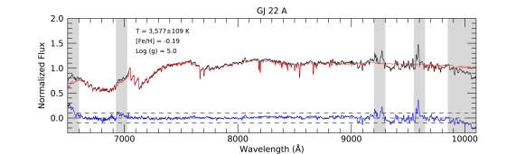
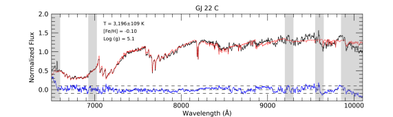
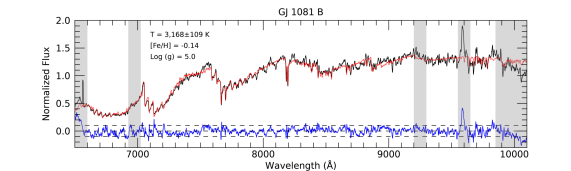
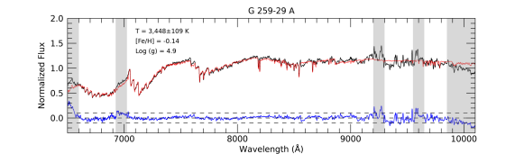
Figure 1: Normalized spectra are plotted in black with the best fitting combination model spectrum over-plotted in red. The shaded gray regions are wavelength ranges not used in the model fit. The fit residual is plotted in blue at the bottom, with the outer dashed lines showing the 10 percent residual mark. Both the observed and the model spectra were smoothed for clarity. High resolution unsmoothed images are available in the electronic version. Fringing is evident as step-like sharp features at wavelengths redder than 9,000 Å.

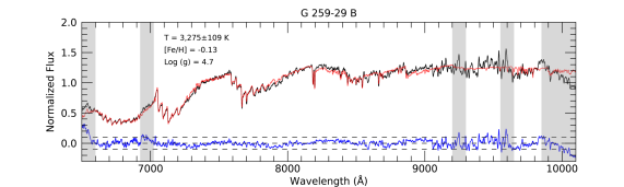
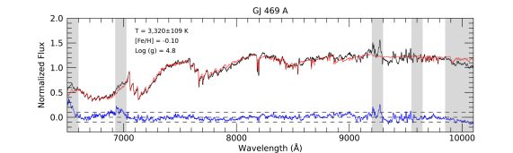
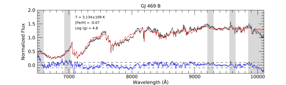
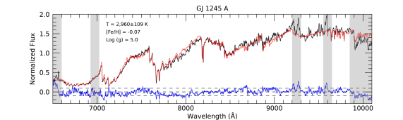
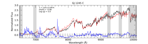
Figure 2: The continuation of Figure 1. The quality of the fits is degraded at lower temperatures, as is evident for GJ 1245 A and C.

We calculated stellar radii in Table 2 by scaling the model flux at the stellar surface and the observed flux via the geometric scaling relation $R_{\star}^{2}=d^{2}(F_{\oplus}/F_{\star})$ where $R_{\star}$ is the stellar radius, $d$ is the trigonometric parallax distance to the star (Table 1), and $F_{\oplus}$ and $F_{\star}$ are the observed flux and the model flux at the stellar surface, respectively. We then calculated luminosities using the Stefan-Boltzmann law and surface gravities based on radii and masses. The latter serve as checks on the surface gravities assumed in the model spectra. We derive the uncertainties in radius in Section 4.1.1 and propagate the uncertainties in temperature and radius to obtain the uncertainties in luminosity.

4.1.1 Validating the Atmospheric Model Fits with Long Baseline Optical Interferometry

To prove the adequacy of our atmospheric model derived quantities (Table 2) we again follow the procedure of Mann et al. (2013). For a calibrator sample of 21 stars we compare effective temperatures and radii against the same quantities derived based on angular diameters directly measured with the CHARA Array long baseline optical inteferometer (Boyajian et al., 2012). Once angular diameters are measured via interferometry stellar radii are trivially obtained given the well known trigonometric parallaxes to these bright nearby stars. Effective temperatures can be calculated via the Stefan-Boltzmann law if the bolometric luminosity is known. The latter can be well approximated thanks to wide photometric and spectroscopic observations covering the spectral energy distribution from the near ultraviolet to the mid infrared. Mann et al. (2013) improved upon the photometric treatment of Boyajian et al. (2012) to derive the interferometric temperatures for the 21 stars listed in Table 3.

Figures 3 and 4 show the comparison of effective temperatures and radii, respectively, obtained with interferometry and our atmospheric model fitting technique. The calibrator spectra from Mann et al. (2013) were kindly made available by Andrew Mann.

The procedure for fitting this sample was the same as the one described in Section 4.1 except that we also excluded the wavelength regions from 7,050 Å to 7,150 Å due to the effect of the atmospheric oxygen A band. All other telluric regions appear to be well accounted for in the spectra of the calibrator stars. We also smoothed the atmospheric models to the considerably lower resolution of the calibrator spectra. The comparison of the effective temperatures obtained with both methods has a standard deviation of 109 K, and we adopt that as the 1$\sigma$ uncertainty in the effective temperatures we derive in this work. Similarly, we adopt a five percent standard deviation in radius. While the temperatures and radii we report in Table 2 overlap with only the cool end of the calibrator sample, inspection of Figures 3 and 4 show no systematic trends. We performed a Student’s t test and found that the effective temperatures derived with interferometry and with atmospheric fits are consistent with belonging to the same sample to 0.89 significance.

We therefore conclude that within the 1$\sigma$ uncertainties we adopt (109 K for effective temperature and five percent for radius) our method is capable of determining the true effective temperature of a sample of stars in a statistical sense. We propagate those uncertainties when using the values in Table 2 to evaluate models of stellar structure and evolution and note that those results (Section 5) should also be viewed as a statistical treatment.

Table 3: Comparison with Interferometric Calibration Sample

Star	Temperature (K)		Radius
	Atm. fit	Interferometry	Atm. fit	Interferometry
GJ 15 A	3631	3602$\pm$13	0.3849	0.3863$\pm$.0021
GJ 105 A	4823	4704$\pm$21	0.7688	0.7949$\pm$.0062
GJ 205	3600	3850$\pm$22	0.6455	0.5735$\pm$.0044
GJ 338 A	4147	3953$\pm$37	0.5326	0.5773$\pm$.0131
GJ 338 B	4048	3926$\pm$37	0.5561	0.5673$\pm$.0137
GJ 380	4019	4176$\pm$19	0.6923	0.6398$\pm$.0046
GJ 412 A	3644	3537$\pm$41	0.3888	0.3982$\pm$.0091
GJ 436	3448	3520$\pm$66	0.4476	0.4546$\pm$.0182
GJ 526	3644	3646$\pm$34	0.5164	0.4840$\pm$.0084
GJ 570 A	4639	4588$\pm$58	0.7286	0.7390$\pm$.0190
GJ 581	3380	3487$\pm$62	0.3256	0.2990$\pm$.0100
GJ 687	3417	3457$\pm$35	0.4317	0.4183$\pm$.0070
GJ 699	3257	3238$\pm$11	0.1926	0.1869$\pm$.0012
GJ 702 B	4305	4475$\pm$33	0.7301	0.6697$\pm$.0089
GJ 725 A	3453	3417$\pm$17	0.3538	0.3561$\pm$.0039
GJ 809	3662	3744$\pm$27	0.5536	0.5472$\pm$.0066
GJ 820 A	4313	4399$\pm$16	0.6867	0.6611$\pm$.0048
GJ 820 B	4052	4025$\pm$24	0.5862	0.6010$\pm$.0072
GJ 880	3613	3731$\pm$16	0.5770	0.5477$\pm$.0048
GJ 887	3691	3695$\pm$35	0.4751	0.4712$\pm$.0086
GJ 892	4734	4773$\pm$20	0.7984	0.7784$\pm$.0053

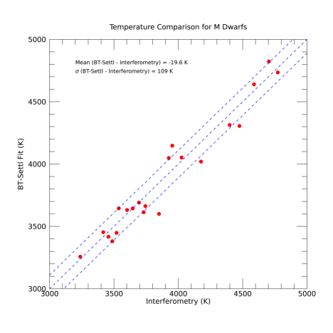
Figure 3: Comparison of effective temperatures obtained with long baseline optical interferometry and our atmospheric fitting technique for a calibrator sample of 21 M dwarfs. The blue dashed lines denote the standard deviation of 109 K. A Student’s t test shows no systematic difference between the samples to 0.89 significance.

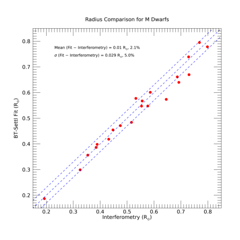
Figure 4: Same as Figure 3, but for comparing radius.

4.1.2 General Considerations Regarding the Atmospheric Fits

As a general trend we note that the BT-Settl spectra provide good fits to the observed data. The quality of the fits is best noted in the digital supplement to Figures 1 and 2, which show the data in its original unsmoothed version. All fits pass the binary metallicity test, where the same range of metallicity must be predicted for the two components of the same binary system, to within about 0.1 dex. The metallicity of two systems, GJ 22 ABC and GJ 1245 ABC is independently known from the isolated B component, and that information can be used as a test on our procedure. Rojas-Ayala et al. (2012) report $[Fe/H]=-0.19$ for GJ 22 B based on infrared spectroscopy. Our procedure finds $[Fe/H]=-0.19$ for GJ 22 A, and $[Fe/H]=-0.10$ for GJ 22 C, thus validating results to no better than 0.1 dex. For GJ 1245 AC Benedict et al. (2016) report $[Fe/H]=-0.04$. We obtain $[Fe/H]=-0.07$ for the A component and $[Fe/H]=-0.08$ for the C component. Despite this agreement, we notice that all 10 stars appear to have slightly sub-solar metallicity in our analysis. This feature could be real or it could be an artifact due to the boundary effect in the metallicity scaling of the model grid. For most temperature and gravity combinations the metallicity ([Fe/H]) ranges from -2.0 to 0.0, with only sporadic coverage up to +0.5. A random linear combination of model spectra (Section 4.1) is therefore likely to be biased towards lower metallicities even if in fact the metallicity is very close to solar. We therefore de-emphasize the absolute scaling of the metallicities in Table 2 and focus on the broad agreement between the metallicities of components of the same system. The models and the data show remarkable fine scale agreement in a line by line basis down to the noise limit, particularly at wavelengths blue than 8,000 Å.

The fits to the gravity sensitive KI doublet at 7,700 Å and NaI doublet at 8,200 Å, and to the TiO bands starting at around 6,650 Å, 7,050 Å, and 7,590 Åare also generally very good. We note, however, that within the limitations of the $Log\,g$ grid spacing there appears to be a slight bias towards calculated surface gravities being higher than the fit values, however without a finer grid it is impossible to determine the significance of this tendency. The mean of the residuals of those fits in the sense of $Log\,g$ derived from the atmospheric fits minus that derived from radius and mass is -0.15. If we exclude the poorly modeled stars GJ 1245 A and C the mean of the residuals becomes -0.09. There is a possibility that this discrepancy is due to the radii derived from atmospheric models being under-estimated. Given the check on the radius methodology from the interferometric data, we believe that such an effect, if present, is small and well within the uncertainties of the derived radii because we see no systematic trends on Figure 4. At the temperatures we consider here surface gravity has little effect on overall spectrum morphology except for altering specific gravity sensitive features such as the KI and NaI lines. When calculating the overall best fit model (Section 4.1) the wavelength coverage of these lines may be too small to meaningfully influence the fit. A direct comparison of the morphology of the KI and NaI doublets between model and spectra may be a better indication of surface gravity, however such comparison would require assumptions in temperature and metallicity. We weighed both approaches and decided to keep the single fit approach because it is a good compromise between diagnosing both effective temperature and surface gravity to reasonable accuracy. We note that the only star with a large discrepancy between the atmospheric model predicted surface gravity and the surface gravity calculated from radius and mass is GJ 1245 C, and in that case the fits to the gravity indicators, particularly the KI doublet, is also poor.

The quality of the fits deteriorates at lower temperatures, as is evident in the fits for GJ 469 B (3,134 K), GJ 1245 A (2,960 K), and particularly GJ 1245 C (2,611 K). The problem could be in part due to the intrinsic difficulty of modeling spectra at cooler temperatures where molecular species and grains become more important, but also due to greater sensitivity to temperature itself. The overall slope of M dwarf spectra increases rapidly as a function of temperature at temperatures $\lesssim$ 3,100 K, and finding a simultaneous fit to the blue and red parts of the spectrum therefore requires a finer grid.

We also note that the depths of individual lines in the red part of the model spectra beyond 8,000 Å  seem to be too shallow while the general shape of the spectrum is still a good match. In other words, the model spectra are smoother than the observed spectra. The fact that we still see a line to line match at the smallest scale, as best seen in the high resolution online supplement to Figures 1 and 2, indicates this discrepancy is not due to noise in the observed spectra. The effect is also distinct from fringing, which is a larger scale feature that tends to alter the spectra in a step-like manner; even within fringed regions, the shallower individual line depths are still present.

Our ability to derive accurate effective temperatures and radii is in large part due to the choice of wavelength region to study, and does not necessarily speak to the adequacy of the BT-Settl models in other wavelength ranges. Even in our case the first 118 Å and the last 277 Å of the observed spectra were omitted from the fit due to considerable deviations between observations and models, as shown in the shaded regions of Figures 1 and 2. The blue region in particular shows residuals of up to 30 percent. It is also well known that incomplete oppacities create problems in the near infrared, particularly in the J band, and that those discrepancies hinder the determination of bolometric flux from model spectra alone. Baraffe et al. (2015) also note that TiO line lists are still incomplete and the incompleteness can cause problems particularly at higher resolutions, however we do not notice higher than usual residuals to TiO bands in Figures 1 and 2. Rajpurohit et al. (2018) also note problems with line widths at higher resolutions, which again do not seem to be problematic at the resolution of this work, as best visualized in the high resolution supplement to Figures 1 and 2. Overall, the red optical and very near infrared region we study here, from 6,600 Å to 9,850 Å, is well modeled in this temperature regime, and the comparison with interferometric results (Section 4.1.1) validates the parameters we derive from atmospheric models, therefore allowing us to use them as the comparison standard for testing models of stellar structure and evolution.

5 Testing Evolutionary Models

Figure 5 shows the distributions of temperatures, luminosities, and radii as functions of mass for the observed sample. An ideal set of evolutionary predictions would be able to replicate these values while respecting the coevality of stars in the same system. Here we focus on five evolutionary model suites that are commonly used to study low mass stars: the Dartmouth models (Dotter et al., 2008), the MIST models (Choi et al., 2016; Dotter, 2016), the models of Baraffe et al. (2015), the PARSEC models (Bressan et al., 2012), and the YaPSI models (Spada et al., 2017).

Figure 5: Temperature, luminosity, and radius as a function of mass for the stars in the sample. Components of the same binary are connected with thin lines and color coded. Panels b and c follow the same color coding as a. Valid evolutionary models must produce isochrones that can replicate these quantities for both components of a given binary simultaneously.

Figures 6, 7, and 8 show evolutionary tracks interpolated to the masses of each star in temperature, luminosity, and radius. Each panel shows the model predictions for the two components of a star system with the results from Table 2 overlaid as shaded regions encompassing the observational constraints from this study. Only the Baraffe et al. (2015) models and the PARSEC models incorporate cool enough atmospheres to model the properties of the coolest star in the study, GJ 1215 C.

Table 4 summarizes the graphical results of Figures 6, 7, and 8 by tabulating the instances in which a given model can accurately predict the observed properties assuming either main sequence ages or pre-main sequence ages. For the purpose of this study we define the zero age main sequence as the point of maximum radius contraction. In Table 4 a fully self-consistent model match in the sense that a model can predict all three fundamental parameters for both stars in a system in a coeval manner is marked with the symbol ✓✓✓. That only happens in the case of the GJ 22 AC system (Section 6.2). The symbols “YY” and “Y” denote when a parameter is correctly modeled if the system is young (pre-main sequence) while respecting or not respecting coevality, respectively. The interpretation of these pre-main sequence matches must be done with caution. From the shape of the evolutionary tracks for luminosity and radius in Figures 6, 7, and 8 it is nearly always possible to find a pre-main sequence solution that falls in the desired parameter space for a short time in the system’s evolution. While we cannot discard these instances as valid matches for pre-main sequence systems, it is unlikely that many of the five star systems we study lie in such a specific narrow range of the pre-main sequence. We note also that none of the systems have a fully self-consistent pre-main sequence solution.

We now discuss topics related to individual model sets and save a general discussion on how well these models work as a whole to Section 7.

5.1 Dartmouth Stellar Evolution Database

The Dartmouth Stellar Evolution Database and its stellar evolution code (Dotter et al., 2008) is an older code that has been periodically updated to provide results in several photometric systems and increase functionality. Its web interface allows for the easy production of isochrones and evolutionary tracks interpolated to any mass, age, and metallicity within their parameter ranges. We used this web interface to produce the results shown in Figures 6, 7, and 8. One particular limitation is that it does not include ages younger than 1 Gyr, and so only main sequence stars can be modeled. This age limitation also excludes the zero age main sequence, as shown most clearly in the radius plots where the other evolutionary models show radius minima.

The Dartmouth models use atmospheric boundary conditions based on the NextGen atmospheric models generated with the PHOENIX radiative transfer code (Hauschildt et al., 1999a, b). These model atmospheres use the older solar abundances of Grevesse & Sauval (1998), which have since been revised several times, as discussed in Allard et al. (2013). Interestingly, this choice of older atmospheric models and older solar metallicities does not seem to drastically affect results when compared to other models. This is in contrast to the effect of using the older solar abundances of Grevesse & Sauval (1998) in atmospheric models, which can cause a noticeable difference in predicted effective temperatures (Mann et al., 2013). We note the wide discrepancy in temperature in the case of GJ 1245 A, where our results show an upper bound on the temperature of 3036 K and the model predicts 3,200 K. A detailed treatment of metallicity becomes more important at lower temperatures as molecular species begin to form and greatly increase the opacity. Therefore, the choice of solar metallicities could be the cause of the temperature discrepancy for GJ 1245 A, which is significantly cooler than the other stars, except for GJ 1245 C.

5.2 MESA Isochrones and Stellar Tracks $-$ MIST

The MIST models (Choi et al., 2016; Dotter, 2016) are an application of the Modular Experiments in Stellar Astronomy (MESA) code that tabulates evolutionary tracks for a wide range of stars using solar-scaled metallicities. The solar metallicity zero points are set to the values adopted in Asplund et al. (2009). MESA is a large, open source comprehensive project that preserves a wide range of freedom in the input parameters for the stellar evolution code, so choosing the adequate parameters for a particular model grid is in itself a complex scientific task.

The evolutionary tracks shown in Figures 6, 7, and 8 were produced using the MIST web interpolator. A feature that readily stand out are what appear to be pulsations, with a period in the order of hundreds of millions of years. No other model shows that behavior. The pulsations are the strongest in the 0.32 M_⊙ to 0.35 M_⊙ mass range, which is close to the mass where stars become fully convective. We discuss issues relating to the onset of full convection in detail in Section 6.4.

One of the distinct advantages of the MESA/MIST approach is the ability to generate new model grids based on different input parameters with relative ease and with minimal knowledge of the inner workings of the code. In that sense it may be possible to produce a different MESA implementation that is calibrated to a narrower set of stars and provides a better match to those observations.

5.3 Models of Baraffe et al., (2015)

The evolutionary models of Baraffe et al. (2015) are the latest in a long tradition of evolutionary models that are not only stellar, but also bridge the stellar-substellar boundary and model the brown dwarf domain. This family of models has incorporated various versions of the PHOENIX model atmospheres as a boundary condition, and this latest installment incorporates the BT-Settl atmospheres used in this work (Sections 4.1 and 4.1.2).

The BT-Settl atmospheric models are arguably the most advanced model atmospheres used as a boundary condition for any of the evolutionary models we studied. Further, the fact that the Baraffe et al. (2015) models incorporate the same atmospheres we used to derive fundamental parameters leads us to expect a somewhat better agreement between those parameters and the model predictions. Yet, their results are mixed and not qualitatively better than the models that use other atmospheric boundary conditions (Dartmouth and MIST). The same can be said for the YaPSI models, which also incorporate the BT-Settl atmospheres. This consideration again suggests that any mismatches may be indicative of deeper theoretical discrepancies independent of the choice of atmospheric boundary conditions.

One advantage of the Baraffe et al. (2015) models is that they include significantly lower temperatures, and along with PARSEC are the only models discussed here that can model GJ 1245 C at 2,611$\pm$109 K. However as seen in Figure 8, the temperature predictions would only agree to the inferred value if the GJ 1245 system is young, with an age ranging from 250 Myr to 800 Myr, and that would then be in disagreement with the predictions for luminosity. While both components of GJ 1245 exhibit H$\alpha$ emission (Figure 2, best seen in the high resolution digital supplement) such emission is common in this very low mass regime (note also H$\alpha$ emission in GJ 22 C and GJ 1081 B), and does not necessarily indicate youth (e.g., Browning et al., 2010).

5.4 The PARSEC Models

The PAdova-TRieste Stellar Evolution Code (Bressan et al., 2012) is a versatile family of codes that over the years has developed specific treatments for different regions of the HR diagram. Chen et al. (2014) updated the code for the specific treatment of the lower main sequence. The code allows the choice of a wide range of parameters including a well populated metallicity grid and has a convenient web interface. The code uses the BT-Settl atmospheres (Section 4.1) as the boundary condition, albeit with the older metallicities of Asplund et al. (2009). Chen et al. (2014) calibrates the model using the main sequences of several young and intermediate age star clusters, and obtains remarkably good results from a populations perspective in the sense that their isochrones are a good representation of the cluster’s main sequence. However in such a comparison masses are treated indirectly in the sense that unless the cluster’s initial mass function is precisely known mass becomes a free parameter for the color-magnitude fit. When masses become a fixed parameter we find that the PARSEC models are systematically too cold. Their temperatures tend to be about 200 K to 300 K lower than our inferred temperatures, as shown in the top panels of Figures 6, 7, and 8. While their radius predictions are in range with the other models, the predicted luminosities are accordingly lower. We note however that if these mismatches could be fixed while preserving PARSEC’s ability to model populations in the HR diagram it would become a powerful tool.

5.5 The YaPSI Models

The Yale-Postdam Stellar Isochrones (YaPSI, Spada et al., 2017) are an adaptation of the Yonsei-Yale family of codes modified to emphasize the physics of low mass stars. Their approach also relies on BT-Settl boundary conditions. Tow distinguishing factors are an extremely fine mass grid and the availability of a Markov Chain Monte Carlo grid interpolator available for download. The ability to do fine grid interpolation is useful when testing boundary cases, such as the transition to full convection (Section 6.4). The authors tested the YaPSI models using the mass-luminosity relation of Benedict et al. (2016) (Section 2), the predecessor to our study that provided the dynamical masses we use here. Benedict et al. provide only $V$ and $K$ magnitudes for individual components, as opposed to the fundamental parameters we provide here. Spada et al. (2017) show that the YaPSI models as an ensemble do a good job of replicating the color-magnitude diagram of Benedict et al. (2016), albeit with wide dispersion about the model sequence. Our tests show that the YaPSI models do comparatively well. Table 4 shows that the YaPSI models do a slightly better job than the other models in predicting the parameters of individual stars, however they still lack the self-consistency necessary to fully match systems other than GJ 22. One drawback is that their lower mass limit is 0.15 M_⊙, and so they cannot model GJ 1245 A and C.

Figure 6: Evolutionary plots for the GJ 22 (left column) and GJ 1081 (right column) systems. The line style and color scheme is as follows: solid red line for Dartmouth plots, solid blue line for MIST plots, blue dotted lines for the Baraffe models, red dotted lines for the PARSEC models, and green dashed lines for the YaPSI models. Two tracks are shown for each model, corresponding to the primary and secondary components. The shaded areas show the uncertainties inferred from the atmospheric fits (Table 2)See Section 6.2 for a discussion of the metallicity of GJ 22 AC.

Figure 7: Same as Figure 6 for the G 250-29 and GJ 469 systems.

Figure 8: Same as Figure 6 for the GJ 1245 system. Only the Baraffe (blue dotted lines) and the PARSEC (red dotted lines) models reach cool enough temperatures to model GJ 1245 C.

6 Discussion

With the exception of the PARSEC models most of the evolutionary tracks shown in Figures 6, 7, and 8 could be reconciled with the BT-Settl predictions (Table 2) if the uncertainties in temperature were increased by an additional 50 K on each side and if uncertainties in radius were about doubled. In that sense it may well be that our expectations of evolutionary models are simply higher than what is possible, and we should conform to temperature predictions no more accurate than 300 K. That realization would be unfortunate because M dwarf effective temperatures and radii are routinely expressed to much smaller uncertainties (e.g., Dieterich et al., 2014; Mann et al., 2015) and as discussed in Section 4.1.1 can indeed be determined to better precision.

6.1 Radius Inflation

Several observational studies that measure M dwarf radii using eclipsing binaries or optical interferometry indicate that the radii of M dwarfs tend to be larger than those predicted by stellar structure models (e.g., Torres et al., 2010; Boyajian et al., 2012; Feiden & Chaboyer, 2012). This trend is the so called radius inflation problem. Most hypothesized explanations for the discrepancy involve the interaction of magnetic fields with stellar matter. We find that radius inflation is indeed a significant problem, with more than half of model predictions resulting in radii that are two small, as shown in Table 5. We find only three instances of a radius being over predicted, and those involve the GJ 1245 AC system, which has proven more difficult to model due to its very low mass.

Inspection of Figures 6, 7, and 8 and Table 4 shows that radius inflation is the leading reason why model predictions do not achieve the desired self-consistent solutions for binary systems other than GJ 22. None of the models we test here include the effects of magnetism. If radius inflation is indeed due to magnetic effects that would provide a natural explanation of the problem.

6.2 GJ 22 AC, A Well Behaved Metal Poor System?

Out of the five star systems we used to test models the GJ 22 AC system stands out as the only system for which the models of stellar structure and evolution were able to produce an accurate and self consistent solution. This is true of all models except for the PARSEC model, which has systematic problems with under predicting effective temperatures (Section 5.4). As discussed in Section 4.1.2, the GJ 22 system is known to be slightly metal poor, with Rojas-Ayala et al. (2012) finding $[Fe/H]=-0.19$, in agreement with our model fit. The system can therefore be used as a model for the effect of deviations in metallicity for stars with known masses. Out of the five evolutionary models we consider in this work three have fine enough metallicity grids to model the effect of of a change in metallicity of -0.19 dex. These are the Dartmouth models, the MESA/MIST models, and the PARSEC models (Sections 5.1, 5.2, and 5.4, respectively). Figure 6 shows these three models plotted with $[Fe/H]=-0.20$ while the models of Baraffe et al. (2015) and the YaPSI models remain at solar metallicity. Figure 9 shows the evolutionary tracks of the three models that encompass lower metallicities plotted at both solar metallicity and $[Fe/H]=-0.20$. For a given mass there is an increase in temperature and a corresponding increase in luminosity, while radius remains mostly unchanged for main sequence ages. The variations due to this small change in metallicity appear to be contained within the uncertainties of the atmospheric models. Not counting the PARSEC models, Figures 6 and 9 show equally acceptable fits for both solar metallicity models and the models with reduced metallicity. The cause of the good evolutionary fits to GJ 22 A and C therefore appears to not be connected to any variation in metallicity, which could have been indicative of problems with the solar zero points adopted by the several different models.

Our data do not support any further explanation for the fact that the models provide such a good match to the GJ 22 AC system. We note that while the spectroscopic fits GJ 22 A and C are good, so are the ones for other stars in the sample. GJ 22 C also exhibits strong H$\alpha$ emission, as is common for mid to late M dwarfs, so a lack of magnetic activity cannot be invoked as a simplifying factor either. Another possible explanation is that in joint light $V\,sin\,i<4\,km/s$ for GJ 22 AC, indicating that both components are slow rotators (Reiners et al., 2012).

We suggest that further comparative studies between the GJ 22 AC system and other systems could be particularly instructive with regards to what is and is not working in stellar models.

Figure 9: Evolutionary tracks for GJ 22 A and C for models that vary metallicity. The dotted lines indicate solar metallicity while the solid lines indicate $[Fe/H]=-0.2$ to approximate the metallicity of the GJ 22 system ($[Fe/H]=-0.19$). Blue lines represent the MESA/MIST models, red lines represent the Dartmouth models, and green lines show the PARSEC models. At main sequence ages radius remains nearly invariant while temperature and luminosity increase with decreasing metallicity. The shaded areas show the uncertainties inferred from the atmospheric fits (Table 2). Both metallicities can be accommodated by the data.

6.3 G 250-29 B and GJ 469 B: The Effects of Small Changes in Mass and Metallicity

G 250-29 B and GJ 469 B provide an interesting example of how stars with very similar masses and metallicities can vary significantly in luminosity and temperature. Figure 10 shows the spectra for G 250-29 B (0.187$\pm$0.004 M_⊙) and GJ 469 B (0.188$\pm$0.004 M_⊙). While the spectra are remarkably similar in morphology the spectrum of G 250-29 B has about 1.5 times the flux of GJ 469 B. Using the atmospheric derivations listed in Table 2, G 250-29 B is more luminous by a factor of 1.26, still within the uncertainties, and hotter by 145 K, which is significant given the uncertainty in temperature of 109 K (Section 4.1.1). Their radii are also significantly different at 0.231$\pm$0.011 R_⊙ for G 250-29 B and 0.266$\pm$0.011 R_⊙ for GJ 469 B. Neither system shows signs of youth, with no H$\alpha$ emission, calculated $Log\,g=5.0$, and well fit Ca and K gravity indicators. There may be a slight difference in metallicity, with metallicities ([Fe/H]) of -0.14 and -0.11 for the A and B components of G 250-29 B, respectively, and -0.10 and -0.07 for the A and B components of GJ 469. These differences are only borderline in significance given that we can only infer the equal metallicities of components of the same binaries to about 0.1 dex, however they do work in the conventional sense of making the most metal poor stars hotter. In the case of the GJ 22 system we saw that a significantly greater difference in metallicity of -0.19 had the effect of changing the predicted model temperatures by only about 100 K (Figure 9), therefore either the models are unreliable in their treatment of metallicity or it is unlikely that such a small change in metallicity between G 250-29 B and GJ 469 B would account for such a large change in observable characteristics.

This comparison between G 250-29 B and GJ 469 B shows that even with very similar masses measured to high precision two stars can be significantly different. The reasons for these differences are not clear, and that adds a note of caution when interpreting M dwarf evolutionary models. There are still higher order effects that probably cannot be understood given our current constraints on observational parameters and our ability to model them.

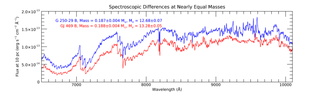
Figure 10: Flux calibrated spectra for G 250-29 B and GJ469 B. The spectra were smoothed using a Gaussian kernel for clarity. G 250-29 B has about 1.5 times the flux of GJ 469 B. Fringing is present at wavelengths greater than 9,000 Å.

6.4 The Transition to Full Convection, the Jao Gap, and the Convective Kissing Instability

The transition to a fully convective interior is a hallmark of M dwarfs. It is predicted to occur at masses ranging from 0.28 M_⊙ to 0.33 M_⊙ (e.g., Chabrier & Baraffe, 1997), corresponding to early to mid M subtypes. Since then several works have attempted to refine our understanding of this transition. Understanding this transition has become particularly interesting in light of the so called Jao gap (Jao et al., 2018), a thin gap in the color-magnitude diagram noticed in Gaia DR2 data that is thought to be related to the transition to full convection.

Theoretical work by van Saders & Pinsonneault (2012) propose that there exists a mass range immediately above the onset of full convection where ³He burning produces a convective core that is initially separated from the star’s deep convective zone by a thin radiative envelope. As the convective core grows, periodic merging with the convective envelope causes pulsations in luminosity, temperature, and radius. They call this phenomenon the convective kissing instability. Their work uses the MESA stellar evolution code (Section 5.2) The MIST evolutionary tracks plotted in Figures 6 and 7 show those oscillations for three stars: G 250-29 A (0.35 M_⊙), GJ 469 A (0.33 M_⊙), and GJ 1081 A (0.32 M_⊙). Baraffe & Chabrier (2018) also note the existence of the convective kissing instability, but at a much narrower mass range of 0.34 M_⊙ to 0.36 M_⊙. While that work predicts pulsations, they do not appear in the Baraffe et al. (2015) evolutionary tracks for G 250-29 A (0.35 M_⊙, Figure 7) because that work produced a model grid in steps of 0.1 M_⊙ as opposed to 0.01 M_⊙ in Baraffe & Chabrier (2018). Our interpolation therefore skipped over this feature. MacDonald & Gizis (2018) also postulate that the Jao gap is caused by the increase in luminosity due to the merging of a convective core and a convective envelope originally separated by a thin radiative zone, but do not find that this merging leads to a periodic instability. As discussed extensively in Jao et al. (2018), the YaPSI models (Section 5.5) predict the Jao gap even though we do not see any manifestation of pulsations in the YaPSI plots in this work. Without finer mass coverage it is impossible to generalize the discussion to other models, and a general assessment of issues regarding the convective kissing instability or other features that may be causing the Jao gap is not our goal. Our intent here is only to note an interesting feature that we saw in a model set (the MIST models) in light of a recent discovery (the Jao gap), and provide some context.

As seen in the above discussion, several theoretical issues with observational implications arise in the mass range bordering the transition from partial to full convection. It would be interesting to test whether or not the convective kissing instability exists by detecting a relation in fundamental parameters that follows the pulsations predicted by the MIST models for G 250-29 A, GJ 469 A, and GJ 1081 A. Similarly, the steeper slope of the mass luminosity relation around the transition to full convection predicted by the YaPSI models should be tested observationally. While the dynamical masses in our data set are precise enough, we lack the very large sample with finely spaced mass coverage that would be required for such tests. We therefore emphasize that even with the robust mass-luminosity relation of Benedict et al. (2016) there are still open questions in low mass stellar structure whose answers will require the study of many more systems with dynamical masses.

Table 4: Model Matches

Star, Property	MIST	Dartmouth	Bar. 2015	PARSEC	YaPSI
GJ 22 A $T_{eff}$	✓✓✓	✓✓✓	✓✓✓	X	✓✓✓
$L$	✓✓✓	✓✓✓	✓✓✓	✓Y	✓✓✓
$R$	✓✓✓	✓✓✓	✓✓✓	✓✓	✓✓✓
GJ 22 C $T_{eff}$	✓✓✓	✓✓✓	✓✓✓	X	✓✓✓
$L$	✓✓✓	✓✓✓	✓✓✓	YY	✓✓✓
$R$	✓✓✓	✓✓✓	✓✓✓	✓✓	✓✓✓
GJ 1081 A $T_{eff}$	✓✓	✓✓	✓✓	X	✓✓
$L$	✓✓	✓✓	✓✓	YY	✓✓
$R$	X	X	YY	✓✓	✓
GJ 1081 B $T_{eff}$	✓✓	✓✓	✓✓	X	✓✓
$L$	✓✓	✓✓	✓✓	YY	✓✓
$R$	X	X	YY	✓✓	✓
G 250-29 A $T_{eff}$	✓✓	✓✓	✓✓	X	✓✓
$L$	✓Y	✓	✓Y	YY	✓✓
$R$	Y	✓	✓Y	✓Y	✓Y
G 250-29 B $T_{eff}$	✓✓	✓✓	✓✓	X	✓✓
$L$	YY	X	Y	YY	✓✓
$R$	Y	X	YY	Y	YY
GJ 469 A $T_{eff}$	X	✓	X	✓	✓✓
$L$	✓✓	✓✓	✓Y	✓Y	✓✓
$R$	✓Y	✓Y	✓Y	✓✓	✓Y
GJ 469 B $T_{eff}$	✓	X	✓	X	✓✓
$L$	✓✓	✓✓	YY	YY	✓✓
$R$	Y	YY	YY	✓✓	YY
GJ 1245 A $T_{eff}$	✓	X	✓	X	$\cdots$
$L$	✓	X	✓✓	✓	$\cdots$
$R$	✓	✓	✓	X	$\cdots$
GJ 1245 C $T_{eff}$	$\cdots$	$\cdots$	Y	X	$\cdots$
$L$	$\cdots$	$\cdots$	✓✓	✓✓	$\cdots$
$R$	$\cdots$	$\cdots$	X	X	$\cdots$

Table 5: Radius Comparisons

Star, Property	MIST	Dartmouth	Bar. 2015	PARSEC	Yapsi
GJ 22 A	✓	✓	✓	✓	✓
C	✓	✓	✓	✓	✓
GJ 1081 A	$\Uparrow$	$\Uparrow$	$\Uparrow$	$\Uparrow$	$\Uparrow$
B	$\Uparrow$	$\Uparrow$	$\Uparrow$	✓	$\Uparrow$
G 259-29 A	$\Uparrow$	✓	$\Uparrow$	✓	✓
B	$\Uparrow$	$\Uparrow$	$\Uparrow$	$\Uparrow$	$\Uparrow$
GJ 469 A	✓	✓	✓	✓	✓
B	$\Uparrow$	$\Uparrow$	$\Uparrow$	✓	$\Uparrow$
GJ 1245 A	✓	✓	✓	$\Downarrow$	$\cdots$
C	$\cdots$	$\cdots$	$\Downarrow$	$\Downarrow$	$\cdots$

6.5 Other Models

In the current study we test the hypothesis that evolutionary models can produce model grids applicable to a wide range of stellar masses, and obtained mixed results. One limitation of the grid approach is that it becomes difficult to treat second order effects such as rotation and magnetism. It is particularly noteworthy than none of the models discussed in Section 5 include magnetism.

It is not our goal here to judge the merits of models we did not include in our tests, however it is worth noting that other approaches to stellar modeling exist, and that many of them attempt to model the effects of magnetism, rotation, and other higher order factors. Significant work has been done in extending conventional models into the magnetic domain with the incorporation of magnetohydrodynamics, with emphasis on its effects on convection and radius inflation (e.g., Feiden & Chaboyer, 2012; Mullan & MacDonald, 2001). These models are usually tested on a small number of stars with well known properties. Examples of low mass stars for which these models were applied are: KOI-126 (Feiden et al., 2011; Spada & Demarque, 2012), EF Aquarii (Feiden & Chaboyer, 2012), UV PSc, YY Gem, and CU Cnc (Feiden & Chaboyer, 2013), Kepler-16 and CM Dra (Feiden & Chaboyer, 2014), UScoCTIO5 and HIP 78977 (Feiden, 2016), LSPM J1314+1320 (MacDonald & Mullan, 2017a), LP 661-13, KELT J041621-620046, and AD 3814 (MacDonald & Mullan, 2017b), GJ 65 A (MacDonald et al., 2018), and Trappist-1 (Mullan et al., 2018).

Unfortunately few of these tests used stars with well measured dynamical masses, so the fundamental connection between mass and stellar evolution is often tested only indirectly. Due to the work we present here the field is now ripe for a new generation of model testing when theorists can use this data set to fine tune model predictions.

7 Conclusions and Future Work

The results from our tests are mixed. On one perspective, it is clear that, with the exception of GJ 22 AC, the models cannot provide fully consistent solutions to the full extent of the binary star evolution test. From another perspective, the conditions of this test are quite stringent, and we should not dismiss the fact that the models do have predictive power. It is also important to keep in mind that the tests must be interpreted on a statistical context because while models themselves are theoretical and do not carry uncertainties, their comparisons to data do. The data we are testing against, namely the matches between observed spectra and model atmospheres summarized in Table 2 are matches that as an ensemble carry an uncertainty, quoted and propagated to 1 $\sigma$. Because those atmospheric model comparisons are the root for evolutionary model comparisons and they have been validated to 1 $\sigma$ to the quoted uncertainties we should expect the comparisons, or predictions, made by the evolutionary models to also be correct only two thirds of the time, regardless of the fact that models themselves are not constructed to a certain level of uncertainty. We should further take into account that, despite the significant amount of observing resources used by this project, the test sample remains small. A sample of ten stars in five binary systems is prone to uncertainties arising from statistics of small numbers. Nevertheless, being in full agreement with the data only in one out of five systems is likely to be a deficit beyond statistical uncertainties. As previously noted, agreement between models and observations could be reached if the uncertainties in the quantities derived from atmospheric models were artificially increased. In that sense it is clear that atmospheric models are further along in predictive power than evolutionary models when it comes to predicting the same basic stellar parameters. On the other hand, analysis of the similarities and differences between G 250-29 B and GJ 469 B (Section 6.3) indicates that the problem of M dwarf modeling may be intrinsically more complex than what we imagine, with stars of similar masses and metallicities having significantly different observable parameters. If that is a general case then it could be that the expectation we have for model results are simply not realistic.

We believe that the best way to interpret the results we present here is to say that evolutionary models should be used with caution. In an age when the drive to characterize exoplanets places a large emphasis on stellar parameters, the accuracy of parameters derived from evolutionary models should not yet be taken for granted, as they often are.

We believe, however, that the true value of the data we present here is its potential to test models that are specifically built or fine-tuned to the dynamical masses and spectra of each binary component, while respecting the constraints of coevality and equal metallicity natural to a binary system. As such, we see these observations and the present work not only as a means to test the past, but rather as a tool to guide future theoretical efforts. We note that all spectra discussed here are available as a digital supplement to this work and we encourage theorists to use them as a means of constraining new models.

On the observational front we note the need of similar observations to extend the mass coverage to the late M dwarfs, where our analysis was based on only one binary system, GJ 1245 AC. We note also that while broad mass coverage is valuable, detailed observations of systems of nearly equal mass with well known dynamical masses are essential to make sense of secondary effects such as rotation and magnetic field topology, especially around the transition to full convection. We plan to carry out similar observations for such systems in the near future.

8 Summary

We used HST/STIS to obtain spatially resolved spectra of five M dwarf systems with known individual dynamical masses and used them as benchmarks to test models of stellar structure and evolution. Our principal findings are as follows.

• The BT-Settl atmospheric models produce synthetic spectra that are a good match to observations, and their validity was verified by comparison to parameters derived with long baseline optical interferometry (Section 4.1.1). We adopt their best match temperature as an approximation of the true effective temperature of our targets. The agreement is somewhat worse at cooler temperatures, possibly due to the need for a finer temperature grid and also the intrinsic complexity in modeling cooler atmospheres due to molecules and dust formation (Section 4.1.2).

• There may be a weak tendency for the BT-Settl models to underestimate surface gravities (Section 4.1.2).

• We tested the Dartmouth evolutionary models (Dotter et al., 2008), the MIST evolutionary models (Choi et al., 2016; Dotter, 2016), the models of Baraffe et al. (2015), the PARSEC models (Bressan et al., 2012), and the YaPSI models (Spada et al., 2017) with the properties derived from our comparison of observed spectra to model atmospheres. We find only marginal agreement between evolutionary models and observations. Out of five systems the models only reproduced one of them, GJ 22 AC, in a self consistent manner. We note that the PARSEC models are systematically too cold (Section 5, Figures 6, 7, and 8, and Table 4).

• We confirm the known tendency towards radius inflation, in the sense that models under-predict the true radius (Section 6.1).

• We note that the GJ 22 AC system is well modeled in a self-consistent manner by all models we tested except for the systematically too cold PARSEC models. The system is slightly metal poor, but that does not seem to affect the quality of the fits. It is not clear what if anything is special about the GJ 22 system (Section 6.2).

• We discuss the case of G 250-29 B and GJ 469 B, where nearly equal masses and metallicities produce significantly different luminosities, temperature and radii. This example may be indicative of the need for a more detailed treatment of stellar structure and evolution (Section 6.3).

• We note that the principal utility of the data presented here is not as a test of existing models but rather as a guide for future theoretical approaches. As such, we include all data as a digital supplement (Section 7).

• We emphasize the need for more spatially resolved spectroscopic observations of M dwarfs with dynamical masses, especially for masses close to the transition to full convection (Section 6.4 and for late M dwarfs, where our coverage consists of a single system, GJ 1245 AC (Section 7).

References

- Allard et al. (2013) Allard, F., Homeier, D., Freytag, B., Schaffenberger, W., & Rajpurohit, A. S. 2013, ArXiv e-prints, arXiv:1302.6559
- Allard et al. (2012) Allard, F., Homeier, D., Freytag, B., & Sharp, C. M. 2012, in EAS Publications Series, Vol. 57, EAS Publications Series, ed. C. Reylé, C. Charbonnel, & M. Schultheis, 3–43
- Asplund et al. (2009) Asplund, M., Grevesse, N., Sauval, A. J., & Scott, P. 2009, ARA&A, 47, 481
- Baraffe & Chabrier (2018) Baraffe, I., & Chabrier, G. 2018, A&A, 619, A177
- Baraffe et al. (2015) Baraffe, I., Homeier, D., Allard, F., & Chabrier, G. 2015, A&A, 577, A42
- Benedict et al. (2016) Benedict, G. F., Henry, T. J., Franz, O. G., et al. 2016, AJ, 152, 141
- Bochanski et al. (2007) Bochanski, J. J., West, A. A., Hawley, S. L., & Covey, K. R. 2007, AJ, 133, 531
- Boeshaar (1976) Boeshaar, P. C. 1976, PhD thesis, Ohio State University, Columbus.
- Bostroem & Proffitt (2011) Bostroem, K. A., & Proffitt, C. 2011, STIS Data Handbook v. 6.0
- Boyajian et al. (2012) Boyajian, T. S., von Braun, K., van Belle, G., et al. 2012, ApJ, 757, 112
- Bressan et al. (2012) Bressan, A., Marigo, P., Girardi, L., et al. 2012, MNRAS, 427, 127
- Browning et al. (2010) Browning, M. K., Basri, G., Marcy, G. W., West, A. A., & Zhang, J. 2010, AJ, 139, 504
- Caffau et al. (2011) Caffau, E., Ludwig, H.-G., Steffen, M., Freytag, B., & Bonifacio, P. 2011, Sol. Phys., 268, 255
- Chabrier & Baraffe (1997) Chabrier, G., & Baraffe, I. 1997, A&A, 327, 1039
- Chen et al. (2014) Chen, Y., Girardi, L., Bressan, A., et al. 2014, MNRAS, 444, 2525
- Choi et al. (2016) Choi, J., Dotter, A., Conroy, C., et al. 2016, ApJ, 823, 102
- Cushing et al. (2008) Cushing, M. C., Marley, M. S., Saumon, D., et al. 2008, ApJ, 678, 1372
- Delfosse et al. (2000) Delfosse, X., Forveille, T., Ségransan, D., et al. 2000, A&A, 364, 217
- Dieterich et al. (2014) Dieterich, S. B., Henry, T. J., Jao, W.-C., et al. 2014, AJ, 147, 94
- Dotter (2016) Dotter, A. 2016, ApJS, 222, 8
- Dotter et al. (2008) Dotter, A., Chaboyer, B., Jevremović, D., et al. 2008, ApJS, 178, 89
- Feiden (2016) Feiden, G. A. 2016, A&A, 593, A99
- Feiden & Chaboyer (2012) Feiden, G. A., & Chaboyer, B. 2012, ApJ, 761, 30
- Feiden & Chaboyer (2013) —. 2013, ApJ, 779, 183
- Feiden & Chaboyer (2014) —. 2014, ApJ, 789, 53
- Feiden et al. (2011) Feiden, G. A., Chaboyer, B., & Dotter, A. 2011, ApJ, 740, L25
- Gaia Collaboration et al. (2018) Gaia Collaboration, Brown, A. G. A., Vallenari, A., et al. 2018, ArXiv e-prints, arXiv:1804.09365
- Goudfrooij et al. (1998) Goudfrooij, P., Bohlin, R. C., Walsh, J. R., & Baum, S. A. 1998, STIS Near-IR Fringing. II. Basics and Use of Contemporaneous Flats for Spectroscopy of Point Sources (Rev. A), Tech. rep.
- Goudfrooij & Christensen (1998) Goudfrooij, P., & Christensen, J. A. 1998, STIS Near-IR Fringing. III. A Tutorial on the Use of the IRAF Tasks, Tech. rep.
- Grevesse & Sauval (1998) Grevesse, N., & Sauval, A. J. 1998, Space Sci. Rev., 85, 161
- Hauschildt et al. (1999a) Hauschildt, P. H., Allard, F., & Baron, E. 1999a, ApJ, 512, 377
- Hauschildt et al. (1999b) Hauschildt, P. H., Allard, F., Ferguson, J., Baron, E., & Alexander, D. R. 1999b, ApJ, 525, 871
- Hauschildt et al. (1997) Hauschildt, P. H., Baron, E., & Allard, F. 1997, ApJ, 483, 390
- Henry et al. (1999) Henry, T. J., Franz, O. G., Wasserman, L. H., et al. 1999, ApJ, 512, 864
- Henry & McCarthy (1993) Henry, T. J., & McCarthy, Jr., D. W. 1993, AJ, 106, 773
- Jao et al. (2018) Jao, W.-C., Henry, T. J., Gies, D. R., & Hambly, N. C. 2018, ApJ, 861, L11
- Krist et al. (2011) Krist, J. E., Hook, R. N., & Stoehr, F. 2011, in Proc. SPIE, Vol. 8127, Optical Modeling and Performance Predictions V, 81270J
- Limber (1958) Limber, D. N. 1958, ApJ, 127, 363
- MacDonald & Gizis (2018) MacDonald, J., & Gizis, J. 2018, MNRAS, 480, 1711
- MacDonald & Mullan (2017a) MacDonald, J., & Mullan, D. J. 2017a, ApJ, 843, 142
- MacDonald & Mullan (2017b) —. 2017b, ApJ, 850, 58
- MacDonald et al. (2018) MacDonald, J., Mullan, D. J., & Dieterich, S. 2018, ApJ, 860, 15
- Mann et al. (2015) Mann, A. W., Feiden, G. A., Gaidos, E., Boyajian, T., & von Braun, K. 2015, ApJ, 804, 64
- Mann et al. (2013) Mann, A. W., Gaidos, E., & Ansdell, M. 2013, ApJ, 779, 188
- Mould (1976) Mould, J. R. 1976, A&A, 48, 443
- Mullan & MacDonald (2001) Mullan, D. J., & MacDonald, J. 2001, ApJ, 559, 353
- Mullan et al. (2018) Mullan, D. J., MacDonald, J., Dieterich, S., & Fausey, H. 2018, ApJ, 869, 149
- Osterbrock (1953) Osterbrock, D. E. 1953, ApJ, 118, 529
- Rajpurohit et al. (2018) Rajpurohit, A. S., Allard, F., Rajpurohit, S., et al. 2018, A&A, 620, A180
- Reiners et al. (2012) Reiners, A., Joshi, N., & Goldman, B. 2012, AJ, 143, 93
- Rojas-Ayala et al. (2012) Rojas-Ayala, B., Covey, K. R., Muirhead, P. S., & Lloyd, J. P. 2012, ApJ, 748, 93
- Skrutskie et al. (2006) Skrutskie, M. F., Cutri, R. M., Stiening, R., et al. 2006, AJ, 131, 1163
- Spada & Demarque (2012) Spada, F., & Demarque, P. 2012, MNRAS, 422, 2255
- Spada et al. (2017) Spada, F., Demarque, P., Kim, Y. C., Boyajian, T. S., & Brewer, J. M. 2017, ApJ, 838, 161
- Torres et al. (2010) Torres, G., Andersen, J., & Giménez, A. 2010, A&A Rev., 18, 67
- van Saders & Pinsonneault (2012) van Saders, J. L., & Pinsonneault, M. H. 2012, ApJ, 751, 98
- Vrijmoet et al. (2020) Vrijmoet, E. H., Henry, T. J., Jao, W.-C., & Dieterich, S. B. 2020, AJ, 160, 215
- York et al. (2000) York, D. G., Adelman, J., Anderson, Jr., J. E., et al. 2000, AJ, 120, 1579