Evaluating Explanations: How much do explanations
from the teacher aid students?

Abstract

While many methods purport to explain predictions by highlighting salient features, what aims these explanations serve and how they ought to be evaluated often go unstated. In this work, we introduce a framework to quantify the value of explanations via the accuracy gains that they confer on a student model trained to simulate a teacher model. Crucially, the explanations are available to the student during training, but are not available at test time. Compared to prior proposals, our approach is less easily gamed, enabling principled, automatic, model-agnostic evaluation of attributions. Using our framework, we compare numerous attribution methods for text classification and question answering, and observe quantitative differences that are consistent (to a moderate to high degree) across different student model architectures and learning strategies.

1 Introduction

The success of deep learning models, together with the difficulty of understanding how they work, has inspired a subfield of research on explaining predictions, often by highlighting specific input features deemed somehow important to a prediction Ribeiro et al. (2016); Sundararajan et al. (2017); Shrikumar et al. (2017). For instance, we might expect such a method to highlight spans like “poorly acted” and “slow-moving” to explain a prediction of negative sentiment for a given movie review. However, there is little agreement in the literature as to what constitutes a good explanation Lipton (2016); Jacovi and Goldberg (2021). Moreover, various popular methods for generating such attributions disagree considerably over which tokens to highlight (Table 1). With so many methods claimed to confer the same property while disagreeing so markedly, one path forward is to develop clear quantitative criteria for evaluating purported explanations at scale.

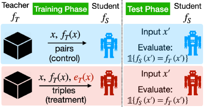
Figure 1: The proposed framework for quantifying explanation quality. Student models learn to mimic the teacher, with and without explanations (provided as “side information” with each example). Explanations are effective if they help students to better approximate the teacher on unseen examples for which explanations are not available. Students and teachers could be either models or people.

The status quo for evaluating so-called explanations skews qualitative—many proposed techniques are evaluated only via visual inspection of a few examples Simonyan et al. (2014); Sundararajan et al. (2017); Shrikumar et al. (2017). While several quantitative evaluation techniques have recently been proposed, many of these are easily gamed (Treviso and Martins, 2020; Hase et al., 2020). Some depend upon the model outputs corresponding to deformed examples that lie outside the support of the training distribution DeYoung et al. (2020), and a few validate explanations on specifically crafted tasks Poerner et al. (2018).

	Random	Grad Norm	Grad $\times$ Inp	LIME	DeepLIFT	Layer Cond.	Integrated Gradients	Attention
Random	1.00	0.10	0.10	0.10	0.10	0.10	0.10	0.10
Grad Norm	0.10	1.00	0.27	0.13	0.22	0.19	0.22	0.30
Grad$\times$Inp	0.10	0.27	1.00	0.11	0.28	0.14	0.16	0.17
LIME	0.10	0.13	0.11	1.00	0.11	0.16	0.16	0.15
DeepLIFT	0.10	0.22	0.28	0.11	1.00	0.18	0.23	0.25
Layer Cond.	0.10	0.19	0.14	0.16	0.18	1.00	0.49	0.22
Integrated Gradients	0.10	0.22	0.16	0.16	0.23	0.49	1.00	0.24
Attention	0.10	0.30	0.17	0.15	0.25	0.22	0.24	1.00

Table 1: Overlap among the top-$10\%$ tokens selected by different explanation techniques for sentiment analysis. In each row, for a given technique, we tabulate the fraction of explanatory tokens that overlap with other explanations. Value of 1.0 implies perfect overlap and 0.0 denotes no overlap.

In this work, we propose a new framework, where explanations are quantified by the degree to which they help a student model in learning to simulate the teacher on future examples (Figure 1). Our framework addresses a coherent goal, is model-agnostic and broadly applicable across tasks, and (when instantiated with models as students) can easily be automated and scaled. Our method is inspired by argumentative models for justifying human reasoning, which posit that the role of explanations is to communicate information about how decisions are made, and thus to enable a recipient to anticipate future decisions Mercier and Sperber (2017). Our framework is similar to human studies conducted by Hase and Bansal (2020), who evaluate if explanations help predict model behavior. However, here we focus on protocols that do not rely on human-subject experiments.

Using our framework, we conduct extensive experiments on two broad categories of NLP tasks: text classification and question answering. For classification tasks, we compare seven widely used input attribution techniques, covering gradient-based methods Simonyan et al. (2014); Sundararajan et al. (2017), perturbation-based techniques Ribeiro et al. (2016), attention-based explanations Bahdanau et al. (2015), and other popular attributions Shrikumar et al. (2017); Dhamdhere et al. (2019). These comparisons lead to observable quantitative differences—we find attention-based explanations and integrated gradients (Sundararajan et al., 2017) to be the most effective, and vanilla gradient-based saliency maps and LIME to be the least effective. Further, we observe moderate to high agreement among rankings obtained by varying student architectures and learning strategies in our framework. For question answering, we validate the effectiveness of student learners on both human-produced explanations collected by Lamm et al. (2021), and automatically generated explanations from a SpanBERT model Joshi et al. (2020).

2 Explanation as Communication

2.1 An Illustrative Example

In our framework, we view explanations as a communication channel between a teacher $T$ and a student $S$, whose purpose is to help $S$ to predict $T$’s outputs on a given input. As an example, consider the case of graduate admissions: an aspirant submits their application $\bm{x}$ and subsequently the admission committee $T$ decides whether the candidate is to be accepted or not. The acceptance criterion, $f_{T}(\bm{x})$, represents a typical black box function—one that is of great interest to future aspirants. To simulate the admission criterion, a student $S$ might study profiles of several applicants from previous iterations, $\bm{x}_{1},\dots,\bm{x}_{n}$, and their admission outcomes $f_{T}(\bm{x}_{1}),\dots,f_{T}(\bm{x}_{n})$. Let $A(f_{S},f_{T})$ be the simulation accuracy, i.e., the accuracy with which the student predicts the teacher’s decisions on unseen future applications (defined formally below in §2.2).

Now suppose each previous admission outcome was supplemented with an additional explanation $\bm{e}_{T}(\bm{x})$, from the admission committee, intended to help $S$ understand the decisions made by $T$. Ideally, these explanations would enhance students’ understanding about the admission process, and would help students simulate the admission decisions better, leading to a higher accuracy. We argue that the degree of improvement in simulation accuracy is a quantitative indicator of the utility of the explanations. Note that generic explanations or explanations that simply encode the final decision (e.g., “We received far too many applications …”) are unlikely to help students simulate $f_{T}(\bm{x})$, as they provide no additional information.

2.2 Quantifying Explanations

For concreteness, we assume a classification task, and for a teacher $T$, we let $f_{T}$ denote a model that computes the teacher’s predictions. Let $S$ be a student (either human or a machine), then $T$ could teach $S$ to simulate $f_{T}$ by sampling $n$ examples, $\bm{x}_{1},\dots,\bm{x}_{n}$ and sharing with $S$ a dataset $\hat{D}$ containing its associated predictions $\{(\bm{x}_{1},\hat{y}_{1}),\ldots,(\bm{x}_{n},\hat{y}_{n})\}$, where $\hat{y_{i}}=f_{T}(\bm{x_{i}})$, and $S$ could then learn some approximation of $f_{T}$ from this data:

$$f_{S,\hat{D}}=\text{learn}(S,\hat{D})$$

Additionally, we assume that for a given teacher $T$, an explanation generation method can generate an explanation $\bm{e}_{T}(\bm{x})$ for any example $\bm{x}$ which is some side information that potentially helps $S$ in predicting $f_{T}(\bm{x})$. We use $\hat{E}$ to denote a dataset of explanation-augmented examples, i.e.,

$$\hat{E}=\{(\bm{x}_{1},\bm{e}_{T}(\bm{x}_{1}),\hat{y}_{1}),\dots,(\bm{x}_{n},\bm{e}_{T}(\bm{x}_{n}),\hat{y}_{n})\}$$

and the student learner can make use of this side information during training, to learn a classifier

$$f_{S,\hat{E}}=\text{learn}(S,\hat{E})$$

Note that none of the learning tasks discussed above involve the “gold” label $y$ for any instance $\bm{x}$, only the prediction $\hat{y}$ for $\bm{x}$, produced by the teacher. While the student $S$ can use the explanations for learning, all the classifiers $f_{T}$, $f_{S,\hat{D}}$, and $f_{S,\hat{E}}$ predict labels given only the input $\bm{x}$, without using the explanations, i.e., explanations are only available during training, not at test time.

In our framework the benefit of explanations is measured by how much they help the student to simulate the teacher. In particular, we quantify the ability of a student $f_{S}$ to simulate a teacher using the simulation accuracy:

$$A(f_{S},f_{T})=\textrm{E}_{\bm{x}}\left[~{}\mathbb{1}\{f_{S}(\bm{x})=f_{T}(\bm{x})\}~{}\right],$$ (1)

where the expected agreement between student and teacher is computed over test examples. Better explanations will lead to higher values of $A(f_{S,\hat{E}},f_{T})$ than the accuracy associated with learning to simulate the teacher without explanations, i.e. $A(f_{S,\hat{D}},f_{T})$.

So far, for a given teacher model, our criteria for explanation quality depends upon the choice of the student model ($S$), its learning procedure and the number of examples used to train it ($n$). To reduce the reliance on a given student, we could assume that the student $S$ is drawn from a distribution of students $\Pr(S)$, and extend our framework by considering the expected benefit for a random student averaged over various values of $n$. In practice, we experiment with a small set of diverse students (e.g., models with different sizes, architectures, learning procedures) and consider different values of $n$.

2.3 Automated Teachers and Students

In principle, $T$ and $S$ could be either people or algorithms. However, quantitative measurements are easier to conduct when $T$ and (especially) $S$ are algorithms. In particular, imagine that $T$ (which for example could be a BERT-based classifier) identifies an explanation $\bm{e}_{T}(\bm{x})$ that is some subset of tokens in a document $\bm{x}$ that are relevant to the prediction (acquired by, for example, any of the explanation methods mentioned in the introduction) and $S$ is some machine learner that makes use of the explanation. The value of teacher-explanations for $S$ can then be assessed via standard evaluation of explanation-aware student learners, using predicted labels instead of gold labels. This value can then be compared to other schemes for producing explanations (e.g., integrated gradients). Albeit, an important concern in automated evaluation is that, by design, the obtained results are contingent on the student model(s) and how explanations are incorporated by the student model(s).

Another apparent “bug” in this framework is that in the automated case, one could obtain a perfect simulation accuracy with an explanation that communicates all the weights of the teacher classifier $f_{T}$ to the student. We propose two approaches to address this problem. First, we simply limit explanations to be of a form that people can comprehend—e.g., spans in a document $\bm{x}$. That is, we consider only popular formats of explanations that are considered to be human understandable (see §3 for details and Table 2 for examples). Secondly, we experiment with a diverse set of student models (e.g., networks with architectures different from the original teacher model) which precludes trivial weight-copying solutions.

Sentiment Analysis Zaidan et al. (2007)

I don’t know what movie the critics saw, but it wasn’t this one. The popular consensus among newspaper critics was that this movie is unfunny and dreadfully boring. In my personal opinion, they couldn’t be more wrong If you were expecting Airplane! - like laughs and Agatha Christie - intense mystery, then yes, this movie would be a disappointment. However, if you’re just looking for an enjoyable movie and a good time, this is one to see

Question Answering Lamm et al. (2021)

Question: who plays mabel ’s voice on gravity falls Passage: Kristen Joy Schaal (born …) is an American actress, voice actress, comedian and writer. She is best known for her roles of Mel in Flight of the Conchords, the over-sexed nurse Hurshe Heartshe on The Heart, She Holler, Louise Belcher in Bob ’s Burgers, Mabel Pines in Gravity Falls , and Carol in The Last Man on Earth.

Table 2: Example of annotated rationales in sentiment analysis and referential equalities in QA.

2.4 Discussion

In our framework, two design choices are crucial: (i) students do not have access to explanations at test time; and (ii) we use a machine learning model as a substitute for student learner. These two design choices differentiate our framework from similar communication games proposed by Treviso and Martins (2020) and Hase and Bansal (2020). When explanations are available at test time, they can leak the teacher output directly or indirectly, thus corrupting the simulation task. Both genuine and trivial explanations can encode the teacher output, making it difficult to discern the quality of explanations. The framework of Treviso and Martins (2020) is affected by this issue, which is probably only partially addressed by enforcing constraints on the student. Preventing access to explanations while testing solves this problem and offers flexibility in choosing student models.

Substituting machine learners for people allows us to train student models on thousands of examples, in contrast to the study by Hase and Bansal (2020), where (human) students were trained on only $16$ or $32$ examples. As a consequence, the observed differences among many explanation techniques were statistically insignificant in their studies. While human subject experiments are a valuable complement to scalable automatic evaluations, it is expensive to conduct sufficiently large-scale studies; and people’s preconceived notions might impair their ability to simulate the models accurately; and lastly these preconceived notions might bias performance for different people differently.

3 Learning with Explanations

Our student-teacher framework does not specify how to use explanations while training the student model. Below, we examine two broad approaches to incorporate explanations: attention regularization and multitask learning. Our first approach regularizes attention values of the student model to align with the information communicated in explanations. In the second method, we pose the learning task for the student as a joint task of prediction and explanation generation, expecting to improve prediction due to the benefits of multitask learning. We show that both of these methods indeed improve student performance when using human-provided explanations (and gold labels) for classification tasks. We explore variants of these two approaches for question answering tasks.

Classification Tasks

The training data for the student model consists of $n$ documents $\bm{x}_{1},\dots,\bm{x}_{n}$, and the output to be learned, $y_{1},\dots,y_{n}$, comes from the teacher, i.e. $y_{i}=f_{T}(\bm{x}_{i})$, along with teacher-explanations $\bm{e}_{T}(\bm{x}_{1}),\dots,\bm{e}_{T}(\bm{x}_{n})$. In this work, we consider teacher explanations in the form of a binary vector $\bm{e}_{T}(\bm{x_{i}})$, such that $\bm{e}_{T}(\bm{x_{i}})_{j}=1$ if the $j^{\text{th}}$ token in document $\bm{x_{i}}$ is a part of the teacher-explanation, and $0$ otherwise (see Table 2 for an example). To incorporate explanations during training, we suggest two different approaches. First, we use attention regularization, where we add a regularization term to our loss to reduce the KL divergence between the attention distribution of the student model ($\bm{\alpha}_{\text{student}}$) and the distribution of the teacher-explanation ($\bm{\alpha}_{\text{exp}}$):

$$\mathcal{R}^{\prime}=-\lambda~{}\text{KL}(\bm{\alpha}_{\text{exp}}\parallel\bm{\alpha}_{\text{student}}),$$ (2)

where the explanation distribution ($\bm{\alpha}_{\text{exp}}$) is uniform over all the tokens in the explanation and $\epsilon$ elsewhere (where $\epsilon$ is a very small constant). When dealing with student models that employ multi-headed attention, which use multiple different attention vectors at each layer of the model Vaswani et al. (2017), we take $\bm{\alpha}_{\text{student}}$ to be the attention from the [CLS] token to other tokens in the last layer, averaged across all attention heads. Several past approaches have used attention regularization to incorporate human rationales, with an aim to improve the overall performance of the system for classification tasks Bao et al. (2018); Zhong et al. (2019) and machine translation Yin et al. (2021).

Second, we use explanations via multitask learning, where the two tasks are prediction and explanation generation (a sequence labeling problem). Formally, the overall loss can be written as:

$$L =-\sum_{i=1}^{n}\left[\log\underbrace{p(y_{i}|\bm{x_{i}};\theta)\ }_{\text{classify}}+\ \log\underbrace{p(\bm{e_{i}}|\bm{x_{i}};\phi,\theta)}_{\text{explain}}\right]$$

As in multitask learning, if the task of prediction and explanation generation are complementary, then the two tasks would benefit from each other. As a corollary, if the teacher-explanations offer no additional information about the prediction, then we would see no benefit from multitask learning (appropriately so). For most of our classification experiments, we use BERT Devlin et al. (2019) with a linear classifier on top of the [CLS] vector to model $p(y|\bm{x};\theta)$. To model $p(\bm{e}|\bm{x};\phi~{}\theta)$ we use a linear-chain CRF Lafferty et al. (2001) on top of the sequence vectors from BERT. Note that we share the BERT parameters $\theta$ between classification and explanation tasks. In prior work, similar multitask formulations have been demonstrated to effectively incorporate rationales to improve classification performance Zaidan and Eisner (2008) and evidence extraction Pruthi et al. (2020).

Question Answering

Let the question $q$ consist of m tokens $q_{1}\dots q_{m}$, along with passage $\bm{x}$ that provides the answer to the question, consisting of $n$ tokens $\bm{x}_{1},\dots,\bm{x}_{n}$. Let us define a set of question phrases $\mathcal{Q}$ and passage phrases $\mathcal{P}$ to be

$$\mathcal{Q} =\{(i,j):1\leq i\leq j\leq m\}$$

$$\mathcal{P} =\{(i,j):1\leq i\leq j\leq n\}.$$

We consider a subset of QED explanations Lamm et al. (2021), which consist of a sequence of one or more “referential equality annotations” $e_{1}\dots e_{|e|}$. Formally, each referential equality annotation $e_{k}$ for $k=1\ldots|e|$ is a pair $(\phi_{k},\pi_{k})\in\mathcal{Q}\times\mathcal{P}$, specifying that phrase $\phi_{k}$ in the question refers to the same thing in the world as the phrase $\pi_{k}$ in the passage (see Table 2 for an example).

To incorporate explanations for question answering tasks, we use the two approaches discussed for text classification tasks, namely attention regularization and multitask learning. Since the explanation format for question answering is different from the explanations in text classification, we use a lossy transformation, where we construct a binary explanation vector, where $1$ corresponds to tokens that appear in one or more referential equalities and $0$ otherwise. Given the transformation, both these approaches do not use the alignment information present in the referential equalities.

To exploit the alignment information provided by referential equalities, we introduce and append the standard loss with attention alignment loss:

$$\mathcal{R}^{{}^{\prime}}=-\lambda\log\left(\frac{1}{|e|}\sum_{k=1}^{|e|}\bm{\alpha}_{\text{student}}[\phi_{k}\rightarrow\pi_{k}]\right),$$

where $e_{k}=(\phi_{k},\pi_{k})$ is the $k^{\text{th}}$ referential equality, and $\bm{\alpha}_{\text{student}}[\phi_{k}\rightarrow\pi_{k}])$ is the last layer average attention originating from tokens in $\phi_{k}$ to tokens in $\pi_{k}$. The average is computed across all the tokens in $\phi_{k}$ and across all attention heads. The underlying idea is to increase attention values corresponding to the alignments provided in explanations.

4 Human Experts as Teachers

Below, we discuss the results upon applying our framework to explanations and output from human teachers to confirm if expert explanations improve the student models’ performance.

Setup

There exist a few tasks where researchers have collected explanations from experts besides the output label. For the task of sentiment analysis on movie reviews,  Zaidan et al. (2007) collected “rationales” where people highlighted portions of the movie reviews that would encourage (or discourage) readers to watch (or avoid) the movie. In another recent effort, Lamm et al. (2021) collected “QED annotations” over questions and the passages from the Natural Questions (NQ) dataset Kwiatkowski et al. (2019). These annotations contain the salient entity in the question and their referential mentions in the passage that need to be resolved to answer the question. For both these tasks, our student-learners are pretrained BERT-base models, which are further fine-tuned with outputs and explanations from human experts.

Student Model	600	900	1200
BERT-base	75.5	79.0	81.1
w/ explanations used via
multitask learning	75.2	80.0	82.5
attention regularization	81.5	83.1	84.0

Table 3: Simulation accuracy of a student model when trained with and without explanations from human experts for sentiment analysis. We note that both the proposed methods to learn with explanation improve performance: attention regularization leads to large gains, whereas multitask learning requires more examples to yield improvements.

Results

Our suggested methods to learn from explanations indeed benefit from human explanations. For the sentiment analysis task, attention regularization boosts performance, as depicted in Table 3. For instance, attention regularization improves the accuracy by an absolute $6$ points, for $600$ examples. The performance benefits, unsurprisingly, diminish with increasing training examples—for $1200$ examples, the attention regularization improves performance by $2.9$ points. While attention regularization is immediately effective, the multitask learning requires more examples to learn the sequence labeling task. We do not see any improvement using multitask learning for $600$ examples, but for $900$ and $1200$ training examples, we see absolute improvements of $1$ and $1.4$ points, respectively.

We follow up our findings to validate if the simulation performance of the student model is correlated with explanation quality. To do so, we corrupt human explanations by unselecting the marked tokens with varying noising probabilities (ranging from 0 to 1, in steps of 0.1). We train student models on corrupted explanations using attention regularization and find their performance to be highly negatively correlated with the amount of noise (Pearson correlation $\rho=-0.72$). This study verifies that our metric is correlated with (an admittedly simple notion of) explanation quality.

For the question-answering task, we measure the F1 score of the student model on the test set carved from the QED dataset. As one can observe from Table 4, both attention regularization and attention alignment loss improve the performance, whereas multitask learning is not effective. Attention regularization and attention alignment loss improve F1 score by $2.3$ and $8.4$ points for $500$ examples, respectively. The gains decrease with increasing examples (e.g., the improvement due to attention alignment loss is $5$ points on $2500$ examples, compared to $8.4$ points with $500$ examples). The key takeaway from these experiments (with explanations and outputs from human experts) is that we observe benefits with the learning procedures discussed in previous section. This provides support to our proposal to use these methods for evaluating various explanation techniques.

Student Model	500	1500	2500
BERT-base	28.9	43.7	49.0
w/ explanations used via
multitask learning	29.7	42.7	49.2
attention regularization	31.2	47.2	52.6
attention alignment loss	37.3	49.6	54.0

Table 4: Simulation performance (F1 score) of a student model when trained with and without explanations from human experts for question answering. We find that attention regularization and attention alignment loss result in large improvements upon incorporating explanations.

5 Automated Evaluation of Attributions

Here, we use a machine learning model as our choice for the teacher, and subsequently train student models using the output and explanations produced by the teacher model. Such a setup allows us to compare attributions produced by different techniques for a given teacher model.

	BERT-base Student						BERT-large Student
	Attn. Regularization			Multitask Learning			Attn. Regularization			Multitask Learning
Explanations	1000	2000	Rank	4000	8000	Rank	1000	2000	Rank	4000	8000	Rank
None	91.5	92.6	6.0	93.6	94.9	6.0	92.6	93.0	8.5	93.7	94.5	8.0
Random	90.6	92.4	8.5	94.1	94.5	5.5	92.4	93.1	7.5	94.3	94.4	7.5
Trivial	82.8	88.3	10.0	93.4	93.8	9.5	90.3	92.7	10.0	93.1	94.7	8.5
LIME	91.3	92.6	7.0	94.0	95.0	5.0	92.7	93.1	7.5	94.6	95.1	4.0
Grad. Norm	91.6	92.4	6.5	94.3	94.2	6.0	92.9	93.1	6.5	93.8	94.0	8.5
Grad$\times$Inp	91.7	92.2	7.0	94.4	94.5	5.0	93.0	93.7	5.0	93.5	94.8	7.0
DeepLIFT	92.0	93.4	4.0	92.0	94.1	9.5	93.6	94.2	2.5	94.8	95.3	2.0
Layer Cond.	92.3	93.5	3.0	94.1	94.7	5.5	93.4	94.1	4.0	94.6	94.7	4.5
I.G.	92.6	93.6	2.0	94.5	95.2	2.0	93.4	94.4	2.5	94.6	95.1	4.0
Attention	93.9	95.2	1.0	96.0	96.6	1.0	94.0	95.4	1.0	95.4	96.1	1.0

Table 5: We evaluate the effectiveness of attribution methods for sentiment analysis using simulation accuracy of student models trained with these explanations on varying amounts of data (§5.2). Each method selects top-10% “important” tokens for each example. We find attention-based explanations to be most effective, followed by integrated gradients. We also tabulate the average rank as per our metric. Statistically significant differences (p-value $<0.05$) from the no-explanation control are underlined.

5.1 Setup

For sentiment analysis, we use BERT-base Devlin et al. (2019) as our teacher model and train it on the IMDb dataset Maas et al. (2011). The accuracy of the teacher model is 93.5%. We compare seven commonly used methods for producing explanations. These techniques include LIME Ribeiro et al. (2016), gradient-based saliency methods, i.e., gradient norm and gradient $\times$ input Simonyan et al. (2014), DeepLIFT Shrikumar et al. (2017), layer conductance Dhamdhere et al. (2019), integrated gradients (I.G.) Sundararajan et al. (2017), and attention-based explanations Bahdanau et al. (2015). More details about these explanation techniques are provided in the Appendix.

For each explanation technique to be comparable to others, we sort the tokens as per scores assigned by a given explanation technique, and use only the top-$k\%$ tokens. This also ensures that across different explanations, the quantity of information from the teacher to the student per example is constant. Additionally, we evaluate no-explanation, random-explanation and trivial-explanation baselines. For random explanations, we randomly choose $k\%$ tokens, and for trivial explanations, we use the first $k\%$ tokens for the positive class, and the next $k\%$ tokens for the negative class. Such trivial explanations encode the label and can achieve perfect scores for many evaluation protocols that use explanations at test time.

Corresponding to each explanation type, we train 4 different student models—comprising BERT and BiLSTM based models—using outputs and explanations from the teacher. The test set of the teacher model is divided to construct train, development, and test splits for the student model. We train student models with explanations by using attention regularization and multitask learning. We vary the amount of training data available and note the simulation performance of student models.

For the question answering task, we use the Natural Questions dataset Kwiatkowski et al. (2019). The teacher model is a SpanBERT-based model that is trained jointly to answer the question and produce explanations Lamm et al. (2021). We use the model made available by the authors. The test set of Natural Questions is split to form the training, development and test set for the student model. We use a BERT-base QA model as our student model to evaluate the value of teacher explanations.

	Bi-LSTM Student			Bi-LSTM+Attention Student
	Multitask Learning			Attn. Regularization			Multitask Learning
Explanations	4000	8000	Rank	1000	2000	Rank	4000	8000	Rank
No Explanation	71.1	85.1	10.0	78.2	82.1	9.0	85.8	88.5	9.0
Random	75.8	86.4	7.0	78.2	82.2	8.0	86.0	88.5	8.0
Trivial	77.4	85.7	6.5	68.0	72.4	10	85.5	88.2	10.0
LIME	77.1	87.1	5.0	79.5	83.7	5.5	86.2	89.1	6.0
Gradient Norm	77.3	86.9	5.0	79.0	83.9	5.0	87.1	89.2	4.0
Gradient $\times$ Input	77.0	85.8	7.5	78.7	83.8	6.0	86.2	88.8	6.5
DeepLIFT	74.8	86.1	8.0	80.2	83.5	5.5	86.6	89.1	5.5
Layer Conductance	79.5	87.4	1.5	81.7	85.5	1.5	87.3	89.4	2.5
Integrated Gradients	78.8	87.3	2.5	80.8	85.5	2.0	87.3	89.3	2.5
Attention	78.1	88.3	2.0	81.1	84.6	2.5	87.4	89.8	1.0

Table 6: Evaluating different attribution methods for sentiment analysis using the simulation accuracy of BiLSTM-based student models trained with these explanations on varying amounts of data (§5.2). We find attention-based explanations, integrated gradients, and layer conductance to be effective techniques. The rankings are largely consistent with those attained using transformer-based student models (Table 5). Statistically significant differences (p-value $<0.05$) from the no-explanation control are underlined.

5.2 Main Results

We evaluate different explanation generation methods based upon the simulation accuracy of various student models for two NLP tasks: text classification and question answering.

For the sentiment analysis task, we present the simulation performance of BERT-base and BERT-large student models in Table 5, and BiLSTM and BiLSTM+Attention student models in Table 6. From these two tables, we first note that attention-based explanations are effective, resulting in large and statistically significant improvements over the no-explanation control. We see an improvement of 1.4 to 2.6 points for transformer-based student models (Table 5), and up to 7 points for the Bi-LSTM student model (Table 6).

While it may seem that attention is effective because it aligns most directly with attention regularization learning strategy, we note that the trends from multitask learning corroborate the same conclusion for different student models—especially the Bi-LSTM student model, which does not even use the attention mechanism, and therefore can not incorporate explanations using attention regularization. Besides attention explanations, we also find integrated gradients and layer conductance to be effective techniques. Qualitatively inspecting a few examples, we notice that attention and integrated gradients indeed highlight spans that convey the sentiment of the review.

Lastly, we see that trivial explanations do not outperform the control experiment, confirming that our framework is robust to such gamification attempts. These explanations would result in a perfect score for the protocol discussed in Treviso and Martins (2020). The metric by  Hase et al. (2020) would be undefined in the case when 100% of the explanations trivially leak the label—in the limiting case (when all but one explanation leak the label trivially), the metric would result in a high score, which is unintended.

For the question answering task, we observe from Table 7 that explanations from SpanBERT QA model are effective, as indicated by both the approaches to learn from explanations. The performance benefit using attention alignment loss with $250$ examples is $7.9$ absolute points, and these gains decrease (unsurprisingly) with increasing number of training examples. For instance, the gain is only $2.9$ points for $4000$ examples and the benefits vanish with $16000$ training examples.

Student Model	250	1K	4K	16K
BERT	25.0	37.7	52.6	61.6
w/ explanations used via
attention regularization	27.6	42.8	54.4	62.3
attention alignment loss	32.9	46.9	55.5	62.2

Table 7: Simulation performance (F1 score) of a student model when trained with and without explanations from the SpanBERT QA model (the teacher model in this case). We find these explanations to be effective across both the learning strategies.

	Bi-LSTM w/ Attention Student Models
BS, ED, HS LR	16, 128, 256, $2.5\times 10^{-3}$			16, 64, 256, $0.5\times 10^{-2}$			64, 256, 256, $0.5\times 10^{-2}$			32, 128, 768, $2.5\times 10^{-3}$
	MTL	AR	Rank	MTL	AR	Rank	MTL	AR	Rank	MTL	AR	Rank
None	83.9	79.7	8.0	84.1	79.9	7.5	84.6	80.0	8.0	82.3	77.4	8.0
LIME	84.3	80.3	5.0	84.9	80.8	5.0	85.0	81.0	4.5	83.4	79.4	5.5
Grad Norm	84.1	80.5	5.0	85.0	81.2	4.0	84.7	81.5	5.5	83.9	79.4	3.0
Grad$\times$Inp.	84.0	80.0	6.5	83.9	80.6	7.5	84.8	81.3	5.0	83.4	79.0	6.5
DeepLIFT	84.0	81.2	5.5	84.6	81.7	5.0	84.9	82.1	3.5	83.5	79.0	5.5
Layer Cond.	84.7	82.0	3.0	85.1	missing83.8	1.5	84.7	82.3	4.5	83.7	80.2	3.5
I.G.	missing84.8	82.3	1.5	84.9	83.6	3.5	84.8	missing82.4	3.0	missing84.1	80.3	1.5
Attention	84.7	missing82.6	1.5	missing85.5	81.8	2.0	85.3	82.1	2.5	83.7	missing80.6	2.0

Table 8: Gauging the sensitivity of our framework to different hyperparameter values of student models. We note the simulation accuracies of $4$ BiLSTM with attention student models with varying batch size (BS), learning rate (LR), embedding dimension (ED), and hidden size (HS). We incorporate explanations via multi-task learning (MTL) over $4$K examples and attention regularisation (AR) on $2$K examples. The average rank correlation coefficient $\tau$ between all five configurations (including one from Table 6) is 0.95. Statistically significant differences (p-value $<0.05$) from the no-explanation control are underlined.

5.3 Analysis

Here, we analyze the the effect of different instantiations of our framework, i.e., sensitivity to the choice of student architectures, their hyperparameters, learning strategies, etc. Additionally, we examine the effect of varying the percentage of explanatory tokens ($k$ in top-$k$ tokens) on the results obtained from our framework.

Varying student models and learning strategies

We evaluate the agreement among attribution rankings obtained using (i) different learning strategies; and (ii) different student models. We compute the Kendall rank correlation coefficient $\tau$ to measure the agreement among different attribution rankings. We report different $\tau$ values for varying combinations of student models and learning strategies in the Appendix (Table 10). The key takeaways from this investigation are twofold: first the rank correlation between rankings produced using the two learning strategies—attention regularization (AR) and multi-task learning (MTL)—for the same student model is 0.64 which is considered a high agreement. This value is obtained by averaging $\tau$ values from $3$ different student models that can use both these learning strategies. Second, the rank correlation among rankings produced using different student models (given the the same learning strategy) is also high—we report average values of 0.65 and 0.47 when we use AR and MTL learning strategies respectively. For completion, we also compute $\tau$ for all distinct combinations across student models and learning strategies ($21$ combinations in total) and obtain an average value of 0.52. Overall, we observe high agreement among different rankings attained through different instantiations of our student-teacher framework.

Sensitivity to hyperparameters

We examine the sensitivity of our framework to different hyperparameter values of the student models. For BiLSTM-based student models, we perform a random search over different values of four hyperparameters, i.e., number of embedding dimensions ($\text{ED}\in\{64,128,256,512\}$), number of hidden size ($\text{HS}\in\{256,512,768,1024\}$), batch size ($\text{BS}\in\{8,16,32,64\}$) and learning rate ($\text{LR}\in\{0.5\times 10^{-3},1\times 10^{-3},2.5\times 10^{-3},0.5\times 10^{-2}\}$). From all possible configurations above, we randomly sample $4$ configurations and train a BiLSTM with attention student model corresponding to each configuration. The simulation accuracy of student models with different choices of hyperparameters are presented in Table 8. For a given hyperparameter configuration, we average the ranks across the two learning strategies. We compute the Kendall rank correlation coefficient $\tau$ amongst rankings obtained using different hyperparameter configurations (including the default configuration from Table 6, thus resulting in $5\choose 2$ comparisons). We obtain a high average correlation of $0.95$ suggesting that our framework yields largely consistent ranking of attributions across varying hyperparameters.

Varying the percentage of explanatory tokens

To examine the effect of $k$ in selecting top-$k\%$ tokens, we evaluate the simulation performance of BERT-base students trained with varying values of $k\in\{5,10,20,40\}$ on $2000$ examples. For these values of $k$, we corroborate the same trend, i.e., attention-based explanations are the most effective, followed by integrated gradients (see Table 11 in the Appendix). We also perform an experiment where we consider the entire attention vector to be an explanation, as it does not lose any information due to thresholding. For $500$ examples, we see a statistically significant improvement of $0.9$ over the top-$10$% attention variant (p-value = $0.03$), the difference shrinks with increasing numbers of training examples ($0.1$ for $2000$ examples).

5.4 Comparison With Other Benchmarks

For completeness, we compare the ranking of explanations obtained through our metrics with existing metrics of sufficiency and comprehensiveness introduced in DeYoung et al. (2020). The sufficiency metric computes the average difference in the model output upon using the input example versus using the explanation alone ($f_{T}(x)-f_{T}(e)$), while comprehensiveness metric is the average of $f_{T}(x)-f_{T}(x\backslash e)$ over the examples. Note that using these metrics is not ideal as they rely upon the model output on deformed input instances that lie outside the support of the training distribution.

We present these metrics for different explanations in Table 9. We observe that LIME outperforms other explanations on both the sufficiency and comprehensiveness metrics. We attribute this to the fact that LIME explanations rely on attributions from a surrogate linear model trained on perturbed sentences, akin to the inputs used to compute these metrics. The average rank correlation of rankings obtained by our metrics (across all students and tasks) with the rankings from these two metrics is moderate ($\tau=0.39$), which indicates that the two proposals produce slightly different orderings. This is unsurprising as our protocol, in principle, is different from the compared metrics.

Ideally, we would like to link this comparison with some notion of user preference. This aspiration to evaluate inferred associations with users is similar to that of evaluating latent topics for topic models Chang et al. (2009). However, directly asking users for their preference (for one explanation versus the other) would be inadequate, as users would not be able to comment upon the faithfulness of the explanation to the computation that resulted in the prediction. Instead, we conduct a study inspired from our protocol, i.e., where users simulate the model with and without explanations.

	Sufficiency $\downarrow$			Comprehensive. $\uparrow$
Explanations	Value	Rank		Value	Rank
Random	0.29	6		0.04	9
Trivial	0.29	7		0.04	8
LIME	0.06	1		0.32	1
Grad Norm	0.25	5		0.11	5
Grad$\times$Inp.	0.33	8		0.06	7
DeepLIFT	0.39	9		0.06	6
Layer Cond.	0.11	2		0.24	3
I.G.	0.13	4		0.17	4
Attention	0.11	3		0.28	2

Table 9: Comparing attribution methods as per the sufficiency (lower the better) and comprehensiveness metrics proposed in DeYoung et al. (2020).

5.5 Human Students

As discussed in §2.4, it is difficult to “train” people using a small number of input, output, explanation triples to understand the model sufficiently to simulate the model (on unseen examples) better than the control baseline. A recent study trained students with $16$ or $32$ examples, and tested if students could simulate the model better using different explanations, however the observed differences among techniques were not statistically significant Hase and Bansal (2020). Here, we attempt a similar human study, where we present each crowdworker $60$ movie reviews, and for $40$ (out of $60$) reviews we supplement explanations of the model predictions. The goal for the workers is to understand the teacher model and guess the output of the model on the $20$ unseen movie reviews for which explanations are unavailable.

In our case, the teacher model accurately predicts 93.5% of the test examples, therefore to avoid crowdworkers conflating the task of simulation with that of sentiment prediction, we over-sample the error cases such that our final setup comprises 50% correctly classified and 50% incorrectly classified reviews. We experiment with $3$ different attribution techniques: attention (as it is one of the best performing explanation technique as per our protocol), LIME (as it is not very effective according to our metrics, but nonetheless is a popular technique) and random (for control). We divide a total of $30$ crowdworkers in three cohorts corresponding to each explanation type. The average simulation accuracy of workers is 68.0%, 69.0% and 75.0% using LIME, attention and random explanations respectively. However, given the large variance in the performance of workers in each cohort, the differences between any pair of these explanations is not statistically significant. The p-value for random vs LIME, random vs attention and LIME vs attention is 0.35, 0.14 and 0.87 respectively.

This study, similar to past human-subject experiments on model simulatability, concludes that explanations do not definitively help crowdworkers to simulate text classification models. We speculate that it is difficult for people to simulate models, especially when they see a few fixed examples. A promising direction for future work could be to explore interactive studies, where people could query the model on inputs of their choice to evaluate any hypotheses they might conjecture.

6 Limitations & Future Directions

There are a few important limitations of our work that could motivate future work in this space. First, our current experiments only compare explanations that are of the same format. More work is required to compare explanations of different formats, e.g., comparing natural language explanations to the top-$k\%$ highlighted tokens, or even comparing two methods to produce natural language explanations. To make such comparisons, one would have to ensure that different explanations (potentially with different formats) communicate comparable bits of information, and subsequently develop learning strategies to train student models.

Second, validating the results of any automated evaluation with human judgement of explanation quality remains inherently difficult. When people evaluate input attributions (or any form of explanations) qualitatively, they can determine whether the attributions match their intuition about what portions of the input should be important to solve the task (i.e., plausibility of explanations), but it is not easy to evaluate if the highlighted portions are responsible for the model’s prediction. Going forward, we think that more granular notions of simulatability, coupled with counterfactual access to models (where people can query the model) might help people better assess the role of explanations.

Third, while we observe moderate to high agreement amongst attribution rankings across different student architectures and learning schemes, it is conceivable that different explanations are favored based on the choice of student model. This is a natural drawback of using a learning model for evaluation as the measurement could be sensitive to its design. Therefore, we recommend users to average simulation results over a diverse set of student architectures, training examples, and learning strategies; and wherever possible, validate explanation quality with its intended users.

Lastly, an interesting future direction is to train explanation modules to generate explanations that optimize our metric, i.e., learning to produce explanations based on the feedback from the students. To start with, an explanation generation module could be a simple transformation over the attention heads of the teacher model (as attention-based explanations are effective explanations as per our framework). Learning explanations can be modeled as a meta-learning problem, where the meta-objective is the few-shot test performance of the student trained with intermediate explanations, and this performance could serve as a signal to update the explanation generation module using implicit gradients as in Rajeswaran et al. (2019).

7 Related Work

Several papers have suggested simulatability as an approach to measure interpretability Lipton (2016); Doshi-Velez and Kim (2017). In a survey on interpretability,  Doshi-Velez and Kim (2017) propose the task of forward simulation: given an input and an explanation, people must predict what a model would output for that instance. Chandrasekaran et al. (2018) conduct human-studies to evaluate if explanations from Visual Question Answering (VQA) models help users predict the output. Recently, Hase and Bansal (2020) perform a similar human-study across text and tabular classification tasks. Due to the nature of these two studies, the observed differences with and without explanation, and amongst different explanation types, were not significant. Conducting large-scale human studies poses several challenges, including the considerable financial expense and the logistical challenge of recruiting and retaining participants for unusually long tasks Chandrasekaran et al. (2018). By automating students in our framework, we mitigate such challenges, and observe quantitative differences among methods in our comparisons.

Closest in spirit to our work, Treviso and Martins (2020) propose a new framework to assess explanatory power as the communication success rate between an explainer and a layperson (which can be people or machines). However, as a part of their communication, they pass on explanations during test time, which could easily leak the label, and the models trained to play this communication game can learn trivial protocols (e.g., explainer generating a period for positive examples and a comma for negative examples). This is probably only partially addressed by enforcing constraints on the explainer and the explainee. Our setup does not face this issue as explanations are not available at test time.

To counter the effects of leakage due to explanations, Hase et al. (2020) present a Leakage-Adjusted Simulatability (LAS) metric. Their metric quantifies the difference in performance of the simulation models (analogous to our student models) with and without explanations at test time. To adjust for this leakage, they average their simulation results across two different sets of examples, ones that leak the label, and others that do not. Leakage is modeled as a binary variable, which is estimated by whether a discriminator can predict the answer using the explanation alone. It is unclear how the average of simulation results solves the problem, especially when trivial explanations leak the label.

Interpretability Benchmarks

DeYoung et al. (2020) introduce ERASER benchmark to assess how well the rationales provided by models align with human rationales, and also how faithful these rationales are to model predictions. To measure faithfulness, they propose two metrics: comprehensiveness and sufficiency. They compute sufficiency by calculating the model performance using only the rationales, and comprehensiveness by measuring the performance without the rationales. This approach violates the i.i.d assumption, as the training and evaluation data do not come from the same distribution. It is possible that the differences in model performance are due to distribution shift rather than the features that were removed. This concern is also highlighted by Hooker et al. (2019), who instead evaluate interpretability methods via their RemOve And Retrain (ROAR) benchmark. Since the ROAR approach uses explanations at test time, it could be gamed: depending upon the prediction, an adversarial teacher could use a different pre-specified ordering of important pixels as an explanation. Lastly, Poerner et al. (2018) present a hybrid document classification task, where the sentences are sampled from different documents with different class labels. The evaluation metric validates if the important tokens (as per a given interpretation technique) point to the tokens from the “right” document, i.e., one with the same label as the predicted class. This protocol too relies on model output for out-of-distribution samples (i.e., hybrid documents), and is very task specific.

8 Conclusion

We have formalized the value of explanations as their utility in a student-teacher framework, measured by how much they improve the student’s ability to simulate the teacher. In our setup, explanations are provided by the teacher as additional side information during training, but are not available at test time, thus preventing “leakage” between explanations and output labels. Our proposed evaluation confirms the value of human-provided explanations, and correlates with a (simplistic) notion of explanation quality. Additionally, we conduct extensive experiments that measure the value of numerous previously-proposed schemes for producing explanations. Our experiments result in clear quantitative differences between different explanation methods, which are consistent, to a moderate to high degree, across different choices Among explanation methods, we find attention to be the most effective. For student models, we find that both multitask and attention-regularized student learners are effective, but attention-based learners are more effective, especially in low-resource settings.

		BERT Large		BERT Base		BiLSTM Attn.		BiLSTM	ERASER
		MTL	AR	MTL	AR	MTL	AR	MTL	Suffic.	Compr.
	MTL	1.00	0.69	0.49	0.47	0.57	0.42	0.28	0.23	0.40
BERT Large	AR	0.69	1.00	0.45	0.69	0.78	0.64	0.32	-0.06	0.00
	MTL	0.49	0.45	1.00	0.35	0.52	0.42	0.42	0.44	0.44
BERT Base	AR	0.47	0.69	0.35	1.00	0.52	0.61	0.30	0.25	0.54
	MTL	0.57	0.78	0.52	0.52	1.00	0.89	0.57	0.37	0.65
BiLSTM Attn.	AR	0.42	0.64	0.42	0.61	0.89	1.00	0.61	0.42	0.59
BiLSTM	MTL	0.28	0.32	0.42	0.30	0.57	0.61	1.00	0.76	0.48
	Suffic.	0.23	-0.06	0.44	0.25	0.37	0.42	0.76	1.00	0.61
ERASER	Compr.	0.40	0.00	0.44	0.54	0.65	0.59	0.48	0.61	1.00

Table 10: The Kendall rank correlation coefficient, $\tau$, comparing rankings obtained through different settings of our metric. We also compute correlations with the sufficiency and comprehensiveness metrics from the ERASER benchmark DeYoung et al. (2020). MTL and AR denote Multitask Learning and Attention Regularization. Values can range from -1.0 (perfect disagreement) to 1.0 (perfect agreement). Across different students and different learning strategies, the rankings obtained are highly correlated.

	Attention Regularization					Multitask Learning
Value of $k$	5%	10%	20%	40%		5%	10%	20%	40%
LIME	93.0	92.6	92.5	92.0		92.8	92.6	92.5	91.8
Gradient Norm	92.8	92.4	90.6	90.6		93.1	93.1	92.9	93.0
Gradient $\times$ Input	92.5	92.2	92.6	92.8		92.4	92.7	92.5	91.3
Layer Conductance	93.6	93.5	93.4	92.9		92.2	92.9	92.5	92.3
Integrated Gradients	94.1	93.6	93.6	93.1		93.4	93.3	93.1	92.1
Attention	94.7	95.2	95.3	94.6		94.0	94.4	94.7	94.9

Table 11: Simulation accuracy of a BERT-base student model, examining the effect of $k$ in selecting top-$k$% explanatory tokens. Student model without explanations obtains a simulation accuracy of $92.6$.

Supplementary Material

9 Explanation Types

We examine the following attribution methods:

LIME

Locally Interpretable Model-agnostic Explanations Ribeiro et al. (2016), or LIME, are explanations produced by a linear interpretable model that is trained to approximate the original black box model in the local neighborhood of the input example. For a given example, several samples are constructed by perturbing the input string, and these samples are used to train the linear model. We draw twice as many samples as the number of tokens in the example, and select the top words that explain the predicted class. We set the number of features for the linear classifier to be $2k$, where $k$ is the number of tokens to be selected.

Gradient-based Saliency Methods

Several papers, both in NLP and computer vision, use gradients of the log-likelihood of the predicted label to understand the effect of infinitesimally small perturbations in the input. While no perturbation of an input string is infinitesimally small, nonetheless, researchers have continued to use this metric. It is most commonly used in two forms: grad norm, i.e., the $\ell_{2}$ norm of the gradient w.r.t. the token representation, and grad $\times$ input (also called grad dot), i.e., the dot product of the gradient w.r.t the token representation and the token representation.

Integrated Gradients

Gradients capture only the effect of perturbations in an infinitesimally small neighborhood, integrated gradients Sundararajan et al. (2017), instead compute and integrate gradients along the line joining a starting reference point and the given input example. For each example, we integrate the gradients over $50$ points on the line.

Layer Conductance

Dhamdhere et al. (2019) introduce and extend the notion of conductance to compute neuron-level importance scores. We apply layer conductance on the first encoder layer of our teacher model and aggregate the scores to define the attributions over the input tokens.

DeepLIFT

DeepLIFT uses a reference for the model input and target, and measures the contribution of each input feature in the pair-wise difference from this reference Shrikumar et al. (2017). It addresses the limitations of gradient-based attribution methods, for regimes with zero and discontinuous gradients. It backpropagates the contributions of neurons using multipliers as in partial derivatives. We use a reference input (embeddings) of all zeros for our experiments.

Attention-based Explanations

Attention mechanisms were originally introduced by Bahdanau et al. (2015) to align source and target tokens in neural machine translation. Because attention mechanisms allocate weight among the encoded tokens, these coefficients are sometimes thought of intuitively as indicating which tokens the model focuses on when making a prediction.

References

- Bahdanau et al. (2015) Dzmitry Bahdanau, Kyunghyun Cho, and Yoshua Bengio. 2015. Neural machine translation by jointly learning to align and translate. 3rd International Conference on Learning Representations, ICLR.
- Bao et al. (2018) Yujia Bao, Shiyu Chang, Mo Yu, and Regina Barzilay. 2018. Deriving machine attention from human rationales. In Proceedings of the 2018 Conference on Empirical Methods in Natural Language Processing, pages 1903–1913.
- Chandrasekaran et al. (2018) Arjun Chandrasekaran, Viraj Prabhu, Deshraj Yadav, Prithvijit Chattopadhyay, and Devi Parikh. 2018. Do explanations make VQA models more predictable to a human? In Proceedings of the 2018 Conference on Empirical Methods in Natural Language Processing, pages 1036–1042.
- Chang et al. (2009) Jonathan Chang, Sean Gerrish, Chong Wang, Jordan Boyd-graber, and David Blei. 2009. Reading tea leaves: How humans interpret topic models. In Advances in Neural Information Processing Systems, volume 22.
- Chang et al. (2020) Shiyu Chang, Yang Zhang, Mo Yu, and Tommi S. Jaakkola. 2020. Invariant rationalization. In Proceedings of the 37th International Conference on Machine Learning, ICML 2020, 13-18 July 2020, Virtual Event, volume 119 of Proceedings of Machine Learning Research, pages 1448–1458.
- Devlin et al. (2019) Jacob Devlin, Ming-Wei Chang, Kenton Lee, and Kristina Toutanova. 2019. BERT: Pre-training of deep bidirectional transformers for language understanding. In Proceedings of the 2019 Conference of the North American Chapter of the Association for Computational Linguistics: Human Language Technologies, Volume 1 (Long and Short Papers), pages 4171–4186.
- DeYoung et al. (2020) Jay DeYoung, Sarthak Jain, Nazneen Fatema Rajani, Eric Lehman, Caiming Xiong, Richard Socher, and Byron C. Wallace. 2020. ERASER: A benchmark to evaluate rationalized NLP models. In Proceedings of the 58th Annual Meeting of the Association for Computational Linguistics, pages 4443–4458.
- Dhamdhere et al. (2019) Kedar Dhamdhere, Mukund Sundararajan, and Qiqi Yan. 2019. How important is a neuron. In 7th International Conference on Learning Representations, ICLR.
- Doshi-Velez and Kim (2017) Finale Doshi-Velez and Been Kim. 2017. Towards a rigorous science of interpretable machine learning. arXiv preprint arXiv:1702.08608.
- Hase and Bansal (2020) Peter Hase and Mohit Bansal. 2020. Evaluating explainable AI: Which algorithmic explanations help users predict model behavior? In Proceedings of the 58th Annual Meeting of the Association for Computational Linguistics, pages 5540–5552.
- Hase et al. (2020) Peter Hase, Shiyue Zhang, Harry Xie, and Mohit Bansal. 2020. Leakage-adjusted simulatability: Can models generate non-trivial explanations of their behavior in natural language? In Findings of the Association for Computational Linguistics: EMNLP 2020, pages 4351–4367.
- Hooker et al. (2019) Sara Hooker, Dumitru Erhan, Pieter-Jan Kindermans, and Been Kim. 2019. A benchmark for interpretability methods in deep neural networks. In Advances in Neural Information Processing Systems, pages 9737–9748.
- Jacovi and Goldberg (2021) Alon Jacovi and Yoav Goldberg. 2021. Aligning Faithful Interpretations with their Social Attribution. Transactions of the Association for Computational Linguistics, 9:294–310.
- Joshi et al. (2020) Mandar Joshi, Danqi Chen, Yinhan Liu, Daniel S Weld, Luke Zettlemoyer, and Omer Levy. 2020. SpanBERT: Improving pre-training by representing and predicting spans. Transactions of the Association for Computational Linguistics, 8:64–77.
- Kwiatkowski et al. (2019) Tom Kwiatkowski, Jennimaria Palomaki, Olivia Redfield, Michael Collins, Ankur Parikh, Chris Alberti, Danielle Epstein, Illia Polosukhin, Jacob Devlin, Kenton Lee, et al. 2019. Natural questions: a benchmark for question answering research. Transactions of the Association for Computational Linguistics, 7:453–466.
- Lafferty et al. (2001) John Lafferty, Andrew McCallum, and Fernando CN Pereira. 2001. Conditional random fields: Probabilistic models for segmenting and labeling sequence data. 18th International Conference on Machine Learning 2001 (ICML 2001), pages 282–289.
- Lamm et al. (2021) Matthew Lamm, Jennimaria Palomaki, Chris Alberti, Daniel Andor, Eunsol Choi, Livio Baldini Soares, and Michael Collins. 2021. QED: A Framework and Dataset for Explanations in Question Answering. Transactions of the Association for Computational Linguistics, 9:790–806.
- Lipton (2016) Zachary C Lipton. 2016. The mythos of model interpretability. ACM Queue, 16(3):31–57.
- Maas et al. (2011) Andrew L. Maas, Raymond E. Daly, Peter T. Pham, Dan Huang, Andrew Y. Ng, and Christopher Potts. 2011. Learning word vectors for sentiment analysis. In Proceedings of the 49th Annual Meeting of the Association for Computational Linguistics: Human Language Technologies, pages 142–150.
- Mercier and Sperber (2017) Hugo Mercier and Dan Sperber. 2017. The enigma of reason. Harvard University Press.
- Poerner et al. (2018) Nina Poerner, Hinrich Schütze, and Benjamin Roth. 2018. Evaluating neural network explanation methods using hybrid documents and morphosyntactic agreement. In Proceedings of the 56th Annual Meeting of the Association for Computational Linguistics (Volume 1: Long Papers), pages 340–350.
- Pruthi et al. (2020) Danish Pruthi, Bhuwan Dhingra, Graham Neubig, and Zachary C Lipton. 2020. Weakly-and semi-supervised evidence extraction. Findings of the Association for Computational Linguistics: EMNLP 2020, pages 3965–3970.
- Rajeswaran et al. (2019) Aravind Rajeswaran, Chelsea Finn, Sham M. Kakade, and Sergey Levine. 2019. Meta-learning with implicit gradients. In Advances in Neural Information Processing Systems 32: Annual Conference on Neural Information Processing Systems, pages 113–124.
- Ribeiro et al. (2016) Marco Tulio Ribeiro, Sameer Singh, and Carlos Guestrin. 2016. "why should I trust you?": Explaining the predictions of any classifier. In Proceedings of the 22nd ACM SIGKDD international conference on knowledge discovery and data mining, pages 1135–1144.
- Shrikumar et al. (2017) Avanti Shrikumar, Peyton Greenside, and Anshul Kundaje. 2017. Learning important features through propagating activation differences. In Proceedings of the 34th International Conference on Machine Learning, ICML 2017, Sydney, NSW, Australia, 6-11 August 2017, volume 70 of Proceedings of Machine Learning Research, pages 3145–3153.
- Simonyan et al. (2014) Karen Simonyan, Andrea Vedaldi, and Andrew Zisserman. 2014. Deep inside convolutional networks: Visualising image classification models and saliency maps. In 2nd International Conference on Learning Representations, ICLR.
- Sundararajan et al. (2017) Mukund Sundararajan, Ankur Taly, and Qiqi Yan. 2017. Axiomatic attribution for deep networks. In Proceedings of the 34th International Conference on Machine Learning, ICML, volume 70 of Proceedings of Machine Learning Research, pages 3319–3328.
- Treviso and Martins (2020) Marcos V. Treviso and André F. T. Martins. 2020. The explanation game: Towards prediction explainability through sparse communication. In Proceedings of the Third BlackboxNLP Workshop on Analyzing and Interpreting Neural Networks for NLP, BlackboxNLP@EMNLP 2020, Online, November 2020, pages 107–118.
- Vaswani et al. (2017) Ashish Vaswani, Noam Shazeer, Niki Parmar, Jakob Uszkoreit, Llion Jones, Aidan N Gomez, Łukasz Kaiser, and Illia Polosukhin. 2017. Attention is all you need. In Advances in neural information processing systems, pages 5998–6008.
- Yin et al. (2021) Kayo Yin, Patrick Fernandes, Danish Pruthi, Aditi Chaudhary, André F. T. Martins, and Graham Neubig. 2021. Do context-aware translation models pay the right attention? In Joint Conference of the 59th Annual Meeting of the Association for Computational Linguistics and the 11th International Joint Conference on Natural Language Processing (ACL-IJCNLP), Virtual.
- Zaidan and Eisner (2008) Omar Zaidan and Jason Eisner. 2008. Modeling annotators: A generative approach to learning from annotator rationales. In Proceedings of the 2008 Conference on Empirical Methods in Natural Language Processing, pages 31–40.
- Zaidan et al. (2007) Omar Zaidan, Jason Eisner, and Christine Piatko. 2007. Using “annotator rationales” to improve machine learning for text categorization. In Human language technologies 2007: The conference of the North American chapter of the association for computational linguistics; proceedings of the main conference, pages 260–267.
- Zhong et al. (2019) Ruiqi Zhong, Steven Shao, and Kathleen McKeown. 2019. Fine-grained sentiment analysis with faithful attention. arXiv preprint arXiv:1908.06870.