Scalable Data Discovery Using Profiles

Abstract.

We study the problem of discovering joinable datasets at scale. This is, how to automatically discover pairs of attributes in a massive collection of independent, heterogeneous datasets that can be joined. Exact (e.g., based on distinct values) and hash-based (e.g., based on locality-sensitive hashing) techniques require indexing the entire dataset, which is unattainable at scale. To overcome this issue, we approach the problem from a learning perspective relying on profiles. These are succinct representations that capture the underlying characteristics of the schemata and data values of datasets, which can be efficiently extracted in a distributed and parallel fashion. Profiles are then compared, to predict the quality of a join operation among a pair of attributes from different datasets. In contrast to the state-of-the-art, we define a novel notion of join quality that relies on a metric considering both the containment and cardinality proportions between candidate attributes. We implement our approach in a system called $\text{Nextia}_{\text{JD}}$, and present extensive experiments to show the predictive performance and computational efficiency of our method. Our experiments show that $\text{Nextia}_{\text{JD}}$ obtains similar predictive performance to that of hash-based methods, yet we are able to scale-up to larger volumes of data. Also, $\text{Nextia}_{\text{JD}}$ generates a considerably less amount of false positives, which is a desirable feature at scale.

1. Introduction

Data discovery requires to identify interesting or relevant datasets that enable informed data analysis (Fernandez et al., 2018; Bogatu et al., 2020). Discovery and integration of datasets is nowadays a largely manual and arduous task that consumes up to 80% of a data scientists’ time (Stonebraker and Ilyas, 2018). This only gets aggravated by the proliferation of large repositories of heterogeneous data, such as data lakes (Nargesian et al., 2019) or open data-related initiatives (Miller et al., 2018). For simplicity, from now on, we will refer to all such repositories as data lakes, which are valuable to contextualize and enrich third party data. However, data lakes commonly suffer from a lack of proper organization and structure (Nargesian et al., 2020). Due to the unprecedented web-scale volumes of heterogeneous data sources, manual data discovery becomes an unfeasible task that calls for automation (Golshan et al., 2017). Hence, we focus on the very first task of data discovery: i.e., the problem of discovering joinable attributes among structured datasets in a data lake.

As an illustrative example of the challenges we face, take the reference dataset ($D_{ref}$) depicted in Table 1.

Country	Happiness score	Schengen
Mexico	6.595	N
Spain	6.354	Y
United States	6.892	N
France	6.592	Y
Germany	6.985	Y

Table 1. $D_{ref}$ – Happiness score per country in 2019

Assume we have a collection of other datasets available in the same data lake such as those depicted in Table 3. In such setting, we aim at finding joinable combinations of pairs of attributes from different datasets. A first observation is that purely schema-based methods, such as LogMap (Jiménez-Ruiz and Grau, 2011), would fail to propose the combination $D_{ref}.Country=D_{1}.X$ due to the lack of embedded semantics in the schema of $D_{1}$. Thus, we must also take into account the data values.

Note, however, that checking only data values might result in proposing the combination $D_{ref}.Schengen=D_{2}.Discount$, which is definitely not relevant for analysis. Furthermore, given positive pairs (i.e., likely to be meaningfully joinable), such as $D_{ref}.Country$ $=D_{1}.X$ and $D_{ref}.Country=D_{2}.Country$, there should be a clear criteria to rank them (i.e., suggest which one is better). Ranking is relevant in web-scale scenarios, where independent data files must be crossed. Most of the times, in such scenarios, the cardinality of such files is not excessively large, but their order (i.e., number of columns / attributes) tend to be. Consequently, current approaches tend to propose too many joinable pairs of attributes, which is overwhelming for the end-user validating them. Rank suggestions is therefore highly advisable. Finally, it would also be desirable that the attribute $D_{3}.Nation$ is suggested as joinable with $D_{ref}.Country$, even if it requires to apply some transformation. This case often holds when crossing independently created files.

Overall, the previous discussion can be summarized with the following questions, which serve as driver to motivate our work on large-scale data lake contexts:

• How to automatically detect candidate pairs of joinable attributes from large collections of heterogeneous, independent datasets?

• Can such join candidates be ranked according to the quality of the resulting join?

Search accuracy
ExactApproximate
Comp. by value (Deng et al., 2017; Zhu et al., 2019; Xiao et al., 2011)	Comp. by hash (Broder, 1997; Fernandez et al., 2019; Yang et al., 2019; Zhu et al., 2016)	Comp. by profile (Chen et al., 2018; Doan et al., 2003; Kejriwal and Miranker, 2015)
ExpensiveEfficient
Algorithmic complexity

Table 2. Overview of approaches by technique. These are further arranged according to the kind of search and their algorithmic complexity

(a) $D_{1}$ – Population per country

X	Y	Z
Spain	47M	2020
United States	330M	2020
Mexico	123M	2020
Germany	83M	2020

(b) $D_{2}$ – Customer satisfaction per store location

Country	Location	Discount	Customer satisfaction
United States	New York	Y	7.7
United States	Chicago	N	8.5
United States	Seattle	N	8
United States	Houston	Y	7.7

(c) $D_{3}$ – Average life expectancy

Nation	Life expectancy (Women)	Life expectancy (Men)
MX	77.8	72.1
SP	86.1	86.1
CA	82.2	72.3
US	81.4	76.3
BR	79.4	72

Table 3. Three additional datasets of a toy-example repository ($D_{1}$, $D_{2}$ and $D_{3}$)

The problem of finding joinable attributes among datasets (or tables) is nowadays a relevant research topic of major interest for the data management community (Balazinska et al., 2020; Abadi et al., 2019). We distinguish three approaches: comparison by value, comparison by hash and comparison by profile. Table 2, depicts an overview of recent contributions. Comparison by value relies on auxiliary data structures such as inverted indices or dictionaries to minimize the lookup cost. Alternatively, the comparison by hash approach expects that similar values will collision in the same bucket, also employing index structures for efficient threshold index. These approaches suffer from two major drawbacks. First, given that the similarity measure employed is either containment or Jaccard distance, precision is highly affected since they produce a large number of false positives as we experimentally discuss later. A second drawback is the construction and maintenance of such index structures, a task that becomes highly demanding in terms of computing resources on large-scale datasets. In fact, as discussed in Section 5, current approaches do not scale-up. Oppositely, comparison by profile methods leverage on profiles extracted from datasets and their attributes. These are compared to predict whether a given pair of attributes will join. Thus, they are unaffected by the drawbacks posed by similarity measures, as they rely on the detection of similarities or discrepancies between profiles. Furthermore, working with summaries instead of data values is much more efficient from a complexity point of view. Yet, despite the clear performance benefits of profile-based approaches, there is nowadays a large gap in the trade-off regarding the quality of their results, as we experimentally observe.

In this paper, we aim to cover the gap generated by the low predictive performance of profile-based methods, as well as the limited precision and scalability of hash-based systems over data lakes. We, thus, propose a novel learning-based method based on profiles to discover joinable attributes for large-scale data lakes. Our assumptions apply for scenarios where data are usually denormalized and file formats embed tabular data (i.e., not nested). We rely on state-of-the-art relational data profiling techniques (Abedjan et al., 2015) to compute informative profiles for datasets. This task, which can be done offline, allows us to extract and model the underlying characteristics of attributes. Furthermore, the computation of meta-features can be parallelized over distributed computing frameworks (e.g., Apache Spark). Next, profiles are compared in order to predict their expected join quality. Oppositely to the related work, which is mostly focused on containment or Jaccard distance, we also take into account the cardinality proportion between two attributes as an indicator of a higher join quality. The predictive model is based on random forest classifiers, which are highly expressive and robust to outliers and noise (Breiman, 2001). Additionally, such models can be trained and evaluated in a distributed fashion (Panda et al., 2009), thus yielding a fully distributed end-to-end framework for data discovery. We show that our method is generalizable and that proposes a meaningful ranking of pairs of attributes based on the predicted join quality.

Contributions. We summarize our contributions as follows:

• We identify a set of profiling meta-features that allow to capture and model relevant characteristics of datasets and their attributes to predict their joinability.

• We introduce a qualitative metric for join quality, which considers both containment and the cardinality proportion between the candidate attributes.

• We learn a model based on random forest classifiers to efficiently rank candidate pairs of joinable attributes.

• We show that our approach is scalable and outperforms current state-of-the-art data discovery systems, while yielding higher predictive performance results than current profile-based solutions and similar quality ($F_{1}$-score) to hash-based ones. Yet, relevantly, our approach yields better precision than hash-based approaches by proposing less false positives.

Outline. The rest of the paper is structured as follows. We discuss related work and introduce the formal background, respectively in Sections 2 and 3. Next, in Section 4 we present the details of our approach, which we extensively evaluate in Section 5. We finally conclude our paper and present future work in Section 6.

2. Related Work

As depicted in Figure 2, there are several techniques to tackle the problem of discovering joinable attributes, each with different trade-offs. Here, we survey relevant works for each category. Tables 4, 5 and 6 present an overview of each of them.

Comparison by value. SilkMoth (Deng et al., 2017) proposes a method to generate signatures from a subset of attribute tokens. To select an optimal subset, it uses an heuristic. Such signatures are used in an inverted index to prune the search space. Then, a verification step is required on the remaining candidates to discard those that do not hold for a certain similarity measure. This approach supports edit distance and Jaccard coefficient as similarity measures. Furthermore it assumes all signatures fit in memory. JOSIE (Zhu et al., 2019) proposes to optimize the number of comparisons scanning only the required values. To accomplish that, tokens are extracted from each attribute to create a dictionary and an inverted index.

	SilkMoth (Deng et al., 2017)	JOSIE (Zhu et al., 2019)	PPJoin (Xiao et al., 2011)
Data type	String	String	String
Similarity measure	Edit dist. and Jaccard	Jaccard	Edit, Hamming, Jaccard and cosine
Data structure	Inverted index	Dictionaries and inverted index	Inverted index
Search accuracy	Exact	Exact	Approximate
Search by threshold	Yes	Yes	Yes
Kind of filter	Token signatures	Prefix, position	Prefix, position, suffix

Table 4. Overview of comparison by value approaches

A ranked list is built from the $k$ most relevant candidate tables with highest containment, where $k$ is the number of candidates required. Thus, attributes ranked at the top will have a larger number of common values. PPJoin (Xiao et al., 2011) performs a different optimization by using a prefix filtering principle to avoid computing similarity values for all possible data values. As a result, this reduces the number of comparisons and hence improve efficiency. However, an inverted index requires a large space in memory. This approach proposes a similarity measure which combines tokens and characters.

Comparison by hash. MinHash (Broder, 1997) uses the minwise hash function from the LSH collection, with a collision probability equal to the Jaccard similarity. This requires, for every value, to compute the MinHash signature $K$ times, where $K$’s magnitude is in the hundreds. This approach has a major limitation on performance, as well as a bias towards small sets introduced by the Jaccard similarity. To overcome this, under the observation that MinHash can be optimized providing a Jaccard threshold, LSH Ensemble (Zhu et al., 2016) proposes to use containment similarity and convert it to a Jaccard threshold. It focuses on finding attributes with a high containment similarity, that is, to cover as many values as possible. For efficient indexing, LSH Ensemble partitions the sets according to the set size. However, this introduces false positives, that is, attributes that do not fulfill the similarity threshold used. GB-KMV (Yang et al., 2019) aims to reduce the number of false positives generated by LSH Ensemble. Further, it considers that additional information (e.g., attribute cardinalities and value frequencies) to offer better performance in estimating the containment similarity. Another approach that aims to tackle the drawbacks of MinHash is Lazo (Fernandez et al., 2019). Here, the Jaccard similarity is redefined to consider set cardinalities, which allows to estimate the containment similarity. Instead of computing $K$ times a hash function, Lazo implements the One Permutation Hashing (OPH) technique, hashing data values only once. This approach, however, also introduces false positives. In order to minimize them, an heuristic method based on cardinalities is introduced. A distinguishable feature of Lazo is that rehashing the entire dataset collection is not required when a new one is introduced.

	MinHash (Broder, 1997)	LSH Ensemble (Zhu et al., 2016)	GB-KMV (Yang et al., 2019)	Lazo (Fernandez et al., 2019)
Datatype	String	String	String	String
Similarity measure	Jaccard	Containment	Containment	Jaccard and Containment
Threshold index	Yes	Yes	Yes	No

Table 5. Overview of comparison by hash approaches

Comparison by profile. LSD (Doan et al., 2003) proposes a multi-strategy learning approach to automatically find related attributes among XML files. It applies multiple learner modules, where each module exploits different kind of information, either from schema or data values. Such predictions are combined to weight each learner. LSD also exploits domain integrity constraints and user feedback. FlexMatcher (Chen et al., 2018) extends LSD with more data types. A relevant aspect is that it considers pattern classifiers to filter data values. A limitation of this approach is that every time a discovery process is to be performed on a specific attribute, it requires to train new models providing a training sample of attributes that might join with the specific attribute. A different approach is that of Semi-supervised Instance Matching Using Boosted Classifiers (SIMUBC) (Kejriwal and Miranker, 2015), which aims to detect pairs of attributes sharing common values. SIMUBC extracts 28 kinds of metadata from attributes such as tokens, phonetic values or representatives. Such metadata are used to train Random Forest and Multilayer Perceptron models to predict whether two attributes are join candidates. To improve performance, weights are assigned to each model to compute the final prediction. A limitation of this work is that it requires to train the models each time a data discovery process is started.

	LSD (Doan et al., 2003)	FlexMatcher (Chen et al., 2018)	SIMUBC (Kejriwal and Miranker, 2015)
Data type	String and numeric	String and numeric	String
File format	XML	CSV, JSON	NA
Technique	Classification	Classification	Classification
ML algorithm	Naive Bayes and nearest-neighbor	Random forest, nearest neighbors, and logistic regression	Random forest and multilayer perceptrons
Accuracy search	Approximate	Approximate	Approximate

Table 6. Overview of comparison by profile approaches

3. Background

This section introduces the formal background and state our assumptions.

3.1. Data model

Data repositories and datasets. A data repository $\mathcal{D}$ is a finite nonempty set of dataset names $\{D_{1},\ldots,D_{m}\}$, where each $D_{i}$ has a fixed arity $n_{i}$. Let $A$ be a set of attribute names, then each $D_{i}\in\mathcal{D}$ is associated to a tuple of attributes denoted by $att(D_{i})$. Henceforth, we will assume that $\forall i,j:i\neq j\rightarrow att(D_{i})\cap att(D_{j})=\emptyset$. We use $att(\mathcal{D})$ to refer to the set $\{atts(D_{1})\cup\ldots\cup atts(D_{n})\}$. Then, let $V$ be a set of values, a tuple $t$ in $D_{i}$ is a function $t:att(D_{i})\rightarrow V$. For any dataset $D_{i}$, $tuples(D_{i})$ denotes the set of all tuples of $D_{i}$.

Conjunctive queries. We aim at discovering conjunctive queries (CQs), where each CQ is a expression of the form

$$Q=\pi_{\overline{y}}(D_{1}\times\ldots\times D_{n})\textsc{ }|\bigwedge\limits_{i=1}^{m}P_{i}(\overline{z_{i}}))$$

where $D_{1},\ldots,D_{n}$ are distinct datasets; $P_{1},\ldots,P_{n}$ are equi-join predicates respectively over $\overline{z_{1}},\ldots\overline{z_{n}}$; and both $\bigcup_{i=1}^{m}\overline{z_{i}}$ and $\overline{y}$ are subsets of $\bigcup_{i=1}^{n}att(D_{i})$. We may also refer to binary equi-join predicates as pairs of the form $p=\langle a_{1},a_{2}\rangle$, noting that $\langle a_{1},a_{2}\rangle=\langle a_{2},a_{1}\rangle$. We will assume that CQs are evaluated under set semantics, and refer the reader to (Abiteboul et al., 1995) for the formal aspects on their evaluation. We use $Q(\mathcal{D})$ to denote the execution of a CQ $Q$ over a data repository $\mathcal{D}$, a function returning a set of tuples $T\subseteq\{tuples(D_{1})\times\ldots\times tuples(D_{n})\}$ over $\overline{y}$. Hereinafter we will also assume that all equi-join predicates $P_{i}$ only refer to string attributes. Note that we do not only check the attribute type defined in the dataset, but also the real datatype. As an example, numeric values such as phone numbers encoded as string values will still not be considered strings and therefore ruled out.

(a) $D_{ref}$ – Tourism income in Spain

City	Seaside	Amount
Barcelona	Y	350M
Girona	Y	110M
Lleida	N	75M
Tarragona	Y	83M
…	…	…

(b) $D_{1}$ – EU demographic data

Unit	Population	Avg. salary	Cost of living
Antwerp	1,120,000	44,000€	2,896€
Barcelona	1,620,343	31,000€	2,422€
Berlin	4,725,000	49,000€	2,737€
Bristol	1,157,937	30,000£	2,397£
…	…	…	…

(c) $D_{2}$ – Worldwide demographic data

Name	Country	Population
Barcelona	Spain	1,620,343
Canberra	Australia	426,704
Chicago	United States	2,695,598
Curitiba	Brasil	1,908,359
…	…	…

Table 7. A reference dataset ($D_{ref}$) and two candidate datasets to be joined. $D_{1}$ is curated with extensive data at european level, while $D_{2}$ is curated at the worldwide level with less details

3.2. Similarity measures

We distinguish two different perspectives, yet complementary, to identify joinable attributes: based on the relationship between the candidate join attributes and by means of quantifiable measures.

Measures based on attribute relationships. Syntactic and semantic relationships for pairs of attributes refer, in a qualitative way, to the kind of form and meaning of their relationship. Syntactic relationships refer to the form of the data. Two attributes have a syntactic relationship when data values have the same form, and thus they share common values. Nevertheless, as occurs for the pair Schengen (in Table 1) and Discount (in Table 3(b)), values might have a different meaning. To this end, we consider semantic relationships, which consider the meaning of the values. Thus two attributes have a semantic relationship if data values refer to the same concept in a shared domain. In general, attributes with a semantic relationship also have a syntactic one. When this is not satisfied, as happens for the pair Country (in Table 1) and Nation (in Table 3(c)), we refer to this relationship as semantic non-syntactic.

Quantifiable measures. A quantifiable way to define that a pair of attributes share common values is by using a similarity measure indicating the degree of similarity between them. When proposing joinable attributes, only quantifying the similarity between two attributes without considering their relationship generates large numbers of false positives. However, due to the difficulty in identifying the kind of relationship between a pair of attributes, existing approaches propose joinable attributes exclusively based on quantifiable similarity measures. These are chosen based on the data type. Here, we focus on pairs of sets $A,B$ of string attributes. Two of the most commonly used measures are containment similarity ($C(A,B)$) and Jaccard similarity ($J(A,B)$), formalized as:

$$C(A,B)=\frac{|A\cap B|}{|A|}$$

$$J(A,B)=\frac{|A\cap B|}{|A\cup B|}$$

These metrics work on sets (i.e., well-defined collections of distinct values). Note that Jaccard similarity is symmetric, thus it can be biased towards smaller sets. Oppositely, containment similarity measures the relative size of the intersection of two sets over the size of one of them. Hence, such measure is asymmetric. In both cases, both measures range from 0 to 1. A similarity closer to 1 denotes that two attributes are more similar.

3.3. Measuring the quality of a join

Unlike the state-of-the-art, which mainly uses containment and Jaccard similarities to decide the degree of joinability among pairs of attributes, we define a qualitative metric to measure the expected join quality. We consider containment as a desirable metric to maximize. Yet, we make the observation that datasets on a data lake do not relate to each other as in a relational database. In such scenarios, it is common to find datasets with few data values in common. In order to exemplify this idea, let us consider the datasets depicted in Table 7. In this example, the reference dataset $D_{ref}$ might be joined with any of the two candidate datasets $D_{1}$ (at the EU level) and $D_{2}$ (worldwide). Current approaches would propose both as positive pairs, since they yield the same containment. However, we aim at distinguishing the join quality between them and use their cardinality proportion for that purpose. Let us consider the following cardinalities corresponding to the city attributes: —$D_{ref}$— = 8124, —$D_{1}$— = 54500 and —$D_{2}$— = 982921. We use the cardinality proportion as a measure to infer whether their data granularities are similar. In this sense, the third dataset is much larger than —$D_{ref}$— and yield a worse proportion and therefore we rank it worse. Importantly, we assume these datasets store independently generated events and such big difference in their cardinality most probably mean they embed different semantics or sit at different granularity levels. In general, such situations are a source of false positives for current solutions, specially, when considering small tables.

Join quality. We now formalize the metric for join quality as a rule-based measure combining both containment and cardinality proportion. To this end, we define a totally-ordered set of quality classes $S=\{\texttt{None},\texttt{Poor},\texttt{Moderate},\texttt{Good},\texttt{High}\}$ as indicator of the quality of the resulting join. Indeed, we advocate it is not possible to define a binary class (i.e., either joinable or not), since we would not be able to rank the positive ones. As experienced with the state-of-the-art, in realistic large scenarios, a binary class yields a long list of results difficult to explore. Therefore, we propose the following multi-class join quality metric.

Definition 3.1.

Let $A,B$ be sets of values, respectively the reference and candidate attributes. The join quality among $A$ and $B$ is defined by the expression

$$\small Quality(A,B)=\normalsize\begin{cases}(4)\text{ }\texttt{High},&C(A,B)\geq C_{H}\wedge\frac{|A|}{|B|}\geq K_{H}\\ (3)\text{ }\texttt{Good},&C(A,B)\geq C_{G}\wedge\frac{|A|}{|B|}\geq K_{G}\\ (2)\text{ }\texttt{Moderate},&C(A,B)\geq C_{M}\wedge\frac{|A|}{|B|}\geq K_{M}\\ (1)\text{ }\texttt{Poor},&C(A,B)\geq C_{P}\\ (0)\text{ }\texttt{None},&\text{otherwise}\end{cases}$$

The rationale behind the quality metric is to constraint the candidate pairs of attributes to two thresholds per class: containment (i.e., $C_{i}$) and cardinality proportion (i.e., $S_{i}$). Precisely, we fix that for any pair of classes $S_{i},S_{j}\in S$ where $S_{i}>S_{j}$, the containment proportion must be higher (i.e., $C_{H}>C_{G}>C_{M}>C_{P}$) and the cardinality proportion must be smaller ($K_{H}>K_{G}>K_{M}$). Intuitively, a larger containment and smaller cardinality proportion guarantees that the two attributes share common values and their cardinalities are alike. Consequently, most probably, they have a semantic relationship. We consider the values $C_{H}=3/4=0.75,C_{G}=2/4=0.5,C_{M}=1/4=0.25,C_{P}=0.1$ for containment, and $K_{H}=1/4=0.25,K_{G}=1/8=0.125,K_{M}=1/12=0.083$ for cardinality proportion. These have been empirically defined from our training set, yet, as we show in Section 5 they are generalizable to other datasets.

Taking again the example from Table 7, Table 8 shows the values corresponding to containment and cardinality proportion between the attributes about cities. Note that, although the containment is very high in both cases, the constraint on cardinality proportions assigns a Poor class to the combination $D_{ref},D_{2}$. Although both pairs are predicted as joinable, our goal is to rank in a higher position the pair $D_{ref},D_{1}$ denoting a more interesting join result. Importantly, the cardinality proportion constraint does not apply when the reference dataset is the one much larger. In such cases, the containment should be the leading factor, and thus determine the ranking. Realize that, due to set semantics, it is not possible for the reference attribute to be comparatively larger than the candidate one, and yield a high containment.

Pair	Cont.	Card. prop	Quality
$D_{ref}.City,D_{1}.Unit$	0.8	0.149	3
$D_{ref}.City,D_{2}.Name$	0.95	0.00826	1

Table 8. Qualities for the datasets depicted in Table 7

To showcase the benefit of considering the cardinality proportion consider the following extreme case, which is not uncommon on large-scale automated data discovery scenarios. Consider the two datasets depicted in Tables 10 and 10, the former ($D_{s}$) listing the opening hours of stores and the latter ($D_{m}$) movies and their directors. Let us assume —$D_{s}$— = 3 and —$D_{m}$— is above a million movies. Current solutions, which exclusively consider containment, would qualify the pair $\langle D_{s}.Store,D_{m}.Movie\rangle$ pair as a high quality join, given the 2/3 containment (which would be even higher if we consider approximate joins). Yet, this is clearly a false positive. Considering the cardinality proportion, our quality metric would penalize its ranking and assign a Poor label to this candidate pair.

Store	Opening hour	Closing hour
Chicago	8am	18pm
Casablanca	9:30am	20pm
Paris	9am	18pm

Table 9. $D_{s}$ – Store schedules

Movie	Director
An American in Paris	George Gershwin
Casablanca	Michael Curtiz
Chicago	Rob Marshall
…	…

Table 10. $D_{m}$ – Movies and their directors

3.4. Join discovery as a classification problem

Profiles. A unary profile $P_{u}$ for an attribute $A$, referred as $P_{u}(A)$ is a set of meta-features $\{m_{1},\ldots,m_{n}\}$. Each $m_{i}$ is a summary or statistic about the structure or content of $A$ (e.g., number of distinct values). We also consider binary profiles, which are meta-features that denote characteristics of a relationship between pairs of attributes. Hence, we define a binary profile $P_{b}$ for a pair of attributes $A,B$, denoted $P_{b}(A,B)$, as a set of meta-features (e.g., Levenshtein distance from $A$ to $B$).

Predicting the join quality. Computing $Quality(A,B)$ for any pair of attributes $A,B$ is naturally unattainable at scale. Hence, as previously discussed, we tackle the join discovery problem as a classification problem. To this end, we aim to predict the degree of similarity of candidate pairs $\langle A,B\rangle$ from $A$’s and $B$’s profiles, which we will use as an indicator of joinability and predict its quality. We, thus, define the following function:

Definition 3.2.

Let $C:C_{1},\ldots,C_{n}$ be a totally-ordered set of classes, where for any $i>j$, $C_{i}$ indicates an equal or higher degree of similarity than $C_{j}$. We define a function $Predict(P_{u}(A),P_{u}(B),$ $P_{b}(A,B))$ such that for a pair of attributes $A,B$ yields a predicted similarity class $S_{i}\in S$ from their unary and binary profiles.

Problem statement. We now formalize the multi-class classification join discovery problem. The goal is to discover a ranking (i.e., a partially-ordered set) of equi-join predicates based on their predicted join quality. We distinguish two settings for the join discovery problem: discovery-by-attribute and discovery-by-dataset. The former focusing on the discovery from a reference attribute, while the latter fully searching all attributes in a reference dataset.

Definition 3.3 (Discovery-by-attribute).

Let $A_{q}$ be a query attribute, $D_{ref}$ a reference dataset where $A_{q}\in att(D_{ref})$, and $\mathcal{D}$ a dataset repository where $D_{ref}\notin\mathcal{D}$; obtain a partially-ordered set of equi-join predicates $\mathcal{P}$ of the form $\{\langle A_{q},A_{1}\rangle,$ …, $\langle A_{q},A_{n}\rangle\}$, where $A_{1},$ …, $A_{n}\in att(\mathcal{D})$ such that $\forall\langle A_{q},A_{i}\rangle,\langle A_{q},A_{j}\rangle\in\mathcal{P}:\langle A_{q},A_{i}\rangle\succ\langle A_{q},A_{j}\rangle\implies Predict(P_{u}(A_{q}),P_{u}(A_{i}),P_{b}(A_{q},A_{i}))$ $\geq Predict($ $P_{u}(A_{q}),P_{u}(A_{j}),$ $P_{b}(A_{q},A_{j}))$.

Definition 3.4 (Discovery-by-dataset).

Let $D_{ref}$ be a reference dataset, and $\mathcal{D}$ a dataset repository where $D_{ref}\notin\mathcal{D}$; obtain a partially-ordered set of equi-join predicates $\mathcal{P}$ of the form $\{\langle A^{\prime},A_{1}\rangle,$ $\ldots$, $\langle A^{\prime\prime},A_{n}\rangle\}$, where $A^{\prime},A^{\prime\prime}\in att(D_{ref})$ and $A_{1},\ldots,$ $A_{n}$ $\in att(\mathcal{D})$, such that $\forall\langle A^{\prime},A_{i}\rangle,\langle A^{\prime\prime},A_{j}\rangle\in\mathcal{P}:\langle A^{\prime},A_{i}\rangle\succ\langle A^{\prime\prime},A_{j}\rangle$ $\implies Predict(P_{u}(A^{\prime}),$ $P_{u}(A_{i}),P_{b}(A^{\prime},A_{i}))\geq Predict($ $P_{u}(A^{\prime\prime}),$ $P_{u}(A_{j})$ , $P_{b}(A^{\prime\prime},A_{j}))$.

From each proposed and selected equi-join predicate in each scenario, we automatically generate a conjunctive query (see Section 3.1) to enable an informed data analysis.

4. A learning approach to join discovery

In this section, we describe in detail our approach. First, we present how we model and construct profiles, in order to later build learning models that allow to accurately predict joins.

4.1. Attribute profiling

Profiles are composed of meta-features that represent the underlying characteristics of attributes. Such profiles are the key ingredient for high accuracy predictions, thus we require an exhaustive summary of attributes. To this end, we base our profiling on state-of-the-art relational data profiling techniques (Abedjan et al., 2015). We distinguish meta-features corresponding to unary and binary profiles. We further distinguish the former into meta-features modeling cardinalities, value distribution and syntax. A summary of all the implemented meta-features is depicted in Table 11. Note that, although for space reasons it has not been included here, we validated through a principal component analysis the relevance of all meta-features towards meaningful profiling of attributes.

Category	Meta-feature	Description	Norm.?
Cardinalities	Cardinality	Number of distinct values within an attribute	Yes
	Uniqueness	Measures if the attribute contains unique values	No
	Incompleteness	Measures the number of missing values	No
	Entropy	Measures the variety of an attribute	Yes
Value distribution	Average frequency	The average value of the frequency distribution count	Yes
	Min frequency	The minimum value of the frequency distribution count	Yes
	Max frequency	The maximum value of the frequency distribution count	Yes
	SD frequency	The standard deviation of the frequency distribution count	Yes
	Octiles	The octiles (quantiles) of the frequency distribution in percentages	No
	Min perc frequency	The minimum value of the frequency distribution in percentages	No
	Max perc frequency	The maximum value of the frequency distribution in percentages	No
	SD perc frequency	The standard deviation of the frequency distribution in percentages	No
	Constancy	Frequency of the most frequent value divided by number of rows	No
	Frequent words	The 10 most frequent words	No
	Soundex	The 10 most frequent words in soundex representation	No
Syntactic	Data type	The data type of the attribute (i.e., numeric, alphanumeric, alphabetic, nonAlphanumeric, or datetime)	No
	Specific type	The specific type of the attribute (i.e., phone, email, url, ip, username, or phrases)	No
	Percentage data type	The percentage for each data type detected in the data values	No
	Percentage specific type	The percentage for each specific type detected in the data values	No
	Longest string	The number of characters in the longest string	Yes
	Shortest string	The number of characters in the shortest value in the attribute	Yes
	Average string	Average length of the strings in term of characters	Yes
	Number words	The number of words in the attribute	Yes
	Average words	The average words in the attribute	Yes
	Min words	The minimum words in the attribute	Yes
	Max words	The maximum words in the attribute	Yes
	SD words	The standard deviation in the attribute	Yes
Pair metadata	Best containment	The containment score assuming all distinct values are covered	No
	Flipped containment	Containment assuming all distinct values are covered divided by max cardinality	No
	Name distance	Measures the difference of two attribute names using Levenshtein distance	No

Table 11. Meta-features composing a profile

Cardinalities. These meta-features provide a broad view of an attribute. Uniqueness, which is computed dividing the number of distinct values by the cardinality, allows us to quantify the extent of duplicated values. A uniqueness smaller than $1$ indicates there exists duplicate values, hence we can identify which attributes have high redundancies. We can also detect incompleteness, which is determined by the number of missing values divided by the cardinality. This produces a value in the range $[0,1]$, where values closer to $1$ denote the attribute has a high percentage of missing values. Finally, entropy, also referred as diversity index, measures the variety of data in an attribute.

Value distribution. Here, we exploit information in a fine-grained manner by using a frequency distribution of the attribute values, either by count or percentage. Despite its simplicity, the frequency distribution of column values exposes insightful characteristics, such as how often a value occurs. We compute frequency metrics (e.g., in the form of octiles), and descriptive statistics (e.g., mean, standard deviation, etc.) to characterize the distribution of the data. We also take a sample of the ten most frequent values.

Syntax. This category of unary metadata describes the shape of data and their pattern. We consider that looking for patterns in data provides an abstract representation of the attribute. These meta-features include information regarding the length of values in characters, such as the length of the longest and shortest value, and the average length. We also compute information regarding syntactic consistency, such as format and data type. This aids to give meaning to the attribute’s content. We also infer the data type of an attribute, in a broad and fine-grained manner. Broad data types are generic descriptions such as numeric, alphabetic, alphanumeric, dateTime, non-alphanumeric, etc. However, we also extract its fine-grained type to extract what content is the attribute representing. To this end, we use regular expressions that allow us to model usernames (i.e., strings with length smaller than six characters), phrases (i.e., strings larger than six characters), phones, emails, URLs, IPs, etc. In order to improve the quality of meta-features in this category, we preprocess values to lowercase, remove accents and special symbols.

Binary meta-features. We also extract meta-features regarding pairs of attributes. We use Levenshtein distance to obtain the similarity between pairs of attribute names (Levenshtein, 1966). This is normalized by the length of the largest string. We can also extract an estimation of the ratio for a possible join, that is, the number of tuples that two attributes can generate, depicted best containment ($C_{B}$). Since we do not perform a comparison-by-value, we obtain this estimation using the cardinality from each attribute, assuming the best scenario where all distinct values are covered in both attributes. This will allow us to identify which pair of attributes can produce the most desirable quality join since not all pair of attributes will produce the same ratio. We also compute its opposite metric, which we denote flipped containment ($C_{F}$). This is an indicator of the cardinality proportion w.r.t. the attribute with the smallest cardinality. These are formalized as follows:

$$C_{B}(A,B)=\frac{min(|A|,|B|)}{|A|}$$

$$C_{F}(A,B)=\frac{min(|A|,|B|)}{max(|A|,|B|)}$$

4.2. Comparing profiles

Before comparing profiles and due to the fact attribute meta-features are represented in different magnitudes, we normalize them to guarantee a meaningful comparison. As shown in Table 11, we consider a large amount of meta-features that require normalization. Two common normalization techniques are Min-Max and Z-score. The former consists on rescaling data into the range $[0,1]$, This technique, however, is sensitive to outliers which will lay on the boundaries. Oppositely, Z-score normalization overcomes this issue by rescaling values to have a mean of $0$ and a standard deviation of $1$. For this reason, we use Z-score to normalize meta-features. The following equation depicts the normalization process, which requires the mean and standard deviation of the metadata, which is computed from all the values of each attribute to be compared.

$$Z\mathchar 45\relax score=\frac{(x-\mu)}{\sigma}\$$

After normalizing each meta-feature we compute the distances among pairs of attributes. Here, we also compute binary meta-features. The result of this stage is a set of distance vectors $D$ where, for each $D_{i}$, values closer to $0$ denote high similarities.

4.3. Predictive model

Once the distance vectors are computed, we can train the predictive model. Precisely, the goal is to train a model so that, for a pair of attributes $A,B$, its prediction (i.e., $Predict(A,B)$) is highly correlated to the true class (i.e., $Quality(A,B)$). To this end, we deploy a random forest classifier. This is a highly expressive model, which is also robust to outliers. Here, we present the methodology we used to generate it.

Ground truth. We selected 138 datasets from open repositories such as Kaggle and OpenML sites. Precisely, we devised an heterogeneous collection of datasets ranging different topics that could generate high quality joins. Such collection allowed us to generate a training data set of $110,378$ candidates pairs of string attributes, where $4404$ of those are joinable attributes with qualities ranging from $1$ to $4$. Recall from the definition of $Quality$, that higher quality labels entail higher restrictions on the containment and cardinality proportion. This, creates an imbalance problem, as shown in Figure 1, where the majority of the sample falls into class $0$, leaving underrepresented the rest of classes.

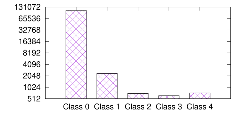
Figure 1. Frequency distribution for each class in the training set using a base 2 log scale

One-vs.-rest. In order to generate a classifier not affected by imbalanced classes we adopt a one-vs.-rest strategy. This is a method that splits a multi-class classification problem into a binary classification problem per class, and maximizing the number of training data per class. Hence, the classifier predicting the quality class $S_{0}$, is fed with $S_{0}$ positive pairs and the same amount of $S_{1},\ldots,S_{4}$ negative pairs (preserving, when possible, a uniform distribution of each negative class). The process is likewise for the other classes. The most notorious impact of this strategy is that each classifier is trained with an optimal number of elements for the positive class. The negative class is chosen so that it maximizes the representativeness of the other classes. Figure 2, depicts the balanced frequency distribution of this strategy. For each $RF_{i}$, observations for class $i$ are considered positive, while all the others are negative.

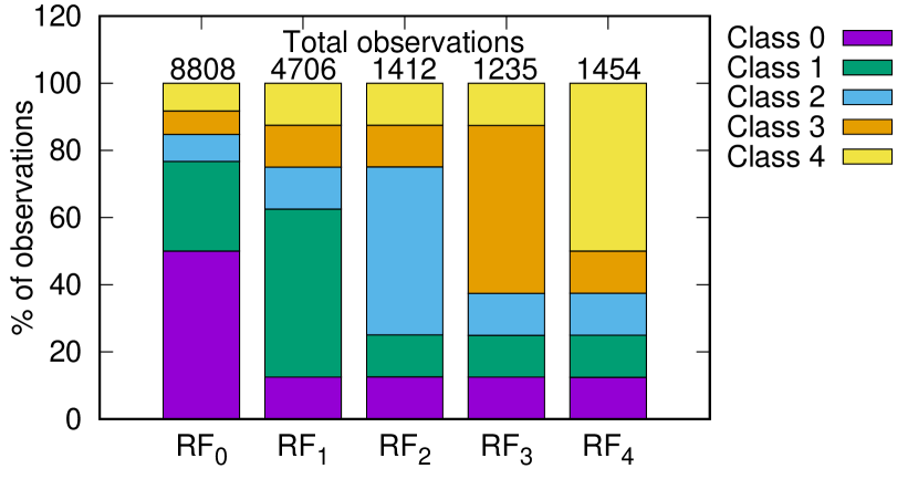
Figure 2. One-vs.-rest frequency distribution per class

Chain classifier. In order to reduce the false positive rate,the different classifiers are connected in a classifier chain architecture. This is a well-studied and effective approach for multi-label classification (Read et al., 2011). Each classifier predicting the probability of class $i$ is trained with the set of distance vectors $D$ and the probabilities of classes $0,\ldots,i-1$. This approach improves the predictive accuracy of the classifier, as we show in Section 5.2. Figure 3 depicts a high-level overview of the architecture used for training. Then, the prediction returned by the classifier is the one with highest probability from each $RF_{i}$.

Figure 3. Chain of 5 random forest classifiers, each $RF_{i}$ is fed with the distances vectors $D$ and the probabilities from the previous classifiers $p_{0},\ldots,p_{i-1}$

Hyperparameter tuning. We perform a model-specific hyperparameter search (Probst et al., 2019). For each $RF_{i}$, we perform a $k$-fold cross-validation training ($k=5$), using an $80\%/20\%$ training/set partition. We, precisely, tune the maxBins, maxDepth and the number of trees. We do not tune other hyperparameters (e.g., feature subset strategy or impurity). We tried the following sets of values: $maxBins=\{35,40,45,50,55,60\}$, $maxDepth=\{20,25,30\}$, and $trees=\{64,$ $70,80,90,100,110,120,$ $128\}$. Table 12, shows the resulting hyperparameter choice and the training time, which was executed on an n1-standard-8 machine hosted by the Google Cloud Platform.

	$\bm{RF_{0}}$	$\bm{RF_{1}}$	$\bm{RF_{2}}$	$\bm{RF_{3}}$	$\bm{RF_{4}}$
MaxBins	55	40	40	60	45
MaxDepth	25	25	30	30	20
Number of trees	120	100	120	80	120
Training time (hrs)	2.92	4.03	4.42	4.98	3.89

Table 12. Selected hyperparameters per model

Ranking. Finally, in order to assign the predicted quality class to a candidate attribute, we initially assign the label with the highest probability from all classifiers. However, some times, the highest probability is close to some of the other class probabilities. Thus, we complement the prediction taking into account the class 0 probability $p_{0}$ (i.e., the probability candidate pair is not joinable) and considering the following two scenarios, where $p_{0}$ will affect the predicted class we finally assign:

1. Assume that $p_{0}>0.5$, however the maximum probability belongs to any $p_{1},\ldots,p_{4}$. Since $p_{0}$ denotes no join predicted, we downgrade the predicted class from $i$ to the class in $0,\ldots,i-1$ with the second highest probability.

2. The second scenario occurs when all $p_{0},\ldots,p_{4}$ have a probability smaller than $0.5$, where we consider that the candidate pair is prone to misclassification. In this situation, if the higher probability belongs to any $p_{1},\ldots,p_{4}$, but it still close to $p_{0}$ (i.e., it does not exceed a threshold), then we downgrade the predicted class from $i$ to the class in $0,\ldots,i-1$ with the second highest probability.

5. Evaluation

In this section, we present the evaluation of our approach. On the one hand, we evaluate the ability of the model to discover quality joins through several experiments as well as its generalizability. On the other hand, we compare its performance with representative state-of-the-art solutions. In order to present transparent experiments and guarantee the reproducibility of results, we created an informative companion website. There, it is possible to find all necessary resources (i.e., source code, datasets, and detailed instructions) needed to reproduce the presented results. The companion website also provides access to $\text{Nextia}_{\text{JD}}$, a tool implementing our approach, as well as a ready-to-use demo in the form of a Jupyter notebook running $\text{Nextia}_{\text{JD}}$.

5.1. Setting

Implementation. We have implemented $\text{Nextia}_{\text{JD}}$ as an extension of Apache Spark 3.0.1. The classification model was trained using its distributed machine learning library MLlib. The runtime methods (i.e., profiling, and generation of rankings ordered by the predicted join quality) are implemented as new operators over the structured data processing library SparkSQL. We leverage on the Catalyst optimizer to efficiently compute the profiles and compare them. As described in the problem statement in Section 3.4, our implementation supports two modes of operation discovery-by-attribute and discovery-by-dataset. The former receives as input a reference Spark dataframe (i.e., a dataset) and one of its attributes, and generates a ranking against a collection of dataframes. The discovery-by-dataset mode does not receive as input a reference attribute, so it runs the discovery process for all attributes from the reference dataframe. Notably, implementing $\text{Nextia}_{\text{JD}}$ on top of Spark brings many other benefits. Firstly, we can benefit from many source connectors and we can easily ingest the most common data formats (e.g., CSV, JSON, XML, Parquet, Avro, etc.). Secondly, our extension benefits from the inherent capacity of Spark to parallelize tasks on top of distributed data.

Test set. For evaluation purposes, we collected 139 independent datasets from those used for the ground truth. We further divided such datasets into 4 testbeds (extra-small, small, medium and large) according to their file size. Table 13 shows the characteristics of each testbed.

Testbed	$\bm{XS}$	$\bm{S}$	$\bm{M}$	$\bm{L}$
File size	$0-1$ MB	$1-100$ MB	$100$ MB $-1$ GB	$>1$ GB
Datasets	28	46	46	19
String attributes	159	590	600	331

Table 13. Characteristics per testbed

Alternatives. We compare our approach with the following state-of-the-art data discovery solutions, whose source code is openly available: LSH Ensemble (Zhu et al., 2016) and FlexMatcher (Chen et al., 2018). No fine tuning was performed in such systems, running the code as provided out-of-the-box. These systems differ in their mode of operation, as described in Section 2, the former being an approach based on comparison by hash, while the latter on comparison by profile. Note we rule out approaches based on comparison by value. Such solutions are not comparable to ours, since their kind of search accuracy is exact and by nature they are not suitable for large-scale scenarios.

Setup. We distinguish two experimental setups. Given that the other systems are not implemented to be executed in a distributed and parallel fashion. In order to perform a fair comparison, the experiments focusing on the quality of the results obtained are run on a quad-core 2018 Macbook Pro 2.30GHz, with a 256GB SSD disk and 16 GB of RAM memory. Then, the experiments that stress the scalability of our method are run on an InfiniBand network 4-node cluster (1 driver, 3 workers), where each machine is equipped with a 1TB SSD disk, 16 CPU 2.27GHz cores and 48GB of RAM memory.

(a)     $XS$ ($0-1$ MB)

0True class $$\begin{matrix}{}&\phantom{00}&\phantom{00}&\phantom{00}&\phantom{00}&\phantom{00}\\ \textbf{4}&\pagecolor{d5}0&\pagecolor{d4}0&\pagecolor{d3}6&\pagecolor{d2}27&\pagecolor{d1}52\\ \textbf{3}&\pagecolor{d4}0&\pagecolor{d3}0&\pagecolor{d2}3&\pagecolor{d1}6&\pagecolor{d2}0\\ \textbf{2}&\pagecolor{d3}2&\pagecolor{d2}0&\pagecolor{d1}45&\pagecolor{d2}4&\pagecolor{d3}0\\ \textbf{1}&\pagecolor{d2}16&\pagecolor{d1}8&\pagecolor{d2}7&\pagecolor{d3}1&\pagecolor{d4}0\\ \textbf{0}&\pagecolor{d1}\raise 0.73193pt\hbox{$\scriptstyle\sim$}&\pagecolor{d2}44&\pagecolor{d3}68&\pagecolor{d4}0&\pagecolor{d5}1\\ {}&\textbf{0}&\textbf{1}&\textbf{2}&\textbf{3}&\textbf{4}\end{matrix}$$ Predicted class

(b)     $S$ ($1-100$ MB)

$$\begin{matrix}&\phantom{00}&\phantom{00}&\phantom{00}&\phantom{00}&\phantom{00}\\ \pagecolor{d5}2&\pagecolor{d4}0&\pagecolor{d3}19&\pagecolor{d2}116&\pagecolor{d1}161\\ \pagecolor{d4}1&\pagecolor{d3}3&\pagecolor{d2}67&\pagecolor{d1}149&\pagecolor{d2}1\\ \pagecolor{d3}44&\pagecolor{d2}1&\pagecolor{d1}93&\pagecolor{d2}10&\pagecolor{d3}0\\ \pagecolor{d2}1553&\pagecolor{d1}390&\pagecolor{d2}197&\pagecolor{d3}0&\pagecolor{d4}0\\ \pagecolor{d1}\raise 0.73193pt\hbox{$\scriptstyle\sim$}&\pagecolor{d2}1718&\pagecolor{d3}394&\pagecolor{d4}6&\pagecolor{d5}0\\ \textbf{0}&\textbf{1}&\textbf{2}&\textbf{3}&\textbf{4}\end{matrix}$$ Predicted class

(c)     $M$ ($100$ MB $-1$ GB)

$$\begin{matrix}\phantom{00}&\phantom{00}&\phantom{00}&\phantom{00}&\phantom{00}\\ \pagecolor{d5}1&\pagecolor{d4}0&\pagecolor{d3}16&\pagecolor{d2}110&\pagecolor{d1}134\\ \pagecolor{d4}4&\pagecolor{d3}3&\pagecolor{d2}41&\pagecolor{d1}169&\pagecolor{d2}0\\ \pagecolor{d3}46&\pagecolor{d2}2&\pagecolor{d1}96&\pagecolor{d2}56&\pagecolor{d3}1\\ \pagecolor{d2}3017&\pagecolor{d1}242&\pagecolor{d2}53&\pagecolor{d3}0&\pagecolor{d4}0\\ \pagecolor{d1}\raise 0.73193pt\hbox{$\scriptstyle\sim$}&\pagecolor{d2}508&\pagecolor{d3}142&\pagecolor{d4}50&\pagecolor{d5}0\\ \textbf{0}&\textbf{1}&\textbf{2}&\textbf{3}&\textbf{4}\end{matrix}$$ Predicted class

(d)     $L$ ($>1$ GB)

$$\begin{matrix}\phantom{00}&\phantom{00}&\phantom{00}&\phantom{00}&\phantom{00}\\ \pagecolor{d5}2&\pagecolor{d4}2&\pagecolor{d3}27&\pagecolor{d2}46&\pagecolor{d1}56\\ \pagecolor{d4}2&\pagecolor{d3}1&\pagecolor{d2}40&\pagecolor{d1}24&\pagecolor{d2}3\\ \pagecolor{d3}0&\pagecolor{d2}14&\pagecolor{d1}78&\pagecolor{d2}28&\pagecolor{d3}0\\ \pagecolor{d2}2317&\pagecolor{d1}97&\pagecolor{d2}92&\pagecolor{d3}0&\pagecolor{d4}0\\ \pagecolor{d1}\raise 0.73193pt\hbox{$\scriptstyle\sim$}&\pagecolor{d2}100&\pagecolor{d3}56&\pagecolor{d4}0&\pagecolor{d5}0\\ \textbf{0}&\textbf{1}&\textbf{2}&\textbf{3}&\textbf{4}\end{matrix}$$ Predicted class

Figure 5. Confusion matrices per file size category. For spacing reasons, values in the bottom left corner are omitted

5.2. Predictive performance

The goal of the first experiment is to assess the classifier’s predictive performance by generating and evaluating the ranking of candidate equi-join predicates for each testbed. We also aim at studying whether the file size impacts the quality of the prediction. With these experiments, we aim at proving the generalizability of our proposal.

Methodology. We will use a confusion matrix to capture the relationship between the true and predicted classes. Additionally, we provide performance metrics for the classifier such as precision, recall and $F_{1}$ score. We first discuss the experiment for all testbeds together, and later do a fine-grained discussion for each testbed.

Results. Figure 4 and Table 14, show, respectively, the confusion matrix and performance metrics for all testbeds. Overall, we evaluated 467965 attributes pairs. We can validate the good performance of the proposed approach by the fact that class 4, denoting the highest quality joins, has the best precision. Our method aims at proposing a ranking according to the predicted join quality, which for the highest value it has almost no false positives. It is also relevant to note that the prediction for class 0, denoting the no join quality, also have both high precision and recall. This is particularly relevant to filter out uninteresting results, and thus reduce the search space when presenting a ranking to the user. We additionally note that, as depicted by the precision and recall measures, predictions corresponding to classes 1 and 2 are highly inaccurate.

0True class $$\begin{matrix}{}&\phantom{000000}&\phantom{000000}&\phantom{000000}&\phantom{000000}&\phantom{000000}\\ \textbf{4}&\pagecolor{d5}5&\pagecolor{d4}2&\pagecolor{d3}68&\pagecolor{d2}299&\pagecolor{d1}393\\ \textbf{3}&\pagecolor{d4}7&\pagecolor{d3}7&\pagecolor{d2}151&\pagecolor{d1}348&\pagecolor{d2}4\\ \textbf{2}&\pagecolor{d3}92&\pagecolor{d2}17&\pagecolor{d1}312&\pagecolor{d2}98&\pagecolor{d3}1\\ \textbf{1}&\pagecolor{d2}6903&\pagecolor{d1}737&\pagecolor{d2}349&\pagecolor{d3}1&\pagecolor{d4}0\\ \textbf{0}&\pagecolor{d1}455084&\pagecolor{d2}2370&\pagecolor{d3}660&\pagecolor{d4}56&\pagecolor{d5}1\\ {}&\textbf{0}&\textbf{1}&\textbf{2}&\textbf{3}&\textbf{4}\end{matrix}$$ Predicted class

Figure 4. Confusion matrix for all testbeds (clearer cells denote a closer proximity w.r.t. the true class)

	Precision	Recall	$\bm{F_{1}}$ score
$(0)\text{ }\texttt{None}$	$0.9848$	$0.9933$	$0.9890$
$(1)\text{ }\texttt{Poor}$	$0.2352$	$0.0922$	$0.1325$
$(2)\text{ }\texttt{Moderate}$	$0.2025$	$0.6000$	$0.3029$
$(3)\text{ }\texttt{Good}$	$0.4339$	$0.6731$	$0.5276$
$(4)\text{ }\texttt{High}$	$0.9849$	$0.5123$	$0.6740$

Table 14. Performance metrics per class for all testbeds

Nevertheless, $\text{Nextia}_{\text{JD}}$ is prepared to be used as an interactive tool. Thus, if we analyze these results from the point of view of a user, most misclassifications are irrelevant. $\text{Nextia}_{\text{JD}}$ shows the results in strict order. First, classes 4 and 3, and then classes 2 and 1 on demand. In this sense, a binary classification meaning likely interesting or likely uninteresting would be a fairer way to evaluate $\text{Nextia}_{\text{JD}}$. When considering these results as a binary problem (interesting: classes 3-4; uninteresting: classes 0-2), the evaluated metrics improve considerably, as shown in Figure 9 and Table 15. Relevantly, we note that $\text{Nextia}_{\text{JD}}$ generates very few false positives; a desirable property for large-scale data discovery problems. We nevertheless highlight the relevance of distinguishing classes 1 and 2 from 0, either for advanced users or because $\text{Nextia}_{\text{JD}}$ could be used for other automatic data discovery problems where such distinction would be relevant. Finally, we analyzed the semantic validity of the join pairs proposed as interesting. Relevantly, 95% of the attribute pairs shown to the user have a semantic relationship.

Next, in Figure 5, we present a fine-grained evaluation of the predictions per file category. Overall, we confirm that regardless of the file size, we accurately predict quality joins. In all cases, we miss between 40% and 50% of class 4 predictions, due to the fact they are downgraded to lower quality classes (mostly to 3). This is the reason for the low recall for that class. However, this is not a concerning aspect, as most candidates will still appear in the ranking but in lower positions. We again highlight the low ratio of false positives generated.

5.3. Comparison with the state-of-the-art

In this experiment we aim at comparing our approach to other data discovery approaches. We perform such evaluation by measuring and comparing their computational complexity and predictive performance.

Methodology. All systems under evaluation, including ours, implement data discovery in two steps. The first step, which we denote pre, builds the core data structures from the datasets. For hash-based methods, such as LSH Ensemble, building the index, while profile-based methods, such as FlexMatcher and ours, create the profiles. Additionally, FlexMatcher will create the predictive models for each new data discovery task. Then, the second step, which we denote as query, consists of computing the prediction leveraging on the previously built data structures. Whenever possible, we decouple both steps and thus read the data structures from disk. This is, however, not the case for LSH Ensemble, as it does not offer any resources to store the index on disk, forcing us to maintain it in memory.

The three systems analyzed have slightly different objectives. In order to perform a fair comparison, we analyze the results from the user perspective. That is, the number of results provided and its degree of interestingness for the user. For that, we use a binary scale, which straightforwardly maps to the output obtained in LSH Ensemble and FlexMatcher. For $\text{Nextia}_{\text{JD}}$, we will reuse the interestingness mapping discussed in the previous experiment: we map classes $\{0,1,2\}$ to the uninteresting class, and classes $\{3,4\}$ to interesting. Applying the same rationale, in LSH Ensemble we consider interesting those pairs with a containment above $50\%$ (i.e., the threshold we considered for our class 3). Finally, FlexMatcher is not parameterizable with a quality threshold and already provides a binary output (i.e., non-joinable/joinable). In this case, non-joinable maps to uninteresting and joinable to interesting.

Results. We evaluated the performance of $\text{Nextia}_{\text{JD}}$, LSH Ensemble and FlexMatcher on each testbed. Both LSH Ensemble and FlexMatcher suffered from scalability issues and were not able to execute testbed $L$. Figure 6, depicts the runtime of the pre phase for each testbed. We can observe that the runtime of all systems is in the same orders of magnitude, however our pre is larger than the rest. This is mainly due to the fact that, to ensure a fair comparison, we did not set Spark on cluster mode. It is well-known that using Spark on centralized mode adds extra overhead of tasks when generating the required data structures, managing partitions, etc. This is not the case for the other systems, which are provided as standalone programs. Nevertheless, $\text{Nextia}_{\text{JD}}$ benefits from Spark robustness and it is the only approach, even in centralized mode, capable of dealing with a large-scale testbed. Furthermore, we note that $\text{Nextia}_{\text{JD}}$ is the only solution able to precompute its pre step (except for binary meta-features).

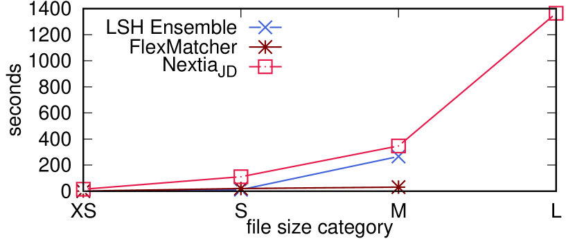
Figure 6. Pre runtime

Regarding the computational performance of the query phase, we distinguish the discovery-by-attribute and discovery-by-dataset scenarios, respectively in Figures 7 and 8. Note that discovery-by-attribute is not available in FlexMatcher. LSH Ensemble excels in both query tasks. This is due to the fact there is no mechanism to persist the index and this task is reduced to an in-memory lookup. FlexMatcher also benefits from fully running in memory but, in this case, the query step suffers from the need to compute some on-the-fly learning models.

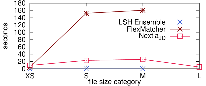
Figure 7. Query runtime (discovery-by-dataset)

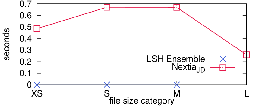
Figure 8. Query runtime (discovery-by-attribute)

As general observation, both approaches are thought to compute their core structures and run in memory, which is the main reason hindering their ability to scale-up. Overall, $\text{Nextia}_{\text{JD}}$ shows a good behaviour in the query step. Importantly, $\text{Nextia}_{\text{JD}}$ is not affected by the dataset cardinality at query time. Indeed, the runtime is directly proportional to the number of attributes, or profiles, to compare.

We now put the focus on comparing the predictive performance of the three approaches. Figure 9 and Table 15, depict, respectively, the confusion matrices and performance metrics using the binary class mapping. Relevantly, the predictive quality of $\text{Nextia}_{\text{JD}}$ and LSH Ensemble are comparable. While LSH Ensemble finds more true positives, it generates much more false positives. As result, $\text{Nextia}_{\text{JD}}$ precision is better. Finally, and aligned with our claim that contemporary profile-based data discovery methods fall short in terms of quality, FlexMatcher generates an extremely large number of false positives reducing its overall quality and making it unfeasible for large-scale scenarios.

(a)     $\text{Nextia}_{\text{JD}}$

..True ..class $$\begin{matrix}{}&\phantom{000000}&\phantom{000000}\\ \textbf{1}&\pagecolor{d4}166&\pagecolor{d1}915\\ \textbf{0}&\pagecolor{d1}419119&\pagecolor{d4}129\\ {}&\textbf{0}&\textbf{1}\end{matrix}$$ Predicted class

(b)     LSH Ensemble

..True ..class $$\begin{matrix}{}&\phantom{000000}&\phantom{000000}\\ \textbf{1}&\pagecolor{d4}55&\pagecolor{d1}1026\\ \textbf{0}&\pagecolor{d1}418338&\pagecolor{d4}910\\ {}&\textbf{0}&\textbf{1}\end{matrix}$$ Predicted class

(c)     FlexMatcher

..True ..class $$\begin{matrix}{}&\phantom{000000}&\phantom{000000}\\ \textbf{1}&\pagecolor{d4}572&\pagecolor{d1}509\\ \textbf{0}&\pagecolor{d1}381493&\pagecolor{d4}37755\\ {}&\textbf{0}&\textbf{1}\end{matrix}$$ Predicted class

Figure 9. Combined confusion matrices for each system on testbeds $XS,S,M$

	Precision	Recall	$\bm{F_{1}}$ score
$\text{Nextia}_{\text{JD}}$	$0.8764$	$0.8464$	$0.8611$
LSH Ensemble	$0.5299$	$0.9491$	$0.6800$
FlexMatcher	$0.0133$	$0.4708$	$0.0258$

Table 15. Performance metrics using binary classes for each system under evaluation on testbeds $XS,S,M$

Then, Figure 10 drills deeper  into  the  comparison  between   $\text{Nextia}_{\text{JD}}$  and LSH Ensemble. We assigned a quality class to LSH Ensemble by running it several times and using a different containment threshold each time, as defined in our quality classes (i.e., 0.75, 0.5, 0.25 and 0.1). There, we observe relevant differences on the predictions computed. In general, our approach is more conservative, in the sense that we produce less false positives at expenses of sacrificing some true positives. Overall, this improves the precision of our approach by reducing the number of false positives shown to the user. As general observation, both approaches follow slightly different objectives and $\text{Nextia}_{\text{JD}}$ is more suitable for large-scale scenarios, both for its scale-up capacity and high precision, which guarantees the user will not be overwhelmed with large rankings including false positives.

(a)     $\text{Nextia}_{\text{JD}}$ ($XS,S,M$)

0True class $$\begin{matrix}{}&\phantom{000000}&\phantom{000000}&\phantom{000000}&\phantom{000000}&\phantom{000000}\\ \textbf{4}&\pagecolor{d5}3&\pagecolor{d4}0&\pagecolor{d3}41&\pagecolor{d2}253&\pagecolor{d1}337\\ \textbf{3}&\pagecolor{d4}5&\pagecolor{d3}6&\pagecolor{d2}111&\pagecolor{d1}324&\pagecolor{d2}1\\ \textbf{2}&\pagecolor{d3}92&\pagecolor{d2}3&\pagecolor{d1}234&\pagecolor{d2}70&\pagecolor{d3}1\\ \textbf{1}&\pagecolor{d2}4586&\pagecolor{d1}640&\pagecolor{d2}257&\pagecolor{d3}1&\pagecolor{d4}0\\ \textbf{0}&\pagecolor{d1}410433&\pagecolor{d2}2270&\pagecolor{d3}604&\pagecolor{d4}56&\pagecolor{d5}1\\ {}&\textbf{0}&\textbf{1}&\textbf{2}&\textbf{3}&\textbf{4}\end{matrix}$$ Predicted class

(b)     LSH Ensemble ($XS,S,M$)

0True class $$\begin{matrix}{}&\phantom{000000}&\phantom{000000}&\phantom{000000}&\phantom{000000}&\phantom{000000}\\ \textbf{4}&\pagecolor{d5}1&\pagecolor{d4}0&\pagecolor{d3}0&\pagecolor{d2}5&\pagecolor{d1}628\\ \textbf{3}&\pagecolor{d4}0&\pagecolor{d3}0&\pagecolor{d2}54&\pagecolor{d1}84&\pagecolor{d2}309\\ \textbf{2}&\pagecolor{d3}17&\pagecolor{d2}27&\pagecolor{d1}180&\pagecolor{d2}111&\pagecolor{d3}65\\ \textbf{1}&\pagecolor{d2}4606&\pagecolor{d1}191&\pagecolor{d2}185&\pagecolor{d3}497&\pagecolor{d4}5\\ \textbf{0}&\pagecolor{d1}412425&\pagecolor{d2}447&\pagecolor{d3}260&\pagecolor{d4}227&\pagecolor{d5}5\\ {}&\textbf{0}&\textbf{1}&\textbf{2}&\textbf{3}&\textbf{4}\end{matrix}$$ Predicted class

Figure 10. Confusion matrices using 5 quality classes for $\text{Nextia}_{\text{JD}}$ and LSH Ensemble

5.4. Scalability

Since we target large-scale scenarios, we evaluate the scalability of our $\text{Nextia}_{\text{JD}}$ in such settings. We experiment with different file sizes both in terms of rows and columns.

Methodology. As shown in Figure 6, our most intensive task with regard to computational resources is the generation of attribute profiles from datasets. We hence performed a stress test of this component by means of two experiments. First, we generated a 10GB base CSV file with 5 columns and systematically extended it in batches of 10GBs, up to 60GBs. Next, we followed a similar strategy with regard to columns. We created a 20GB base file that was systematically extended with a new duplicate column each time. The resulting files were stored in a Hadoop HDFS cluster, using the default block size and replication parameters. In order to simulate a realistic large-scale scenario, we also converted each input file to Apache Parquet format. Parquet is an specialized hybrid layout that fragments data into row group partitions (i.e., physically-independent columns), while it also embeds numerous statistics to optimize queries. To evaluate the scalability of our approach in terms of distribution, we compute the profiling runtime using $n$ Spark workers (cf. HDFS datanodes) in the range $1\ldots 3$.

Results. Figure 11 depicts the profiling runtime for an increasing file size. Regardless of the number of workers and data format used, the runtime linearly scales with the file size. As expected, profiling Parquet files are much more efficient than CSV ones (i.e., an approximate 4x to 5x speed-up), as we can benefit from statistics and compression when computing certain meta-features.

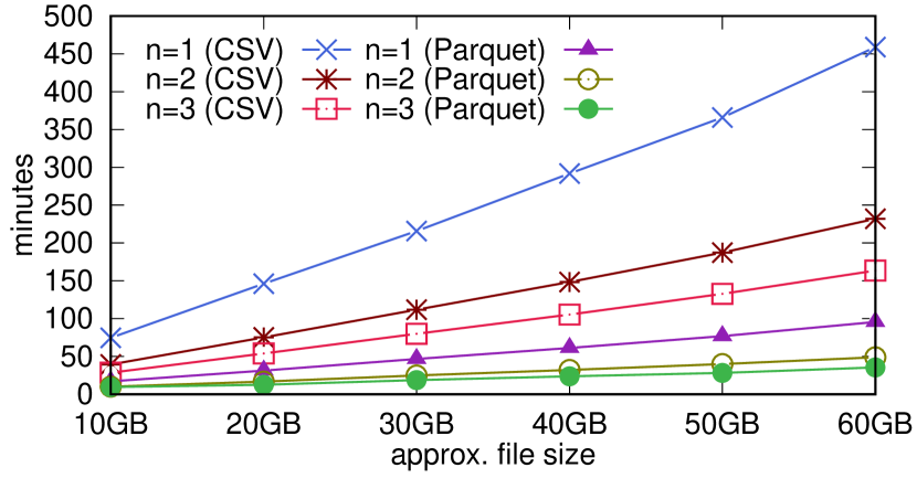
Figure 11. Profiling runtime over an increasing file size

As depicted in Figure 12, we can also observe that the profiling runtime trend scales linearly with the number of columns. Similarly to the previous case, using Parquet significantly speeds up the process, here with a 7x to 8x factor.

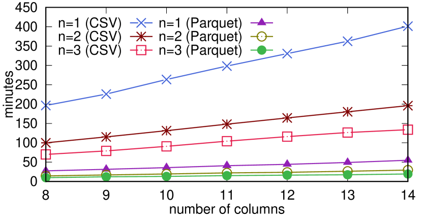
Figure 12. Profiling runtime over an increasing number of columns

Finally, in Table 16, we show the average profile size per each testbed. The disk usage is proportional to both the number of rows and columns. Although the number of columns is the leading factor for the profiling size, the dataset cardinality impacts on the size of some meta-features (e.g., frequent words, soundex, etc.). In any case, the profile sizes are reasonable. Thus, they can be precomputed offline and stored together with the dataset as metadata. The only exception to this would be binary meta-features. As final conclusion, these experiments show that our approach does not introduce any blocking factor hindering parallelism and can fully benefit from it.

Testbed	Average profile size (KBs)
$XS$	$132$
$S$	$343$
$M$	$282$
$L$	$398.1$

Table 16. Average profile size per testbed

5.5. Discovery of semantic non-syntactic relationships

This last experiment aims at scrutinizing the behaviour of our model in front of semantic non-syntactic joinable pairs (see Section 3).

Methodology. We manually curated a test dataset $D$ of 532 semantic non-syntactic attribute pairs. In order to devise their true label, we applied the following three transformations: (1) string cleaning (e.g., remove accents, dashes, etc.), (2) dictionary lookup (e.g., country codes to country names, author names to full names, etc.), and (3) unwind collections. Accordingly, we were able to generate an approximate ground truth $D^{\prime}$ applying the quality definition over the transformed dataset. Using that, we were able to evaluate the performance of $\text{Nextia}_{\text{JD}}$ on $D$ by comparing the predictions to the true labels in $D^{\prime}$.

Results. At first, $\text{Nextia}_{\text{JD}}$ yielded low predictive performance. A detailed analysis revealed that (i) a strict quality definition and (ii) the chain classifier strategy were drastically penalizing this kind of join relationship. These factors were identified as the main reasons for our high precision and low number of false positives. As consequence, we trained a new set of classifiers (using the same ground truth as shown in Section 4.3), deactivating the chain classifier strategy and keeping the same join quality definition. Figure 13 depicts the results in a confusion matrix. This new model classified 48.87% of the true positives as classes 1-3. Nonetheless, most of these pairs are misclassified to lower quality classes than their true class. Note that non surprisingly, no pair was predicted as quality 4, due to our strict definition of high quality joins, hard to achieve for semantic non-syntactic attributes. A closer look to the predicted pairs showed the complexity of identifying such kind of pairs with our quality join definition and current set of meta-features. Although these results show that our method only works for semantic and/or syntactic relationships, we do believe they are promising.As a matter of fact, the meta-features used in our classifiers (see Table 11) limit the ability to detect semantic non-syntactic pairs. Specifically, Syntactic meta-features are mostly writing off such pairs. Yet, we were able to identify some due to the role played by the Cardinalties and Value distribution meta-features. We conclude that a new model should be devised, with specific meta-features to capture the special nature of these relationships.

0True class $$\begin{matrix}{}&\phantom{000000}&\phantom{000000}&\phantom{000000}&\phantom{000000}&\phantom{000000}\\ \textbf{4}&\pagecolor{d5}90&\pagecolor{d4}46&\pagecolor{d3}47&\pagecolor{d2}22&\pagecolor{d1}0\\ \textbf{3}&\pagecolor{d4}36&\pagecolor{d3}24&\pagecolor{d2}32&\pagecolor{d1}7&\pagecolor{d2}0\\ \textbf{2}&\pagecolor{d3}37&\pagecolor{d2}15&\pagecolor{d1}20&\pagecolor{d2}0&\pagecolor{d3}0\\ \textbf{1}&\pagecolor{d2}68&\pagecolor{d1}23&\pagecolor{d2}3&\pagecolor{d3}1&\pagecolor{d4}0\\ \textbf{0}&\pagecolor{d1}41&\pagecolor{d2}19&\pagecolor{d3}1&\pagecolor{d4}0&\pagecolor{d5}0\\ {}&\textbf{0}&\textbf{1}&\textbf{2}&\textbf{3}&\textbf{4}\end{matrix}$$ Predicted class

Figure 13. Semantic non-syntactic attributes identified

6. Conclusions and future work

We have presented a novel learning-based approach for data discovery on large-scale repositories of heterogeneous, independently created datasets. Our work is motivated by (i) the poor predictive performance of current profile-based solutions, and (ii) the inability to scale-up of hash-based approaches, as well as their low precision, which is undesirable for large-scale scenarios. In order to overcome these limitations, we propose a scalable method yielding good precision, and grounded on a novel qualitative definition of join quality. Further, we implemented our approach in a tool called $\text{Nextia}_{\text{JD}}$. We have experimentally shown that despite being a profile-based approach, $\text{Nextia}_{\text{JD}}$ presents a similar predictive performance to that of hash-based solutions, yet better adapted for large-scale scenarios, while benefiting from linear scalability.

As future work, we look for adapting our approach to detect semantic non-syntactic join relationships (i.e., requiring some simple transformation on the values before joining). Based on such predictions, the system should be able to propose the required transformations to join.

References

- (1)
- Abadi et al. (2019) Daniel Abadi, Anastasia Ailamaki, David Andersen, Peter Bailis, Magdalena Balazinska, Philip A. Bernstein, Peter A. Boncz, Surajit Chaudhuri, Alvin Cheung, AnHai Doan, Luna Dong, Michael J. Franklin, Juliana Freire, Alon Y. Halevy, Joseph M. Hellerstein, Stratos Idreos, Donald Kossmann, Tim Kraska, Sailesh Krishnamurthy, Volker Markl, Sergey Melnik, Tova Milo, C. Mohan, Thomas Neumann, Beng Chin Ooi, Fatma Ozcan, Jignesh Patel, Andrew Pavlo, Raluca A. Popa, Raghu Ramakrishnan, Christopher Ré, Michael Stonebraker, and Dan Suciu. 2019. The Seattle Report on Database Research. SIGMOD Rec. 48, 4 (2019), 44–53.
- Abedjan et al. (2015) Ziawasch Abedjan, Lukasz Golab, and Felix Naumann. 2015. Profiling relational data: a survey. VLDB J. 24, 4 (2015), 557–581.
- Abiteboul et al. (1995) Serge Abiteboul, Richard Hull, and Victor Vianu. 1995. Foundations of Databases. Addison-Wesley.
- Balazinska et al. (2020) Magda Balazinska, Surajit Chaudhuri, Anastasia Ailamaki, Juliana Freire, Sailesh Krishnamurthy, and Michael Stonebraker. 2020. The Next 5 Years: What Opportunities Should the Database Community Seize to Maximize its Impact?. In SIGMOD Conference. ACM, 411–414.
- Bogatu et al. (2020) Alex Bogatu, Alvaro A. A. Fernandes, Norman W. Paton, and Nikolaos Konstantinou. 2020. Dataset Discovery in Data Lakes. In ICDE. IEEE, 709–720.
- Breiman (2001) Leo Breiman. 2001. Random Forests. Mach. Learn. 45, 1 (2001), 5–32.
- Broder (1997) Andrei Z. Broder. 1997. On the resemblance and containment of documents. In SEQUENCES. IEEE, 21–29.
- Chen et al. (2018) Chen Chen, Behzad Golshan, Alon Y. Halevy, Wang-Chiew Tan, and AnHai Doan. 2018. BigGorilla: An Open-Source Ecosystem for Data Preparation and Integration. IEEE Data Eng. Bull. 41, 2 (2018), 10–22.
- Deng et al. (2017) Dong Deng, Albert Kim, Samuel Madden, and Michael Stonebraker. 2017. SilkMoth: An Efficient Method for Finding Related Sets with Maximum Matching Constraints. Proc. VLDB Endow. 10, 10 (2017), 1082–1093.
- Doan et al. (2003) AnHai Doan, Pedro M. Domingos, and Alon Y. Halevy. 2003. Learning to Match the Schemas of Data Sources: A Multistrategy Approach. Mach. Learn. 50, 3 (2003), 279–301.
- Fernandez et al. (2018) Raul Castro Fernandez, Essam Mansour, Abdulhakim Ali Qahtan, Ahmed K. Elmagarmid, Ihab F. Ilyas, Samuel Madden, Mourad Ouzzani, Michael Stonebraker, and Nan Tang. 2018. Seeping Semantics: Linking Datasets Using Word Embeddings for Data Discovery. In ICDE. IEEE Computer Society, 989–1000.
- Fernandez et al. (2019) Raul Castro Fernandez, Jisoo Min, Demitri Nava, and Samuel Madden. 2019. Lazo: A Cardinality-Based Method for Coupled Estimation of Jaccard Similarity and Containment. In ICDE. IEEE, 1190–1201.
- Golshan et al. (2017) Behzad Golshan, Alon Y. Halevy, George A. Mihaila, and Wang-Chiew Tan. 2017. Data Integration: After the Teenage Years. In PODS. ACM, 101–106.
- Jiménez-Ruiz and Grau (2011) Ernesto Jiménez-Ruiz and Bernardo Cuenca Grau. 2011. LogMap: Logic-Based and Scalable Ontology Matching. In International Semantic Web Conference (1) (Lecture Notes in Computer Science), Vol. 7031. Springer, 273–288.
- Kejriwal and Miranker (2015) Mayank Kejriwal and Daniel P. Miranker. 2015. Semi-supervised Instance Matching Using Boosted Classifiers. In ESWC (Lecture Notes in Computer Science), Vol. 9088. Springer, 388–402.
- Levenshtein (1966) Vladimir Levenshtein. 1966. Binary Codes Capable of Correcting Deletions, Insertions and Reversals. Soviet Physics Doklady 10 (1966), 707.
- Miller et al. (2018) Renée J. Miller, Fatemeh Nargesian, Erkang Zhu, Christina Christodoulakis, Ken Q. Pu, and Periklis Andritsos. 2018. Making Open Data Transparent: Data Discovery on Open Data. IEEE Data Eng. Bull. 41, 2 (2018), 59–70.
- Nargesian et al. (2020) Fatemeh Nargesian, Ken Q. Pu, Erkang Zhu, Bahar Ghadiri Bashardoost, and Renée J. Miller. 2020. Organizing Data Lakes for Navigation. In SIGMOD Conference. ACM, 1939–1950.
- Nargesian et al. (2019) Fatemeh Nargesian, Erkang Zhu, Renée J. Miller, Ken Q. Pu, and Patricia C. Arocena. 2019. Data Lake Management: Challenges and Opportunities. Proc. VLDB Endow. 12, 12 (2019), 1986–1989.
- Panda et al. (2009) Biswanath Panda, Joshua Herbach, Sugato Basu, and Roberto J. Bayardo. 2009. PLANET: Massively Parallel Learning of Tree Ensembles with MapReduce. Proc. VLDB Endow. 2, 2 (2009), 1426–1437.
- Probst et al. (2019) Philipp Probst, Marvin N. Wright, and Anne-Laure Boulesteix. 2019. Hyperparameters and tuning strategies for random forest. Wiley Interdiscip. Rev. Data Min. Knowl. Discov. 9, 3 (2019).
- Read et al. (2011) Jesse Read, Bernhard Pfahringer, Geoff Holmes, and Eibe Frank. 2011. Classifier chains for multi-label classification. Mach. Learn. 85, 3 (2011), 333–359.
- Stonebraker and Ilyas (2018) Michael Stonebraker and Ihab F. Ilyas. 2018. Data Integration: The Current Status and the Way Forward. IEEE Data Eng. Bull. 41, 2 (2018), 3–9.
- Xiao et al. (2011) Chuan Xiao, Wei Wang, Xuemin Lin, Jeffrey Xu Yu, and Guoren Wang. 2011. Efficient similarity joins for near-duplicate detection. ACM Trans. Database Syst. 36, 3 (2011), 15:1–15:41.
- Yang et al. (2019) Yang Yang, Ying Zhang, Wenjie Zhang, and Zengfeng Huang. 2019. GB-KMV: An Augmented KMV Sketch for Approximate Containment Similarity Search. In ICDE. IEEE, 458–469.
- Zhu et al. (2019) Erkang Zhu, Dong Deng, Fatemeh Nargesian, and Renée J. Miller. 2019. JOSIE: Overlap Set Similarity Search for Finding Joinable Tables in Data Lakes. In SIGMOD Conference. ACM, 847–864.
- Zhu et al. (2016) Erkang Zhu, Fatemeh Nargesian, Ken Q. Pu, and Renée J. Miller. 2016. LSH Ensemble: Internet-Scale Domain Search. Proc. VLDB Endow. 9, 12 (2016), 1185–1196.