Multi-ring, stripe, and super-lattice solitons in a spin-orbit coupled spin-1 condensate

Abstract

We demonstrate exotic stable quasi-two-dimensional solitons in a Rashba or a Dresselhaus spin-orbit (SO) coupled hyperfine spin-1 ($F=1$) trap-less antiferromagnetic Bose-Einstein condensate using the mean-field Gross-Pitaevskii equation. For weak SO coupling, the solitons are of the $(-1,0,+1)$ or $(+1,0,-1)$ type with intrinsic vorticity, for Rashba or Dresselhaus SO coupling, where the numbers in the parentheses denote angular momentum in spin components $F_{z}=+1,0,-1$, respectively. For intermediate SO coupling, the solitons have multi-ring structure maintaining the above-mentioned vortices in respective components. For larger SO coupling, super-lattice solitons with a square-lattice structure in total density are found in addition to stripe solitons with stripe pattern in component densities with no periodic modulation in total density.

A bright soliton or a soliton is a one-dimensional (1D) shape-preserving solitary wave stabilized by a cancellation of dispersive forces and nonlinear attraction r1 . Quasi-1D solitons have been observed in a Bose-Einstein condensate (BEC) of ⁷Li r2 and ⁸⁵Rb r3 atoms following a theoretical suggestion r5 . However, solitons cannot be stabilized in two (2D) townes and three dimensions (3D) r1 .

The interest in the creation of spin-orbit (SO) coupling in a BEC increased after the observation of a hyperfine spin-1 spinor BEC of ²³Na atoms exptspinor . Although there cannot be a natural SO coupling in a neutral atom, it is possible to introduce an artificial synthetic SO coupling by tuned Raman lasers coupling the different spin states thso ; exptsob . Two such possible SO couplings are due to Dresselhaus SOdre and Rashba SOras . An equal mixture of Dresselhaus and Rashba SO couplings has been experimentally realized in a pseudo spin-1/2 ⁸⁷Rb exptso and ²³Na na-solid BEC of $F_{z}=0,-1$ spin states. Later, an SO-coupled spin-1 ⁸⁷Rb BEC of $F_{z}=\pm 1,0$ states was observed exptsp1 .

A pseudo spin-1/2 SO-coupled BEC can sustain a quasi-1D quasi-1d or a quasi-2D quasi-2d or a 3D quasi-3d soliton. In a spin-1/2 SO-coupled BEC, quantum half-vortex solitons half-vortex have also been studied and multi-ring and rotating solitons were also found in a periodic potential radper . Stability of these solitons have also been studied recently stab . A spin-1 SO-coupled BEC also sustains a quasi-1D quasi-1d1 or a quasi-2D quasi-2d1 or a 3D quasi-3d1 soliton.

Here we undertake a comprehensive study of solitons in a spin-1 quasi-2D Rashba or a Dresselhaus SO-coupled antiferromagnetic BEC. For a weakly Rashba or Dresselhaus SO-coupled spin-1 BEC (SO-coupling strength $\gamma\lessapprox 0.75$), the soliton is of the $(\mp 1,0,\pm 1)$ type of angular momenta $\mp 1,0,\pm 1$ in components $F_{z}=+1,0,-1$ kita ; quasi-2d1 , where the positive (negative) sign denotes a vortex (an antivortex) and the upper (lower) sign corresponds to Rashba (Dresselhaus) SO coupling. For medium SO-coupling, we find $(\mp 1,0,\pm 1)$-type multi-ring solitons for Rashba or Dresselhaus SO couplings, maintaining the above-mentioned vortices at the center of respective components. For larger SO-coupling, two types of quasi-degenerate solitons are found. The first type has maxima and minima in density forming a stripe pattern. In the second type, matter is spontaneously distributed on a 2D square lattice. For a Dresselhaus SO-coupled BEC, the density and energy of the solitons are the same as in the case of Rashba coupling, but the two wave functions are different.

The pursuit of a super-solid sprsld is a fascinating subject in different areas of condensed matter physics. A super-solid is a quantum state where matter forms a spatially-ordered rigid structure, breaking continuous translational symmetry, as in a crystalline solid, and also enjoys friction-less flow as in a super-fluid, breaking Gauge symmetry. Although, super-solidity was never confirmed in super-fluid helium solhel , more recently, it has been suggested losh and observed dipolar in a dipolar BEC. In a spin-1/2 SO-coupled BEC, super-solidity has been realized experimentally exp-stripe in the form of a quasi-1D stripe pattern in density stripe ; stripe2 ; sinha . The present solitons with a 2D square-lattice structure in total density 2020 , viz. Figs. 5(c) and (f) and Fig. 4(f), sharing properties with a conventional supersolid, will be termed super-lattice solitons in the following as suggested in Refs. stripe ; 2020 . The super-lattice solitons are expected to possess coexisting order parameters with super-solid-like properties leading to a periodic spatial structure in total density stripe ; 2020 , as illustrated in Fig. 1 of Ref. 2020 , in Fig. 1 of Ref. stripe ; sting and in Fig. 1(e) of Ref. sinha ; sinha2 . The multi-ring, viz. Fig. 3, and stripe, viz. Figs. 4(a)-(c), solitons only exhibit a periodic structure in the component densities, due to a phase separation among the components without any periodic structure in the total density. A super-lattice soliton is a unique example of spontaneous 2D crystallization in a free condensed matter system and a study of this may enhance the knowledge about the origin of crystal formation in solids under controlled conditions.

We consider a BEC of $N$ atoms, each of mass $m$, under a harmonic trap $V({\bf r})={m}\omega_{z}^{2}z^{2}/2$ of frequency $\omega_{z}$ in the $z$ direction and free in the $x-y$ plane. After integrating out the $z$ coordinate quasi12d , the single particle Hamiltonian of the SO-coupled BEC is exptso

$$H_{0}=-\frac{\hbar^{2}}{2m}\nabla_{\boldsymbol{\rho}}^{2}+\gamma[\eta p_{y}\Sigma_{x}-p_{x}\Sigma_{y}],$$ (1)

where ${\boldsymbol{\rho}}\equiv\{x,y\}$, $\nabla_{\boldsymbol{\rho}}^{2}=(\partial^{2}/\partial x^{2}+\partial^{2}/\partial y^{2})\equiv(\partial_{x}^{2}+\partial_{y}^{2})$, $\gamma$ is the strength of the SO-coupling term in square bracket, where $\eta=+1$ for Rashba coupling, $\eta=-1$ for Dresselhaus coupling, and $\eta=0$ for an equal mixture of Rashba and Dresselhaus couplings, $p_{x}=-i\hbar\partial_{x},p_{y}=-i\hbar\partial_{y}$ and the spin matrices $\Sigma_{x}$ and $\Sigma_{y}$ are

$$\Sigma_{x}=\frac{1}{\sqrt{2}}\begin{pmatrix}0&1&0\\ 1&0&1\\ 0&1&0\end{pmatrix},\quad\Sigma_{y}=\frac{i}{\sqrt{2}}\begin{pmatrix}0&-1&0\\ 1&0&-1\\ 0&1&0\end{pmatrix}.$$ (2)

A quasi-2D Rashba SO-coupled spin-1 spinor BEC is described by the following set of Gross-Pitaevskii equations r6 at zero temperature for spin components $F_{z}=\pm 1,0$ thspinor ; thspinorb

$$i\partial_{t} \psi_{\pm 1}({\boldsymbol{\rho}})=\left[{\cal H}+{c_{2}}\left(n_{\pm 1}-n_{\mp 1}+n_{0}\right)\right]\psi_{\pm 1}({\boldsymbol{\rho}})$$

$$+ \left\{c_{2}\psi_{0}^{2}({\boldsymbol{\rho}})\psi_{\mp 1}^{*}({\boldsymbol{\rho}})\right\}-i{\widetilde{\gamma}}(\eta\partial_{y}\pm i\partial_{x})\psi_{0}({\boldsymbol{\rho}})\,,$$ (3)

$$i\partial_{t} \psi_{0}({\boldsymbol{\rho}})=\left[{\cal H}+{c_{2}}\left(n_{+1}+n_{-1}\right)\right]\psi_{0}({\boldsymbol{\rho}})+\big{\{}2c_{2}\psi_{+1}({\boldsymbol{\rho}})$$

$$\times \psi_{-1}({\boldsymbol{\rho}})\psi_{0}^{*}({\boldsymbol{\rho}})\big{\}}{-i{\widetilde{\gamma}}[-i\partial_{x}\phi_{-1}({\boldsymbol{\rho}})+\eta\partial_{y}\phi_{+1}({\boldsymbol{\rho}})]}\,,$$ (4)

$${\cal H}= -\frac{1}{2}\nabla^{2}_{\boldsymbol{\rho}}+c_{0}n,$$ (5)

$$c_{0}= \frac{2{N}\sqrt{2\pi}(a_{0}+2a_{2})}{3},\quad c_{2}=\frac{2{N}\sqrt{2\pi}(a_{2}-a_{0})}{3},$$ (6)

where $\phi_{\pm 1}({\boldsymbol{\rho}})=\psi_{+1}({\boldsymbol{\rho}})\pm\psi_{-1}({\boldsymbol{\rho}})$, $\partial_{t}\equiv\partial/\partial t$, $\widetilde{\gamma}=\gamma/\sqrt{2}$, $n_{j}=|\psi_{j}|^{2},j=\pm 1,0$ are the densities of spin components $F_{z}=\pm 1,0$, and $n({\boldsymbol{\rho}})=\sum_{j}n_{j}({\boldsymbol{\rho}})$ the total density, $a_{0}$ and $a_{2}$ are the scattering lengths in the total spin 0 and 2 channels, respectively, and the asterisk denotes complex conjugate. All quantities in Eqs. (Multi-ring, stripe, and super-lattice solitons in a spin-orbit coupled spin-1 condensate)-(6) and in the following are dimensionless; this is achieved by expressing length ($a_{0},a_{2},x,y,z$) in units of oscillator length $l_{0}\equiv\sqrt{\hbar/{m}\omega_{z}}$, density in units of $l_{0}^{-2}$, energy in units of $\hbar\omega_{z}$, and time in units of $\omega_{z}^{-1}$. A spin-1 spinor BEC is classified into two magnetic phases thspinor : ferromagnetic ($c_{2}<0$) and antiferromagnetic ($c_{2}>0$). The normalization condition is ${\textstyle\int}n({\boldsymbol{\rho}})\,d{\boldsymbol{\rho}}=1\,.$ The time-independent version of Eqs. (Multi-ring, stripe, and super-lattice solitons in a spin-orbit coupled spin-1 condensate)-(Multi-ring, stripe, and super-lattice solitons in a spin-orbit coupled spin-1 condensate), appropriate for stationary solutions, can be derived from the energy functional

$$E[\psi] =\frac{1}{2}\int d{\boldsymbol{\rho}}\Big{\{}\sum_{j}|\nabla_{\boldsymbol{\rho}}\psi_{j}|^{2}{-2\mu n}+c_{0}n^{2}+c_{2}\big{[}n_{+1}^{2}$$

$$+n_{-1}^{2}+2(n_{+1}n_{0}+n_{-1}n_{0}-n_{+1}n_{-1}+\psi_{-1}^{*}\psi_{0}^{2}\psi_{+1}^{*}$$

$$+\psi_{-1}\psi_{0}^{*2}\psi_{+1})\big{]}-2i\widetilde{\gamma}\big{[}\eta\psi_{0}^{*}\partial_{y}\phi_{+1}+\eta\phi_{+1}^{*}\partial_{y}\psi_{0}$$

$$-i\psi_{0}^{*}\partial_{x}\phi_{-1}+i\phi_{-1}^{*}\partial_{x}\psi_{0}\big{]}\Big{\}}{+\mu},$$ (7)

where $\mu$ is the chemical potential.

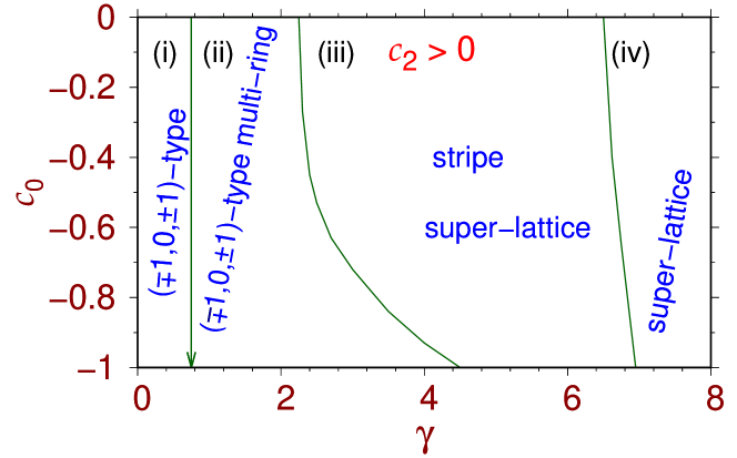
Figure 1: The $c_{0}$ versus $\gamma$ phase plot showing soliton formation in a Rashba or a Dresselhaus SO-coupled spin-1 antiferromagnetic BEC in different regions of parameter space: formation of (i) ($\mp 1,0,\pm 1$)-type, (ii) ($\mp 1,0,\pm 1$)-type multi-ring, (iii) stripe, and (iii,iv) super-lattice solitons. The upper (lower) sign correspond to Rashba (Dresselhaus) coupling. Results in all figures are plotted in dimensionless units.

To solve Eqs. (Multi-ring, stripe, and super-lattice solitons in a spin-orbit coupled spin-1 condensate) and (Multi-ring, stripe, and super-lattice solitons in a spin-orbit coupled spin-1 condensate) numerically, we propagate these in time by the split-time-step Crank-Nicolson discretization scheme bec2009 with the boundary condition that the wave-funcion components and their first derivatives vanish at the boundary while using a space step of 0.1 and a time step of 0.001 for imaginary-time propagation and 0.00025 for real-time propagation. All calculations of soliton profiles employ imaginary-time approach with the conservation of normalization during time propagation, which finds the lowest-energy solution of each type. Real-time propagation is used to test the stability of the solitons. Magnetization ($=\int d{\boldsymbol{\rho}[n_{+1}-n_{-1}]}$) is not a good quantum number and is left to freely evolve during time propagation to attain a final converged value consistent with the parameters of the problem. However, this converged value was found to be zero in all cases studied.

We study the formation of a quasi-2D soliton in a self-attractive $(c_{0}<0)$ spin-1 antiferromagnetic BEC for different sets of parameters: the nonlinearities $c_{0},c_{2}$ and SO-coupling strength $\gamma$. The scenario of soliton formation for Rashba or Dresselhaus SO coupling is illustrated in the phase plot of $c_{0}$ versus $\gamma$ for $c_{2}>0$ in Fig. 1. Solitons of type $(\mp 1,0,\pm 1)$ are formed in region (i), whereas $(\mp 1,0,\pm 1)$-type multi-ring solitons are formed in region (ii). In region (iii), stripe solitons are formed and super-lattice solitons are possible in regions (iii) and (iv). The phase plot remains unchanged independent of the value of $c_{2}$ unless it is too large. No visible change in the phase plot is found for $10>c_{2}>0$, consistent with an analytical result that the density and energy of a weakly SO-coupled spin-1 BEC soliton are independent of $c_{2}$ for quasi-1D quasi-1d12 and quasi-2D quasi-2d1 settings. For smaller values of $c_{0}$ ($c_{0}<-1$), because of an excess of attraction the soliton acquires a small size of the order of the lattice period and the crystalline structure is lost.

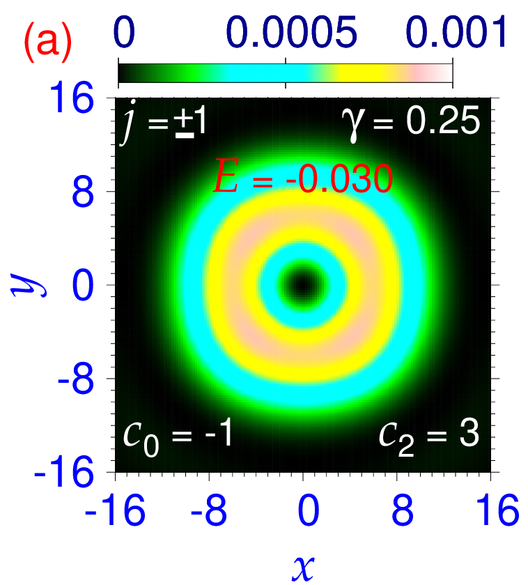
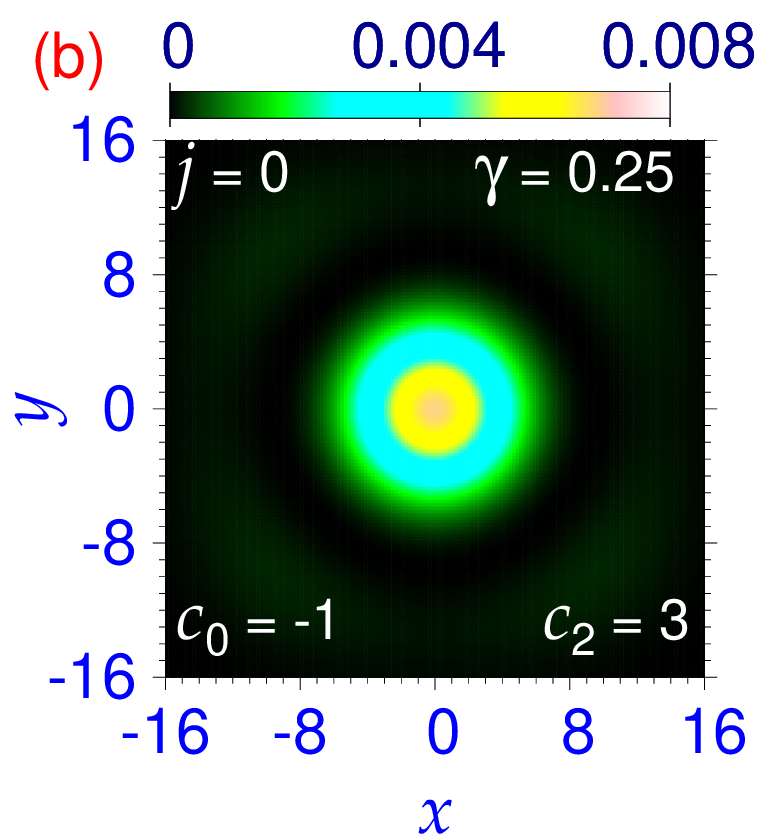
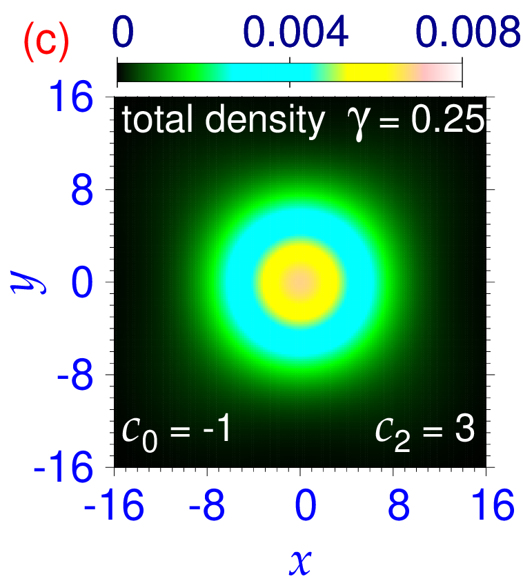
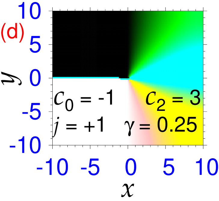
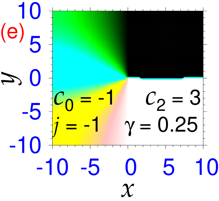
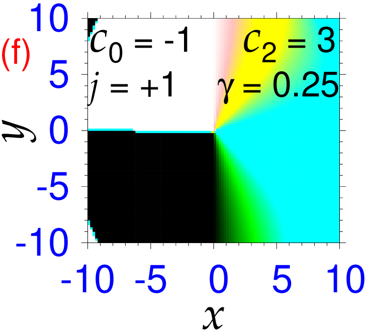
Figure 2: Contour plot of density $n_{j}$ of a $(\mp 1,0,\pm 1)$-type spin-1 Rashba or Dresselhaus SO-coupled BEC soliton for components (a) $j=\pm 1$, (b) $j=0$ and (c) total density. The phases of the wave functions of components $j=\pm 1$ of the $(-1,0,+1)$-type Rashba SO-coupled soliton shown in (a) are displayed in (d) and (e). The same of components $j=\pm 1$ for a $(+1,0,-1)$-type spin-1 Dresselhaus SO-coupled BEC soliton are illustrated in (f) and (g).

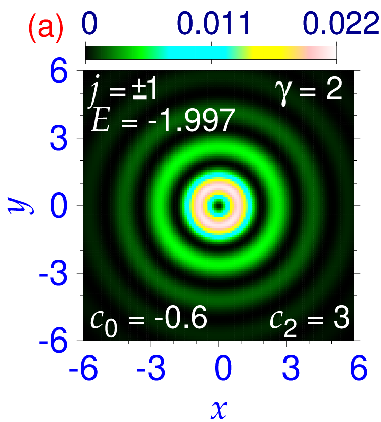
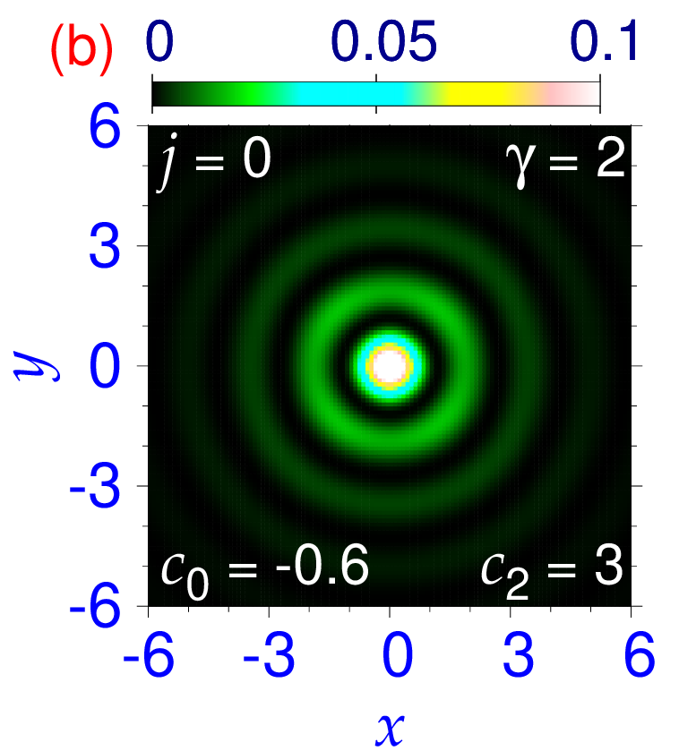
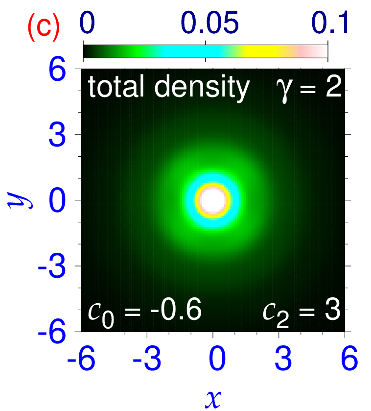
Figure 3: Contour plot of density $n_{j}$ of a $(\mp 1,0,\pm 1)$-type multi-ring spin-1 Rashba or Dresselhaus SO-coupled BEC soliton for components (a) $j=\pm 1$, (b) $j=0$ and (c) total density.

First, we consider $(\mp 1,0,\pm 1)$-type solitons for small $\gamma$ ($\gamma\lessapprox 0.75$) for Rashba (upper sign) or Dresselhaus (lower sign) SO coupling. In Fig. 2 we display the contour plot of density of components (a) $j=\pm 1$, (b) $j=0$, and (c) total density of a $(\mp 1,0,\pm 1)$-type soliton for parameters $c_{0}=-1,c_{2}=3,\gamma=0.25$. The energy and density of the $(\mp 1,0,\pm 1)$-type soliton are insensitive to the variation of $c_{2}$ in the range $10>c_{2}>0$ quasi-1d12 ; quasi-2d1 . The energy of the $(\mp 1,0,\pm 1)$-type soliton in Fig. 2 is $E=-0.030$ independent of the type of SO coupling: Rashba or Dresselhaus. In Figs. 2(d)-(e) we display the contour plot of the phase of wave function components $j=\pm 1$ of the $(-1,0,+1)$-type Rashba SO-coupled soliton of Fig. 2(a) showing a phase drop of $\mp 2\pi$ under a complete rotation, indicating angular momenta of $\mp 1$ in these components. Although the densities for Rashba and Dresselhaus SO-coupled solitons are the same the corresponding phases for Dresselhaus SO-coupling are different, viz. Figs. 2(f)-(g) showing the phases of components $j=\pm 1$ of the Dresselhaus SO-coupled soliton corresponding to a phase drop of $\pm 2\pi$ under a complete rotation, indicating angular momenta of $\pm 1$ in these components. These phases are consistent with the vortex-antivortex structure of the $(\mp 1,0,\pm 1)$-type solitons for Rashba and Dresselhaus couplings.

To study multi-ring solitons for medium $\gamma$, in Fig. 3 we show the contour plot of density of components (a) $j=\pm 1$ and (b) $j=0$ and (c) total density of a $(\mp 1,0,\pm 1)$-type multi-ring soliton for Rashba or Dresselhaus SO couplings for $c_{0}=-0.6,c_{2}=3,\gamma=2$. Although, there is modulation in density of different components, the total density shows no modulation. The phases in this case (not shown) are identical to the same of the $(\mp 1,0,\pm 1)$-type soliton shown in Figs. 2(d)-(g) reflecting the same vortex-antivortex structure at the center of the respective components for Rashba or Dresselhaus SO couplings. The energy of the $(\mp 1,0,\pm 1)$-type multi-ring soliton in Fig. 3 is $E=-1.997$ for both SO couplings. The increase of $\gamma$ from Fig. 2 to Fig. 3 has increased the binding, and hence aids in forming soliton. The change in binding due to the change of $c_{0}$ from Fig. 2 to Fig. 3 is negligible in this scale. Multi-ring solitons were also investigated in a quasi-2D pseudo spin-1/2 SO-coupled BEC trapped in a radially periodic potential radper which creates the multi-ring modulation in density. However, the present radial modulation in density without any external trap is a consequence of the SO couplings.

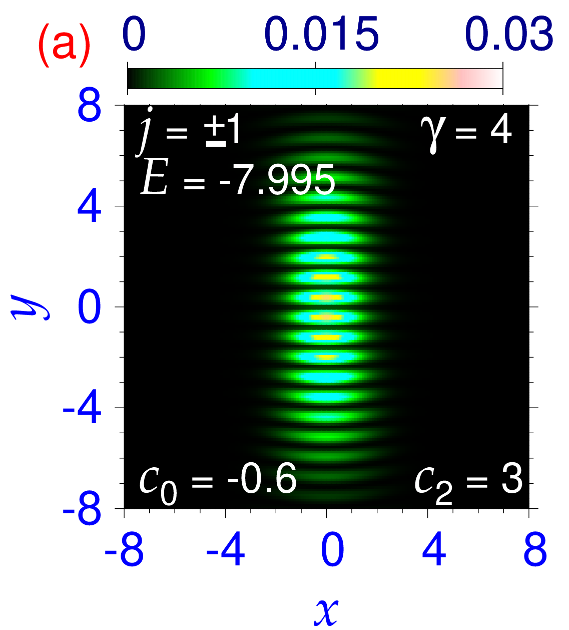
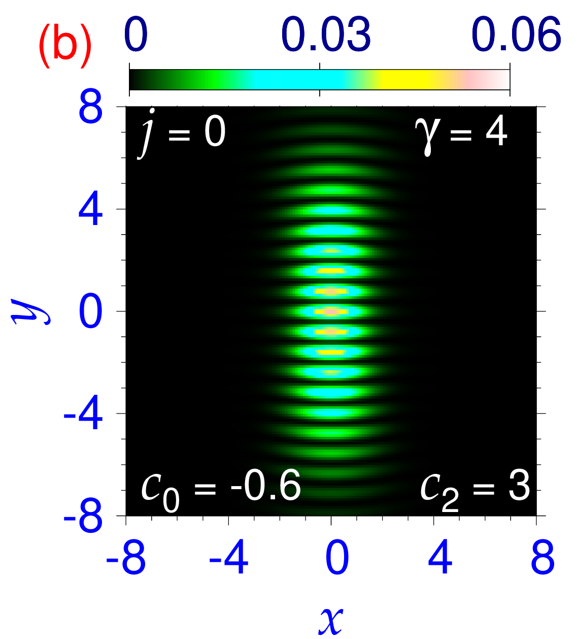
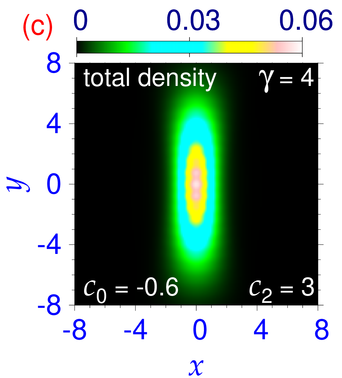
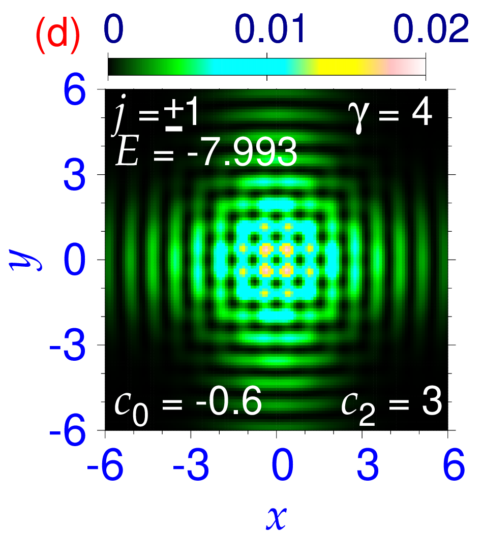
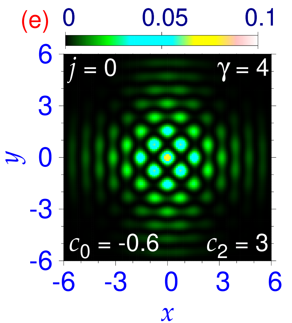
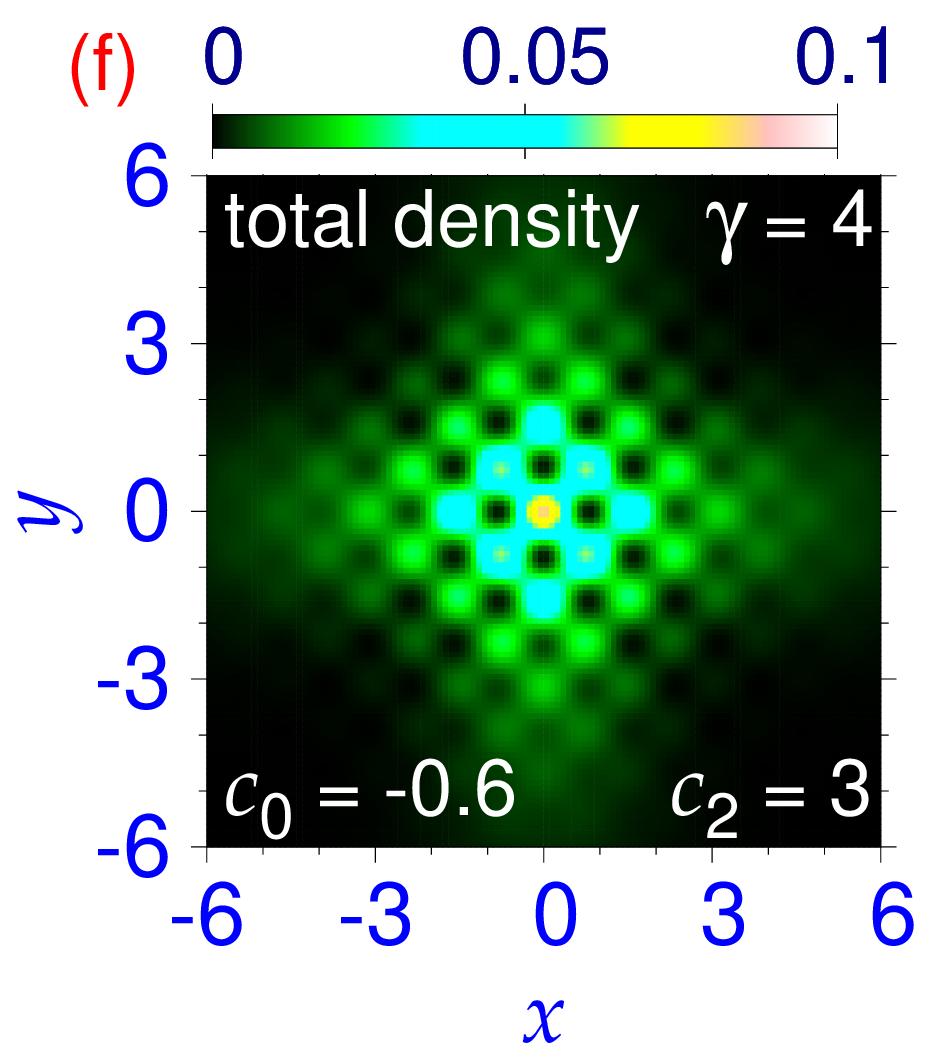
Figure 4: Contour plot of density $n_{j}$ of a stripe spin-1 Rashba or Dresselhaus SO-coupled BEC soliton of components (a) $j=\pm 1$ and (b) $j=0$ (c) the total density. The same of a super-lattice soliton of components (d) $j=\pm 1$, (e) $j=0$, and (f) the total density.

As $\gamma$ is increased, the $(\mp 1,0,\pm 1)$-type multi-ring solitons continue to exist but will not be considered further. Two new types of solitons without any vortex at the center of the components appear as quasidegenerate states: stripe and super-lattice solitons with periodic distribution of matter in $x$ and/or $y$ directions. The single particle Hamiltonian (1) should have solutions of the plane wave form $\exp(\pm i\alpha\gamma x)\otimes\exp(\pm i\beta\gamma y)$, where $\alpha$ and $\beta$ are constants. In the presence of interaction ($c_{0},c_{2}\neq 0$), the solution will be a superposition of such plane wave solutions leading to a periodic variation of density in the form $\sin^{2}(\alpha\gamma x)$, $\cos^{2}(\beta\gamma y)$, $\sin^{2}(\alpha\gamma x)\sin^{2}(\beta\gamma y)$ etc. appropriate for stripe or lattice solitons. This has been demonstrated in details for quasi-1D solitons quasi-1d1 , the same of the present quasi-2D solitons will be the subject of a future investigation. The period of the lattice or stripe increses as $\gamma$ is reduced. For small $\gamma$, the size of the soliton is smaller than this period and the periodic pattern in density is not possible. In Fig. 4 we illustrate a quasi-2D stripe soliton for $c_{0}=-0.6,c_{2}=3,$ and $\gamma=4$ through a contour plot of density of components (a) $j=\pm 1$, (b) $j=0$, and (c) total density, obtained by imaginary-time propagation using an initial localized wave function modulated by appropriate stripes in form $\sin(\gamma x)$ and $\cos(\gamma x)$ for $j=\pm 1$ and 0 components. Although, there is a stripe pattern in density in this case, the positions of maxima in components $j=\pm 1$ coincide with the minima in component $j=0$ due to a phase separation among the components, thus resulting in a total density without modulation. In Fig. 4 the super-lattice soliton for the same set of parameters is displayed through a contour plot of density of components (d) $j=\pm 1$, (e) $j=0$, and (f) total density, obtained by imaginary-time propagation using the converged wave function of Fig. 3 as the initial state. The distribution of matter on a 2D square lattice is prominent in the total density plot of Fig. 4(f) 2020 . For the same set of parameters, the stripe soliton of energy $E=-7.995$ and the super-lattice soliton of energy $E=-7.993$ are almost degenerate states with the stripe solitons having slightly smaller energy.

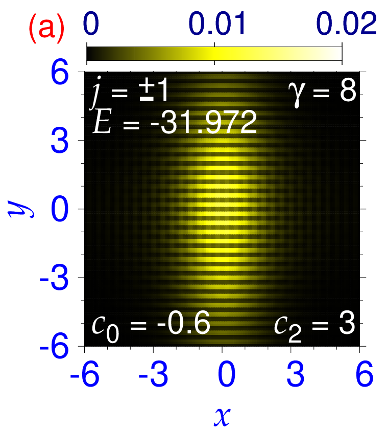
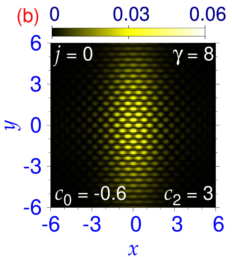
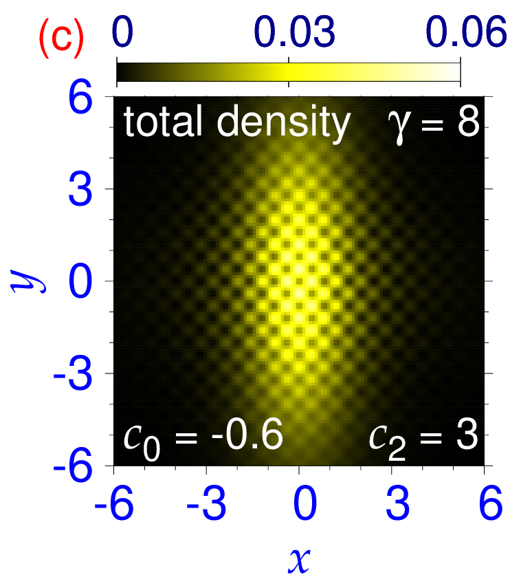
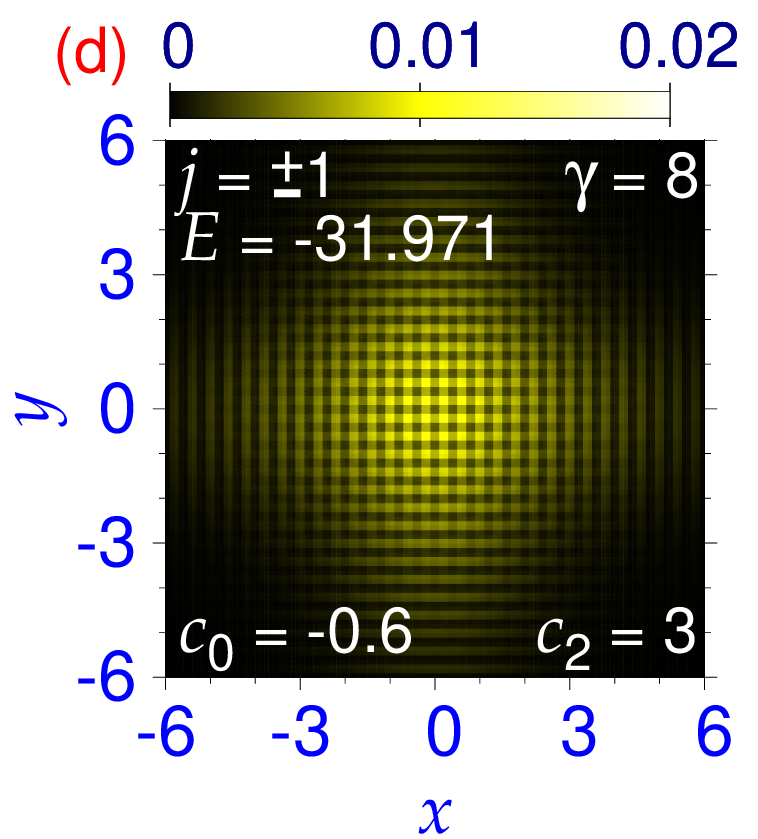
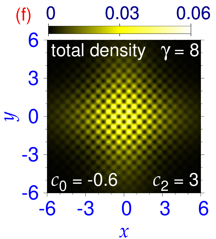
Figure 5: Contour plot of density $n_{j}$ of a super-lattice spin-1 Rashba or Dresselhaus SO-coupled BEC soliton (with a periodic stripe in $j=\pm 1$) for components (a) $j=\pm 1$, (b) $j=0$, and (c) the total density. The same of a super-lattice soliton with a square-lattice pattern in components (d) $j=\pm 1$, (e) $j=0$, and (f) the total density.

As $\gamma$ is further increased, the stripe solitons become super-lattice solitons with 2D square-lattice structure in total density. In Fig. 5 we display the contour plot of density of such a super-lattice soliton of components (a) $j=\pm 1$, (b) $j=0$, (c) total density for parameters $c_{0}=-0.6,c_{2}=3$, and $\gamma=8$. In this case, the component densities of Fig. 5(a) $(j=\pm 1)$ continue to possess a 1D stripe pattern but the total density in Fig. 5(c) and the density of the $j=0$ component in Fig. 5(b) develop a prominent 2D square-lattice structure 2020 . The component densities as well as the total density of a super-lattice soliton with 2D square-lattice structure in both are displayed in Fig. 5 for (d) $j=\pm 1$, (e) $j=0$, and (f) the total density. These two types of super-lattice solitons have practically the same energy: $E=-31.972$ and $-31.971$, respectively.

To demonstrate the dynamical stability of the solitons, we consider the stripe and the super-lattice solitons of Fig. 4 and subject the corresponding imaginary-time wave functions to real-time propagation during 100 units of time after changing $c_{2}$ from 3 to 4. The resultant density of the stripe soliton is displayed in Fig. 6 for components (a) $j=\pm 1$, (b) $j=0$, and (c) total density. The same for the super-lattice soliton are shown in Figs. 6(d)-(f). Although the root-mean-square sizes and energy were oscillating (different energies in Figs. 4 and 6) during real-time propagation, the periodic pattern in total density survived at $t=100$. If the solitons were not dynamically stable, the small numerical deviation due to a change of $c_{2}$ from 3 to 4 would have destroyed the periodic pattern in density.

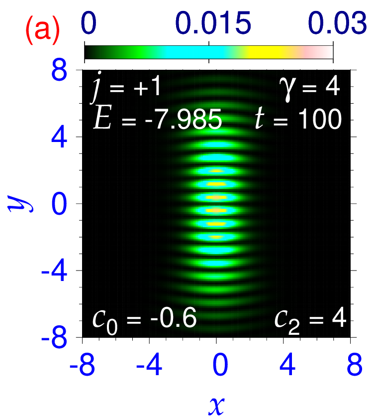
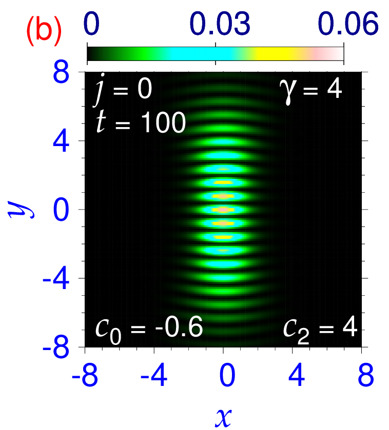
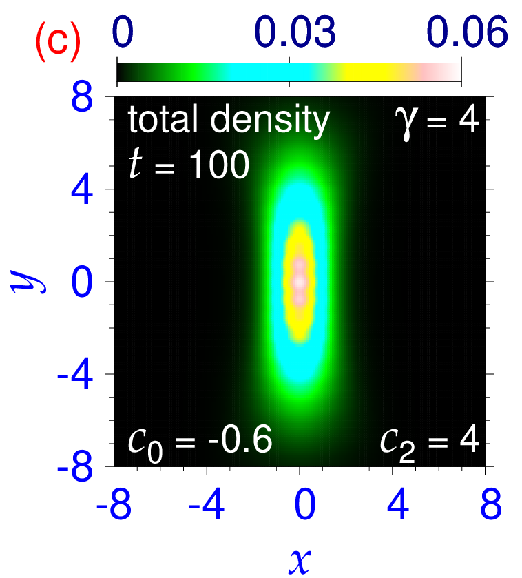
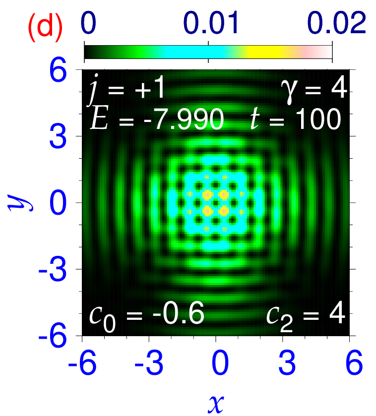
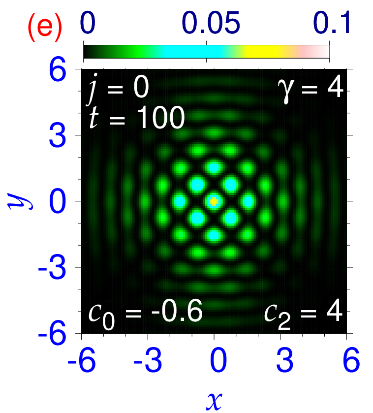
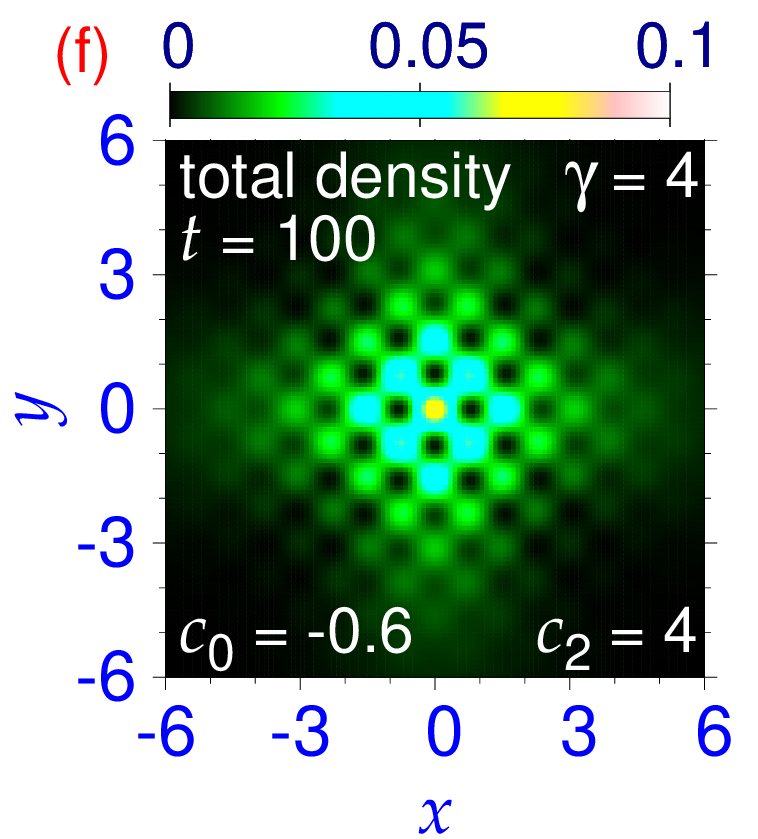
Figure 6: Contour plot of density of a stripe BEC soliton, of Fig. 4(a)-(c), of components (a) $j=\pm 1$, (b) $j=0$ and (c) the total density, after real-time propagation at time $t=100$ upon a change of $c_{2}$ from 3 to 4 at $t=0$. The same of a super-lattice soliton, of Fig. 4(d)-(f), of components (d) $j=\pm 1$, (e) $j=0$ and (f) the total density.

At a finite temperature, there will be a thermal cloud outside the super-fluid soliton and the present study at zero temperature may require corrections rmp . For ultra-low-density scalar BEC solitons r2 ; r3 , the experimental result agree for the critical number of atoms in a ⁸⁵Rb soliton at low temperature is in excellent agreement with that derived from the zero-temperature GP equation arnaldo with an estimated error of less than $1\%$. As the present solitons are also of ultra-low density with very small $|c_{0}|$, the finite-temperature corrections in an experiment are expected to be small. Hence we do not believe the finite-temperature correction to be so large as to invalidate the general findings of this study.

In the pseudo spin-1/2 SO-coupled quasi-2D BEC only stripe state was found sinha . In the quasi-2D spin-1 case, in this study, we find both stripe and 2D square lattice states. However, in a quasi-2D spin-1 BEC we could not find any super-lattice state for an equal mixture of Rashba and Dresselhaus couplings, which is a simpler 1D coupling. Preliminary studies indicate that in the quasi-2D spin-2 case there could be formation of stripe, square lattice and hexagonal lattice sandeep states. It seems that a more intricate SO coupling with an increased number of wave function components is responsible for a diverse type of super-lattice states.

We demonstrated new types of dynamically stable solitons in a Rashba or Dresselhaus SO-coupled spin-1 quasi-2D untrapped spinor antiferromagnetic ($c_{2}>0$) BEC for medium and large SO-coupling strengths $\gamma$. For medium $\gamma$, $(\mp 1,0,\pm 1)$-type multi-ring solitons are found for Rashba and Dresselhaus SO couplings. As $\gamma$ is increased, stripe and super-lattice solitons are found, where matter is distributed either in stripe form with maxima and minima or on a square quasi-2D lattice. The total density of the stripe soliton has no density modulation, whereas that of the super-lattice soliton shows a 2D square lattice pattern, viz. Fig. 4 for $\gamma=4$. As $\gamma$ is further increased, the stripe solitons become super-lattice solitons, viz. Figs. 5(a)-(c) for $\gamma=8$, where the total density exhibits a 2D periodic structure on a square lattice. The spontaneous formation of a 2D square-lattice structure in the total density of super-lattice solitons is remarkable in being a trap-less super-fluid system showing crystallization behavior. These super-lattice solitons are dynamically robust and deserve further theoretical and experimental investigation.

- (1) Y. S. Kivshar and B. A. Malomed, Rev. Mod. Phys. 61, 763 (1989); F. K. Abdullaev, A. Gammal, A. M. Kam- chatnov, and L. Tomio, Int. J. Mod. Phys. B 19, 3415 (2005).
- (2) K. E. Strecker, G. B. Partridge, A. G. Truscott, and R. G. Hulet, Nature (London) 417, 150 (2002); L. Khaykovich, F. Schreck, G. Ferrari, T. Bourdel, J. Cubizolles, L. D. Carr, Y. Castin, and C. Salomon, Science 256, 1290 (2002).
- (3) S. L. Cornish, S. T. Thompson, and C. E. Wieman, Phys. Rev. Lett. 96, 170401 (2006).
- (4) V. M. Pérez-García, H. Michinel, and H. Herrero, Phys. Rev. A 57, 3837 (1998).
- (5) R. Y. Chiao, E. Garmire, and C. H. Townes, Phys. Rev. Lett. 13, 479 (1964).
- (6) J. Stenger, S. Inouye, D. M. Stamper-Kurn, H.-J. Miesner, A. P. Chikkatur, W. Ketterle, Nature (London) 396, 345 (1998).
- (7) J. Dalibard, F. Gerbier, G. Juzeliunas, P. Öhberg, Rev. Mod. Phys. 83, 1523 (2011).
- (8) V. Galitski and I. B. Spielman, Nature (London) 494, 49 (2013).
- (9) G. Dresselhaus, Phys. Rev. 100, 580 (1955).
- (10) E. I. Rashba, Fiz. Tverd. Tela 2, 1224 (1960); [English Transla.: Sov. Phys. Solid State 2, 1109 (1960).]
- (11) Y.-J. Lin, K. Jiménez-García, I. B. Spielman, Nature (London) 471, 83 (2011).
- (12) J. Li, W. Huang, B. Shteynas, S. Burchesky, F. C. Top, E. Su, J. Lee, A. O. Jamison, and W. Ketterle, Phys. Rev. Lett. 117, 185301 (2016).
- (13) D. Campbell, R. Price, A. Putra, A. Valdés-Curiel, D. Trypogeorgos, and I. B. Spielman, Nat. Commun. 7, 10897 (2016).
- (14) V. Achilleos, D. J. Frantzeskakis, P. G. Kevrekidis, and D. E. Pelinovsky, Phys. Rev. Lett. 110, 264101 (2013).
- (15) H. Sakaguchi, B. Li, and B. A. Malomed, Phys. Rev. E 89, 032920 (2014); H. Sakaguchi and B. A. Malomed, Phys. Rev. E 90, 062922 (2014).
- (16) Y.-C. Zhang, Z.-W. Zhou, B. A. Malomed, and H. Pu, Phys. Rev. Lett. 115, 253902 (2015).
- (17) V. E. Lobanov, Y. V. Kartashov, and V. V. Konotop Phys. Rev. Lett. 112, 180403 (2014).
- (18) Y. V. Kartashov and D. A. Zezyulin, Phys. Rev. Lett. 122, 123201 (2019).
- (19) Y. V. Kartashov and V. V. Konotop, Phys. Rev. Lett. 125, 054101 (2020).
- (20) S. Gautam and S. K. Adhikari, Phys. Rev. A 91, 063617 (2015).
- (21) S. Gautam and S. K. Adhikari, Phys. Rev. A 95, 013608 (2017).
- (22) S. Gautam and S. K. Adhikari, Phys. Rev. A 97, 013629 (2018).
- (23) T. Mizushima, K. Machida, T. Kita, Phys. Rev. Lett. 89, 030401 (2002); T. Mizushima, K. Machida, T. Kita, Phys. Rev. A 66, 053610 (2002).
- (24) E.P. Gross, Phys. Rev. 106, 161 (1957); A. F. Andreev and I. M. Lifshitz, Zurn. Eksp. Teor. Fiz. 56, 2057 (1969) [English Transla.: Sov. Phys. JETP 29, 1107 (1969)]; A. J. Leggett, Phys. Rev. Lett. 25, 1543 (1970); G. V. Chester, Phys. Rev. A 2, 256 (1970); M. Boninsegni and N. V. Prokof’ev, Rev. Mod. Phys. 84, 759 (2012); V. I. Yukalov, Phys. 2, 49 (2020).
- (25) E. Kim and M. H. W. Chan, Nature (London) 427, 225 (2004); S. Balibar, Nature (London) 464, 176 (2010).
- (26) R. Bombin, J. Boronat, and F. Mazzanti, Phys. Rev. Lett. 119, 250402 (2017); F. Cinti and Massimo Boninsegni, J. Low Temp. Phys. 196, 413 (2019); Zhen-Kai Lu, Yun Li, D. S. Petrov, and G. V. Shlyapnikov, Phys. Rev. Lett. 115, 075303 (2015); N. Y. Yao, C. R. Laumann, A. V. Gorshkov, S. D. Bennett, E. Demler, P. Zoller, and M. D. Lukin Phys. Rev. Lett. 109, 266804 (2012); K. Góral, L. Santos and M. Lewenstein, Phys. Rev. Lett. 88, 170406 (2002); B. Capogrosso-Sansone, C. Trefzger, M. Lewenstein, P. Zoller, and G. Pupillo, Phys. Rev. Lett. 104, 125301 (2010).
- (27) F. Böttcher, J.-N. Schmidt, M. Wenzel, J. Hertkorn, M. Guo, T. Langen, and T. Pfau, Phys. Rev. X 9, 011051 (2019); F. Cinti and M. Boninsegni, J. Low Temp. Phys. 196, 413 (2019); J. Hertkorn, F. Böttcher, M. Guo, J. N. Schmidt, T. Langen, H. P. Büchler, and T. Pfau, Phys. Rev. Lett. 123, 193002 (2019); L. Tanzi, E. Lucioni, F. Famà, J. Catani, A. Fioretti, C. Gabbanini, R. N. Bisset, L. Santos, and G. Modugno, Phys. Rev. Lett. 122, 130405 (2019); L. Chomaz, D. Petter, P. Ilzhöfer, G. Natale, A. Trautmann, C. Politi, G. Durastante, R. M. W. van Bijnen, A. Patscheider, M. Sohmen, M. J. Mark, and F. Ferlaino, Phys. Rev. X 9, 021012 (2019); G. Natale, R. M. W. van Bijnen, A. Patscheider, D. Petter, M. J. Mark, L. Chomaz, and F. Ferlaino, Phys. Rev. Lett. 123, 050402 (2019).
- (28) J.-R. Li, J. Lee, W. Huang, S. Burchesky, B. Shteynas, F. Ç. Top, A. O. Jamison, and W. Ketterle, Nature (London) 543, 91 (2017).
- (29) Y. Li, G. I. Martone, L. P. Pitaevskii, and S. Stringari, Phys. Rev. Lett. 110, 235302 (2013).
- (30) T.-L. Ho and S. Zhang, Phys. Rev. Lett. 107, 150403 (2011); R. Liao, Phys. Rev. Lett. 120, 140403 (2018).
- (31) S. Sinha, R. Nath, and L. Santos, Phys. Rev. Lett. 107, 270401 (2011).
- (32) A. Putra, F. Salces-Carcoba, Y. Yue, S. Sugawa, and I. B. Spielman, Phys. Rev. Lett. 124, 053605 (2020).
- (33) In this figure the overlapping in-phase modulations in the spin-up and down components add up to a periodic modulation in total density.
- (34) The name super-solid does not appear in Ref. [31]. The term super-solid in this context was emphasized later in Refs. stripe ; 2020 .
- (35) L. Salasnich, A. Parola, L. Reatto, Phys. Rev. A 65, 043614 (2002).
- (36) E. P. Gross, Nuovo Cim. 20, 454 (1961); L.P. Pitaevskii, Zurn. Eksp. Teor. Fiz. 40, 646 (1961)[English Transla.: Sov. Phys. JETP. 13, 451 (1961)].
- (37) V. I. Yukalov, Laser Phys. 28, 053001 (2018); S. Gautam, S. K. Adhikari, Phys. Rev. A 92, 023616 (2015).
- (38) Y. Kawaguchi, M. Ueda, Phys. Rep. 520, 253 (2012).
- (39) R. Ravisankar, D. Vudragović, P. Muruganandam, A. Balaž, and S. K. Adhikari, Comput. Phys. Commun. 259, 107657 (2021); P. Muruganandam and S. K. Adhikari, Comput. Phys. Commun. 180, 1888 (2009); D. Vudragović, I. Vidanović, A. Balaž, P. Muruganandam, S. K. Adhikari, Comput. Phys. Commun. 183, 2021 (2012); L. E. Young-S., P. Muruganandam, S. K. Adhikari, V. Lončar, D. Vudragović, A. Balaž, Comput. Phys. Commun. 220, 503 (2017).
- (40) S. Gautam and S. K. Adhikari, Laser Phys. Lett. 12, 045501 (2015).
- (41) F. Dalfovo, S. Giorgini, L. P. Pitaevskii, and S. Stringari, Rev. Mod. Phys. 71, 463 (1999).
- (42) N. R. Claussen, S. J. J. M. F. Kokkelmans, S. T. Thompson, E. A. Donley, E. Hodby, and C. E. Wieman, Phys. Rev. A 67, 060701(R) (2003).
- (43) A. Gammal, T. Frederico, and L. Tomio, Phys. Rev. A 64, 055602 (2001).
- (44) S. Gautam and S. K. Adhikari, unpublished.