Abstract

Within the finite-time-path out-of-equilibrium quantum field theory (QFT), we calculate direct photon emission from early stages of heavy ion collisions, from a narrow window, in which uncertainty relations are still important and they provide a new mechanism for production of photons. The basic difference with respect to earlier calculations, leading to diverging results, is that we use renormalized QED of quarks and photons. Our result is a finite contribution that is consistent with uncertainty relations.

3 4 44 Received: 15 July 2020; Accepted: 7 October 2020; Published: 20 October 2020 yes yes Direct Photons from Hot Quark Matter in Renormalized Finite-Time-Path QED Ivan Dadić ^1,∗, Dubravko Klabučar ² and Domagoj Kuić ¹ Ivan Dadić , Dubravko Klabučar and Domagoj Kuić Correspondence: dadic@irb.hr

1 Introduction

Heavy ion collisions (HIC) result in many-particle final states that carry a lot of information, which is not easy to decode Baym:2016wox ; Pasechnik:2016wkt ; David:2019wpt , including, for example, the recently emerged ‘direct photon puzzle’ David:2019wpt . Various attempts to describe HIC by theoretical means include increasingly involved approaches, such as S-matrix QFT and equilibrium, as well as out-of-equilibrium QFT Schwinger:1960qe ; Keldysh:1964ud ; KadanoffBook ; Danielewicz:1982kk ; Chou:1984es ; Rammer:1986zz ; Landsman:1986uw ; Calzetta:1986cq ; Niemi:1987pm ; Remler:1990 ; LeBellacBook ; Brown:1998zx ; Blaizot:2001nr . Finally, the fast evolving nature of HIC requires the finite-time-path description. Pertinent calculations bv ; bvhs ; devega ; bvs0 ; wbvl ; wb ; ng ; bv68 ; bvhep of production of photons from the early stage of HIC, and the heated discussion afterwards Arleo:2004gn , with the criticism on infinite energy that is released in photon yield, indicate that the subject is far from settled.

This calculation is performed in the finite-time-path (FTP) out-of-equilibrium QFT. FTP is a variation of out-of-equilibrium QFT with propagators defined through a finite-time contour. Close to our approach are the Dynamical Renormalization Group approach by Boyanovsky and collaborators bv ; bvhs , and Millington’s and Pilaftsis’ formulation Millington:2012pf ; Millington:2013qpa of non-equilibrium thermal field theory. Specific to our approach is the use of the retarded-advanced ($R$-$A$) basis, where the Keldysh ($K$) propagator ($D_{K}$) is also separated into its advanced and retarded parts ($D_{K,A}$ and $D_{K,R}\,,$ respectively). The formalism Dadic:1999bp ; Dadic:2002wv ; Dadic:2009zz ; Dadic:2019lmm is equivalent to the approach of Boyanovsky and De Vega bv ; nevertheless, in the evaluation of production of direct photons, the difference is that we are calculating in the energy-momentum representation and avoid early approximations and simplifications.

Only having perturbative QED interactions, photons are “clean” probes of the quark-gluon plasma (QGP), regardless of whether it is in the regime of nonperturbative or perturbative QCD. For temperatures that are not much higher than the (pseudo)critical temperature $T_{c}$ of the crossover transition, QGP is still strongly coupled for sure Baym:2016wox ; Pasechnik:2016wkt . However, there are claims Paquet:2015lta that, in photon production calculations, one can rely on perturbative QCD corrections. These claims are supported by lattice around and even below $T\sim 1.3T_{c}$ Ghiglieri:2016tvj . Even in references that stress the nonperturbative character of QCD significantly above $T_{c}$, QGP begins approaching its perturbative regime beyond $T\sim 2T_{c}$ Ding:2015ona , i.e., above (250–300) MeV. Moreover, observables that are dominated at high $T$ by quark rather than gluon contributions seem to approach perturbative behavior earlier Ding:2015ona , and the fermionic sector is weakly coupled for $T>300$ MeV Haque:2014rua . Thus, in the very early, pre-equilibrium phase, where temperature $T$ is not even defined, but the average energy per particle is high enough, i.e., higher than $k_{B}\times 300$ MeV, one can assume that the asymptotic QCD regime is reached, and asymptotic freedom makes quarks move around quasi-free. Subsequently, in the lowest approximation, one can neglect the dressing of quark-photon vertices by QCD interactions. In particular, the fully dressed quark-photon vertex in the vacuum polarization diagram of photons is replaced by the free quark-photon vertex $\,e_{\rm q}\,\gamma_{\mu}\,$, as in Figure 1.

In any case, in the high-energy phase, various flavors of quarks and antiquarks will be present and the energy of the heavy-ion collisions determine the number of active quark flavors. With expansion and cooling, the average energy per particle drops continuously until the phase in which quarks became confined, and the system turns into hadron matter, where strong interactions dominate. Finally further expansion produces interparticle distances bigger than the range of strong interactions, and  the system decays to individual particles.

One expects the production of highest energy photons in the early stage of HIC. The mechanism that is discussed in this paper only produces photons in this stage.

The photons, which do not interact strongly with quarks and gluons, escape relatively easily, carrying the valuable information on early stage of HIC. In this stage, the uncertainty relations allow large energy uncertainty producing fast oscillations.

The Dyson–Schwinger equation for photon $D_{K,R}$ propagator requires renormalization Giambagi:1972 ; Thooft:1972 ; Ashmore:1972 ; Cicuta:1972 ; Wilson:1973 ; Kislinger:1976 ; Donoghue:1983 ; Johansson:1986 ; Kobes:1989 ; Keil:1989 ; LeBellac:1990 ; Elmfors:1992 ; Eijck:1996 ; Chapman:1997 ; Nakkagawa:1997 ; Baacke:1998 ; Esposito:1998 ; Knoll:2002 ; Jakovac:2005 ; Arrizabalaga:2007 ; Blaizot:2007 ; Blaizot:2015 ; RyderBook of divergent $\Pi_{R}$ and $\Pi_{A}$ vacuum polarizations. The related problems emerging are an additional energy-not-conserving vertex and regularized $\Pi_{R}$ not vanishing as $|p_{0}|\rightarrow\infty$ (potentially breaking causality). They are solved in full analogy to the case of out-of-equilibrium $\lambda\phi^{3}$ field theory, as discussed in Dadic:2019lmm . The solution involves: energy integrations performed, while $d<4$, subtractions in $\Pi_{F}$, and “reparation” of causality in the products, like $D_{R}\Pi_{R}$ or $\Pi_{R}D_{R}$ and analogously for $\Pi_{A}$.

Our final result is finite. In particular, the contributions that contain initial distribution functions of quarks and/or antiquarks are finite. The calculation is straightforward, but one should notice how potentially pinching term turns into the contribution linear in time $t$.

Prospects for further development are discussed.

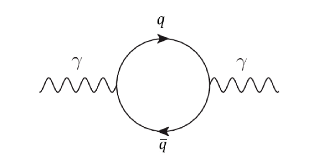
Figure 1: The lowest-order correction to the vacuum polarization $\Pi^{\rho\sigma}$ of photons, due to quarks of the flavor $q$.

2 Direct Photon Production

At the time $t$, number density of detected photons of the polarization $e$ $(e=e_{0},e_{1},e_{2},e_{3})$ and momentum $\vec{p}$ is:

$$\langle\,N_{\vec{p},e,t}\,\rangle\,=\,(2\pi)^{3}{d{\cal N}_{e}\over d^{3}x\,d^{3}p}\,,$$ (1)

where $d{\cal N}_{e}$ is the number of photons of the polarization $e$ inside the differential volumes $d^{3}x$ and $d^{3}p$ of the coordinate and momentum spaces.

The number density is connected to the equal time limit of the $K$ (Keldysh) component of the dressed photon propagator ${\cal D}_{\mu\nu}$ (for simplicity, we use Feynman gauge):

$$2\langle\,N_{\vec{p},e,t}\,\rangle+1\,=\,-\,{\omega_{p}\over 2\pi}\lim_{t_{1}\rightarrow t}\int dp_{0}{\cal D}_{K,t_{1},t,\mu\nu}(p)e^{\mu}e^{*\nu}\,.$$ (2)

There are various definitions Blaizot:2001nr ; wbvl ; Garbrecht:2002pd of number density based on the product of creation and annihilation operators, $a^{\dagger}$ and $a$. They are mostly equivalent, at least at low orders. Our definition is adapted to the presently used formalism, as the dressed Keldysh propagator ${\cal D}_{K}={\cal D}_{K,R}-{\cal D}_{K,A}$ is easily calculated from perturbation expansion for matrix propagators (${\cal D}_{ij}$) as well as from Dyson–Schwinger equation.

As expected, at the lowest order of the perturbation expansion, it is

$$2\langle\,N_{\vec{p},e,t}^{0}\,\rangle+1\,=\,2\,f_{e}(\vec{p})\,+\,1\,,$$ (3)

where the function $f_{e}(\vec{p})$ is the initial ($t=0$) distribution function for photons. However, they freely escape from the medium after they are created in the collision, and  do not accumulate in the quark medium created by the collision of nucleons. Thus, we set $f_{e}(\vec{p})=0$ as the initial condition. We are only interested in the photons from the early quark phase.

The initial distributions of quarks ($n_{+}(\vec{p})$) and of antiquarks ($n_{-}(\vec{p})$) are the input functions for out-of-equilibrium field theory, where they are independent. All of the initial distribution functions ($f_{\rm i}=f_{e},n_{\pm}$) have to satisfy the following conditions: $\int\,d^{3}pf_{\rm i}(\vec{p})<\infty$, $\int d^{3}p\,\omega_{\vec{p}}\,f_{\rm i}(\vec{p})<\infty$, saying, respectively, that the probability and the average energy are finite. There is no condition regarding analyticity.

In principle, highly anisotropic situations can be considered. Nevertheless, in many applications, the basic assumption is that the system is close to equilibrium and, in such cases, a natural choice for $n_{\pm}$ is the Fermi–Dirac distribution function, which is isotropic:

$$n_{\pm}(\vec{p})\,\to\,n_{\pm}(\omega_{p})\,=\,{\,1\over e^{(\omega_{p}-\mu_{\pm})/T}+1\,}~{}.$$ (4)

This was the choice of Wang and Boyanovsky bv , and we will also use it when we compare our result to theirs.

Even for out-of-equilibrium situations, some phenomenologists speak loosely about temperature $T$ and chemical potential $\mu$ as the characterization of average single particle energy and particle number. We expect that, by fitting the measured direct photon data, one can extract some knowledge regarding $f(\vec{p})$ function.

In comparison with the cross-section, which is proportional to time derivative of exclusive number of particles, the number of “detected” photons is inclusive. It is the density number of photons (i.e., “gain minus loss”) detected until the time $t$ (yield).

In order to calculate the first nontrivial order contributions to $\langle\,N_{\vec{p},e,t}\,\rangle$ in (2), for ${\cal D}_{K,t_{1},t_{2},\mu\nu}(p)$, we use Dyson–Schwinger Equations (5), where time and momenta variables are suppressed for compactness, and where $*$ denotes the convolution product defined in Appendix A by Equation (17):

$$\begin{array}[]{l}{\cal D}_{\mu\nu,K}\,=\,{D}_{\mu\nu,K}+i[D_{\mu\rho,R}*\Pi^{\rho\sigma}_{K}*{D}_{\sigma\nu,A}+D_{\mu\rho,R}*\Pi^{\rho\sigma}_{R}*{D}_{\sigma\nu,K}+D_{\mu\rho,K}*\Pi^{\rho\sigma}_{A}*{D}_{\sigma\nu,A}]\,\,,\cr\\ \Pi^{\rho\sigma}_{K}\,=\,-\Pi^{\rho\sigma}_{K,R}+\Pi^{\rho\sigma}_{K,A}\,\,,\end{array}$$ (5)

where all vacuum polarizations $\Pi^{\rho\sigma}$ are of the lowest order (one loop), as in Figure 1.

The expression (5) contains two types of problems: divergences Dadic:2019lmm and vertices Dadic:1998yd ; Dadic:1999bp ; Dadic:2002wv ; Dadic:2009zz .

The divergences are contained in $\Pi^{\rho\sigma}_{R}$ and $\Pi^{\rho\sigma}_{A}$. These divergences are descendants of the divergence of the Feynman vacuum polarization $\Pi^{\rho\sigma}_{F}$. In the dimensional regularization at $d<4$, they are regulated (i.e., finite) and can be subtracted. Other vacuum polarizations $\Pi^{\rho\sigma}_{K}$ are expected to be finite.

Vertices are of the following three types:

1. Vertices with at least one outgoing retarded propagator or incoming advanced propagator. Energy conservation is achieved by simple integration over the energy of such propagator, by closing the contour from above for the retarded and from below for the advanced propagator. This case includes the cases when there are more than one such propagators connecting the same vertex. In this case, the loop integrals should not diverge. The convolution product $*$ containing them turns into the usual algebraic product. Examples: the vertex between the two-point functions $D_{\mu\rho,R}$ and $\Pi^{\rho\sigma}_{K,R}$; between $\Pi^{\rho\sigma}_{K,A}$ and ${D}_{\sigma\nu,A}$; between $\Pi^{\rho\sigma}_{R}$ and $D_{\mu\rho,K,R}$; between ${D}_{\sigma\nu,K,A}$ and $\Pi^{\rho\sigma}_{A}$, as they appear in the Dyson–Schwinger equation terms $D_{\mu\rho,R}*\Pi^{\rho\sigma}_{R}*{D}_{\sigma\nu,K}+D_{\mu\rho,K}*\Pi^{\rho\sigma}_{A}*{D}_{\sigma\nu,A}$.

2. Vertices without any outgoing retarded propagator or incoming advanced propagator. They are lower in time than neighboring vertices. Closing the integration path always catches some singularities of the propagators. These terms will not conserve energy, but they oscillate in time, with high frequency. The examples are: the vertex between the two-point functions $D_{\mu\rho,R}$ and $\Pi^{\rho\sigma}_{K,A}$; between $\Pi^{\rho\sigma}_{K,R}$ and ${D}_{\sigma\nu,A}$; between $\Pi^{\rho\sigma}_{R}$ and $D_{\mu\rho,K,A}$ ; and, between ${D}_{\sigma\nu,K,R}$ and $\Pi^{\rho\sigma}_{A}$.

3. Vertices with at least one outgoing retarded propagator, or at least one incoming advanced propagator, but with two or more such propagators entering the same vertex, where the corresponding loop integral diverges. These vertices should conserve energy, but divergent integrals make them ill-defined. At $d<4$, the loop integrals are regulated, and  the usual closing of the integration contour leads to energy conservation. This make them group 1. vertices. Examples of such vertices are the ones between the two-point functions $D_{\mu\rho,R}$ and $\Pi^{\rho\sigma}_{R}$, as well as $\Pi^{\rho\sigma}_{A}$ and ${D}_{\sigma\nu,A}$. Additionally, in the case that the mentioned vertex is connected with yet another one, where this connection satisfies the condition for the group 1 vertices, the mentioned vertex immediately belongs to the group 1.

These properties lead to the simplified version of Dyson–Schwinger equation at the first order:

$$\begin{array}[]{l}{\cal D}_{\mu\nu,K}\,=\,{D}_{\mu\nu,K}+i\,[\,-D_{\mu\rho,R}\Pi^{\rho\sigma}_{K,R}*{D}_{\sigma\nu,A}+D_{\mu\rho,R}*\Pi^{\rho\sigma}_{K,A}{D}_{\sigma\nu,A}\cr\\ \qquad\qquad-D_{\mu\rho,R}\Pi^{\rho\sigma}_{R}*{D}_{\sigma\nu,K,A}+D_{\mu\rho,K,R}*\Pi^{\rho\sigma}_{A}{D}_{\sigma\nu,A}\cr\\ \qquad\qquad+D_{\mu\rho,R}\Pi^{\rho\sigma}_{R}{D}_{\sigma\nu,K,R}-D_{\mu\rho,K,A}\Pi^{\rho\sigma}_{A}{D}_{\sigma\nu,A}\,].\end{array}$$ (6)

Inserting this ${\cal D}_{\mu\nu,K}$ in Equation (2) and using the convolution product defined in Appendix A, reveals that the one-loop contribution to the photon number density is

$$\begin{array}[]{l}\langle\,N^{1}_{\vec{p},t}\,\rangle\,=\,\sum_{\mu,\nu}g^{\mu\nu}{\omega_{p}\over 4\pi}i\int dp_{01}dp_{02}dp_{0}P_{t}(p_{0},{p_{01}+p_{02}\over 2}){i\over 2\pi}{e^{-it(p_{01}-p_{02}+i\epsilon)}-1\over p_{01}-p_{02}+i\epsilon}\cr\\ \times[\,-D_{\mu\rho,R}(p_{01},\vec{p})\Pi^{\rho\sigma}_{K,R}(p_{01},\vec{p}){D}_{\sigma\nu,A}(p_{02},\vec{p})-D_{\mu\rho,R}(p_{01},\vec{p})\Pi^{\rho\sigma}_{R}(p_{01},\vec{p}){D}_{\sigma\nu,K,A}(p_{02},\vec{p})\cr\\ \quad+D_{\mu\rho,R}(p_{01},\vec{p})\Pi^{\rho\sigma}_{K,A}(p_{02},\vec{p}){D}_{\sigma\nu,A}(p_{02},\vec{p})+D_{\mu\rho,K,R}(p_{01},\vec{p})\Pi^{\rho\sigma}_{A}(p_{02},\vec{p}){D}_{\sigma\nu,A}(p_{02},\vec{p})\cr\\ \quad+D_{\mu\rho,R}(p_{01},\vec{p})\Pi^{\rho\sigma}_{R}(p_{01},\vec{p})D_{\sigma\nu,K,R}(p_{02},\vec{p})-D_{\mu\rho,K,A}(p_{01},\vec{p})\Pi^{\rho\sigma}_{A}(p_{02},\vec{p})D_{\sigma\nu,A}(p_{02},\vec{p})\,]~{}.\end{array}$$ (7)

The last two terms ($RRR$ and $AAA$) vanish in the limit of equal time. The function $P_{t}(p_{0},{p_{01}+p_{02}\over 2})$ is the projecting function defined in the Appendix A.

In the rest of the text, we suppress the Lorentz indices.

Next, we perform equal time limit procedure. Equal time limit of the product of two or more retarded functions vanishes, as one can, in that case, close the integration contour $dp_{0}$ in a way to catch no singularity. Such a product of advanced functions also vanishes. The diverging $\Pi_{R}$ and $\Pi_{A}$ are represented by vacuum polarizations in the matrix representation Dadic:2019lmm as

$$\begin{array}[]{l}\Pi_{j,k}=-\Pi_{K,R}+\Pi_{K,A}-\,k\,\Pi_{R}-\,j\,\Pi_{A}\qquad(i,j=1,2)\,\,,\cr\\ \Pi_{11}=\Pi_{F}-\Pi_{n_{+},n_{-},R}+\Pi_{n_{+},n_{-},A}\,\,,\cr\\ Re\Pi_{R(A),n_{\pm}=0}(p)=Re\Pi_{F}~{},\end{array}$$ (8)

where $\Pi_{n_{+},n_{-},R(A)}$ are the corrections to $\Pi_{F}$ by finite $n_{\pm}$.

Calculated at $d<4$ and regularized by subtraction of constant term, the closing the integration path over $dp_{01}$ from above shows that the subtraction term vanishes.

Integration over $dp_{0}$ removes (see Appendix A) the $P_{t}(p_{0},p^{\prime}_{0})$ projector.

In the first two terms in the square bracket in Equation (7), one can close the $dp_{02}$ integration path from above and catch only the singularities of $D_{A}$ and $D_{K,A}$. The integration over $dp_{01}$ can be closed from below with the singularities caught from $D_{R}$ and $D_{K,R}$ and from $\Pi_{R}$ and $\Pi_{K,R}$. Important to notice is that the poles of both, $D_{A}$ and $D_{K,A}$, are equal $[\bar{p}_{02}]_{1(2)}=\pm\omega_{p}+i\epsilon$, for $D_{R}$ and $D_{K,R}$ they are $[\bar{p}_{01}]_{1(2)}=\pm\omega_{p}-i\epsilon$. Singularities of $\Pi_{R}$ and $\Pi_{K,R}$ may be complicated.

In the terms with only poles of propagators, the vertex factor requires a limiting procedure

$$\lim_{\epsilon\rightarrow 0}[{e^{-it(\bar{p}_{01}-\bar{p}_{02}+i\epsilon)}-1\over\bar{p}_{01}-\bar{p}_{02}+i\epsilon}]_{\bar{p}_{01}=\bar{p}_{02}*=\pm\omega_{p}-i\epsilon}=-it.$$ (9)

The corresponding terms are growing linearly with time.

Similar, but complex conjugated, are the contributions of the last two terms in Equation (7). Thus, we obtain

$$\begin{array}[]{l}\int_{-\infty}^{\infty}dp_{0}\,{\cal D}^{1}_{K,t}(p_{0},\vec{p})\,=\,-\,{i\pi t\over 2\omega_{p}^{2}}\sum_{\lambda=\pm}[\,-\Pi_{K,R}(\lambda\omega_{p},\vec{p})+\lambda\Pi_{R}(\lambda\omega_{p},\vec{p})(1+2f_{e}(\omega_{p}))\cr\\ \qquad\qquad\qquad\qquad\qquad\qquad\qquad\quad+\,\Pi_{K,A}(-\lambda\omega_{p},\vec{p})-\lambda\Pi_{A}(-\lambda\omega_{p},\vec{p})\left(1+2f_{e}(\omega_{p})\,\right)\,]\cr\\ \qquad\qquad\qquad-\,{\pi\over 4\omega_{p}^{2}}\sum_{\lambda=\pm}{e^{-i2t\lambda\omega_{p}}-1\over\omega_{p}}\,[\,\lambda\Pi_{K,R}(\lambda\omega_{p},\vec{p})-\Pi_{R}(\lambda\omega_{p},\vec{p})(1+2f_{e}(\omega_{p}))\cr\\ \qquad\qquad\qquad\qquad\qquad\qquad\qquad+\,\lambda\Pi_{K,A}(-\lambda\omega_{p},\vec{p})-\Pi_{A}(-\lambda\omega_{p},\vec{p})(1+2f_{e}(\omega_{p}))]\cr\\ +\,{1\over\omega_{p}}\sum_{\lambda=\pm}{\cal P}\int_{cut}{dp_{0}\over p^{2}}{e^{-it(p_{0}-\lambda\omega_{p})}-1\over p_{0}-\lambda\omega_{p}}\,[\lambda Im\Pi_{K,R}(p_{0},\vec{p})+Im\Pi_{R}(p_{0},\vec{p})(1+2f_{e}(\omega_{p}))\,]\cr\\ +{1\over\omega_{p}}\sum_{\lambda=\pm}{\cal P}\int_{cut}{dp_{0}\over p^{2}}{e^{it(p_{0}-\lambda\omega_{p})}-1\over p_{0}-\lambda\omega_{p}}\,[\,\lambda Im\Pi_{K,A}(p_{0},\vec{p})-Im\Pi_{A}(p_{0},\vec{p})(1+2f_{e}(\omega_{p}))]~{},\end{array}$$ (10)

where $\cal P$ denotes the principal value of the integrals.

We use the symmetries of the one-loop vacuum polarizations to simplify the above expression

$$\begin{array}[]{l}\Pi_{K,R}(-|p_{0}|,\vec{p})=-\Pi^{*}_{K.R}(|p_{0}|,\vec{p})=\Pi^{*}_{K,A}(-|p_{0}|,\vec{p})=-\Pi_{K,A}(|p_{0}|,\vec{p}),\cr\\ \Pi_{R}(-|p_{0}|,\vec{p})=\Pi^{*}_{R}(|p_{0}|,\vec{p})=\Pi^{*}_{A}(-|p_{0}|,\vec{p})=\Pi_{A}(|p_{0}|,\vec{p})~{}.\end{array}$$ (11)

Our final result for the one-loop contribution to the photon number density is

$$\begin{array}[]{l}\langle\,N^{1}_{\vec{p},t}\,\rangle\,=\,{\omega_{p}\over 4\pi}\int_{-\infty}^{\infty}dp_{0}\,{\cal D}^{1}_{K,t}(p_{0},\vec{p})\,=\cr\\ {t\over 2\omega_{p}}[-Im\Pi_{K,R}(\omega_{p},\vec{p})+Im\Pi_{R}(\omega_{p},\vec{p})(1+2f_{e}(\omega_{p}))]\cr\\ -{1\over 4\omega_{p}^{2}}(1+2f_{e}(\omega_{p}))[(1-\cos{2t\omega_{p}})Re\Pi_{R}(\omega_{p},\vec{p})+\sin{2t\omega_{p}}Im\Pi_{R}(\omega_{p},\vec{p})]\cr\\ +{2\over\pi^{2}\omega_{p}}\,{\cal P}\int_{p_{0}>0,~{}cut}{dp_{0}\over(p_{0}^{2}-\omega_{p}^{2})^{2}}[p_{0}(1-\cos tp_{0}\cos t\omega_{p})-\omega_{p}\sin tp_{0}\sin t\omega_{p}]\cr\\ \times(1+2f_{e}(\omega_{p}))Im\Pi_{R}(p_{0},\vec{p})~{}.\end{array}$$ (12)

In Appendix C, we give the results on the vacuum polarizations that are needed in Equation (12). To evaluate it numerically, we, of course, also need the early-time distribution functions. They are presently still unknown, but we are presently considering several Ansätze proposed in literature as physically motivated “educated guesses”.

3 Discussion of the Results

Thus, we end up with four sorts of terms. One of them is just the initial particle distribution, i.e., Equation (3). As we explain after Equation (3), this “zeroth order term” is not contained in Equation (12).

3.1 Energy Conserving Terms

The terms appearing in the first square bracket in (12) are the terms from propagator poles satisfying $\bar{p}_{01}=\bar{p}_{02}^{*}$. These terms grow linearly with time (see Equation (9)). At large times, these terms would be dominating. They have the other desired properties:

1. They conserve energy.

2. They vanish for the distribution functions satisfying detailed balance principle. Indeed, the bracket from (59) in Appendix C is the defect of detailed balance in all of the channels:

   $$\begin{array}[]{l}\Theta(p_{0}-q_{0})\Theta(q_{0})[n_{+}(\omega_{p-q})n_{-}(\omega_{q})(1+f(\omega_{p}))(1-n_{+}(\omega_{p-q}))(1-n_{-}(\omega_{q}))f(\omega_{p})]\cr\\ +\Theta(q_{0}-p_{0})\Theta(-q_{0})[n_{-}(\omega_{p-q})n_{+}(\omega_{q})(1+f(\omega_{p}))(1-n_{-}(\omega_{p-q}))(1-n_{+}(\omega_{q}))f(\omega_{p})]\cr\\ +\Theta(q_{0}-p_{0})\Theta(q_{0})[(1-n_{-}(\omega_{p-q}))n_{-}(\omega_{q})(1+f(\omega_{p}))-n_{-}(\omega_{p-q})(1-n_{-}(\omega_{q}))f(\omega_{p})]\cr\\ +\Theta(p_{0}-q_{0})\Theta(-q_{0})[(1-n_{+}(\omega_{p-q}))n_{+}(\omega_{q})f(\omega_{p})\cr\\ -n_{+}(\omega_{p-q})(1-n_{+}(\omega_{q}))(1+f(\omega_{p}))(1-n_{+}(\omega_{p-q}))n_{+}(\omega_{q})f(\omega_{p})]\,].\end{array}$$ (13)

   In Equation (13), unpolarized photons are assumed; hence, no subscripts appear on their distribution functions $f(\omega_{p})$.

3. They are proportional to the lowest order Collision integral. Nevertheless, their contribution vanishes, owing to the kinematical limitations. (Otherwise, these terms would correspond to the contribution from the usual $S$-matrix formalism.)

3.2 Term Containing $Re\Pi_{R}$

The second term in Equation (12) is the term from propagator poles satisfying $\bar{p}_{01}=-\bar{p}_{02}^{*}$. Energy is not conserved in this term. The contribution containing $Re\Pi_{R}$ requires the renormalization of finite-time-path out-of-equilibrium $\phi^{3}$ QFT Dadic:2019lmm . The important points are: The vertices in the products $D_{R}*\Pi_{R}$ and $\Pi_{A}*D_{A}$ should conserve energy, but, owing to the divergences in $\Pi_{R}$ and $\Pi_{A}$, the  energy-delta function appears only if we integrate over intermediate energy while keeping $d<4$. Subsequently, thanks to properties of the convolution product Dadic:1999bp , we obtain $D_{R}*\Pi_{R}=D_{R}\Pi_{R}$ and $\Pi_{A}*{D}_{A}=\Pi_{A}{D}_{A}$.

The connection between vacuum polarizations Dadic:2019lmm , together with symmetry relations (11) gives for the vacuum parts $\Pi_{F}$ (where $n_{\pm}=0$):

$$\begin{array}[]{l}\Pi_{j,k}={1\over 2}[-\Pi_{K,R}+\Pi_{K,A}-(-1)^{k}\Pi_{R}-(-1)^{j}\Pi_{A}]~{},\qquad(j,k=1,2)~{},\cr\\ Re\Pi_{R,n_{\pm}=0}=Re\Pi_{A,n_{\pm}=0}=Re\Pi_{F}~{},\end{array}$$ (14)

where for the second line we have used the symmetries (11). Now, we obtain the renormalized value for $Re\Pi_{ren,R,f=0}(q_{0},\vec{q})=Re\Pi_{R,f=0}(q_{0},\vec{q})-CT$, where $CT$ denotes the counter-term given by the $1/(4-d)$ term in Equation (67) or Equation (68) in Appendix C.

The quantity $Re\Pi_{ren,R,f=0}(q_{0},\vec{q})$, in spite of having the label $R$, is not a true retarded function, as it does not vanish when $|q_{0}|\rightarrow\infty$. This creates a causality problem, which is repaired Dadic:2019lmm by considering the composite objects $D_{R}\Pi_{ren,R}$ and $\Pi_{ren,A}{D}_{A}$, which are retarded and advanced functions, respectively.

3.3 Cut Contributions

These are the terms from propagator poles and singularities of vacuum polarizations (principal-value contributions in Equation (12)). They are also oscillating.

While, in the first term, we may identify kinetic energy $\bar{p}_{0}$ as $\pm\omega_{p}$, in second and third term it does not make sense as there are two different values for $\bar{p}_{0}$ for each term.

At short times, all of the terms are important, as they make sure that the uncertainty relations between energy and time are satisfied.

3.4 Comparison to the Wang-Boyanovsky Result

The above expression should be compared to the Wang–Boyanovsky expression wb :

$$E\,{d{\cal N}(t)\over d^{3}p\,d^{3}x}={1\over 4\pi^{4}}\int_{-\infty}^{\infty}dp_{0}{1-\cos(p_{0}-E)t\over(p_{0}-E)^{2}}R(p_{0}),$$ (15)

where $R(p_{0})$ (in their notation, which is $f=n_{+}$ and ${\bar{f}}=n_{-}$ in our notation (4)) is

$$\begin{array}[]{l}R(p_{0})={20\pi^{2}\alpha\over 3}\int{d^{3}k\over(2\pi)^{3}}\cr\\ \left([1-(\hat{p}\hat{k})(\hat{p}\hat{q})][f(k)[1-\bar{f}(q)]\delta(p_{0}-k+q)+[1-f(k)]\bar{f}(q)]\delta(p_{0}+k-q)\right.\cr\\ \left.+[1+(\hat{p}\hat{k})(\hat{p}\hat{q})]f(k)\bar{f}(q)\delta(p_{0}-k-q)+[1-f(k)][1-\bar{f}(q)]\delta(p_{0}+k+q)\right),\end{array}$$ (16)

and where $k=|\vec{k}|$, $\hat{k}={\vec{k}\over k}$, $\hat{p}={\vec{p}\over E}$, $\vec{q}=\vec{p}-\vec{k}$, $q=|\vec{q}|$, and $\hat{q}=\vec{q}/q$.

Despite a number of common features, there are significant differences: Within the one-loop order approximation, our result is exact, while Refs. wb ; ng ignore a few terms, and make further approximations and simplifications.

In our case, the emitted photons have undefined energy in accordance with the Heisenberg uncertainty principle, similar to the findings of Millington and Pilaftsis in the context of a simple self-interacting theory of a real massive scalar field Millington:2012pf . For Equation (15), Wang and Boyanovsky claim wb that the photons are on mass shell, i.e., $p_{0}=\omega_{p}$. As the average of $\omega_{p}$ diverges Arleo:2004gn , it means infinite energy emitted in photons. In our case, the infinities are subtracted from $\Pi_{R(A)}$. It is evident that other terms are not “dangerous”.

Our result allows for the distribution functions for $q$ and $\bar{q}$ to be determined phenomenologically, i.e., not determined by $T,\mu$.

4  Conclusions

In this paper, we have calculated the production of photons from the early stage of quark gluon plasma, within the finite-time-path out-of-equilibrium QFT. The renormalization of mass divergence is analogously performed to the method that was developed for renormalization of $\lambda\phi^{3}$ out-of-equilibrium QFT Dadic:2019lmm . The result is finite. The contribution in Equation (12) oscillates (similarly as in Ref. Millington:2012pf ) in a way that is consistent with uncertainty relations between energy and time (except for energy conserving term, which vanishes for kinematical reasons). It is oscillating with the period $\propto 1/\omega_{p}$. Thus, after a few periods it will be dominated by other, higher order terms, in a lower energy-density medium, but still in pre-equilibrium. Nevertheless, it is important, as this period may provide the highest energy photons.

The result (12) inspires further investigation that is necessary to compare and predict the production of photons by numerical calculations at the lowest order and develop methods in order to obtain higher order contributions. We are in the process of performing the numerical analysis (to be published separately) aiming to investigate the following aspects:

1. Equation (12) contains renormalized $Re\Pi_{R}(\vec{p})$ linearly, whereas in usual $S$-matrix calculations it appears quadratically in higher orders of the perturbation expansion. Thus, Equation (12). at least in principle, offers a possibility, albeit challenging, to extract some information about $Re\Pi_{R}(\vec{p})$ from experiment.

2. One should distinguish the direct photon stage from the later stage in which the energy uncertainties are much smaller, but higher order perturbation contributions become more important and even start to dominate (the damping phase).

3. The early-time distributions of quarks ($n_{+}$) and antiquarks ($n_{-}$) are still unknown, and one should consider two very different situations: (a) the quarks are distributed isotropically and the probing functions could be taken as a thermalized Fermi–Dirac form like in Ref. wb . Or (b) the initial distribution of quarks may reflect the early stage distribution of nucleons. Some testing of Ansätze for the $n_{\pm}$ distributions will be necessary before reaching the final conclusion on the importance of the presented mechanism and its result (12), but we hope this will contribute to resolving the direct photon puzzle David:2019wpt .

Other developments may follow in the more ambitious direction of renormalization of the full out-of-equilibrium QED (and QCD).

Conceptualization, I.D. and D.K. (Dubravko Klabučar); Formal analysis, I.D.; Investigation, I.D., D.K. (Dubravko Klabučar) and D.K. (Domagoj Kuić); Methodology, I.D. and D.K. (Dubravko Klabučar); Software, D.K. (Domagoj Kuić); Supervision, I.D. and D.K. (Dubravko Klabučar); Validation, I.D., D.K. (Dubravko Klabučar) and D.K. (Domagoj Kuić); Writing—original draft, I.D.; Writing—review & editing, I.D., D.K. (Dubravko Klabučar) and D.K. (Domagoj Kuić). All authors have read and agreed to the published version of the manuscript.

Domagoj Kuić acknowledges partial support of the European Regional Development Fund—the Competitiveness and Cohesion Operational Programme: KK.01.1.1.06—RBI TWIN SIN, as well as the Croatian Science Foundation (HrZZ) Project No. IP-2016-06-3347. Dubravko Klabučar thanks for partial support to COST Actions CA15213 THOR and CA16214 PHAROS.

Appendix A Convolution Product

In the next step, we perform the convolution products and equal time limit.

The convolution product is defined as

$$C=A*B\Leftrightarrow C(x,y)=\int_{0}^{\infty}dzA(x,z)B(z,y)~{}.$$ (17)

In terms of Wigner transforms of projected functions Dadic:1999bp , it becomes

$$C_{X_{0}}(p_{0},\vec{p})=\int dp_{01}dp_{02}\,P_{X_{0}}(p_{0},{p_{01}+p_{02}\over 2})\,{1\over 2\pi}{ie^{-iX_{0}(p_{01}-p_{02}+i\epsilon)}\over p_{01}-p_{02}+i\epsilon}\,A_{\infty}(p_{01},\vec{p})\,B_{\infty}(p_{02},\vec{p})~{},$$ (18)

where

$$P_{X_{0}}(p_{0},p^{\prime}_{0})={1\over 2\pi}\Theta(X_{0})\int_{-2X_{0}}^{2X_{0}}ds_{0}e^{is_{0}(p_{0}-p^{\prime}_{0})}={1\over\pi}\Theta(X_{0}){\sin\left(2X_{0}(p_{0}-p^{\prime}_{0})\right)\over p_{0}-p^{\prime}_{0}},$$ (19)

and

$$e^{-is_{0}p^{\prime}_{0}}\Theta(X_{0})\Theta(2X_{0}+s_{0})\Theta(2X_{0}-s_{0})=\int dp_{0}e^{-is_{0}p_{0}}P_{X_{0}}(p_{0},p^{\prime}_{0}).$$ (20)

We have defined Dadic:1999bp the following properties: (1) the function of $p_{0}$ is analytic above (below) the real axis, (2) the function goes to zero as $|p_{0}|$ approaches infinity in the upper (lower) semi-plane. The choice above (below) and upper (lower) refers to Retarded (Advanced) functions.

In the following cases the product simplifies even further. These cases are: 1. If $A$ is advanced function and $B$ advanced, retarded, or even constant function. 2. If $B$ is retarded function and $A$ advanced, retarded, or even constant function. Then the product becomes:

$$C_{X_{0}}(p_{0},\vec{p})=\int dp_{01}P_{X_{0}}(p_{0},p_{01})A_{\infty}(p_{01},\vec{p})B_{\infty}(p_{01},\vec{p}).$$ (21)

Note that when $X_{0}\to\infty$, (19) becomes the Dirac $\delta$-function, and the convolution (21) reduces to the algebraic product: $\quad C_{\infty}(p_{0},\vec{p})\,=\,A_{\infty}(p_{0},\vec{p})\,B_{\infty}(p_{0},\vec{p})$.

However, we omit the subscript _∞ throughout this paper.

Appendix B QED—Propagators

The propagators in the covariant gauge and in the $R,A$ basis are:

$$\begin{array}[]{l}D_{\mu\nu,R}(p)=[g_{\mu\nu}-(1-a){p_{\mu}p_{\nu}\over p^{2}+2ip_{0}\epsilon}]\Delta_{R}(p),\cr\\ D_{\mu\nu,A}(p)=[g_{\mu\nu}-(1-a){p_{\mu}p_{\nu}\over p^{2}-2ip_{0}\epsilon}]\Delta_{A}(p)\cr\\ \Delta_{R(A)}(p)={i\over p^{2}\pm 2ip_{0}\epsilon}~{}.\end{array}$$ (22)

It would be interesting to obtain $D_{{\mu\nu},K}(p)$ as well as the number operator for different gauges. For simplicity we set $a=1$, obtaining Feynman gauge.

Initial densities for two transversal polarizations $e_{1,t}$, $e_{2,t}$ (linear or circular, perpendicular to $(|\vec{p}|,\vec{p})$ and mutually perpendicular) are given as $f_{1}(\vec{p})$, $f_{2}(\vec{p})$. They could be joined by density $f_{l}(\vec{p})$ for “unphysical’ longitudinal polarization $e_{l}=(0,\vec{p}/|\vec{p}|)$ and density $f_{0}(\vec{p})$ for timelike polarization $e_{0}=(1,0)$. As the longitudinal and timelike densities do not evolve with time one can fix them in a various ways. In particular one can set them equal $f_{l}(\vec{p})=f_{0}(\vec{p})$, or vanishing $f_{l}(\vec{p})=f_{0}(\vec{p})=0$. This is included in the definition of gauge. The vectors defined above, form a new basis in four vector space: $e_{0},e_{1},e_{2},e_{3}=e_{l}$ and $g_{\mu,\nu}$ is easily transformed to this basis:

$g_{ij}=\sum_{\mu,\nu}g_{\mu\nu}\,e_{i}^{*\mu}e_{j}^{\nu}$,

$g_{\mu\nu}=\sum_{i,j}g_{ij}\,e^{*i}_{\mu}e^{j}_{\nu}$,

$g_{00}=1$, $g_{11}=g_{22}=g_{33}=-1$.

Then:

$$\begin{array}[]{l}D_{\mu\nu,R}(p)=g_{\mu\nu}\,\Delta_{R}(p),\cr\\ D_{\mu\nu,A}(p)=g_{\mu\nu}\,\Delta_{A}(p),\cr\\ D_{{\mu\nu,K}}(p)=2\pi\delta(p^{2})\sum_{i,j}g_{ij}e^{*i}_{\mu}e^{j}_{\nu}[1+2f_{i}(\omega_{p})]\cr\\ =D_{{\mu\nu},K,R}(p)-D_{{\mu\nu},K,A}(p),\cr\\ D_{{\mu\nu},K,R}(p)=-D_{{\mu\nu},K,A}(-p)\cr\\ =-{p_{0}\over\omega_{p}}\sum_{i,j}g_{ij}\,e^{*i}_{\mu}\,e^{j}_{\nu}[1+2f_{i}(\omega_{p})]\,\Delta_{R}(p),\cr\\ \omega_{p}=|\vec{p}|.\end{array}$$ (23)

One needs spinor propagator (we omit the label _∞, it is understood that whenever the time label is omitted it should be _∞)

$$\begin{array}[]{l}S_{R}(p)\,=\,(p\hbox to0.0pt{\hss/\kern 1.0pt}+m)\,G_{R}(p,m)~{},\cr\\ S_{A}(p)\,=\,(p\hbox to0.0pt{\hss/\kern 1.0pt}+m)\,G_{A}(p,m)~{},\cr\\ G_{R(A)}(p,m)\,=\,{-i\over p^{2}-m^{2}\pm 2ip_{0}\epsilon}~{},\cr\\ S_{K}(p)=(P\hbox to0.0pt{\hss/\kern 1.0pt}+{mp_{0}\over\omega_{p}})\,2\pi\delta(p^{2}-m^{2})\,[1-2n(\omega_{p})]=S_{K,R}(p)-S_{K,A}(p),\cr\\ S_{K,R}(p)=-[1-2n(\omega_{p})]\,(P\hbox to0.0pt{\hss/\kern 1.0pt}+{mp_{0}\over\omega_{p}})\,G_{R}(p,m),\cr\\ S_{K,A}(p)=-[1-2n(\omega_{p})]\,(P\hbox to0.0pt{\hss/\kern 1.0pt}+{mp_{0}\over\omega_{p}})\,G_{A}(p,m),\cr\\ p\hbox to0.0pt{\hss/\kern 1.0pt}=\gamma^{\mu}p_{\mu},~{}p=(p_{0},\vec{p}),~{}P\hbox to0.0pt{\hss/\kern 1.0pt}=\gamma^{\mu}P_{\mu},~{}P=(\omega_{p},{p_{0}\over\omega_{p}}\vec{p}),~{}~{}\omega_{p}=\sqrt{\vec{p}^{2}+m^{2}\,}.\end{array}$$ (24)

$n(\omega_{p})$ is initial fermion distribution function. However, initial fermion and antifermion distribution functions can in general be different. For unequal distributions one has

$$n(p_{0},\omega_{p},\vec{p})=\Theta(p_{0})n_{+}(\omega_{p},\vec{p})+\Theta(-p_{0})n_{-}(\omega_{p},-\vec{p})~{}.$$ (25)

Now we decompose $K$-propagator into it‘s retarded and advanced part

$$\begin{array}[]{l}S_{K}(p,m)\,=\,S_{K,R}(p,m)-S_{K,A}(p,m)~{},\cr\\ S_{K,R}(p,m)\,=\,-\,G_{R}(p,m)\,L(p_{0},\vec{p})~{},\cr\\ S_{K,A}(p,m)\,=\,-\,G_{A}(p,m)\,L(p_{0},\vec{p})~{},\end{array}$$ (26)

where

$$\begin{array}[]{l}L(p_{0},\vec{p})\,=\,[1-2n_{+}(\omega_{p},\vec{p})]{p_{0}+\omega_{p}\over 2\omega_{p}}~{}2m\Lambda_{+}(\omega_{p},\vec{p})\cr\\ +[1-2n_{-}(\omega_{p},-\vec{p})]{p_{0}-\omega_{p}\over 2\omega_{p}}~{}2m\Lambda_{-}(\omega_{p},-\vec{p})~{},\cr\\ \Lambda_{+}(\omega_{p},\vec{p})={\gamma_{0}\omega_{p}-\vec{\gamma}\vec{p}+m\over 2m}~{},\cr\\ \Lambda_{-}(\omega_{p},\vec{p})={-\gamma_{0}\omega_{p}+\vec{\gamma}\vec{p}+m\over 2m}~{},\end{array}$$ (27)

where the projectors $\Lambda_{\pm}$ satisfy $\Lambda_{\pm}(\omega_{p},\vec{p})^{2}=\Lambda_{\pm}(\omega_{p},\vec{p})$, while $\Lambda_{+}(\omega_{p},\vec{p})\Lambda_{-}(\omega_{p},\vec{p})=0$, $\Lambda_{-}(\omega_{p},\vec{p})\Lambda_{+}(\omega_{p},\vec{p})=0$, and  $\Lambda_{-}(\omega_{p},\vec{p})+\Lambda_{+}(\omega_{p},\vec{p})=1$.

The above result can be rewritten as:

$$\begin{array}[]{l}S_{K,R(A)}(p)=[1-2{\bar{n}}(\omega_{p})]{i(P\hbox to0.0pt{\hss/\kern 1.0pt}+mp_{0}/\omega_{p})\over p^{2}-m^{2}\pm 2ip_{0}\epsilon}-2n_{\Delta}(\omega_{p}){i(p\hbox to0.0pt{\hss/\kern 1.0pt}+m)\over p^{2}-m^{2}\pm 2ip_{0}\epsilon},\cr\\ \bar{n}(\omega_{p})={n_{+}(\omega_{p})+n_{-}(\omega_{p})\over 2},~{}~{}n_{\Delta}(\omega_{p})={n_{+}(\omega_{p})-n_{-}(\omega_{p})\over 2}~{},\end{array}$$ (28)

We can also obtain $S_{11}$,

$$\begin{array}[]{lll}S_{11}(p)&=&{1-2{\bar{n}}(\omega_{p})\over 2}{i(P\hbox to0.0pt{\hss/\kern 1.0pt}+mp_{0}/\omega_{p})\over p^{2}-m^{2}+2ip_{0}\epsilon}+{1-2n_{\Delta}(\omega_{p})\over 2}{i(p\hbox to0.0pt{\hss/\kern 1.0pt}+m)\over p^{2}-m^{2}+2ip_{0}\epsilon}\cr\\ &-&{1-2{\bar{n}}(\omega_{p})\over 2}{i(P\hbox to0.0pt{\hss/\kern 1.0pt}+mp_{0}/\omega_{p})\over p^{2}-m^{2}-2ip_{0}\epsilon}+{1+2n_{\Delta}(\omega_{p})\over 2}{i(p\hbox to0.0pt{\hss/\kern 1.0pt}+m)\over p^{2}-m^{2}-2ip_{0}\epsilon}~{}.\end{array}$$ (29)

These propagators satisfy the following properties under inversion:

$S_{R}(-p)=-\bar{S}_{A}(p),~{}~{}S_{K,R}(-p)=-\bar{S}_{K,A}(p)$, where $\bar{S}$ is the propagator of antifermion (i.e., with the the replacement of $n_{+}$ by $n_{-}$).

Then,

$$\begin{array}[]{l}\langle\,1-2N_{\pm,\pm\vec{p}}(t)\,\rangle\,=\,{\omega_{p}\over m\pi}\int dp_{0}{1\over 4}Tr_{\pm}[S_{K,R,t}(p)-S_{K,A,t}(p)]\gamma_{0}.\cr\\ ={\omega_{p}\over m\pi}\int dp_{0}{1\over 4}Tr\Lambda_{\pm}(\omega_{p},\pm\vec{p})[S_{K,R,t}(p)-S_{K,A,t}(p)]\gamma_{0}.\end{array}$$ (30)

where the subscript “+” indicates that the trace $Tr$ is taken over the fermion degrees of freedom and “$-$” over the antifermion degrees of freedom. When acting on momentum & spin eigenstates of fermions, $|+,\vec{p},s\,\rangle$, and of antifermions, $|-,-\vec{p},s\,\rangle$ (both normalized to $\langle\,\pm,\pm\vec{p},s|\pm,\pm\vec{p},s\,\rangle\,=\,1/m$), the projectors $\Lambda_{\pm}$ satisfy

$\Lambda_{+}(\omega_{p},\vec{p})|+,\vec{p},s\,\rangle\,=\,|+,\vec{p},s\,\rangle\quad$ and $\quad\Lambda_{-}(\omega_{p},\vec{p})|+,\vec{p},s\,\rangle\,=\,0~{},\quad\quad$ while

$\Lambda_{+}(\omega_{p},\vec{p})|-,-\vec{p},s\,\rangle\,=\,0\quad$ and $\quad\Lambda_{-}(\omega_{p},\vec{p})|-,-\vec{p},s\,\rangle\,=\,|-,-\vec{p},s\,\rangle$.

Appendix C One-Loop Vacuum Polarizations

In this appendix, the vacuum polarizations are calculated as contributions of a single quark flavor q with the charge $e_{\rm q}=C_{\rm q}\,e$, where $C_{\rm q}$ can take the values $C_{\rm q}=\pm 1/3,\pm 2/3$. ($e$ is the electron charge.) Each flavor has its initial distribution functions $n_{\pm}(\omega_{p})$, and mass $m_{\rm q}$. In the present paper, we used the mass symbol $m$ without the flavor subscript q because our analysis pertains to a single flavor. To obtain the full result, one has to sum over all active quark flavors.

One obtains vacuum polarizations easily as one knows the perturbation expansion for matrix propagators. Here we use $\bar{S}$ as a symbol for anti-fermion propagator. It differs from the fermion propagator by the fact that the roles of $n_{+}$ and $n_{-}$ are interchanged. For all one-loop vacuum polarizations in Equation (31), $\Pi^{1}=\Pi_{A},\Pi_{R},\Pi_{K}$ (the label $\infty$ is omitted for simplicity after (31)),

$$\Pi_{t}(p_{0},\vec{p})=\int_{-\infty}^{\infty}dp^{\prime}_{0}P_{t}(p_{0},p_{0}^{\prime})\Pi_{\infty}(p_{0}^{\prime},\vec{p})~{},$$ (31)

$$\Pi_{A}(p_{0},\vec{p})={ig^{2}\over 4}\int{dq_{0}d^{d-1}q\over(2\pi)^{d}}[S_{A}(p_{0}-q_{0},\vec{p}-\vec{q},m)\bar{S}_{K}(q_{0},\vec{q},m)$$ (32)

$$+S_{K}(p_{0}-q_{0},\vec{p}-\vec{q},m)\bar{S}_{A}(q_{0},\vec{q},m)]~{},$$ (33)

$$\Pi_{R}(p_{0},\vec{p})=-{ig^{2}\over 4}\int{dq_{0}d^{d-1}q\over(2\pi)^{d}}[S_{R}(p_{0}-q_{0},\vec{p}-\vec{q},m)\bar{S}_{K}(q_{0},\vec{q},m)$$ (34)

$$+S_{K}(p_{0}-q_{0},\vec{p}-\vec{q},m)\bar{S}_{R}(q_{0},\vec{q},m)]~{},$$ (35)

$$Im~{}\Pi_{A}(p_{0},\vec{p})=-{g^{2}\pi\over 4}\int{d^{d-1}q\over(2\pi)^{d}}\int dq_{0}\delta(q_{0}^{2}-\omega_{q}^{2})\delta((p_{0}-q_{0})^{2}-\omega_{p-q}^{2})$$ (36)

$$\times sign[q_{0}(p_{0}-q_{0})][Tr\gamma^{0}(p\hbox to0.0pt{\hss/\kern 1.0pt}-q\hbox to0.0pt{\hss/\kern 1.0pt}+m)\gamma^{0}(q\hbox to0.0pt{\hss/\kern 1.0pt}+m)]_{|q_{0}|=\omega_{q},~{}|p_{0}-q_{0}|=\omega_{p-q}}$$ (37)

$$[\Theta(p_{0}-q_{0})(1-2n_{+}(\omega_{p-q}))-(1-\Theta(p_{0}-q_{0}))(1-2n_{-}(\omega_{p-q}))$$ (38)

$$+\Theta(q_{0})(1-2n_{-}(\omega_{q}))-(1-\Theta(q_{0}))(1-2n_{+}(\omega_{q}))]~{},$$ (39)

$$Im~{}\Pi_{A}(p_{0},\vec{p})=-Im~{}\Pi_{R}(p_{0},\vec{p})=-Im~{}\Pi_{A}(-p_{0},\vec{p})=Im~{}\Pi_{R}(-p_{0},\vec{p})~{},$$ (40)

$$Re~{}\Pi_{A}(p_{0},\vec{p})=Re~{}\Pi_{R}(p_{0},\vec{p})~{},$$ (41)

$$\Pi_{K}(p_{0},\vec{p})=-\Pi_{K,R}(p_{0},\vec{p})+\Pi_{K,A}(p_{0},\vec{p})~{},$$ (42)

$$\Pi_{K,R}(p_{0},\vec{p})=$$ (43)

$${-ig^{2}\over 2}\int{dq_{0}d^{d-1}q\over(2\pi)^{d}}[S_{K,R}(p_{0}-q_{0},\vec{p}-\vec{q},m)\bar{S}_{K,R}(q_{0},\vec{q},m)$$ (44)

$$+S_{R}(p_{0}-q_{0},\vec{p}-\vec{q},m)\bar{S}_{R}(q_{0},\vec{q},m)]~{},$$ (45)

$$\Pi_{K,A}(p_{0},\vec{p})=$$ (46)

$${ig^{2}\over 2}\int{dq_{0}d^{d-1}q\over(2\pi)^{d}}[S_{K,A}(p_{0}-q_{0},\vec{p}-\vec{q},m)\bar{S}_{K,A}(q_{0},\vec{q},m)$$ (47)

$$+S_{A}(p_{0}-q_{0},\vec{p}-\vec{q},m)\bar{S}_{A}(q_{0},\vec{q},m)]$$ (48)

$$Re~{}\Pi_{K,A}(p_{0},\vec{p})=Re~{}\Pi_{K,R}(p_{0},\vec{p}),$$ (49)

$$Im~{}\Pi_{K,A}(p_{0},\vec{p})$$ (50)

$$=-{g^{2}\pi\over 4}\int{d^{d-1}q\over(2\pi)^{d-1}}\int dq_{0}\delta(q_{0}^{2}-\omega_{q}^{2})\delta((p_{0}-q_{0})^{2}-\omega_{p-q}^{2})$$ (51)

$$\times sign[q_{0}(p_{0}-q_{0})][Tr\gamma^{0}(p\hbox to0.0pt{\hss/\kern 1.0pt}-q\hbox to0.0pt{\hss/\kern 1.0pt}+m)\gamma^{0}(q\hbox to0.0pt{\hss/\kern 1.0pt}+m)]_{|q_{0}|=\omega_{q},~{}|p_{0}-q_{0}|=\omega_{p-q}}$$ (52)

$$[[\Theta(p_{0}-q_{0})(1-2n_{+}(\omega_{p-q}))-(1-\Theta(p_{0}-q_{0}))(1-2n_{-}(\omega_{p-q}))]$$ (53)

$$\times[\Theta(q_{0})(1-2n_{-}(\omega_{q}))-(1-\Theta(q_{0}))(1-2n_{+}(\omega_{q}))]+1]~{},$$ (54)

$$Im~{}\Pi_{K,A}(p_{0},\vec{p})=-Im~{}\Pi_{K,R}(p_{0},\vec{p}),$$ (55)

$$\omega_{q}^{2}=m^{2}+\vec{q}^{2},~{}~{}~{}\omega_{p-q}^{2}=m^{2}+(\vec{p}-\vec{q})^{2}$$ (56)

$$\delta(q_{0}^{2}-\omega_{q}^{2})\delta((p_{0}-q_{0})^{2}-\omega_{p-q}^{2})$$ (57)

$$=\sum_{\lambda,\lambda^{\prime}=\pm}{\delta(q_{0}-\lambda\omega_{q})\delta(p_{0}-q_{0}-\lambda^{\prime}\omega_{p-q})\over 4\omega_{q}\omega_{p-q}}~{},$$ (58)

$$Im\Pi_{K,R}(\omega_{p},\vec{p})+Im\Pi_{R}(\omega_{p},\vec{p})(1+2f(\omega_{p}))$$ (59)

$$={g^{2}\pi\over 4}\int{d^{d-1}q\over(2\pi)^{d-1}}\int dq_{0}\delta(q_{0}^{2}-\omega_{q}^{2})\delta((p_{0}-q_{0})^{2}-\omega_{p-q}^{2})$$ (60)

$$\times sign[q_{0}(p_{0}-q_{0})][Tr\gamma^{0}(p\hbox to0.0pt{\hss/\kern 1.0pt}-q\hbox to0.0pt{\hss/\kern 1.0pt}+m)\gamma^{0}(q\hbox to0.0pt{\hss/\kern 1.0pt}+m)]_{|q_{0}|=\omega_{q},~{}|p_{0}-q_{0}|=\omega_{p-q}}$$ (61)

$$\left[\,\{\,[\,\Theta(p_{0}-q_{0})(1-2n_{+}(\omega_{p-q}))-(1-\Theta(p_{0}-q_{0}))(1-2n_{-}(\omega_{p-q}))]\right.$$ (62)

$$\times[\,\Theta(q_{0})(1-2n_{-}(\omega_{q}))-(1-\Theta(q_{0}))(1-2n_{+}(\omega_{q}))]+1\,\}$$ (63)

$$-[\,\Theta(p_{0}-q_{0})(1-2n_{+}(\omega_{p-q}))-(1-\Theta(p_{0}-q_{0}))(1-2n_{-}(\omega_{p-q}))$$ (64)

$$+\,\Theta(q_{0})(1-2n_{-}(\omega_{q}))-(1-\Theta(q_{0}))(1-2n_{+}(\omega_{q}))](1+2f(\omega_{p}))\,]\,.$$ (65)

At $|q_{0}|=\omega_{q}$ and $|p_{0}-q_{0}|=\omega_{p-q}$, the bracket containing distribution functions vanishes when the functions satisfy detailed balance condition in all channels:

$$\begin{array}[]{l}Im\Pi_{K,R}(\omega_{p},\vec{p})+Im\Pi_{R}(\omega_{p},\vec{p})(1+2f(\omega_{p}))\cr\\ ={g^{2}\pi\over 4}\int{d^{d-1}q\over(2\pi)^{d-1}}\int dq_{0}\delta(q_{0}^{2}-\omega_{q}^{2})\delta((p_{0}-q_{0})^{2}-\omega_{p-q}^{2})\cr\\ \times sign[q_{0}(p_{0}-q_{0})][Tr\gamma^{0}(p\hbox to0.0pt{\hss/\kern 1.0pt}-q\hbox to0.0pt{\hss/\kern 1.0pt}+m)\gamma^{0}(q\hbox to0.0pt{\hss/\kern 1.0pt}+m)]_{|q_{0}|=\omega_{q},~{}|p_{0}-q_{0}|=\omega_{p-q}}\cr\\ \times[4\Theta(p_{0}-q_{0})\Theta(q_{0})[n_{+}(\omega_{p-q})n_{-}(\omega_{q})(1+f(\omega_{p}))(1-n_{+}(\omega_{p-q}))(1-n_{-}(\omega_{q}))f(\omega_{p})]\cr\\ +4\Theta(q_{0}-p_{0})\Theta(-q_{0})[n_{-}(\omega_{p-q})n_{+}(\omega_{q})(1+f(\omega_{p}))(1-n_{-}(\omega_{p-q}))(1-n_{+}(\omega_{q}))f(\omega_{p})]\cr\\ +4\Theta(q_{0}-p_{0})\Theta(q_{0})[(1-n_{-}(\omega_{p-q}))n_{-}(\omega_{q})(1+f(\omega_{p}))-n_{-}(\omega_{p-q})(1-n_{-}(\omega_{q}))f(\omega_{p})]\cr\\ +4\Theta(p_{0}-q_{0})\Theta(-q_{0})[(1-n_{+}(\omega_{p-q}))n_{+}(\omega_{q})f(\omega_{p})\cr\\ -n_{+}(\omega_{p-q})(1-n_{+}(\omega_{q}))(1+f(\omega_{p}))(1-n_{+}(\omega_{p-q}))n_{+}(\omega_{q})f(\omega_{p})]].\end{array}$$ (66)

Notice that in this section of appendix, we have assumed that the initial photon distribution does not depend on the photon polarization $e$. Thus, we wrote $f(\omega_{p})$ instead of $f_{e}(\omega_{p})$.

Regularized $\Pi_{F}$

For the dimensionally regularized $\Pi_{F}$, $\kappa\equiv 4-d>0$, the result is causal, as $|q_{0}|\rightarrow\infty$ implies $|\Pi_{\mu\nu,F,d}(q)|\rightarrow 0$. The Feynman component ($n_{\pm}=0$) of the vacuum polarization, expanded around small $\kappa$, can be written as RyderBook

$$\Pi_{\mu\nu,F}(q)={e^{2}\over 2\pi^{2}}\,(q_{\mu}q_{\nu}-q^{2}g_{\mu\nu})\,[\,{1\over 3\kappa}\,-\,{\gamma_{\rm E}\over 6}-\int_{0}^{1}dz\,z(1-z)\,\ln{q^{2}z(1-z)-m^{2}\over 4\pi\mu^{2}}]~{}.$$ (67)

For small $q^{2}$ Dadic:2019lmm , this becomes

$$\Pi_{\mu\nu,F}(q)={e^{2}\over 6\pi^{2}}(q_{\mu}q_{\nu}-q^{2}g_{\mu\nu})({1\over\kappa}+{q^{2}\over 10m^{2}}+...)$$ (68)

$$={e^{2}\over 6\pi^{2}}(q_{\mu}q_{\nu}-q^{2}g_{\mu\nu}){1\over\kappa}\,+\,{\rm finite}~{}.$$ (69)

We see that the finite part of $\Pi_{\mu\nu,F}(q)$ is not vanishing when $|q_{0}|\rightarrow\infty$. This implies that also “retarded” and ”advanced” part of it do not satisfy this requirement. To repair causality, we turned to the composite operators pointed out below Equation (14), namely $D_{R}\Pi_{ren,R}$ and $\Pi_{ren,A}{D}_{A}$ which satisfy this requirement. ($D_{R}$ and $D_{A}$ yield the $1/\omega_{p}^{2}$ suppression of the second square bracket in Equation (12).)

References

References

• (1) Baym, G. Ultrarelativistic heavy ion collisions: The first billion seconds. Nucl. Phys. A 2016, 956, 1. [CrossRef]
• (2) Pasechnik, R.; Šumbera, M. Phenomenological Review on Quark—Gluon Plasma: Concepts vs. Observations. Universe 2017, 3, 7. [CrossRef]
• (3) David, G. Direct real photons in relativistic heavy ion collisions. Rept. Prog. Phys.  2020, 83, 046301. [CrossRef]
• (4) Schwinger, J.S. Brownian motion of a quantum oscillator. J. Math. Phys.  1961, 2, 407. [CrossRef]
• (5) Keldysh, L.V. Diagram technique for nonequilibrium processes. Sov. Phys. JETP 1965, 20, 1018–1026.
• (6) Kadanoff, L.P.; Baym, G. Quantum Statistical Mechanics; Benjamin: New York, NY, USA, 1962.
• (7) Danielewicz, P. Quantum Theory of Nonequilibrium Processes. 1. Ann. Phys. 1984, 152, 239. [CrossRef]
• (8) Chou, K.C.; Su, Z.B.; Hao, B.L.; Yu, L. Equilibrium and Nonequilibrium Formalisms Made Unified. Phys. Rept.  1985, 118, 1. [CrossRef]
• (9) Rammer, J.; Smith, H. Quantum field-theoretical methods in transport theory of metals. Rev. Mod. Phys.  1986, 58, 323. [CrossRef]
• (10) Landsman, N.P.; van Weert, C.G. Real and Imaginary Time Field Theory at Finite Temperature and Density. Phys. Rept.  1987, 145, 141. [CrossRef]
• (11) Calzetta, E.; Hu, B.L. Nonequilibrium Quantum Fields: Closed Time Path Effective Action, Wigner Function and Boltzmann Equation. Phys. Rev. D 1988, 37, 2878. [CrossRef]
• (12) Niemi, A.J. Nonequilibrium Quantum Field Theories. Phys. Lett. B 1988, 203, 425–432. [CrossRef]
• (13) Remler, E.A. Simulation of multiparticle scattering. Ann. Phys. 1990, 202, 351. [CrossRef]
• (14) Bellac, M.L. Thermal Field Theory; Cambridge University Press: Cambridge, UK, 1996.
• (15) Brown, D.A.; Danielewicz, P. Partons in phase space. Phys. Rev. D 1998, 58, 094003. [CrossRef]
• (16) Blaizot, J.P.; Iancu, E. The Quark gluon plasma: Collective dynamics and hard thermal loops. Phys. Rept.  2002, 359, 355–528. [CrossRef]
• (17) Boyanovsky, D.; de Vega, H.J. Anomalous kinetics of hard charged particles: Dynamical renormalization group resummation. Phys. Rev. D 1999, 59, 105019. [CrossRef]
• (18) Boyanovsky, D.; de Vega, H.J.; Holman, R.; Simionato, M. Dynamical renormalization group resummation of finite temperature infrared divergences. Phys. Rev. D 1999, 60, 065003. [CrossRef]
• (19) Boyanovsky, D.; de Vega, H.J.; Wang, S.Y. Dynamical renormalization group approach to quantum kinetics in scalar and gauge theories. Phys. Rev. D 2000, 61, 065006. [CrossRef]
• (20) Boyanovsky, D.; de Vega, H.J.; Simionato, M. Nonequilibrium quantum plasmas in scalar QED: Photon production, magnetic and Debye masses and conductivity. Phys. Rev. D 2000, 61, 085007. [CrossRef]
• (21) Wang, S.Y.; Boyanovsky, D.; de Vega, H.J.; Lee, D.S. Real time nonequilibrium dynamics in hot QED plasmas: Dynamical renormalization group approach. Phys. Rev. D 2000, 62, 105026. [CrossRef]
• (22) Wang, S.Y.; Boyanovsky, D. Enhanced photon production from quark—gluon plasma: Finite lifetime effect. Phys. Rev. D 2001, 63, 051702. [CrossRef]
• (23) Wang, S.Y.; Boyanovsky, D.; Ng, K.W. Direct photons: A nonequilibrium signal of the expanding quark gluon plasma at RHIC energies. Nucl. Phys. A 2002, 699, 819–846. [CrossRef]
• (24) Boyanovsky, D.; de Vega, H.J. Are direct photons a clean signal of a thermalized quark gluon plasma? Phys. Rev. D 2003, 68, 065018. [CrossRef]
• (25) Boyanovsky, D.; de Vega, H.J. Photon production from a thermalized quark gluon plasma: Quantum kinetics and nonperturbative aspects. Nucl. Phys. A 2005, 747, 564–608. [CrossRef]
• (26) Arleo, F.; Aurenche, P.; Bopp, F.W.; Dadic, I.; David, G.; Delagrange, H.; d’Enterria, D.G.; Eskola, K.J. Hard probes in heavy-ion collisions at the LHC: Photon physics in heavy ion collisions at the LHC. In CERN Yellow Book CERN-2004-009-D; CERN: Geneva, Switzerland, 2004.
• (27) Millington, P.; Pilaftsis, A. Perturbative nonequilibrium thermal field theory. Phys. Rev. D 2013, 88, 085009. [CrossRef]
• (28) Millington, P.; Pilaftsis, A. Thermal field theory to all orders in gradient expansion. J. Phys. Conf. Ser.  2013, 447, 012071. [CrossRef]
• (29) Dadić, I. Out-of-equilibrium thermal field theories: Finite time after switching on the interaction: Fourier transforms of the projected functions. Phys. Rev. D 2000, 63, 025011; Erratum in 2002, 66, 069903. [CrossRef]
• (30) Dadić, I. Out-of-equilibrium TFT—energy nonconservation at vertices. Nucl. Phys. A 2002, 702, 356. [CrossRef]
• (31) Dadić, I. Retarded propagator representation of out-of-equilibrium thermal field theories. Nucl. Phys. A 2009, 820, 267C. [CrossRef]
• (32) Dadić, I.; Klabučar, D. Causality and Renormalization in Finite-Time-Path Out-of-Equilibrium $\phi^{3}$ QFT. Particles 2019, 2, 92–102. [CrossRef]
• (33) Paquet, J.F.; Shen, C.; Denicol, G.S.; Luzum, M.; Schenke, B.; Jeon, S.; Gale, C. Production of photons in relativistic heavy-ion collisions. Phys. Rev. C 2016, 93, 044906. [CrossRef]
• (34) Ghiglieri, J.; Kaczmarek, O.; Laine, M.; Meyer, F. Lattice constraints on the thermal photon rate. Phys. Rev. D 2016, 94, 016005. [CrossRef]
• (35) Ding, H.T.; Karsch, F.; Mukherjee, S. Thermodynamics of strong-interaction matter from Lattice QCD. Int. J. Mod. Phys. E 2015, 24, 1530007. [CrossRef]
• (36) Haque, N.; Bandyopadhyay, A.; Andersen, J.O.; Mustafa, M.G.; Strickland, M.; Su, N. Three-loop HTLpt thermodynamics at finite temperature and chemical potential. J. High Energy Phys. 2014, 1450, 027. [CrossRef]
• (37) Bollini, C.G.; Giambiagi, J.J. Dimensional Renormalization: The Number of Dimensions as a Regularizing Parameter. Nuovo Cim. B 1972, 12, 20. [CrossRef]
• (38) Hooft, G.; Veltman, M. Regularization and Renormalization of Gauge Fields. Nucl. Phys. B 1972, 44, 189–213. [CrossRef]
• (39) Ashmore, J.F. A Method of Gauge Invariant Regularization. Lett. Nuovo Cim.  1972, 4, 289–290. [CrossRef]
• (40) Cicuta, G.M.; Montaldi, E. Analytic renormalization via continuous space dimension. Lett. Nuovo Cim.  1972, 4, 329–332. [CrossRef]
• (41) Wilson, K.G. Quantum field theory models in less than four-dimensions. Phys. Rev. D 1973, 7, 2911. [CrossRef]
• (42) Kislinger, M.B.; Morley, P.D. Collective Phenomena in Gauge Theories. 2. Renormalization in Finite Temperature Field Theory. Phys. Rev. D 1976, 13, 2771. [CrossRef]
• (43) Donoghue, J.F.; Holstein, B.R. Renormalization and Radiative Corrections at Finite Temperature. Phys. Rev. D 1983, 28, 340, Erratum in 1984, 29, 3004. [CrossRef]
• (44) Johansson, A.E.I.; Peressutti, G.; Skagerstam, B.S. Quantum Field Theory at Finite Temperature: Renormalization and Radiative Corrections. Nucl. Phys. B 1986, 278, 324–342. [CrossRef]
• (45) Keil, W.; Kobes, R. Mass and Wave Function Renormalization at Finite Temperature. Phys. A 1989, 158, 47–57. [CrossRef]
• (46) Keil, W. Radiative Corrections and Renormalization at Finite Temperature: A Real Time Approach. Phys. Rev. D 1989, 40, 1176. [CrossRef] [PubMed]
• (47) Bellac, M.L.; Poizat, D. Renormalization of External Lines in Relativistic Field Theories at Finite Temperature. Z. Phys. C 1990, 47, 125–131. [CrossRef]
• (48) Elmfors, P. Finite Temperature Renormalization of the $(\phi^{3})_{6}$- and $(\phi^{4})_{4}$-Models at Zero Momentum. Z. Phys. C 1992, 56, 601. [CrossRef]
• (49) Van Eijck, M.A.; Weert, C.G.V. Finite-temperature renormalization of the phi**4(4) model. Int. J. Mod. Phys. B 1996, 10, 1485–1497. [CrossRef]
• (50) Chapman, I.A. Finite temperature wave function renormalization: A Comparative analysis. Phys. Rev. D 1997, 55, 6287. [CrossRef]
• (51) Nakkagawa, H.; Yokota, H. Effective potential at finite temperature: RG improvement versus high temperature expansion. Prog. Theor. Phys. Suppl.  1997, 129, 209. [CrossRef]
• (52) Baacke, J.; Heitmann, K.; Patzold, C. Renormalization of nonequilibrium dynamics at large N and finite temperature. Phys. Rev. D 1998, 57, 6406. [CrossRef]
• (53) Esposito, S.; Mangano, G.; Miele, G.; Pisanti, O. Wave function renormalization at finite temperature. Phys. Rev. D 1998, 58, 105023. [CrossRef]
• (54) Van Hees, H.; Knoll, J. Renormalization in selfconsistent approximation schemes at finite temperature. 3. Global symmetries. Phys. Rev. D 2002, 66, 025028. [CrossRef]
• (55) Jakovac, A.; Szep, Z. Renormalization and resummation in finite temperature field theories. Phys. Rev. D 2005, 71, 105001. [CrossRef]
• (56) Arrizabalaga, A.; Reinosa, U. Renormalized finite temperature phi**4 theory from the 2PI effective action. Nucl. Phys. A 2007, 785, 234. [CrossRef]
• (57) Blaizot, J.P.; Ipp, A.; Mendez-Galain, R.; Wschebor, N. Perturbation theory and non-perturbative renormalization flow in scalar field theory at finite temperature. Nucl. Phys. A 2007, 784, 376–406. [CrossRef]
• (58) Blaizot, J.P.; Wschebor, N. Massive renormalization scheme and perturbation theory at finite temperature. Phys. Lett. B 2015, 741, 310–315. [CrossRef]
• (59) Ryder, L.H. Quantum Field Theory; Cambridge University Press: Cambridge, UK, 1985.
• (60) Garbrecht, B.; Prokopec, T.; Schmidt, M.G. Particle number in kinetic theory. Eur. Phys. J. C 2004, 38, 135–143. [CrossRef]
• (61) Dadić, I. Two mechanisms for elimination of pinch singularities in/out of equilibrium thermal field theories. Phys. Rev. D 1999, 59, 125012. [CrossRef]