Also at ]The Enrico Fermi Institute, The University of Chicago, Chicago, Illinois 60637, USA Also at ]The Enrico Fermi Institute, The University of Chicago, Chicago, Illinois 60637, USA

Transverse beam emittance measurement by undulator radiation power noise

Abstract

Generally, turn-to-turn power fluctuations of incoherent spontaneous synchrotron radiation in a storage ring depend on the 6D phase-space distribution of the electron bunch. In some cases, if only one parameter of the distribution is unknown, this parameter can be determined from the measured magnitude of these power fluctuations. In this Letter, we report an absolute measurement (no free parameters or calibration) of a small vertical emittance (5–15 nm rms) of a flat beam by this method, under conditions, when it is unresolvable by a conventional synchrotron light beam size monitor.

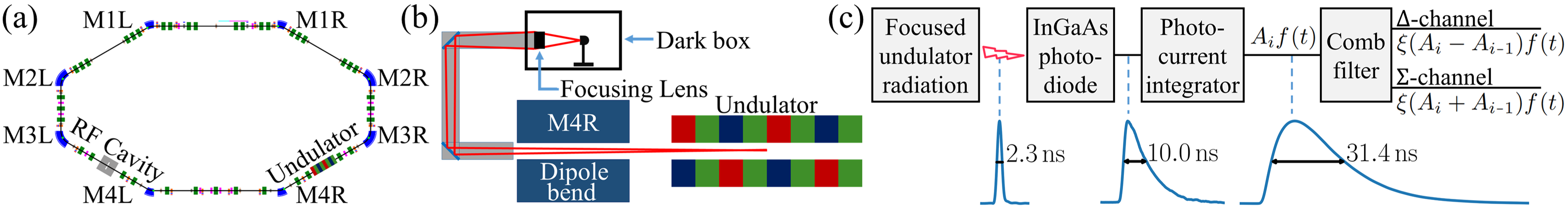
Figure 1: (a) Layout of IOTA, electrons circulate clockwise. (b) Light path from the undulator to the detector (not to scale). (c) Block diagram of the detection circuit, $i$ is the IOTA revolution number. The delay in the comb filter equals exactly one IOTA revolution, $133.3\text{\,}\mathrm{n}\mathrm{s}$. Hence, its $\Delta$-channel provides a signal difference between two consecutive turns.

Most often, noise is encountered in a negative context and is considered something that needs to be minimized. However, there are multiple examples where noise is used as a non-invasive probe into the parameters of a certain system, and even to measure fundamental constants. Examples include the determination of the Boltzmann constant $k_{B}$ by the thermal noise in an electrical conductor [1] and the measurement of the elementary charge $e$ by the shot noise of the electric current in a vacuum tube [2]. In fact, the latter effect is also relevant to accelerators and storage rings, where it is known as Schottky noise [3] due to the finite number of charge carriers in the beam, as described by Schottky [4]. Many beam parameters, such as the momentum spread, the number of particles and even transverse rms emittances, are imprinted into the power spectrum of Schottky noise. It is often used in beam diagnostics [5, 6, 7].

Synchrotron radiation is generated by individual electrons in the beam. Hence, Schottky noise in the beam current must pass on to the synchrotron radiation power in some way. Therefore, one could assume that the synchrotron radiation power noise may carry information about beam parameters as well. This assumption is, in fact, correct. Three decades ago, Ref. [8] reported the results of an experimental study into statistical properties of wiggler radiation in a storage ring. It was noted that the magnitude of turn-to-turn intensity fluctuations depends on the dimensions of the electron bunch. The potential in beam instrumentation was soon realized [9] and a number of papers followed. However, to this day, mostly measurements of a bunch length via these fluctuations were discussed [10, 11, 12]. Only Ref. [13] reported an order-of-magnitude measurement of a transverse emittance. In this Letter, we describe a new fluctuations-based technique for an absolute measurement of a transverse emittance. There are no free parameters in our equations, nor is a calibration required. However, the transverse and longitudinal focusing functions of the storage ring are assumed to be known. This technique is tested at the Integrable Optics Test Accelerator (IOTA) storage ring at Fermilab [14]. For a beam with approximately equal and relatively large transverse rms emittances, the results agree with conventional visible synchrotron light monitors (SLMs) [15]. Then, in a different regime, we measure a much smaller vertical emittance of a flat beam, unresolvable by our SLMs. These emittance measurements agree with estimates, based on the beam lifetime. We also discuss possible further improvements.

Let us assume that we have a detector that can measure the number of detected synchrotron radiation photons $\mathcal{N}$ at each revolution in a storage ring. Then, according to [16, 17, 8, 18], the variance of this number is

$$\mathrm{var}(\mathcal{N})=\langle\big{(}\mathcal{N}-\langle\mathcal{N}\rangle\bigr{)}^{2}\rangle=\langle\mathcal{N}\rangle+\frac{1}{M}\langle\mathcal{N}\rangle^{2},$$ (1)

where the linear term represents the photon shot noise, related to the quantum discrete nature of light. This effect would exist even if there was only one electron, circulating in the ring. Indeed, the electron would radiate photons with a Poisson distribution [19, 20, 21]. The quadratic term in Eq. 1 corresponds to the interference of fields, radiated by different electrons. Changes in relative electron positions and velocities, inside the bunch, result in fluctuations of the radiation power and, consequently, of the number of detected photons. In a storage ring, the effect arises from betatron and synchrotron motion, from radiation induced diffusion, etc. The dependence of $\mathrm{var}(\mathcal{N})$ on the 6D phase-space distribution of the electron bunch is introduced through the parameter $M$, which is conventionally called the number of coherent modes [17, 8, 16]. In addition to bunch parameters, $M$ depends on the specific spectral-angular distribution of the radiation, on the angular aperture, and on the detection efficiency (as a function of wavelength). Previously, we derived an equation for $M$ [22, Eq. (2)] for a Gaussian transverse beam profile and an arbitrary longitudinal bunch density distribution $\rho(z)$ (normalized), assuming an rms bunch length much longer than the radiation wavelength. In this Letter, $M$ is calculated by this equation numerically, using our computer code [23], as a function of transverse emittances $\epsilon_{x}$ and $\epsilon_{y}$, the rms momentum spread $\sigma_{p}$, and the effective bunch length, $\sigma_{z}^{\mathrm{eff}}=1/(2\sqrt{\pi}\int\rho^{2}(z)\differential{z})$, equal to the rms bunch length, $\sigma_{z}$, for a Gaussian distribution.

For illustration purposes, let us assume a Gaussian spectral-angular distribution for the number of detected photons $\mathcal{N}$, namely,

$$\frac{\differential[3]{\mathcal{N}}}{\differential k\differential\theta_{x}\differential\theta_{y}}=C\exp[-\frac{(k-k_{0})^{2}}{2\sigma_{k}^{2}}-\frac{\theta_{x}^{2}}{2\sigma_{\theta_{x}}^{2}}-\frac{\theta_{y}^{2}}{2\sigma_{\theta_{y}}^{2}}\bigr{]},$$ (2)

where $k$ is the magnitude of the wave vector, $\theta_{x}$ and $\theta_{y}$ represent the horizontal and vertical angles of the direction of the radiation in the paraxial approximation, $k_{0}$ refers to the center of the radiation spectrum, $\sigma_{k}$ is the spectral rms width, $\sigma_{\theta_{x}}$ and $\sigma_{\theta_{y}}$ are the angular rms radiation sizes, $C$ is a constant. Then [10, 22]

$$M=\sqrt{1+4\sigma_{k}^{2}\sigma_{z}^{2}}\sqrt{1+4k_{0}^{2}\sigma_{\theta_{x}}^{2}\sigma_{x}^{2}}\sqrt{1+4k_{0}^{2}\sigma_{\theta_{y}}^{2}\sigma_{y}^{2}},$$ (3)

where $\sigma_{x}$, $\sigma_{y}$, $\sigma_{z}$ are the rms sizes (determined by beam emittances) of a Gaussian electron bunch. In addition, it is assumed that the radiation is longitudinally incoherent $k_{0}\sigma_{z}\gg 1$ and that the radiation bandwidth is very narrow $\sigma_{k}\ll 1/(\sigma_{x}\sigma_{\theta_{x}})$, $\sigma_{k}\ll 1/(\sigma_{y}\sigma_{\theta_{y}})$. In general, the distribution parameters $k_{0}$, $\sigma_{k}$, $\sigma_{\theta_{x}}$, $\sigma_{\theta_{y}}$ are determined by both the properties of the emitted synchrotron radiation and by the properties of the detecting system (angular aperture, detection efficiency). In Eq. 3, the beam divergence is neglected and $M$ depends on $\sigma_{x}$ and $\sigma_{y}$, as opposed to a more general result [22, Eq. (2)], where it depends on $\epsilon_{x}$ and $\epsilon_{y}$.

In our experiment, a single electron bunch circulated in IOTA with a revolution period of $133.3\text{\,}\mathrm{n}\mathrm{s}$ and beam energy of $$96.4\text{\,}$\pm$1\text{\,}\mathrm{M}\mathrm{e}\mathrm{V}$$. We studied undulator radiation because the quadratic term in Eq. 1, sensitive to the bunch parameters, is larger for undulators and wigglers than it is for dipole magnets [16]. The undulator parameter is $K_{\mathrm{u}}=$1.0\text{\,}$$ with the number of periods $N_{\mathrm{u}}=$10.5\text{\,}$$ and the period length $\lambda_{\mathrm{u}}=$5.5\text{\,}\mathrm{c}\mathrm{m}$$. The measurements were performed in the vicinity of the fundamental harmonic, $\lambda_{1}=\lambda_{\mathrm{u}}(1+K_{\mathrm{u}}^{2}/2)/(2\gamma^{2})=$1.16\text{\,}\mathrm{\SIUnitSymbolMicro}\mathrm{m}$$, where $\gamma$ is the Lorentz factor. As a photodetector we used an InGaAs PIN photodiode [24], whose quantum efficiency is about $80\text{\,}\mathrm{\char 37\relax}$ around $\lambda_{1}$. The photodiode was installed in a dark box above the M4R dipole magnet, see Figs. 1(a),(b). The light produced in the undulator exited the vacuum chamber through a window at the M4R dipole magnet. It was directed to the box by a system of two mirrors, and focused by a lens (focal distance $F=$150\text{\,}\mathrm{m}\mathrm{m}$$) into a spot, smaller than the photodiode’s sensitive area ($\diameter$1.0\text{\,}\mathrm{m}\mathrm{m}$$). The lens was $3.5\text{\,}\mathrm{m}$ away from the center of the undulator. We numerically calculated the spectral-angular distribution of the undulator radiation by our computer code [25], based on the equations from [26]. Further, we used the manufacturers’ specifications to account for the spectral properties of the optical elements and the photodiode. The resulting spectral width of the radiation was $0.14\text{\,}\mathrm{\SIUnitSymbolMicro}\mathrm{m}$ (FWHM), and the radiation was confined to a cone with a $2\text{\,}\mathrm{m}\mathrm{r}\mathrm{a}\mathrm{d}$ half angle. It could be fully transmitted through the $\diameter$2\text{\,}\mathrm{\text{\textquotedbl}}$$ optical system ($$1\text{\,}\mathrm{\text{\textquotedbl}}$/$3.5\text{\,}\mathrm{m}$=$7.3\text{\,}\mathrm{m}\mathrm{r}\mathrm{a}\mathrm{d}$$). The simulated average number of detected photons per pass, per one electron of the electron bunch was $9.1\text{\times}{10}^{-03}\text{\,}$. The empirical value was $8.8\text{\times}{10}^{-03}\text{\,}$ [22]. There were no free adjustable parameters in this calculation.

Figure 1(c) illustrates our photodetection circuit. First, the radiation pulse is converted into a photocurrent pulse by the photodiode. Then, the photocurrent pulse is integrated by an op-amp-based RC integrator and converted to a voltage signal $A_{i}f(t)$, where $A_{i}$ is the signal amplitude at the $i$th turn and $f(t)$ is the average signal for one turn, normalized so that its maximum value is 1. The number of detected photons (photoelectrons) at the $i$th turn can be obtained as

$$\mathcal{N}_{i}=\chi A_{i},$$ (4)

where $\chi=$2.08\text{\times}{10}^{07}\text{\,}\mathrm{p}\mathrm{h}\mathrm{o}\mathrm{t}\mathrm{o}\mathrm{e}\mathrm{l}\mathrm{e}\mathrm{c}\mathrm{t}\mathrm{r}\mathrm{o}\mathrm{n}\mathrm{s}\mathrm{/}\mathrm{V}$$, with a $5\text{\,}\mathrm{\char 37\relax}$ uncertainty, as per the characteristics of our integrator and the photodiode [22]. The op-amp was capable of driving the 50-$\Omega$ input load of a fast digitizing scope, located $\approx$100\text{\,}\mathrm{m}$$ away. In our measurements, $A_{i}\in[0,1.2]$\text{\,}\mathrm{V}$$.

The expected relative fluctuation of $A_{i}$ was ${10}^{-4}{10}^{-3}\text{\,}$ (rms), which is considerably lower than the digitization resolution of our 8-bit broad-band oscilloscope. To overcome this problem, we employed a passive comb (notch) filter [27], see Fig. 1(c). In this filter, the input signal first passes through a two-way splitter. One arm is delayed relative to the other by exactly one IOTA revolution. Then, the difference and the sum of the two signals are produced in the output $\Delta$- and $\Sigma$-channels. For an ideal comb filter,

$$\Delta_{i}(t)=\xi(A_{i}-A_{i\shortminus 1})f(t),$$ (5)

$$\Sigma_{i}(t)=\xi(A_{i}+A_{i\shortminus 1})f(t).$$ (6)

In our filter, $\xi=$0.31\text{\,}$$, which was measured by comparing input and output pulses. Now, since the offset was removed (Eq. 5), we were able to directly observe the sub-$\text{\,}\mathrm{m}\mathrm{V}$ turn-to-turn fluctuations in the $\Delta$-channel and the oscilloscope operated in the appropriate scale setting with negligible digitization noise.

For each measurement, we recorded $1.5\text{\,}\mathrm{m}\mathrm{s}$-long waveforms (about $11\,250\text{\,}$ IOTA revolutions) of $\Delta$- and $\Sigma$-channels with the oscilloscope at $20\text{\,}\mathrm{G}\mathrm{S}\mathrm{a}\mathrm{/}\mathrm{s}$. The beam current decay was negligible during the acquisition time. The photoelectron count variance $\mathrm{var}(\mathcal{N})$ and the photoelectron count mean $\langle\mathcal{N}\rangle$ were obtained from the $11\,250\text{\,}$ collected amplitudes, $\Delta_{i}(t_{\mathrm{peak}})$ and $\Sigma_{i}(t_{\mathrm{peak}})$, as

$$\mathrm{var}(\mathcal{N})=\chi^{2}\mathrm{var}(A)=\frac{\chi^{2}\mathrm{var}(\Delta(t_{\mathrm{peak}}))}{2\xi^{2}},$$ (7)

$$\langle\mathcal{N}\rangle=\chi\langle A\rangle=\chi\frac{\langle\Sigma(t_{\mathrm{peak}})\rangle}{2\xi},$$ (8)

where $t_{\mathrm{peak}}$ is the time within each turn corresponding to the peak of the signal, $f(t_{\mathrm{peak}})=1$. These formulas follow from Eqs. 4, 5 and 6. There was a small cross-talk ($<$1\text{\,}\mathrm{\char 37\relax}$$) between the output channels of the comb filter. However, its effect is negligible in Eqs. 7 and 8. Also, there was some instrumental noise contribution to $\mathrm{var}(\Delta(t_{\mathrm{peak}}))$. Its contribution to $\mathrm{var}(\mathcal{N})$ was $2.0\text{\times}{10}^{08}\text{\,}$, as measured at zero beam current. Primary sources of this noise were the integrator’s op-amp and the oscilloscope’s pre-amp. In [22], we showed that this noise level was independent of $\langle\mathcal{N}\rangle$ via measurements with an independent test light source. Therefore, it can be simply subtracted. Reference [22] also describes the details of the photocurrent integrator and the comb filter.

The number of coherent modes $M$ and, hence, the fluctuations $\mathrm{var}(\mathcal{N})$ depend on the following bunch parameters: $\epsilon_{x}$, $\epsilon_{y}$ (or mode emittances $\epsilon_{1}$, $\epsilon_{2}$), $\sigma_{p}$, $\sigma_{z}^{\mathrm{eff}}$. When only one of them is unknown and $\mathrm{var}(\mathcal{N})$ is known (or measured), we can numerically solve Eq. 1, using our general formula for $M$ [22, Eq. (2)], to find the unknown bunch parameter. Below we consider two such situations.

In the first case, we consider a strongly coupled [28, 29] transverse focusing optics in IOTA, which was specifically designed to keep the two mode emittances equal $\epsilon_{1}=\epsilon_{2}=\epsilon$. This was empirically confirmed to be true with a few percent precision. We will call this setup “round beam”. The longitudinal bunch profile was measured by a high-bandwidth wall-current monitor [30] to determine $\sigma_{z}^{\mathrm{eff}}$ and estimate $\sigma_{p}$. The fluctuations $\mathrm{var}(\mathcal{N})$, measured using Eq. 7, are shown in Fig. 2(a), with a statistical error of $2.7\text{\times}{10}^{06}\text{\,}$ (at all beam currents), which was determined with an independent test light source [22]. Hence, the only unknown parameter in Eq. 1 is $\epsilon$. The numerical solution of Eq. 1 with $M$ from [22, Eq. (2)] was performed on the Midway2 cluster at the University of Chicago Research Computing Center. The results for $\epsilon$ are shown in Fig. 2(c) (red points). The error bars correspond to the statistical error of the fluctuations measurement. Apart from this statistical error there is also a systematic error due to the $1\text{\,}\mathrm{M}\mathrm{e}\mathrm{V}$ uncertainty on the beam energy (from $10\text{\,}\mathrm{n}\mathrm{m}$ at lower beam currents to $14\text{\,}\mathrm{n}\mathrm{m}$ at higher currents).

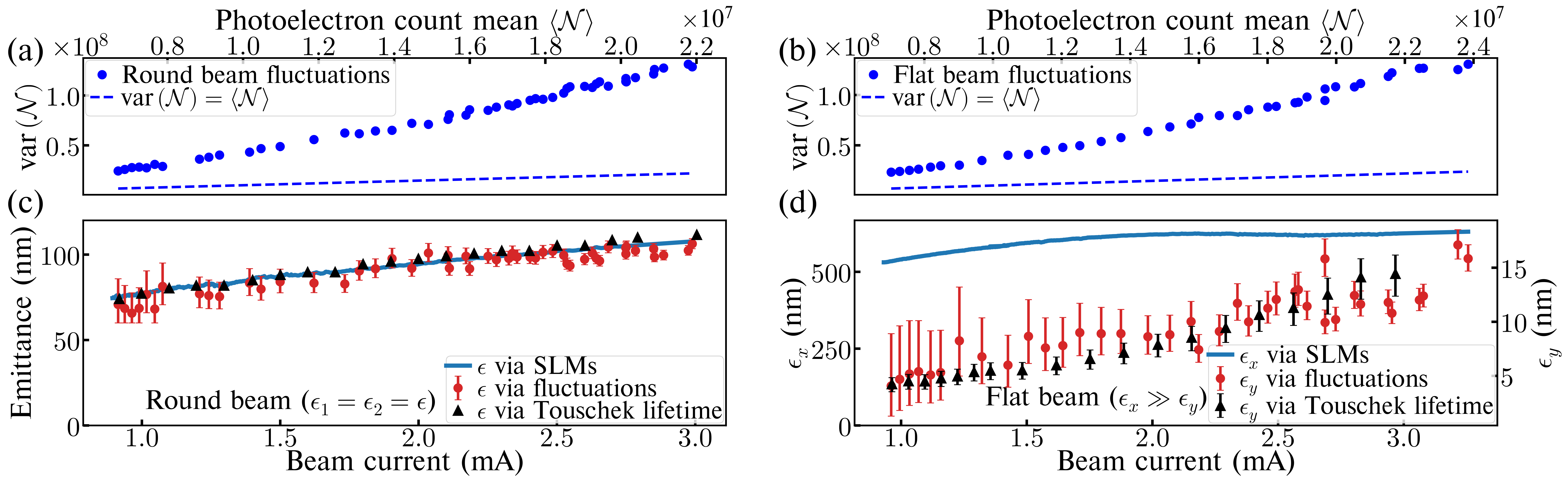
Figure 2: Panels (a) and (b) show the measured fluctuations for the round and flat beams, respectively. The statistical error of each point is $2.7\text{\times}{10}^{06}\text{\,}$ (not shown). (c) The round-beam mode emittance $\epsilon$, determined via SLMs, via undulator radiation fluctuations, and via Touschek lifetime, assuming the effective momentum acceptance $2.0\text{\times}{10}^{-03}\text{\,}$. (d) The flat-beam horizontal emittance measurement via SLMs (left scale), the vertical emittance measurement via fluctuations and via Touschek lifetime (right scale). The SLMs had a monitor-to-monitor spread of $\pm$8\text{\,}\mathrm{n}\mathrm{m}$$ (round beam) and $\pm$50\text{\,}\mathrm{n}\mathrm{m}$$ (horizontal emittance of flat beam); these error bars are not shown. All emittances are rms, unnormalized.

In IOTA, transverse beam sizes are monitored by seven SLMs, at M1L–M4L and at M1R–M3R, see Fig. 1(a). Beam emittances can be determined from the measured sizes using the design Twiss functions. Such measurements for $\epsilon$ of the round beam [blue line in Fig. 2(c)] agree with the fluctuations-based $\epsilon$ within the uncertainties. The smallest reliably resolvable emittance by the SLMs in our experiment configuration was $\approx$20\text{\,}\mathrm{n}\mathrm{m}$$. The measured round-beam emittance $\epsilon$ is $75100\text{\,}\mathrm{n}\mathrm{m}$ (rms, unnormalized), primarily due to intrabeam scattering [31, 32]. The expected zero-current value is $\epsilon\approx$12\text{\,}\mathrm{n}\mathrm{m}$$.

In the second case, we consider uncoupled focusing, with the vertical emittance much smaller than the horizontal one. We will call this configuration “flat beam”. The horizontal emittance $\epsilon_{x}$ of the flat beam can still be reliably measured by the SLMs; $\sigma_{z}^{\mathrm{eff}}$ and $\sigma_{p}$ can still be measured by the wall-current monitor. However, the seven SLMs provided very inconsistent estimates for the much smaller $\epsilon_{y}$ — the max-to-min variation for different SLMs reached a factor of eight. We believe this happened because the beam images were close to the resolution limit, set by a combination of factors, such as the diffraction limit, the point spread function of the cameras, chromatic aberrations, the effective radiator size of the dipole magnet radiation ($\approx$20\text{\,}\mathrm{\SIUnitSymbolMicro}\mathrm{m}$$), and the camera pixel size ($\approx$10\text{\,}\mathrm{\SIUnitSymbolMicro}\mathrm{m}$$ in terms of beam size). Therefore, the monitor-to-monitor emittance variation primarily came from the Twiss beta-function variation ($\beta_{y}^{(\mathrm{max})}/\beta_{y}^{(\mathrm{min})}\approx 12$). Although the resolution of the SLMs may be improved in the future [22], at present, $\epsilon_{y}$ of the flat beam is unresolvable by the SLMs, and, therefore, is truly unknown. However, the measured fluctuations for the flat beam, shown in Fig. 2(b), were of the same order as for the round beam, with the same statistical error. Hence, we were able to reconstruct $\epsilon_{y}$ in the same way as $\epsilon$ in Fig. 2(c). The results are shown in Fig. 2(d) (red points, right vertical scale) along with the SLMs data for $\epsilon_{x}$ (blue line, left vertical scale). In addition to the statistical error of $\epsilon_{y}$, shown in Fig. 2(d), there was also a systematic error due to the $1\text{\,}\mathrm{M}\mathrm{e}\mathrm{V}$ uncertainty on the beam energy (from $2.5\text{\,}\mathrm{n}\mathrm{m}$ at lower currents to $5\text{\,}\mathrm{n}\mathrm{m}$ at higher currents), and a systematic error due to the $50\text{\,}\mathrm{n}\mathrm{m}$ uncertainty on $\epsilon_{x}$ (from $1.3\text{\,}\mathrm{n}\mathrm{m}$ at lower currents to $2.4\text{\,}\mathrm{n}\mathrm{m}$ at higher currents). The measured vertical emittance is $515\text{\,}\mathrm{n}\mathrm{m}$, most likely due to a nonzero residual transverse coupling. The expected zero-current flat-beam emittances were $\epsilon_{x}\approx$50\text{\,}\mathrm{n}\mathrm{m}$$, $\epsilon_{y}\gtrsim$0.33\text{\,}\mathrm{p}\mathrm{m}$$ (set by the quantum excitation in a perfectly uncoupled ring).

The vertical emittance $\epsilon_{y}$ of the flat beam in IOTA could also be estimated from the measured beam lifetime $\left|I/(\derivative*{I}{t})\right|$, assuming that it is determined solely by Touschek scattering [33], which is a good approximation at beam currents $I\gtrsim$0.5\text{\,}\mathrm{m}\mathrm{A}$$ [29]. In storage rings, the Touschek lifetime is determined by the effective momentum acceptance $\delta_{\mathrm{acc}}^{(\mathrm{eff})}$ [34], which is smaller than or equal to the rf bucket half-height, $\delta_{\mathrm{rf}}=$2.8\text{\times}{10}^{-03}\text{\,}$$ in IOTA. We measured the IOTA beam lifetime ($5501000\text{\,}\mathrm{s}$) for both round and flat beams as a function of beam current. Using the known round-beam emittance and the bunch length, we arrived at the following estimate for IOTA, $\delta_{\mathrm{acc}}^{(\mathrm{eff})}=$2.0\text{\times}{10}^{-03}\text{\,}$$, by comparing the calculated [35, 36] Touschek lifetime and the measured beam lifetime (for details see Appendix D of [22]). The black triangles in Fig. 2(c) illustrate the emittance of the round beam $\epsilon$, determined from the measured beam lifetime using the Touschek lifetime calculation with $\delta_{\mathrm{acc}}^{(\mathrm{eff})}=$2.0\text{\times}{10}^{-03}\text{\,}$$. Then, we used this value of $\delta_{\mathrm{acc}}^{(\mathrm{eff})}$ and the values of $\epsilon_{x}$, measured by the SLMs, to estimate the vertical emittance $\epsilon_{y}$ of the flat beam via the Touschek lifetime. The results are shown in Fig. 2(d) (black triangles). The error bars correspond to the $\pm$50\text{\,}\mathrm{n}\mathrm{m}$$ uncertainty on $\epsilon_{x}$.

During our measurements, the rms and the effective bunch lengths $\sigma_{z}$, $\sigma_{z}^{\mathrm{eff}}$ were $2631\text{\,}\mathrm{c}\mathrm{m}$ and $2430\text{\,}\mathrm{c}\mathrm{m}$, respectively, primarily due to intrabeam scattering. They were different because the longitudinal bunch shape was not exactly Gaussian due to beam interaction with its environment [37]. The relative rms momentum spread was $\sigma_{p}\approx$9.1\text{\times}{10}^{-06}\text{\,}$\times\sigma_{z}[\mathrm{cm}]$, based on the rf cavity and ring parameters. The expected zero-current values are $\sigma_{z}=\sigma_{z}^{\mathrm{eff}}=$9\text{\,}\mathrm{c}\mathrm{m}$$, $\sigma_{p}=$8.3\text{\times}{10}^{-05}\text{\,}$$. The uncoupled case Twiss beta-functions in the undulator were $\beta_{x}=$204\text{\,}\mathrm{c}\mathrm{m}$$, $\beta_{y}=$98\text{\,}\mathrm{c}\mathrm{m}$$, for more details see [22].

Other emittance monitors (wire scanners, Compton-scattering monitors [38, 39]) could provide better resolution in IOTA. However, if a bright synchrotron light source is available, our fluctuations-based monitor may be a good inexpensive non-invasive alternative. There are two requirements for the technique to work: (A) the fluctuations should not be dominated by the Poisson noise, so that $M$ can be reliably deduced from $\mathrm{var}(\mathcal{N})$, and (B) $M$ has to be sensitive to $\epsilon_{x}$, $\epsilon_{y}$. Let us consider the $h$th harmonic of undulator radiation in the approximation of Eqs. 2 and 3 with a narrow Gaussian filter $\sigma_{k}\ll k_{0}/(hN_{\mathrm{u}})$ and $k_{0}=2\pi h/\lambda_{1}$. By integrating Eq. 2 we obtain $\langle\mathcal{N}\rangle=C(2\pi)^{3/2}\sigma_{\theta_{x}}\sigma_{\theta_{y}}\sigma_{k}$, where $C$ is the peak on-axis photon flux, $C=\alpha N_{\mathrm{u}}^{2}\gamma^{2}F_{h}(K_{\mathrm{u}})n_{e}/k_{0}$ [26, p. 68], $\alpha$ is the fine-structure constant, $n_{e}$ is the number of electrons per bunch, and the function $F_{h}(K_{\mathrm{u}})$, defined in [26, p. 69], is typically about $0.20.4\text{\,}$. If we approximate Eq. 3 by $M\approx 8\,k_{0}^{2}\,\sigma_{k}\sigma_{\theta_{x}}\sigma_{\theta_{y}}\sigma_{x}\sigma_{y}\sigma_{z}$, the requirement (A) becomes [see Eq. 1]

$$\frac{\langle\mathcal{N}\rangle}{M}=\alpha\left(\frac{\pi}{2}\right)^{\frac{3}{2}}F_{h}(K_{\mathrm{u}})\frac{\gamma^{2}N_{\mathrm{u}}^{2}n_{e}}{\sigma_{x}\sigma_{y}\sigma_{z}k_{0}^{3}}\gtrsim 1.$$ (9)

In the model of Eq. 3, the requirement (B) becomes $\sigma_{x}\gtrsim 1/(2k_{0}\sigma_{\theta_{x}})$, $\sigma_{y}\gtrsim 1/(2k_{0}\sigma_{\theta_{y}})$. Notably, one can intentionally make $M$ insensitive to $\sigma_{x}$ (or $\sigma_{y}$), and, thus, enable an independent measurement of $\sigma_{y}$ (or $\sigma_{x}$). For example, by using a vertical slit, which can be approximated by a very small $\sigma_{\theta_{x}}\ll 1/(2k_{0}\sigma_{x})$, one can deduce $\sigma_{y}$ from a measured $M$ without the knowledge of $\sigma_{x}$. Also, radiation masks can be applied to analyze fluctuations in various portions of the angular distribution of the radiation, which adds flexibility to this method. Assuming no angular restrictions, $\sigma_{\theta_{x}},\sigma_{\theta_{y}}\approx\sqrt{\lambda_{0}/(2L_{\mathrm{u}})}$ [17, Eq. (2.57)], and the requirement (B) becomes

$$\sigma_{x},\sigma_{y}\gtrsim\sqrt{2L_{\mathrm{u}}\lambda_{0}}/(4\pi),$$ (10)

where $\lambda_{0}=2\pi/k_{0}$, $L_{\mathrm{u}}$ is the undulator length. In IOTA, this corresponds to $\sigma_{x},\sigma_{y}\gtrsim$50\text{\,}\mathrm{\SIUnitSymbolMicro}\mathrm{m}$$, or $\epsilon_{x}\gtrsim$1.0\text{\,}\mathrm{n}\mathrm{m}$$, $\epsilon_{y}\gtrsim$2.2\text{\,}\mathrm{n}\mathrm{m}$$; and $\langle\mathcal{N}\rangle/M\in[2.3,5.0]$ (as per measurements).

Equation (10) shows that the resolution limit improves with a shorter wavelength. Therefore, this technique may be particularly beneficial for existing state-of-the-art and next generation low-emittance high-brightness ultraviolet and x-ray synchrotron light sources. Consider the Advanced Photon Source Upgrade (APS-U) with a round beam configuration for example. The beam energy is $6\text{\,}\mathrm{G}\mathrm{e}\mathrm{V}$, $n_{e}=$9.6\text{\times}{10}^{10}\text{\,}$$, $\sigma_{z}=$3.1\text{\,}\mathrm{c}\mathrm{m}$$, $\epsilon_{x}=$31.9\text{\,}\mathrm{p}\mathrm{m}$$, $\epsilon_{y}=$31.7\text{\,}\mathrm{p}\mathrm{m}$$, $\sigma_{x}=$12.9\text{\,}\mathrm{\SIUnitSymbolMicro}\mathrm{m}$$, $\sigma_{y}=$8.7\text{\,}\mathrm{\SIUnitSymbolMicro}\mathrm{m}$$, $\sigma_{x^{\prime}}=$2.5\text{\,}\mathrm{\SIUnitSymbolMicro}\mathrm{r}\mathrm{a}\mathrm{d}$$, $\sigma_{y^{\prime}}=$3.6\text{\,}\mathrm{\SIUnitSymbolMicro}\mathrm{r}\mathrm{a}\mathrm{d}$$ [40]. Let us use the fundamental harmonic $\lambda_{1}=$4.1\text{\,}\mathrm{\SIUnitSymbolAngstrom}$$ of the undulator with $\lambda_{\mathrm{u}}=$28\text{\,}\mathrm{m}\mathrm{m}$$, $K_{\mathrm{u}}=$2.459\text{\,}$$, and $L_{\mathrm{u}}=$2.1\text{\,}\mathrm{m}$$. Equation (9) yields $\langle\mathcal{N}\rangle/M=$19\text{\,}$$, and Eq. 10 becomes $\sigma_{x},\sigma_{y}\gtrsim$3.3\text{\,}\mathrm{\SIUnitSymbolMicro}\mathrm{m}$$. Thus, both requirements (A) and (B) are satisfied. These estimates were confirmed by [22, Eqs. (2–8)].