Carbonate-Silicate Cycle Predictions of Earth-like Planetary Climates and Testing the Habitable Zone Concept

Abstract

In the conventional habitable zone (HZ) concept, a CO₂-H₂O greenhouse maintains surface liquid water. Through the water-mediated carbonate-silicate weathering cycle, atmospheric CO₂ partial pressure (pCO₂) responds to changes in surface temperature, stabilizing the climate over geologic timescales. We show that this weathering feedback ought to produce a log-linear relationship between pCO₂ and incident flux on Earth-like planets in the HZ. However, this trend has scatter because geophysical and physicochemical parameters can vary, such as land area for weathering and CO₂ outgassing fluxes. Using a coupled climate and carbonate-silicate weathering model, we quantify the likely scatter in pCO₂ with orbital distance throughout the HZ. From this dispersion, we predict a two-dimensional relationship between incident flux and pCO₂ in the HZ and show that it could be detected from at least 83 ($2{\sigma}$) Earth-like exoplanet observations. If fewer Earth-like exoplanets are observed, testing the HZ hypothesis from this relationship could be difficult.

1 Introduction

Newton first alluded to the concept of a stellar habitable zone (HZ) in his 1687 Principia[1] by noting that Earth’s liquid water would vaporize or freeze at the orbits of Mercury and Saturn, respectively[2]. Later, Whewell noted that “the Earth’s orbit is in the temperate zone of the Solar System”[3]. Since then, the definition of the stellar HZ has been refined, reaching its modern incarnation based on climate models [4, 5].

Current HZ calculations [6] find that around a Sun-like star, an Earth-like planet could remain habitable between 0.97 and 1.70 AU. The inner edge of the HZ is set by loss of surface water and the outer edge is set by the maximum greenhouse of a CO₂ atmosphere where extensive CO₂ condensation and increased Rayleigh scattering prevent any further greenhouse warming from CO₂ [7, 6]. This definition of the HZ only considers H₂O and CO₂ as greenhouse gases, so Earth-like planets warmed by other greenhouse gases (e.g. H₂ or CH₄) could remain habitable at bigger orbital distances [8, 9, 5]. However, CH₄-rich atmospheres in the HZ may not be possible without life to generate substantial CH₄ [10, 11]. In addition, more complex climate models have shown the HZ might extend to smaller orbital distances, perhaps interior to Venus’ orbit, with appropriate planetary conditions [12, 13, 14, 15].

Residing within the HZ does not guarantee habitable surface conditions. Crucially, greenhouse gas abundances (and planetary albedo) must conspire to produce clement surface conditions. For example, by most estimates, Mars resides within the Sun’s HZ but is not habitable because there is insufficient greenhouse warming from CO₂, in part because of the lack of volcanic outgassing of CO₂. Thus, considering the planetary processes that control atmospheric CO₂ abundances on Earth-like planets in the HZ is necessary to constrain planetary habitability.

The prevailing hypothesis is that CO₂ levels are controlled by a weathering thermostat [16]. This can explain why Earth has maintained a clement surface throughout its history despite the ${\sim}$30% brightening of the Sun over the past ${\sim}$4.5 Gyr [17, 18, 19, 20, 21]. The changing luminosity of the Sun with time is similar to moving a planet through the HZ, and so the same CO₂ weathering process responsible for maintaining habitability on the Earth through time, the carbonate-silicate weathering cycle, may similarly stabilize planetary climates within the HZ.

In the carbonate-silicate cycle, atmospheric CO₂ dissolves in water and weathers silicates on both the continents and seafloor, which releases cations and anions [22, 16, 23, 24, 25, 26, 27]. On the continents, the weathering products, including dissolved SiO₂, HCO${}_{3}^{-}$, and Ca⁺⁺, wash into the oceans where the HCO${}_{3}^{-}$ combine with cations like Ca⁺⁺ to create CaCO₃, which precipitates out of solution. The net process converts atmospheric CO₂ into marine carbonate minerals (i.e., CaCO₃). Also, seafloor weathering occurs when seawater releases Ca⁺⁺ ions from the seafloor basalt and CaCO₃ precipitates in pores and veins. Subsequently, the carbonates within sediments and altered seafloor can be subducted.

Carbon returns to the atmosphere from outgassing. If CO₂ outgassing increases above the steady-state outgassing rate, a planet’s surface temperature rises. This leads to increased rainfall and continental weathering as well as potentially warmer deep-sea temperatures and more seafloor weathering [21, 24, 28]. Increased weathering draws down atmospheric CO₂ and stabilizes the climate over ${\sim}10^{6}$-year timescales on habitable, Earth-like planets [29].

One- and three-dimensional climate calculations of HZ limits [4, 6, 14] assume that a carbonate-silicate weathering cycle is functioning but do not explicitly include it. The assumed presence of the carbonate-silicate cycle would predict that atmospheric CO₂ of Earth-like planets increases with orbital distance in the HZ [4, 6, 29]. In particular, future telescopic observations, e.g. NASA’s Habitable Exoplanet Imaging Mission (HabEx)[30] and Large Ultraviolet Optical Infrared Surveyor (LUVOIR)[31], could search for the CO₂ trend to test the HZ hypothesis [32, 33, 34]. Previous studies [35, 29] have suggested the carbonate-silicate weathering cycle could alter predictions of pCO₂ in the HZ, but it is important to know the exact relationship we are looking for. Also, while an increase of pCO₂ with orbital distance in the HZ may be true if all Earth-like exoplanets have the exact same properties as the modern Earth, the trend becomes less certain if HZ planetary characteristics deviate from those of the modern Earth. There could be considerable variability in atmospheric CO₂ throughout the HZ, perhaps even enough to obscure a monotonic trend with orbital distance.

Here, we show that uncertain physicochemical and geophysical parameters in the carbonate-silicate weathering cycle [26] cause scatter in pCO₂ with orbital distance. We then demonstrate that future telescopes must observe at least 83 ($2\sigma$) HZ planetary atmospheres to confidently detect our predicted relationship between atmospheric CO₂ and orbital distance, and confirm the HZ hypothesis.

2 Results

2.1 Stable pCO₂ abundances from our numerical model

Parameter	Parameter Description	Range	Scaling	Units
$F_{\textrm{out}}^{\textrm{mod}}$	Modern CO2 outgassing flux	6-10		Tmol C yr-1
$n$	Carbonate precipitation coefficient	1-2.5	$\propto\left[\textrm{CO}^{2-}_{3}\right]^{\textrm{n}}$
$x$	Modern seafloor dissolution relative to precipitation	0.5-1.5	$\propto xF_{\textrm{out}}^{\textrm{mod}}$
$T_{\textrm{e}}$	E-folding temperature factor for continental weathering	10-40		K
$\alpha$	Power law exponent for CO2 dependence of continental silicate weathering	0.1-0.5	$\propto\left(\textrm{pCO}_{2}\right)^{\alpha}$
$\xi$	Power law exponent for CO2 dependence of continental carbonate weathering	0.1-0.5	$\propto\left(\textrm{pCO}_{2}\right)^{\xi}$
$f_{\textrm{land}}$	Land fraction compared to modern Earth	0-1
$S_{\textrm{thick}}$	Ocean sediment thickness relative to modern Earth	0.2-1
$F_{\textrm{carb}}^{\textrm{mod}}$	Modern continental carbonate weathering	7-14		Tmol C yr-1
$f_{\textrm{bio}}$	Biological weathering compared to modern Earth	0-1
$a_{\textrm{grad}}$	Surface to deep ocean temperature gradient scaling	0.8-1.4	$\propto a_{\textrm{grad}}T_{\textrm{s}}$
$\gamma$	Power law exponent for pH dependence of seafloor dissolution	0-0.5	$\propto\left(\left[\textrm{H}^{+}\right]\right)^{\gamma}$
$\beta$	Power law exponent for seafloor spreading rate	0-0.2	$\propto Q^{\beta}$
$m$	Exponent for outgassing dependence on crustal production	1-2	$\propto Q^{\textrm{m}}$
$E_{\textrm{bas}}$	Seafloor dissolution activation energy	60-100		kJ mol-1
$n_{\textrm{out}}$	Exponent for internal heat with time	0-0.73	see eq. 10
$\tau$	Planet age (see eq. 10)*	0-10		Gyr
$S$	Incident flux relative to modern Earth*	0.35-1.05

Table 1: Parameter ranges for our numerical model. Parameters are dimensionless unless otherwise described. The fourth column shows how scaling parameters impact the model, where $T_{\textrm{s}}$ is the surface temperature in K and $Q$ is the internal heat of the planet relative to the modern Earth (see equation 10 for $Q$). Unless otherwise noted, each parameter range is justified in the original model derivation for the Earth through time[21]. *The justification for this parameter is given in the Methods, subsection Numerical carbonate-silicate cycle modeling.

We use a coupled climate and carbonate-silicate weathering model (see Methods, subsection Numerical carbonate-silicate cycle modeling) to explore pCO₂ on Earth-like planets in the HZ. The model considers numerous planetary properties, listed in Table 1, and their effect on the carbonate-silicate weathering cycle to calculate a planet’s steady-state pCO₂ and surface temperature. If the globally averaged, steady-state surface temperature is below 248 K, we assume the planet is completely frozen and uninhabitable at the surface, as shown by three-dimensional climate models [36]. Similarly, we assume planets are uninhabitable beyond 355 K, above which surface water would be rapidly lost to space [37] (see Methods, subsection Numerical carbonate-silicate cycle modeling for additional details on these assumed temperature constraints).

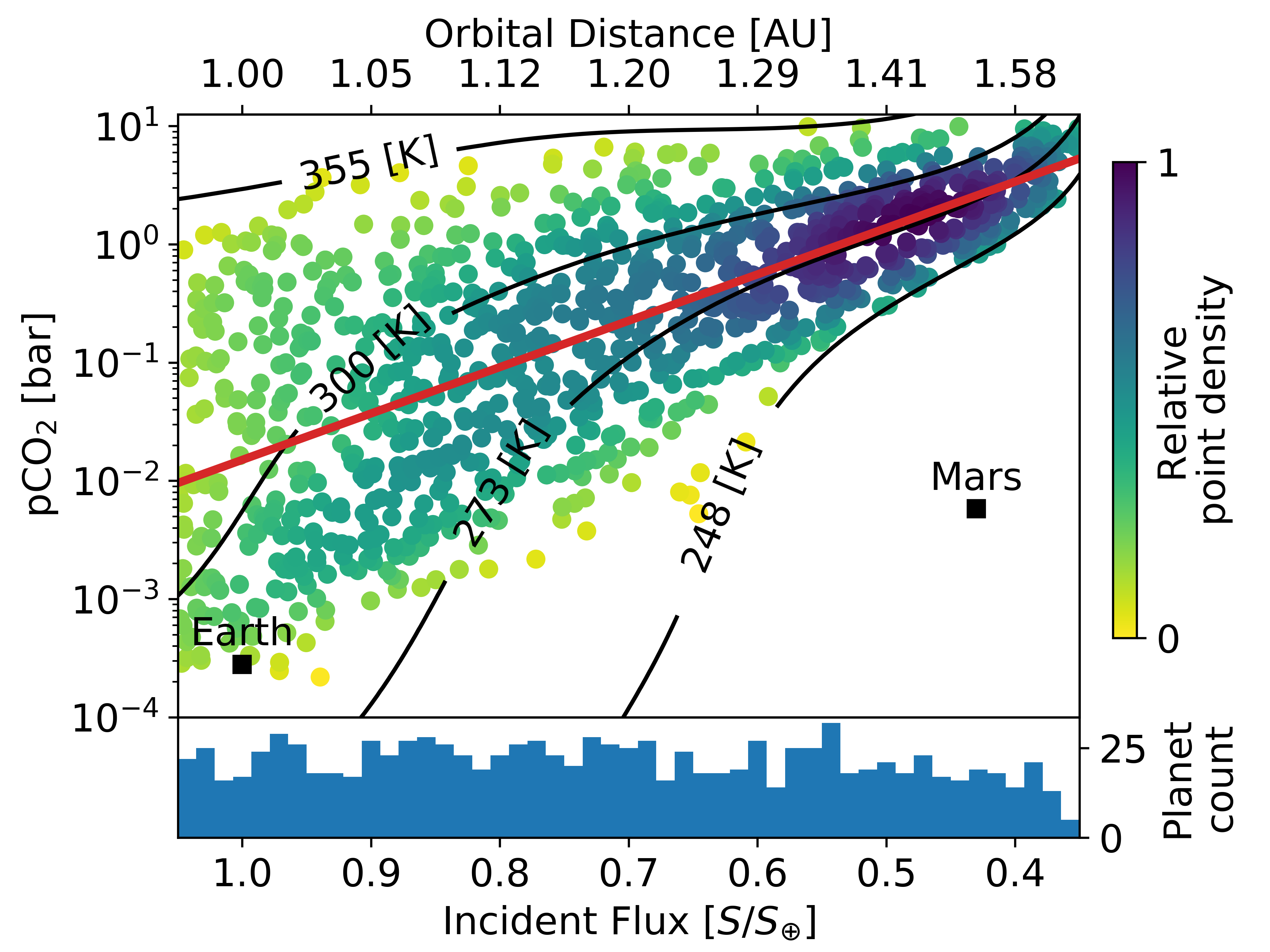
Figure 1: The expected distribution of stable, Earth-like exoplanet climates from our habitable zone weathering model. The horizontal axis shows incident flux, $S$, normalized to the solar constant ($S_{\oplus}$) and the corresponding orbital distance in Astronomical Units (AU) above the plot. The vertical axis shows the atmospheric CO₂ partial pressure (pCO₂) in bar. Each point represents a climate in steady state. The black labeled contours show the mean global surface temperature for the given pCO₂ and incident flux. The white region below the 248 K contour is where our model assumption of a liquid ocean is no longer plausible so no planets are shown in that region. Above the 355 K contour Earth-like planets are too hot to retain their liquid oceans for billions of years. Similar to the frozen planets, such hot planets are not considered habitable. Modern Earth and Mars are shown by black squares. The blue histogram at the bottom of the figure shows the number of stable planets in each incident flux bin. The color of each simulated planet shows the relative point density in the plot at that location. The color was calculated using a kernel-density estimate with Gaussian kernels and rescaled from 0 to 1. A color value of 0 represents the lowest relative point density, 1 the highest. The log-linear line of best fit between pCO₂ and $S$ is shown in red. The slope of the red, best fit line is 3.92$\pm$0.24 (95%) with units -$\log_{10}$(pCO₂ [bar])/[$S/S_{\oplus}$]. Our model predicts that atmospheric CO₂ should increase with orbital distance in the HZ.

We randomly generated 1050 habitable, stable, Earth-like exoplanet climates using uniform distributions of the model parameters in Table 1. A total of 1200 random, initial parameter combinations were considered but we eliminated those that resulted in planets that froze completely or were too hot to retain their surface oceans. As colored dots, Figure 1 shows habitable, steady-state solutions.

Our model predicts that atmospheric CO₂ abundances should broadly increase and narrow in their spread with orbital distance in the HZ (Figure 1), consistent with other models of CO₂ in the HZ [29, 38]. As justified next in Section 2.2, the scatter is about a nominal linear trend between incident flux, $S$, and log(pCO₂), which is different from a non-linear trend in models that assume a constant surface temperature in the HZ from negative feedbacks [32, 34] but do not actually model the carbonate-silicate feedbacks. If future missions are to test the HZ concept by searching for a trend between incident flux, $S$, and pCO₂ [32, 33, 34], they could search for the fundamental $S$-pCO₂ relationship shown in Figure 1.

Below, we show that a log-linear relationship between pCO₂ and $S$ may be the default in the HZ if Earth-like carbonate-silicate weathering is ubiquitous on habitable planets. In fact, the trend is elucidated by combining climate theory with carbonate-silicate cycle theory in what follows.

2.2 Habitable zone climate theory revisited

Figure 2: The relationship between incident flux and atmospheric CO₂ for Earth-like planets regulated by a carbonate-silicate weathering cycle. The horizontal axis shows incident flux, $S$, normalized to the solar constant ($S_{\oplus}$) and the corresponding orbital distance in Astronomical Units (AU) above the plot. The vertical axis shows the atmospheric CO₂ partial pressure (pCO₂) in bar. The dotted blue curve labelled 289 K shows the pCO₂ value required to maintain a 289 K surface temperature for the given incident flux, $S$. The conventional assumption of CO₂ in the HZ stipulates that pCO₂ will adjust to maintain a temperate or even constant surface temperature. Under this assumption, moving the modern Earth (labelled black square) outward in the HZ would have the planet approximately follow the dotted blue 289 K contour. The colored points and gray curves show the modern Earth moving outward in the HZ with a functioning carbonate-silicate weathering cycle, calculated from equation 6. We consider two temperature and pCO₂ dependencies for continental weathering in this plot. The strong temperature dependence contour (labelled Strong T-dep.), uses a temperature and pCO₂-dependent weathering factor of $\alpha T_{\textrm{e}}=2.3$, which implies a strong temperature feedback on continental weathering compared to the pCO₂ feedback (see equation 7). The moderate temperature dependence contour (labelled Moderate T-dep.), uses a temperature and pCO₂-dependent weathering factor of $\alpha T_{\textrm{e}}=7.5$. These two values for $\alpha T_{\textrm{e}}$ result in two different paths the Earth can take as it moves outward in the HZ. The planet color shows the mean surface temperature. Log-linear fits to the colored points of the Strong T-dep. and Moderate T-dep. contours have r² values of 0.959 and 0.999, respectively. Thus, even for a strong temperature dependence of continental weathering, our coupled climate and weathering model predicts an approximately log-linear relationship between incident flux and pCO₂ on Earth-like planets in the HZ.

A conventional assumption is that the carbonate-silicate weathering cycle will approximately maintain a stable, temperate surface temperature for an Earth-like planet moved about in the HZ [39, 7, 6] or even a constant temperature [32, 34]. Thus, if we moved the modern Earth outward in the HZ, the smaller incident flux would initially cause the planet to cool. The cooler temperature would lower the CO₂ weathering rate causing CO₂ to accumulate in the atmosphere until the temperature returned to its nominal value of 289 K. Figure 2 shows this scenario with the dotted blue 289 K contour, which gives the pCO₂ value required to maintain a 289 K surface temperature for the modern Earth as it moves about the HZ. The line was calculated from a radiative-convective climate model described in the Methods below, subsection Habitable zone 1D climate model (see equation 8).

The constant, 289 K surface temperature contour in Figure 2 is a non-linear relationship between incident flux, $S$, and log(pCO₂) but it does not consider the temperature and pCO₂ feedbacks inherent to the carbonate-silicate weathering cycle. We demonstrate that if these feedbacks are taken into account, surface temperature declines with orbital distance, as mentioned in previous work [29], and the relationship between $S$ and log(pCO₂) is actually approximately linear for Earth-like planets in the HZ.

If Bond albedo is fixed, the surface temperature, $T_{\textrm{s}}$, for an Earth-like planet in steady-state varies approximately linearly with incident flux, $S$ [40, 41, 5]. This linear relationship between $T_{\textrm{s}}$ and $S$ arises from energy balance and from water vapor feedback and can be expressed as

$$F_{\textrm{SOL}}=F_{\textrm{OLR}}=\left(\frac{1-A_{\textrm{B}}}{4}\right)S=a+bT_{\textrm{s}}$$ (1)

where $F_{\textrm{SOL}}$ is the incoming solar radiation flux, $F_{\textrm{OLR}}$ is the outgoing long-wavelength radiation flux, $A_{\textrm{B}}$ is the Bond albedo, and $a$ and $b$ are empirical constants. From satellite measurements of the modern Earth and radiative calculations, for $T_{\textrm{s}}$ in K, the empirical constants in equation 1 are approximately $a=-370$ W${\cdot}$m^-2 and $b=2.2$ W${\cdot}$m${}^{-2}{\cdot}$K^-1 [41].

Solving for $T_{\textrm{s}}$ in equation 1, the surface temperature is given by

$$T_{\textrm{s}}=\left(\frac{1-A_{\textrm{B}}}{4b}\right)S-\frac{a}{b}.$$ (2)

Under the conventional assumption that the HZ is regulated by a CO₂-H₂O greenhouse effect where H₂O concentrations respond to changes in pCO₂, the temperature offset in equation 2, $-a/b$, is a function of pCO₂. Thus, surface temperature, as a function of $S$ and pCO₂, is given by

$$T_{\textrm{s}}\left(S,\textrm{pCO}_{2}\right)=\left(\frac{1-A_{\textrm{B}}}{4b}\right)S+f\left(\textrm{pCO}_{2}\right).$$ (3)

where $f\left(\textrm{pCO}_{2}\right)$ is a function that depends on pCO₂. For the modern Earth at 1 AU, $f(\textrm{pCO}_{2})=-a/b$. For pCO${}_{2}\leq 0.1$ bar, the CO₂ greenhouse effect is logarithmic in pCO₂, i.e., $f(\textrm{pCO}_{2})\propto\ln{(\textrm{pCO}_{2})}$ [42, 43]. Above ${\sim}0.1$ bar, weaker CO₂ absorption features become important and $f(\textrm{pCO}_{2})$ deviates from $\propto\ln{(\textrm{pCO}_{2})}$ [44, 43].

As pCO₂ increases for an Earth-like planet moved outward in the HZ, the surface temperature will follow equation 3 while the rate at which CO₂ is removed from the atmosphere will adjust according to the carbonate-silicate weathering feedback. Quantitatively, the pCO₂- and $T_{\textrm{s}}$-dependent flux of CO₂ removal due to the continental weathering flux, $F_{\textrm{w}}$ (in mol CO₂ per unit time) is described by

$$F_{\textrm{w}}=\rho\left(\frac{\textrm{pCO}_{2}}{\textrm{pCO}_{2}^{\textrm{mod}}}\right)^{\alpha}\exp{\left(\frac{T_{\textrm{s}}\left(S,\textrm{pCO}_{2}\right)-T_{\textrm{s}}^{\textrm{mod}}}{T_{\textrm{e}}}\right)}$$ (4)

where $\rho$ is a constant determined by the continental weathering properties of the modern Earth, $\alpha$ is a dimensionless constant between 0.1 and 0.5 and regulates the pCO₂ dependence of continental silicate weathering, $T_{\textrm{e}}$ is a constant between 10 K and 40 K and represents the e-folding temperature dependence of continental weathering. The range for $T_{\textrm{e}}$ has been empirically constrained for the surface temperatures relevant to habitable, Earth-like planets from lab measurements and Phanerozoic geologic constraints [16, 26]. Finally, pCO${}^{\textrm{mod}}_{2}=288\times 10^{-6}$ bar and $T_{\textrm{s}}^{\textrm{mod}}=289$ K are the modern Earth’s preindustrial pCO₂ and surface temperature, respectively [21].

The range for $\alpha$ on the Earth was determined empirically from geologic constraints over the past 100 Myr [26]. We assume that this derived range for $\alpha$ applies to the Earth through time [21, 45, 46] and the Earth-like exoplanets modelled here that have a carbonate-silicate cycle. However, better proxy data for the ancient Earth or observing the carbonate-silicate cycle on habitable exoplanets [32, 34] may be necessary to understand if the assumed range for $\alpha$ applies more generally to habitable planets.

In equation 4, we assume seafloor weathering is negligible, which is a reasonable approximation for the modern Earth [21], and illustrative for our purposes of deriving a simple, analytic relationship between $S$ and pCO₂. Here, we seek to predict the behavior of the modern Earth in the HZ to gain intuitive understanding, whereas in our numerical model we consider a broad range of properties for Earth-like planets on which seafloor weathering may be important.

The modern Earth, and all Earth-like planets considered in this work, are assumed to be in steady-state, in which the flux of CO₂ from volcanic outgassing is equal to the rate of CO₂ removal from weathering, $F_{\textrm{w}}$. If we assume a HZ planet with CO₂ outgassing the same as the modern Earth’s, $F_{\textrm{w}}$ remains constant despite changes in $S$ and pCO₂. Setting $T_{\textrm{s}}\left(S,\textrm{pCO}_{2}\right)=T_{\textrm{s}}^{\textrm{mod}}$ and $\textrm{pCO}_{2}=\textrm{pCO}_{2}^{\textrm{mod}}$ for the modern Earth, from equation 4, we see that $F_{\textrm{w}}=\rho$ and

$$1=\left(\frac{\textrm{pCO}_{2}}{\textrm{pCO}_{2}^{\textrm{mod}}}\right)^{\alpha}\exp{\left(\frac{T_{\textrm{s}}\left(S,\textrm{pCO}_{2}\right)-T_{\textrm{s}}^{\textrm{mod}}}{T_{\textrm{e}}}\right)}.$$ (5)

Equation 5 must hold for a modern Earth within the HZ. If it did not, $F_{\textrm{w}}$ would not balance CO₂ outgassing, which would result in either complete CO₂ removal, or CO₂ accumulation without bound.

Solving for $T_{\textrm{s}}\left(S,\textrm{pCO}_{2}\right)$ in equation 5 we find

$$T_{\textrm{s}}\left(S,\textrm{pCO}_{2}\right)=T_{\textrm{s}}^{\textrm{mod}}-\alpha T_{\textrm{e}}\ln{\left(\frac{\textrm{pCO}_{2}}{\textrm{pCO}_{2}^{\textrm{mod}}}\right)}.$$ (6)

Equating equation 6 to equation 3 and rearranging gives

$$\left(\frac{1-A_{\textrm{B}}}{4b}\right)S=T_{\textrm{s}}^{\textrm{mod}}-\left[\alpha T_{\textrm{e}}\ln{\left(\frac{\textrm{pCO}_{2}}{\textrm{pCO}_{2}^{\textrm{mod}}}\right)}+f\left(\textrm{pCO}_{2}\right)\right].$$ (7)

If $f(\textrm{pCO}_{2})\propto\ln{(\textrm{pCO}_{2})}$, which is the case for pCO${}_{2}\leq 0.1$ bar [44, 43], then $S\propto-\ln{(\textrm{pCO}_{2})}$. However, even if $f(\textrm{pCO}_{2})$ deviates from log-linearity with pCO₂, $S$ will become increasingly log-linear with pCO₂ as $\alpha T_{\textrm{e}}$ increases. In equation 7, increasing $\alpha T_{\textrm{e}}$ will cause the $\ln{(\textrm{pCO}_{2})}$ term to dominate the relationship between $S$ and pCO₂. Intuitively, increasing $\alpha T_{\textrm{e}}$ decreases the temperature dependence of continental weathering relative to its pCO₂ dependence. Note that bigger $T_{\textrm{e}}$ reduces the temperature dependence of continental weathering while bigger $\alpha$ increases the pCO₂ dependence of continental weathering (equation 4).

In addition to predicting a linear relationship between log(pCO₂) and $S$, the carbonate-silicate cycle implies that moving an Earth-like planet outward in the HZ will cause $T_{\textrm{s}}\left(S,\textrm{pCO}_{2}\right)$ to decrease. For increasing orbital distance, pCO₂ must increase for $T_{\textrm{s}}\left(S,\textrm{pCO}_{2}\right)$ to increase in the HZ. From equation 5, pCO₂ will be greater than pCO${}_{2}^{\textrm{mod}}$ in such cases so $T_{\textrm{s}}\left(S,\textrm{pCO}_{2}\right)$ must be less than $T_{\textrm{s}}^{\textrm{mod}}$. This decrease in $T_{\textrm{s}}\left(S,\textrm{pCO}_{2}\right)$ as $S$ decreases is shown in Figure 2. Physically, the power law dependence of weathering on pCO₂ can balance volcanic outgassing at lower surface temperatures in the outer HZ.

Figure 2 shows the approximately log-linear relationship between pCO₂ and $S$ for the modern Earth moved outward in the HZ. The gray lines and colored circles in Figure 2 show the expected pCO₂ value for the given incident flux $S$, calculated from equation 6. For each $S$ value in Figure 2, equation 6 was solved for pCO₂ by using equation 8, the polynomial fit for surface temperature based on a 1D climate model (described in the Methods, subsection Habitable zone 1D climate model), assuming values of $\alpha T_{\textrm{e}}$.

The value of $\alpha T_{\textrm{e}}$ affects the slope of the relationship between $S$ and pCO₂ due to the carbonate-silicate weathering cycle, shown in Figure 2. From above, the ranges for $\alpha$ and $T_{\textrm{e}}$ are $0.1\leq\alpha\leq 0.5$ and $10\leq T_{\textrm{e}}\leq 40$ [21], so $1\leq\alpha T_{\textrm{e}}\leq 20$. If we consider uniform distributions of $\alpha$ and $T_{\textrm{e}}$ then roughly 95% of $\alpha T_{\textrm{e}}$ values will be greater than 2.3. If $\alpha=0.23$ and $T_{\textrm{e}}=10$ K then $\alpha T_{\textrm{e}}=2.3$, which is used for the Strong T-dep. curve in Figure 2. The mean of each parameter, $\alpha=0.3$ and $T_{\textrm{e}}=25$ K gives $\alpha T_{\textrm{e}}=7.5$, which corresponds to the Moderate T-dep. curve in Figure 2. For $\alpha T_{\textrm{e}}\leq 2.3$ the colored points and gray curves become increasingly similar to the constant 289 K surface temperature contour in Figure 2. However, for uniform distributions of $\alpha$ and $T_{\textrm{e}}$, ${\sim}$95% of $\alpha T_{\textrm{e}}$ values are greater than 2.3 so an approximately log-linear relationship between $S$ and $\log{(\textrm{pCO}_{2})}$ is the default expectation for Earth-like planets in the HZ.

2.3 Observational uncertainty for pCO₂ in the HZ

In the log-linear fit shown as the solid red line in Figure 1, which is the expected relationship between pCO₂ and $S$ that we have derived above, the r²-value is 0.49. Thus, about half the variance in log(pCO₂) is described by changes in incident flux. The slope is 3.92$\pm$0.24 (95%) with units -$\log_{10}$(pCO₂ [bar])/($S/S_{\oplus}$) so our model predicts a trend of increasing atmospheric CO₂ with orbital distance, which future missions might detect [32, 34, 33]. However, there is sufficient spread in our simulated planets that confirming the HZ hypothesis from such a trend may be difficult.

This difficulty is readily seen if we consider a log-uniform distribution for pCO₂ on Earth-like planets in the HZ. If we randomly generate 1050 such planets, where ${10^{-4}\leq}$pCO${}_{2}{\leq 10}$ bar is sampled log-uniformly, $0.35\leq S\leq 1.05$ is sampled uniformly, and impose the same constraints on surface temperature for habitability as in Figure 1, then the log-linear line of best fit through the uniform planet data has a slope of $3.76\pm 0.465$ (95%) with units -$\log_{10}$(pCO₂ [bar])/($S/S_{\oplus}$). Thus, measuring just the log-linear trend between pCO₂ and $S$ in the HZ is unlikely to test the HZ hypothesis as this measurement cannot confidently detect the presence of the carbonate-silicate weathering cycle — it is indistinguishable from that of randomly distributed pCO₂ between the surface temperature limits for habitability.

The inability to differentiate between the log-linear trends for weathering-mediated and random pCO₂ vs $S$ in the HZ is due to the assumed surface temperature constraints we impose in our model (between 248 and 355 K for planets in the HZ, see Methods, subsection Numerical carbonate-silicate cycle modeling). Such temperature constraints are necessary as the carbonate-silicate weathering cycle can only operate when water, as liquid, is present at the planetary surface. Even without the carbonate-silicate weathering cycle, a minimum surface temperature for habitable planets, which must exist, will result in increasing pCO₂ with orbital distance, as shown by the constant temperature contours in Figure 1.

To test the HZ hypothesis, we propose searching for the two-dimensional distribution of planets in the $S$-pCO₂ phase space that arises from the carbonate-silicate weathering cycle. This $S$-log(pCO₂) relationship is shown by the point density in Figure 1, where the distribution of habitable, stable planets is not log-uniformly distributed over pCO₂. Rather, around the best-fit line, there is an abundance of planets in the outer HZ at high pCO₂, a dearth of low pCO₂ planets between ${\sim}$0.9 and ${\sim}$0.7 $S/S_{\oplus}$, and few high-pCO₂ planets throughout the HZ compared to the log-uniform pCO₂ case. These differences are expected features of the carbonate-silicate weathering cycle due to the temperature- and pCO₂-dependent nature of the weathering feedback. Recall from Section 2.2 that, as $S$ decreases, the lowered temperature will reduce weathering causing pCO₂ to increase. This results in the lack of low-pCO₂ planets in the middle of the HZ and the high abundance of habitable planets in the outer HZ (purple shaded region in Figure 1). Similarly, for large pCO₂, the temperature is warmer and pCO₂ higher than that of modern Earth so the carbonate-silicate weathering cycle acts to lower pCO₂, which reduces the number of high-pCO₂ planets throughout the HZ relative to the outer HZ.

To detect the prevalence of the carbonate-silicate weathering cycle and test the validity of the HZ concept, future observations should measure the two-dimensional $S$-pCO₂ distribution of habitable, Earth-like exoplanets. This measured distribution can be compared to the distribution of habitable planets we predict in Figure 1 to determine if Earth-like planets in the HZ are consistent with the $S$-pCO₂ predictions of the carbonate-silicate weathering cycle.

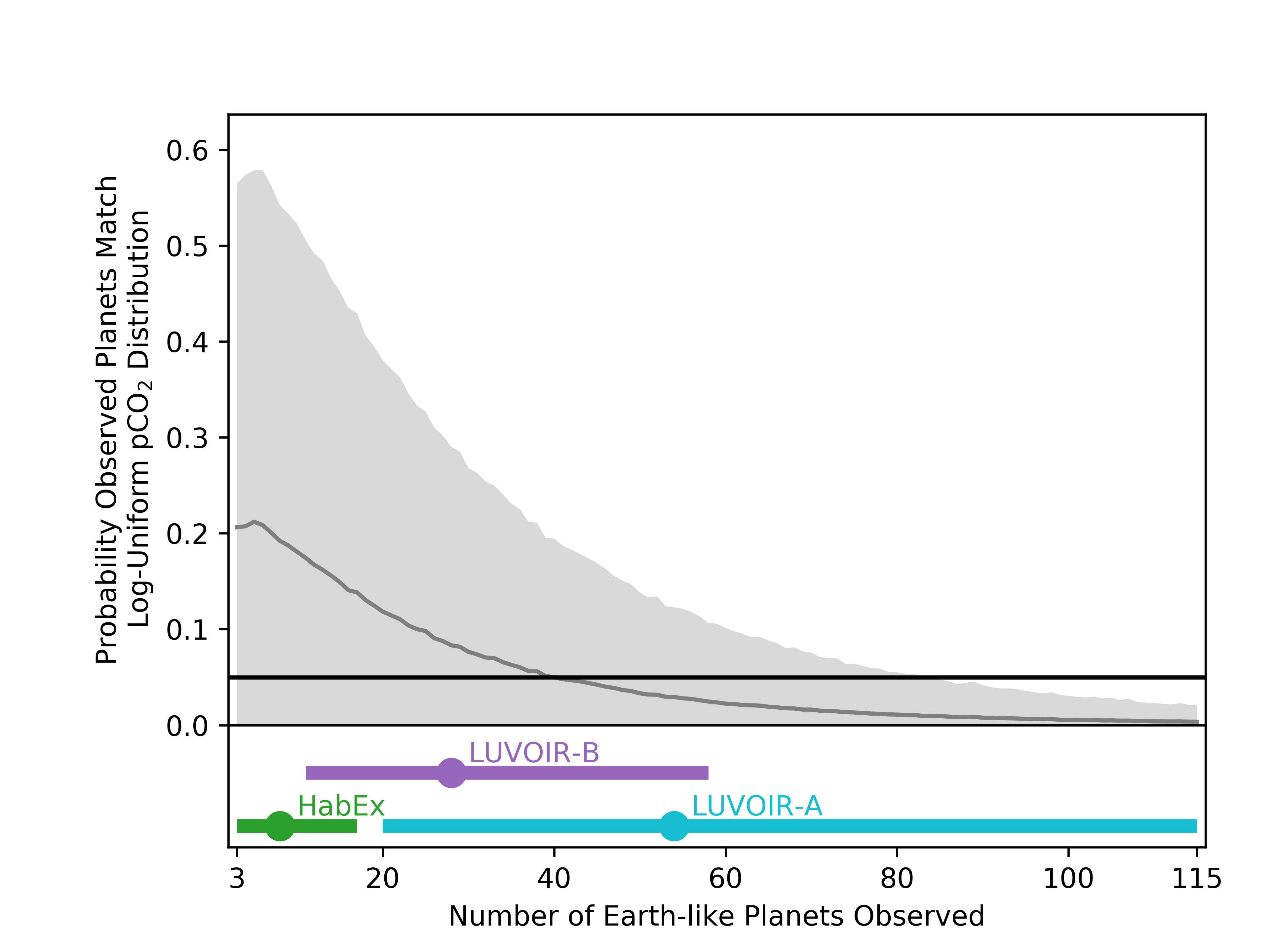
Figure 3: The probability observed exoplanets will accidentally match a log-uniform distribution for pCO₂ in the HZ if the true pCO₂ distribution is regulated by the carbonate-silicate weathering cycle, as shown in Figure 1. This probability is shown on the vertical axis. The horizontal axis shows the number of observed Earth-like exoplanets. The solid gray curve and corresponding shaded gray region shows the mean probability and $2\sigma$ uncertainty, respectively, that the observed planets, sampled from the planets shown in Figure 1, match a log-uniform pCO₂ distribution in the HZ. This curve is calculated from 10,000 two-dimensional Kolmogorov-Smirnov tests (see Results, subsection Observational uncertainty for pCO₂ in the HZ). The solid, horizontal black line highlights the 5% probability line. At the bottom of the figure, the labeled points and error bars show the number of Earth-like exoplanets the next generation of proposed space telescopes are expected to observe (telescope data in Table 1). The vertical scaling of the telescope points is arbitrary, only the horizontal position and extent of the $1{\sigma}$ error bars is significant. To rule out a log-uniform pCO₂ distribution with 95% confidence, future telescopes would need to observe at least 83 Earth-like planets.

A test of the two-dimensional phase space of $S$ and pCO₂ in the HZ is shown in Figure 3, which was produced using a two-dimensional Kolmogorov-Smirnov (KS) test. The two-dimensional KS test compares the statistical similarity of a sample distribution to a reference distribution [47, 48, 49]. For Figure 3, the reference distribution was comprised of 500 randomly generated planets from the log-uniform distribution for pCO₂ described above ($10^{-4}\leq$pCO${}_{2}\leq 10$ bar, $0.35\leq S\leq 1.05$ $S/S_{\oplus}$, and surface temperature between 248 and 355 K). The sample distribution was generated by randomly selecting a number of planets from Figure 1 equal to the number of observed exoplanets. For a given number of observed exoplanets in Figure 3, the horizontal axis, we ran the KS test 10,000 times then calculated the mean and standard deviation from those runs, shown by the gray contour and shaded region. This resampling is necessary as the two-dimensional KS test is a nonparametric approximation that two data sets come from the same underlying population [48]. We note that below ${\sim}$20 observed planets and for probabilities above ${\sim}$0.1, the two-dimensional KS test used here can be unreliable [49]. These limitations do not invalidate the analysis shown in Figure 3, as we want to know, with 95% confidence, that a log-uniform pCO₂ distribution can be ruled out if real exoplanets follow the distribution shown in Figure 1, which corresponds to the gray line and shaded contour dipping below the 0.05 probability value, shown by the horizontal black line, at 83 observations in Figure 3.

Telescope	Diameter [m]	Expected Yield ($1{\sigma}$)
HabEx	4	$8^{+9}_{-5}$
LUVOIR-B	8	$28^{+30}_{-17}$
LUVOIR-A	15	$54^{+61}_{-34}$

Table 2: The number of expected Earth-like exoplanets observed by each platform from the HabEx [30] and LUVOIR [31] final reports.

Thus, confidently detecting the carbonate-silicate weathering cycle will require many exoplanet observations, as shown in Figure 3. Proposed NASA telescopes, HabEx and LUVOIR, are expected to observe between 3 and 115 Earth-like exoplanets [31, 30] (see Table 2). The ranges for each mission concept are shown by the colored circles with error bars in Figure 3. Only the nominal capability of LUVOIR-A, the variant of the proposed LUVOIR space telescope with a primary mirror diameter of 15 m, would provide sufficient Earth-like exoplanet detections to confidently discriminate between a log-uniform pCO₂ distribution in the HZ and a pCO₂ distribution regulated by the carbonate-silicate weathering cycle. A caveat is that this calculation does not consider the instrument uncertainty in derived pCO₂ measurements for each telescope or that other processes not considered in our model may alter pCO₂ in the HZ, as discussed below.

3 Discussion

Our model assumes that the full variation and uncertainty in Earth’s carbon cycle parameters through time (Table 1) are representative of habitable Earth-like exoplanets generally. This assumption is a reasonable first-order approximation as the bulk composition and geochemistry of rocky exoplanets appear similar to Earth’s [50]. However, the validity of this assumption likely depends on the parameter in question. For example, it is probably reasonable to expect habitable exoplanets to have a wide range of land fractions and outgassing fluxes, but it is unclear whether there is as much natural variability in the temperature dependence of silicate weathering. An improved mechanistic understanding of weathering on Earth [51, 52] might reduce these uncertainties.

Other weathering feedbacks have been proposed to operate on the Earth through time, such as reverse weathering [53]. In reverse weathering, cations and dissolved silica released from silicate weathering are sequestered into clay minerals rather than carbonates so that CO₂ remains in the atmosphere, warming the climate and reducing ocean pH. Reverse weathering is thought to be strongly pH dependent and as ocean pH decreases, reverse weathering turns off, acting as a climate stabilization mechanism similar to the carbonate-silicate cycle. The importance of reverse weathering is so poorly constrained through Earth’s history [45] that it does not make sense to consider it in our model. However, with future constraints from geology and lab measurements, reverse weathering might alter the stable CO₂ abundances of our modeled atmospheres shown in Figure 1.

At both the inner and outer edges of the HZ, our model assumes that abundant liquid water exists at the planetary surface because, without a liquid surface ocean, the carbonate-silicate weathering cycle ceases and CO₂ cannot be sequestered after outgassing. Beyond these temperature bounds, other processes must regulate pCO₂. This is a caveat to consider in future observations. As we see from Figure 1, Mars has low atmospheric CO₂ and low incident flux. Frozen exoplanets similar to Mars, populating the white area under the 248 K contour in Figure 1, could exist in exoplanet surveys. Similarly, planets devoid of surface water, such as Venus, might exist at high pCO₂ within the HZ. If future observations detect such planets without confirming the existence of a liquid surface or surface temperature, it could introduce additional uncertainties in any relation between orbital distance and atmospheric CO₂. Detecting a surface ocean, one of the most important surface features to confirm when searching for biosignatures and habitability [54, 55, 56], is also important to interpret trends of CO₂ in the HZ.

Because we only consider variations on an Earth-like planet, our model predictions may underestimate the inherent variability in habitable exoplanetary conditions. Planets very different from the modern Earth, such as waterworlds without a carbonate-silicate weathering cycle [57] or CH₄-rich worlds [58, 59], could introduce additional uncertainty in an observed relationship between $S$ and pCO₂ in the HZ. Despite such uncertainties, future missions should measure the relationship between $S$ and pCO₂ in the HZ, or possibly a sharp transition in pCO₂ at the inner edge of the HZ due to loss of surface water and subsequent shutoff of surface weathering [60, 38]. A more complex model than presented here is necessary to predict such a jump in pCO₂ at the inner edge of the HZ. However, if the carbonate-silicate weathering cycle is indeed ubiquitous, as is typically assumed in HZ calculations, then the relationship between incident flux and pCO₂ may follow the $S$-pCO₂ relationship predicted in Figure 1. If no such relationship is observed, then the carbonate-silicate weathering cycle may have limited influence on planetary habitability and the limits of the conventional HZ could need revision. Alternatively, the HZ hypothesis could be incorrect and the long-term climate of HZ planets could be set by phenomena beyond those considered here.

A previous version of this work was published as part of a Ph.D. thesis [61].

4 Methods

4.1 Habitable zone 1D climate model

We use the Virtual Planetary Laboratory (VPL) 1D radiative-convective climate model[62, 5] to generate surface temperatures for an Earth-like planet at various pCO₂ and incident fluxes. We consider incident fluxes between 1.05$S_{\oplus}$ and $0.35S_{\oplus}$, the HZ limits for a Sun-like star [6], and atmospheric CO₂ partial pressures between $10^{-6}$ and 10 bar. We assume the atmosphere is comprised of CO₂ and H₂O. If the CO₂ partial pressure is below 1 bar, we set the initial atmospheric pressure to 1 bar and add N₂ to the atmosphere such that the total surface pressure is 1 bar. We fix the stratospheric water vapor concentration to the modern Earth value and follow the Manabe-Wetherald relative humidity distribution in the troposphere with empirical constraints based on the modern Earth [63].

Figure 4: The relative error between our 4${}^{\textrm{th}}$-order polynomial fit and the full 1D radiative-convective climate model. Our polynomial fit is valid between 1.05$S_{\oplus}$ and 0.35$S_{\oplus}$, where $S_{\oplus}$ is the Solar constant. The polynomial fit is valid for atmospheric CO₂ abundances between 10^-6 and 10 bar. The surface temperatures predicted by the polynomial fit reproduce the results of the 1D climate model. The maximum error in predicted surface temperature between the polynomial fit and the 1D climate model is ${\sim}$3%.

We fit the surface temperature output, $T_{\textrm{s}}$ in K, from the climate model with a 4${}^{\textrm{th}}$ order polynomial in $\ln(\textrm{pCO}_{2})$ and normalized stellar flux, as follows:

$$\begin{split}T_{\textrm{s}}\left(S,\textrm{pCO}_{2}\right)=4.809-222.0X-68.44X^{2}-6.737X^{3}-0.206X^{4}\\ +1414XY+446.4X^{2}Y+44.41X^{3}Y+1.364X^{4}Y\\ -2964XY^{2}-978.4X^{2}Y^{2}-98.86X^{3}Y^{2}-3.059X^{4}Y^{2}\\ +2655XY^{3}+907.5X^{2}Y^{3}+92.87X^{3}Y^{3}+2.892X^{4}Y^{3}\\ -868.4XY^{4}-304.6X^{2}Y^{4}-31.48X^{3}Y^{4}-0.985X^{4}Y^{4}\\ +1045Y-1496Y^{2}+1064Y^{3}-281.1Y^{4}.\end{split}$$ (8)

Here, CO₂ partial pressure pCO₂ is in bar, $X=\ln(\textrm{pCO}_{2})$, and $Y=S/S_{\oplus}$ is the incident flux, $S$, normalized to the solar constant, $S_{\oplus}$. Figure 4 shows the agreement between the 1D climate model and the polynomial fit used in this work.

4.2 Numerical carbonate-silicate cycle modeling

To calculate the steady-state pCO₂ in the atmospheres of Earth-like planets in the HZ, we use a weathering model that describes pCO₂ on the Earth through time[26, 21]. We summarize the model below and highlight how the model in this work differs from previous implementations[26, 21]. These previous implementations provide a comprehensive explanation and justification of the model parameterizations, and empirical and theoretical basis. The model, as a Python script, is available in the Supplementary Data and contains a complete description of the model equations and parameters (see the file weathering_model.py).

The weathering model balances the flux of outgassed CO₂ against the loss of carbon due to continental and seafloor weathering, which result in precipitation of carbonates in the ocean and seafloor pore space. Quantitatively, for time $t$, this is described by time-dependent equations where we normalize to the mass of the ocean, $M_{\textrm{o}}$ (nominally, an Earth ocean, $1.35\times 10^{21}$ kg):

$$\begin{split}\frac{dC}{dt}&=\frac{F_{\textrm{out}}+F_{\textrm{carb}}-P_{\textrm{o}}-P_{\textrm{p}}}{M_{\textrm{o}}}\\ \frac{dA}{dt}&=2\cdot\frac{F_{\textrm{sil}}+F_{\textrm{carb}}+F_{\textrm{diss}}-P_{\textrm{o}}-P_{\textrm{p}}}{M_{\textrm{o}}}.\end{split}$$ (9)

Here, $C$ is the non-organic carbon content of the atmosphere-ocean system in mol C kg^-1, and $A$ is the carbonate alkalinity in mol equivalents (mol eq). Carbonate alkalinity (henceforth alkalinity) is the charge-weighted sum of the mol liter^-1 concentration of bicarbonate and carbonate anions, [HCO${}_{3}^{-}$] + 2[CO${}_{3}^{2-}$]. $F_{\textrm{out}}$ is the global CO₂ outgassing flux, $F_{\textrm{carb}}$ and $F_{\textrm{sil}}$ are the continental carbonate and silicate weathering fluxes, $F_{\textrm{diss}}$ is the rate of seafloor basalt dissolution, and $P_{\textrm{p}}$ and $P_{\textrm{o}}$ are the pore and ocean precipitation fluxes. The fluxes on the right-hand side of equation 9 ($F_{\textrm{out}}$, $F_{\textrm{carb}}$, $P_{\textrm{o}}$, $P_{\textrm{p}}$, $F_{\textrm{sil}}$, $F_{\textrm{carb}}$, and $F_{\textrm{diss}}$) are given in mol C yr^-1 for $dC/dt$ and in mol eq yr^-1 for $dA/dt$.

The alkalinity that enters the ocean from weathering will balance a $+2$ charge cation (e.g. Ca⁺⁺), which is why a factor of $2$ enters in the definition of $dA/dt$ in equation 9. Hence, geochemists often think of alkalinity in terms of the balance of cations produced in weathering, principally Ca⁺⁺. This reasoning arises because the weighted sum of carbonate and bicarbonate concentrations must balance the charge of conservative cations minus conservative anions (i.e., 2[Ca⁺⁺] + 2[Mg⁺⁺] + Na⁺ +… - [Cl^-] - …), ignoring minor contributions from weak acid anions and water dissociation. Weathering releases cations and carbon speciation adjusts to ensure charge balance, so that the cation release is effectively equivalent to carbonate alkalinity.

To improve the rate of model convergence and range of model inputs over which equation 9 converges, we do not consider the seafloor pore space and atmosphere-ocean as separate systems. This differs from previous versions of the model[21], which considered the atmosphere-ocean and pore space independently. Rather, we approximate the atmosphere-ocean and pore space as a single entity in equation 9. This simplification does not appreciably change the model output for atmospheric CO₂ because we run the model to steady-state in all cases, where the atmosphere-ocean and pore space reach approximate equilibrium. In the next section, we present additional details on our model implementation and discuss the agreement between our no-pore model and the original, two-box model[21].

A second modification is the range of incident stellar fluxes over which the model can be run. Previously, the model described here was used to study the Earth through time[21] and thus only considered solar fluxes between $S_{\oplus}$ (the modern solar constant) and early Earth’s $0.7S_{\oplus}$ ($S_{\oplus}=1360$ W m^-2). We extend that range to include the entire conservative HZ of a Sun-like star, roughly 1.05$S_{\oplus}$ to 0.35$S_{\oplus}$ [6]. We use equation 8, the 4${}^{\textrm{th}}$-order polynomial fit to a 1D climate model, to calculate surface temperatures throughout the HZ. The Bond albedo of the planet is calculated dynamically by the climate model and thus included implicitly in our polynomial fit.

With the coupled climate and weathering model, we generate steady-state, Earth-like planets by randomly sampling plausible initial model inputs. The ranges for each parameter we consider are representative of the Earth through time[21] and shown in Table 1. These ranges represent very broad uncertainties of the carbonate-silicate cycle on the Earth through time and so are appropriate for Earth-like planets. We conservatively assume a uniform distribution for each parameter range shown in Table 1.

We parameterize the internal heat of an Earth-like planet conservatively using the planet’s age, ranging 0 to 10 Gyr, which is the approximate habitable lifetime of an Earth-like planet around a Sun-like star [64]. The equation for planetary heat relative to the modern Earth, $Q$, is given by

$$Q=\left(1-\frac{4.5-\tau}{4.5}\right)^{-n_{\textrm{out}}}$$ (10)

where $\tau$ is the age of the planet in Gyr, and $n_{\textrm{out}}$ is the scaling exponent for internal heat, with a range given in Table 1.

The parameter ranges shown in Table 1 represent the uncertainty of the carbonate-silicate weathering cycle on the Earth through time [21]. Implicit in our assumed parameter ranges is that continental land fraction, $f_{\textrm{land}}$, and biological weathering fraction, $f_{\textrm{bio}}$, have increased from 0 when the Earth formed to 1 on the modern Earth. Similarly, the relative internal heat, $Q$, is assumed to be large when the Earth is young and unity for the modern Earth. Therefore, on the modern Earth, where $f_{\textrm{land}}=1$, $f_{\textrm{bio}}=1$, and $Q=1$, the weathering rate is maximized and outgassing rate is relatively small (see Methods, subsection Validity of carbon cycle parameterizations to exoplanets for a discussion on the importance of these three parameters in our model). This is seen in Figure 1, where the modern Earth appears near the lower bound for predicted pCO₂ in the HZ. If the continents on an exoplanet were more easily weathered or outgassing much lower than on the modern Earth, such exoplanets could have pCO₂ values well below the modern Earth value shown in Figure 1. We do not consider such exoplanets in this model, so the results presented here are only applicable to planets similar to the Earth through time.

Our model assumes that each simulated planet is habitable, i.e., it has a stable, liquid surface ocean, a necessity for the carbonate-silicate cycle to operate. For a mean surface temperature below 248 K, Earth-like planets are likely completely frozen [36], which we use as a lower temperature bound in the model. While 248 K is below the freezing point of water, it is a global mean surface temperature and 3D models show that the range 248-273 K for this parameter does not preclude the existence of a liquid ocean belt near the equator. At the other temperature extreme, a hot, Earth-like planet can rapidly lose its surface oceans due to high atmospheric water vapor concentrations that are photolyzed and subsequently lost to space. This upper temperature bound on habitability occurs at ${\sim}355$ K [37]. Above 355 K, Earth-like planets are unlikely to remain habitable for more than ${\sim}1$ Gyr [37] and cannot operate a carbonate-silicate cycle over geologic timescales. We use these two temperature bounds, 248 K and 355 K, as the limits for habitability in our model. Any modeled planet with a final surface temperature outside these limits is uninhabitable and removed from our results.

We limit HZ planets to those with pCO₂ below 10 bar. For most Earth-like planets in the HZ, 10 bar of CO₂ results in planets with surface temperatures well above 355 K, which are not habitable on long time scales. If we impose a fixed stratospheric water vapor concentration in the 1D climate model and modify the tropospheric water vapor concentration based on empirical data from the modern Earth, we enable the 1D climate model to accurately model habitable, Earth-like planets through much of the HZ. But in the outer HZ, with more than ${\sim}$10 bar of CO₂, this assumption overestimates atmospheric water vapor concentrations and leads to artificially warm planets, so we reject such cases. Above ${\sim}$10 bar of CO₂ in the outer HZ, assuming a saturated troposphere for water vapor, increasing atmospheric CO₂ may not lead to additional warming[6]. Rather, the surface cools in such scenarios because additional CO₂ leads to increased Rayleigh scattering and no additional warming. Because Earth-like planets in the outer HZ would be frozen and uninhabitable even with CO₂ partial pressures above ${\sim}$10 bar, we impose a 10 bar limit for CO₂ in the outer HZ. This limit agrees with previous CO₂ limitations in coupled climate and weathering models[29].

4.3 Combined ocean and pore space model justification

The carbon cycle model used in this work was previously derived as a two-box model[21], where the atmosphere-ocean and the seafloor pore space were separated. In this work, we combine the ocean-atmosphere and the pore space into a single unit. This modification can be implemented in the original model[21] by assuming that the pH of the pore space is the same as the pH of the ocean, and assuming that the alkalinity and carbon content of the ocean and pore space are the same. The dissolution and precipitation fluxes can then be calculated without treating the ocean-atmosphere and the pore space as different systems. This modification allows the model to converge quicker over a wider range of parameter combinations.

To validate our combined model, we ran the modern Earth through both the original, two-box model[21] and our modified model at 10 different incident fluxes between $S_{\oplus}$ and 0.7$S_{\oplus}$. The average error in predicted CO₂ values between our model and the two-box model was 2.8%, with a minimum error of 2.3%, and a maximum error of 3.6%. Given the large uncertainties in model inputs (Table 1), the few percent error introduced by our simplified model is unimportant.

For each parameter combination in our simplified model, we start with the modern Earth then impose a step change for each model parameter. We then run the simulation for 10 Gyr or until the system reaches steady-state. We consider the model to have reached steady-state when extrapolation of the rate of change of pCO₂ for 1 Gyr changes pCO₂ by less than 1%. Typically, the model converges within a few Myr to a few tens of Myr. Rarely (2 of the 1200 planets simulated in this work), parameter combinations will not reach steady-state after 10 Gyr. Simulations with combinations of exceptionally high outgassing rates and low CO₂ weathering rates can enter a regime were atmospheric CO₂ builds without bound, never converging. Such model results are beyond the range of validity of our model.

4.4 Validity of carbon cycle parameterizations to exoplanets

The parameterization of weathering in our model has been empirically validated for the modern Earth [16, 26, 21]. The exponential temperature-dependence of continental weathering is a reasonable approximation that agrees with field and lab measurements [16] and can reproduce the climate results of more complex models [26, 21]. Similarly, the power-law parameterization for the pCO₂-dependence of continental weathering agrees with data from the modern Earth [26] and can even be approximately derived from equilibrium chemistry arguments for an Earth-like exoplanet [38]. The bulk geochemistry of rocky exoplanets may be similar to Earth’s [50], so we expect our weathering parameterization to reasonably approximate Earth-like planets in the HZ. However, uncertainties in how the carbonate-silicate weathering cycle regulates climate on Earth persist [21], so the predicted variations in pCO₂ in our model may not capture the true variability of pCO₂ in the HZ. Below, we show that our broad parameterization of the carbonate-silicate weathering cycle may encompass the plausible range of pCO₂ for the Earth through time, but improved understanding the carbonate-silicate weathering cycle may be necessary to know if such variations are indeed representative of the Earth through time and applicable to Earth-like planets generally.

The rate of weathering depends strongly on the intrinsic features of a planet, such as the CO₂ outgassing rate and the properties of its continents. Changes in continental uplift rate, lithology, and configuration are parameterized in our model through the $f_{\textrm{land}}$ and $f_{\textrm{bio}}$ terms. The parameters $f_{\textrm{land}}$ and $f_{\textrm{bio}}$ linearly scale the weathering flux and could analogously be considered a continental weatherability scaling factor. For the ranges of $f_{\textrm{land}}$ and $f_{\textrm{bio}}$ considered in our model (see Table 1), changes in the continental weatherability alone can generate pCO₂ values spanning ${\sim}4$ orders of magnitude. This broad parameterization likely encompasses pCO₂ perturbations due to continental weatherability changes caused by large volcanic eruptions or changes in continental configuration. Indeed, the largest, constrained change in pCO₂ due to such events on Earth may be closer to ${\sim}1$ order of magnitude, coeval with the eruption of the Siberian Traps [65].

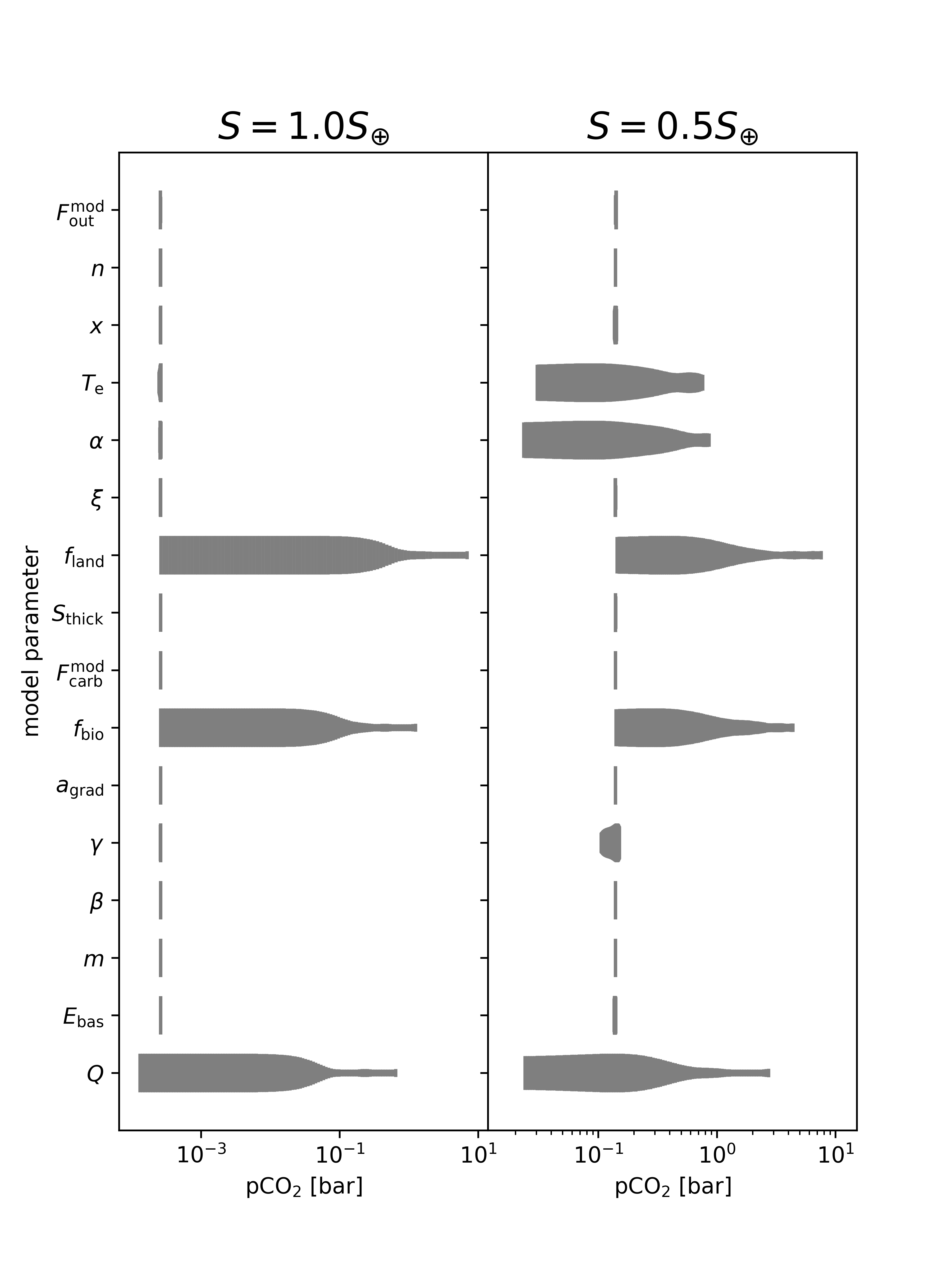
Figure 5: The spread in steady-state pCO₂ from varying a single model parameter. Each parameter in Table 1 is shown on the vertical axis (note that $n_{\textrm{out}}$ and $\tau$ are incorporated into $Q$, see equation 10). The left panel shows an incident flux of $S=1.0S_{\oplus}$. The right panel shows an incident flux of $S=0.5S_{\oplus}$. For each parameter, we held all other parameters constant at the modern Earth value (see text) and randomly sampled 100 values for the parameter in question from uniform distributions of the ranges given in Table 1. The horizontal extent of the gray shaded region shows the range of possible pCO₂ values when all other parameters are fixed. The thickness of each gray shaded region shows the relative abundance of steady-state planets at that pCO₂. The thickest regions show maximum relative abundance, the thinnest regions show the minimum relative abundance. No surface temperature limits on habitability were imposed for the simulated planets. At low pCO₂, three parameters ($f_{\textrm{land}}$, $f_{\textrm{bio}}$, and $Q$) dominate the spread in pCO₂. At higher pCO₂, the temperature- and pCO₂-dependence of continental silicate weathering ($T_{\textrm{e}}$ and $\alpha$) are also important.

The importance of continental weatherability ($f_{\textrm{land}}$ and $f_{\textrm{bio}}$) on pCO₂, relative to other parameters, is shown in Figure 5. Figure 5 was generated by sampling uniform distributions for each model parameter shown in Table 1 across its listed range. When one parameter was varied, all other parameters were held constant at their modern Earth value, which we define as: $F_{\textrm{mod}}^{\textrm{out}}=6$ Tmol C yr^-1, $n=1.75$, $x=1$, $T_{\textrm{e}}=25$ K, $\alpha=0.3$, $\xi=0.3$, $f_{\textrm{land}}=1$, $S_{\textrm{thick}}=1$, $F^{\textrm{mod}}_{\textrm{carb}}=10$ Tmol C yr^-1, $f_{\textrm{bio}}=1$, $a_{\textrm{grad}}=1.075$, $\gamma=0.2$, $\beta=0.1$, $m=1.5$, $E_{\textrm{bas}}=90$ kJ mol^-1, and $Q=1$. Note that we incorporate $n_{\textrm{out}}$ and $\tau$ from Table 1 into $Q$, the internal heat (see equation 10), which is the parameter of interest. We show two different values for $S$ in Figure 5, $S=1.0S_{\oplus}$ in the left panel and $S=0.5S_{\oplus}$ in the right panel. For both values of $S$, Figure 5 shows that variations in $f_{\textrm{land}}$ and $f_{\textrm{bio}}$ alone can alter pCO₂ by orders of magnitude.

The internal heat of the planet, $Q$, plays a similarly important role in setting pCO₂. The rate of CO₂ outgassing is determined by $Q$ and our broad parameterization of $Q$ allows pCO₂ to vary by orders of magnitude throughout the HZ, as shown in Figure 5.

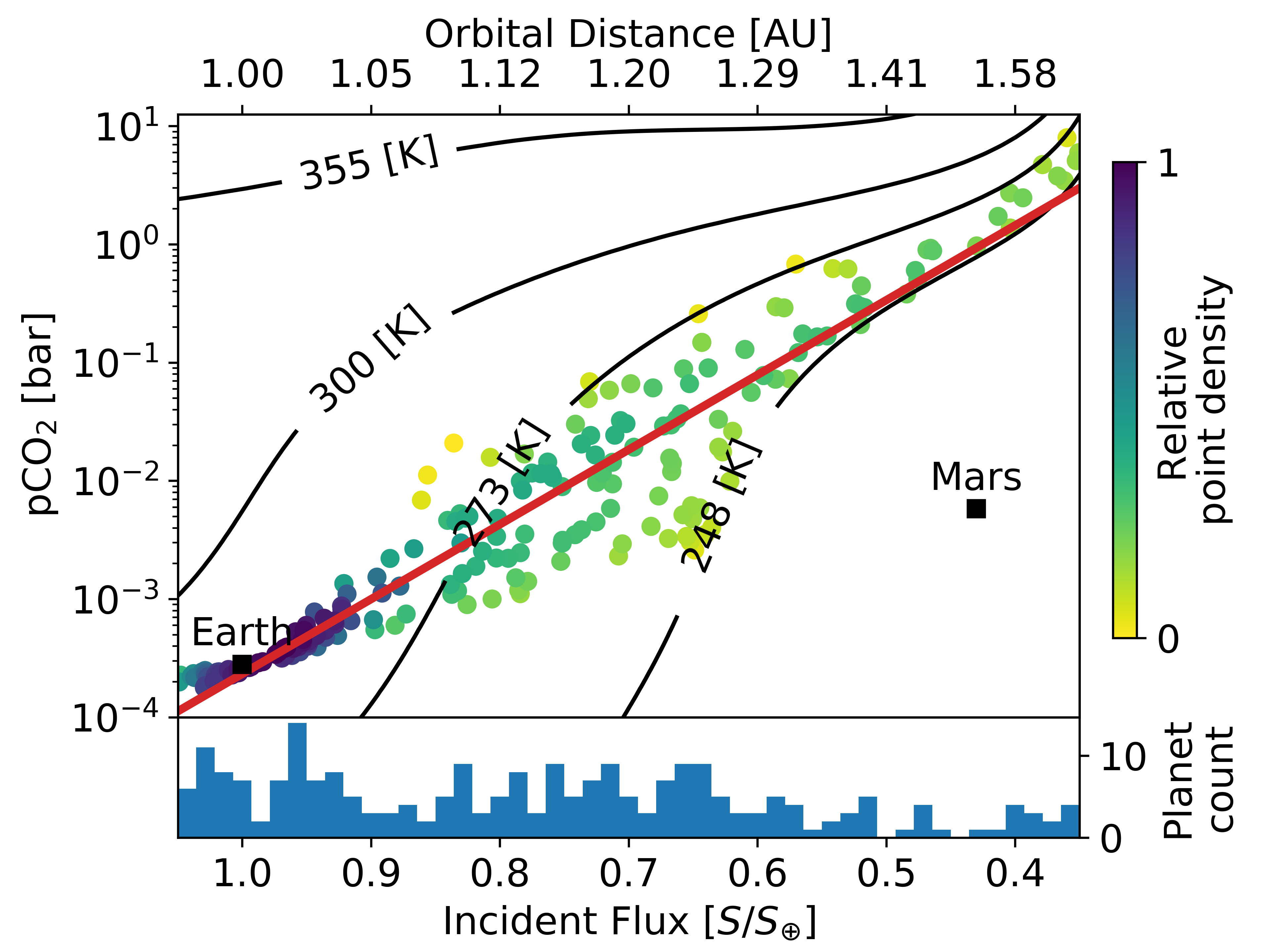
Figure 6: The expected distribution of stable, steady-state pCO₂ on Earth-like planets if $Q$, $f_{\textrm{land}}$, and $f_{\textrm{bio}}$ are fixed to 1, i.e., modern Earth values. Except for fixing $Q=f_{\textrm{land}}=f_{\textrm{bio}}=1$, this figure is generated identically to Figure 1. The spread in pCO₂ in the outer HZ is due to the temperature- and pCO₂-dependence of continental weathering ($T_{\textrm{e}}$ and $\alpha$). This is expected from equation 4, which shows that $T_{\textrm{e}}$ and $\alpha$ will be increasingly influential as pCO₂ and surface temperature deviate from the modern Earth values, as discussed in the Results, subsection Habitable zone climate theory revisited. Without changes in $Q$, $f_{\textrm{land}}$, and $f_{\textrm{bio}}$, there is little spread in pCO₂ in the inner HZ.

The rate of CO₂ outgassing and continental weatherability drive the majority of the spread in pCO₂ shown in Figure 1. This is readily seen in Figure 6, which shows the results of 300 random parameter combinations from uniform distributions of the parameters in Table 1 except for $Q$, $f_{\textrm{land}}$, and $f_{\textrm{bio}}$, which were all fixed to 1. Of the 300 parameter combinations, 235 remained above 248 K and are shown in Figure 6. Comparing Figure 6 to Figure 1, it is readily apparent that the broad uncertainty in pCO₂ from our results is due to variations in intrinsic planetary properties ($Q$, $f_{\textrm{land}}$, and $f_{\textrm{bio}}$) rather than uncertainties in the tuning parameters of our carbon cycle parameterization.

The outgassing rate and continental properties of habitable exoplanets remain unknown. Thus, our broad parameterization of those terms, which align with possible conditions on Earth throughout its history, are a reasonable approximation. If an Earth-like, carbonate-silicate weathering cycle is common on habitable planets, then these parameters may largely determine pCO₂ on such planets and generate a range for pCO₂ at a given orbital distance similar to that shown in Figure 1.

Data Availability

The data used in this work is available in the Supplementary Data. Our model code depends on the location of the data directory, so the data and model are provided together in a single, zipped file.

Code Availability

The code used to generate the data and figures for this work is available in the Supplementary Data.

References

- [1] Newton, I. Philosophiæ Naturalis Principia Mathematica (Royal Society, London, 1687).
- [2] Cohen, I. B., Whitman, A. & Budenz, J. The Principia: Mathematical Principles of Natural Philosophy (University of California Press, 1999), 1 edn. URL https://www.jstor.org/stable/10.1525/j.ctt9qh28z.
- [3] Whewell, W. Of the Plurality of Worlds: An Essay (London : J.W. Parker and Son, 1853).
- [4] Kasting, J. F. Earth’s early atmosphere. Science 259, 920–926 (1993). URL https://doi.org/10.1126/science.11536547.
- [5] Catling, D. C. & Kasting, J. F. Atmospheric Evolution on Inhabited and Lifeless Worlds (Cambridge University Press, New York, 2017).
- [6] Kopparapu, R. K. et al. Habitable Zones around Main-sequence Stars: New Estimates. The Astrophysical Journal 765, 131 (2013). URL http://stacks.iop.org/0004-637X/765/i=2/a=131.
- [7] Kasting, J. F., Whitmire, D. P. & Reynolds, R. T. Habitable Zones around Main Sequence Stars. Icarus 101, 108–128 (1993). URL http://www.sciencedirect.com/science/article/pii/S0019103583710109.
- [8] Stevenson, D. J. Life-sustaining planets in interstellar space? Nature 400, 32–32 (1999). URL https://doi.org/10.1038/21811.
- [9] Seager, S. Exoplanet Habitability. Science 340, 577–581 (2013). URL https://doi.org/10.1126/science.1232226.
- [10] Krissansen-Totton, J., Olson, S. & Catling, D. C. Disequilibrium biosignatures over Earth history and implications for detecting exoplanet life. Science Advances 4, eaao5747 (2018). URL https://advances.sciencemag.org/content/4/1/eaao5747.
- [11] Wogan, N., Krissansen-Totton, J. & Catling, D. C. Abundant Atmospheric Methane from Volcanism on Terrestrial Planets Is Unlikely and Strengthens the Case for Methane as a Biosignature. The Planetary Science Journal 1, 58 (2020). URL https://iopscience.iop.org/article/10.3847/PSJ/abb99e/meta. Publisher: IOP Publishing.
- [12] Abe, Y., Abe-Ouchi, A., Sleep, N. H. & Zahnle, K. J. Habitable Zone Limits for Dry Planets. Astrobiology 11, 443–460 (2011). URL https://www.liebertpub.com/doi/full/10.1089/ast.2010.0545.
- [13] Zsom, A., Seager, S., Wit, J. d. & Stamenković, V. Toward the Minimum Inner Edge Distance of The Habitable Zone. The Astrophysical Journal 778, 109 (2013). URL https://doi.org/10.1088/0004-637X/778/2/109.
- [14] Yang, J., Boué, G., Fabrycky, D. C. & Abbot, D. S. Strong Dependence of the Inner Edge of the Habitable Zone on Planetary Rotation Rate. The Astrophysical Journal Letters 787, L2 (2014). URL http://stacks.iop.org/2041-8205/787/i=1/a=L2.
- [15] Way, M. J. et al. Was Venus the first habitable world of our solar system? Geophysical Research Letters 43, 2016GL069790 (2016). URL http://onlinelibrary.wiley.com/doi/10.1002/2016GL069790/abstract.
- [16] Walker, J. C. G., Hays, P. B. & Kasting, J. F. A negative feedback mechanism for the long-term stabilization of Earth’s surface temperature. Journal of Geophysical Research: Oceans 86, 9776–9782 (1981). URL https://doi.org/10.1029/JC086iC10p09776.
- [17] Sagan, C. & Mullen, G. Earth and Mars: Evolution of Atmospheres and Surface Temperatures. Science 177, 52–56 (1972). URL https://doi.org/10.1126/science.177.4043.52.
- [18] Tajika, E. & Matsui, T. Evolution of terrestrial proto-CO2 atmosphere coupled with thermal history of the earth. Earth and Planetary Science Letters 113, 251–266 (1992). URL https://linkinghub.elsevier.com/retrieve/pii/0012821X9290223I.
- [19] Tajika, E. & Matsui, T. Degassing history and carbon cycle of the Earth: From an impact-induced steam atmosphere to the present atmosphere. Lithos 30, 267–280 (1993). URL https://linkinghub.elsevier.com/retrieve/pii/002449379390040J.
- [20] Sleep, N. H. & Zahnle, K. Carbon dioxide cycling and implications for climate on ancient Earth. Journal of Geophysical Research: Planets 106, 1373–1399 (2001). URL http://agupubs.onlinelibrary.wiley.com/doi/abs/10.1029/2000JE001247.
- [21] Krissansen-Totton, J., Arney, G. N. & Catling, D. C. Constraining the climate and ocean pH of the early Earth with a geological carbon cycle model. Proceedings of the National Academy of Sciences 2017–21296 (2018). URL https://doi.org/10.1073/pnas.1721296115.
- [22] Ebelmen, J.-J. Sur les produits de la décomposition des espèces minérales de la famille des silicates. In Annales des Mines, vol. 7, 66 (1845). Issue: 3.
- [23] Walker, J. C. G. Biogeochemical Cycles of Carbon on a Hierarchy of Time Scales. In Oremland, R. S. (ed.) Biogeochemistry of Global Change: Radiatively Active Trace Gases Selected Papers from the Tenth International Symposium on Environmental Biogeochemistry, San Francisco, August 19–24, 1991, 3–28 (Springer US, Boston, MA, 1993). URL https://doi.org/10.1007/978-1-4615-2812-8_1.
- [24] Berner, R. A. The Phanerozoic Carbon Cycle: CO2 and O2 (Oxford University Press, New York, NY, 2004).
- [25] Mills, B., Daines, S. J. & Lenton, T. M. Changing tectonic controls on the long-term carbon cycle from Mesozoic to present. Geochemistry, Geophysics, Geosystems 15, 4866–4884 (2014). URL http://agupubs.onlinelibrary.wiley.com/doi/abs/10.1002/2014GC005530.
- [26] Krissansen-Totton, J. & Catling, D. C. Constraining climate sensitivity and continental versus seafloor weathering using an inverse geological carbon cycle model. Nature Communications 8, 15423 (2017). URL https://www.nature.com/articles/ncomms15423.
- [27] Hakim, K. et al. Lithologic Controls on Silicate Weathering Regimes of Temperate Planets. arXiv:2008.11620 [astro-ph] (2020). URL http://arxiv.org/abs/2008.11620. ArXiv: 2008.11620.
- [28] Coogan, L. A. & Dosso, S. E. Alteration of ocean crust provides a strong temperature dependent feedback on the geological carbon cycle and is a primary driver of the Sr-isotopic composition of seawater. Earth and Planetary Science Letters 415, 38–46 (2015). URL https://linkinghub.elsevier.com/retrieve/pii/S0012821X15000485.
- [29] Kadoya, S. & Tajika, E. Conditions for oceans on earth-like planets orbiting within the habitable zone: importance of volcanic CO2 degassing. The Astrophysical Journal 790, 107 (2014). URL https://doi.org/10.1088/0004-637X/790/2/107.
- [30] HabEx. Habitable Exoplanet Observatory (HabEx) Final Report. Tech. Rep., NASA (2019). URL https://www.jpl.nasa.gov/habex/documents/.
- [31] LUVOIR. Large UV/Optical/IR Surveyor (LUVOIR) Final Report. Tech. Rep., NASA (2019). URL https://asd.gsfc.nasa.gov/luvoir/reports/.
- [32] Bean, J. L., Abbot, D. S. & Kempton, E. M.-R. A Statistical Comparative Planetology Approach to the Hunt for Habitable Exoplanets and Life Beyond the Solar System. The Astrophysical Journal 841, L24 (2017). URL https://doi.org/10.3847/2041-8213/aa738a.
- [33] Checlair, J. H. et al. A Statistical Comparative Planetology Approach to Maximize the Scientific Return of Future Exoplanet Characterization Efforts. arXiv:1903.05211 [astro-ph] (2019). URL http://arxiv.org/abs/1903.05211. ArXiv: 1903.05211.
- [34] Turbet, M. Two examples of how to use observations of terrestrial planets orbiting in temperate orbits around low mass stars to test key concepts of planetary habitability. Proceedings of the Annual meeting of the French Society of Astronomy and Astrophysics SF2A-2019, pp. 341–346 (2019).
- [35] Abbot, D. S., Cowan, N. B. & Ciesla, F. J. Indication of Insensitivity of Planetary Weathering Behavior and Habitable Zone to Surface Land Fraction. The Astrophysical Journal 756, 178 (2012). URL http://stacks.iop.org/0004-637X/756/i=2/a=178.
- [36] Charnay, B. et al. Exploring the faint young Sun problem and the possible climates of the Archean Earth with a 3-D GCM. Journal of Geophysical Research: Atmospheres 118, 10,414–10,431 (2013). URL https://doi.org/10.1002/jgrd.50808.
- [37] Wolf, E. T., Shields, A. L., Kopparapu, R. K., Haqq-Misra, J. & Toon, O. B. Constraints on Climate and Habitability for Earth-like Exoplanets Determined from a General Circulation Model. The Astrophysical Journal 837, 107 (2017). URL https://doi.org/10.3847/1538-4357/aa5ffc.
- [38] Graham, R. J. & Pierrehumbert, R. Thermodynamic and Energetic Limits on Continental Silicate Weathering Strongly Impact the Climate and Habitability of Wet, Rocky Worlds. The Astrophysical Journal 896, 115 (2020). URL https://doi.org/10.3847%2F1538-4357%2Fab9362. Publisher: American Astronomical Society.
- [39] Kasting, J. F. & Toon, O. B. Climate evolution on the terrestrial planets. In Origin and evolution of planetary and satellite atmospheres, 423–449 (University of Arizona Press, Tucson, AZ, 1989). URL http://inis.iaea.org/Search/search.aspx?orig_q=RN:21012339.
- [40] Budyko, M. I. The effect of solar radiation variations on the climate of the Earth. Tellus 21, 611–619 (1969). URL https://doi.org/10.3402/tellusa.v21i5.10109.
- [41] Koll, D. D. B. & Cronin, T. W. Earth’s outgoing longwave radiation linear due to H O greenhouse effect. Proceedings of the National Academy of Sciences 115, 10293–10298 (2018). URL http://www.pnas.org/lookup/doi/10.1073/pnas.1809868115.
- [42] Myhre, G., Highwood, E. J., Shine, K. P. & Stordal, F. New estimates of radiative forcing due to well mixed greenhouse gases. Geophysical Research Letters 25, 2715–2718 (1998). URL http://doi.wiley.com/10.1029/98GL01908.
- [43] Pierrehumbert, R. T. Principles of Planetary Climate (Cambridge University Press, Cambridge, UK, 2010), 3rd edn.
- [44] Charnay, B., Le Hir, G., Fluteau, F., Forget, F. & Catling, D. C. A warm or a cold early Earth? New insights from a 3-D climate-carbon model. Earth and Planetary Science Letters 474, 97–109 (2017). URL https://linkinghub.elsevier.com/retrieve/pii/S0012821X17303394.
- [45] Krissansen-Totton, J. & Catling, D. C. A coupled carbon-silicon cycle model over Earth history: Reverse weathering as a possible explanation of a warm mid-Proterozoic climate. Earth and Planetary Science Letters 537, 116181 (2020). URL https://linkinghub.elsevier.com/retrieve/pii/S0012821X20301242.
- [46] Kadoya, S., Krissansen-Totton, J. & Catling, D. C. Probable Cold and Alkaline Surface Environment of the Hadean Earth Caused by Impact Ejecta Weathering. Geochemistry, Geophysics, Geosystems 21, e2019GC008734 (2020). URL http://agupubs.onlinelibrary.wiley.com/doi/abs/10.1029/2019GC008734.
- [47] Peacock, J. A. Two-dimensional goodness-of-fit testing in astronomy. Monthly Notices of the Royal Astronomical Society 202, 615–627 (1983). URL https://academic.oup.com/mnras/article/202/3/615/967854. Publisher: Oxford Academic.
- [48] Fasano, G. & Franceschini, A. A multidimensional version of the Kolmogorov–Smirnov test. Monthly Notices of the Royal Astronomical Society 225, 155–170 (1987). URL https://academic.oup.com/mnras/article/225/1/155/1007281. Publisher: Oxford Academic.
- [49] Press, W. H. & Teukolsky, S. A. Kolmogorov-Smirnov Test for Two-Dimensional Data. Computers in Physics 2, 74 (1988). URL http://scitation.aip.org/content/aip/journal/cip/2/4/10.1063/1.4822753.
- [50] Doyle, A. E., Young, E. D., Klein, B., Zuckerman, B. & Schlichting, H. E. Oxygen fugacities of extrasolar rocks: Evidence for an Earth-like geochemistry of exoplanets. Science 366, 356 (2019). URL http://science.sciencemag.org/content/366/6463/356.abstract.
- [51] Maher, K. & Chamberlain, C. P. Hydrologic Regulation of Chemical Weathering and the Geologic Carbon Cycle. Science 343, 1502–1504 (2014). URL https://doi.org/10.1126/science.1250770.
- [52] Winnick, M. J. & Maher, K. Relationships between CO2, thermodynamic limits on silicate weathering, and the strength of the silicate weathering feedback. Earth and Planetary Science Letters 485, 111–120 (2018). URL https://linkinghub.elsevier.com/retrieve/pii/S0012821X18300098.
- [53] Isson, T. T. & Planavsky, N. J. Reverse weathering as a long-term stabilizer of marine pH and planetary climate. Nature 560, 471–475 (2018). URL https://www.nature.com/articles/s41586-018-0408-4.
- [54] Lustig-Yaeger, J. et al. Detecting Ocean Glint on Exoplanets Using Multiphase Mapping. The Astronomical Journal 156, 301 (2018). URL https://doi.org/10.3847%2F1538-3881%2Faaed3a.
- [55] Robinson, T. D., Meadows, V. S. & Crisp, D. Detecting Oceans on Extrasolar Planets Using the Glint Effect. The Astrophysical Journal 721, L67–L71 (2010). URL https://doi.org/10.1088/2041-8205/721/1/L67.
- [56] Williams, D. M. & Gaidos, E. Detecting the glint of starlight on the oceans of distant planets. Icarus 195, 927–937 (2008). URL https://linkinghub.elsevier.com/retrieve/pii/S0019103508000407.
- [57] Kite, E. S. & Ford, E. B. Habitability of Exoplanet Waterworlds. The Astrophysical Journal 864, 75 (2018). URL https://doi.org/10.3847%2F1538-4357%2Faad6e0.
- [58] Haqq-Misra, J. D., Domagal-Goldman, S. D., Kasting, P. J. & Kasting, J. F. A Revised, Hazy Methane Greenhouse for the Archean Earth. Astrobiology 8, 1127–1137 (2008). URL https://doi.org/10.1089/ast.2007.0197.
- [59] Wordsworth, R. et al. Transient reducing greenhouse warming on early Mars. Geophysical Research Letters 44, 665–671 (2017). URL http://agupubs.onlinelibrary.wiley.com/doi/abs/10.1002/2016GL071766.
- [60] Turbet, M., Ehrenreich, D., Lovis, C., Bolmont, E. & Fauchez, T. The runaway greenhouse radius inflation effect. An observational diagnostic to probe water on Earth-size planets and test the habitable zone concept. Astronomy & Astrophysics (2019). URL https://www.aanda.org/articles/aa/abs/forth/aa35585-19/aa35585-19.html.
- [61] Lehmer, O. R. The Formation and Evolution of Habitable Worlds. Ph.D. thesis, University of Washington, Seattle, WA (2020). URL http://hdl.handle.net/1773/45656.
- [62] Meadows, V. S. et al. The Habitability of Proxima Centauri b: Environmental States and Observational Discriminants. Astrobiology 18, 133–189 (2018). URL https://www.liebertpub.com/doi/full/10.1089/ast.2016.1589.
- [63] Manabe, S. & Wetherald, R. T. Thermal Equilibrium of the Atmosphere with a Given Distribution of Relative Humidity. Journal of the Atmospheric Sciences 24, 241–259 (1967). URL https://journals.ametsoc.org/doi/abs/10.1175/1520-0469%281967%29024%3C0241%3ATEOTAW%3E2.0.CO%3B2.
- [64] Rushby, A. J., Claire, M. W., Osborn, H. & Watson, A. J. Habitable Zone Lifetimes of Exoplanets around Main Sequence Stars. Astrobiology 13, 833–849 (2013). URL https://www.liebertpub.com/doi/abs/10.1089/ast.2012.0938.
- [65] Johansson, L., Zahirovic, S. & Müller, R. D. The Interplay Between the Eruption and Weathering of Large Igneous Provinces and the Deep-Time Carbon Cycle. Geophysical Research Letters 45, 5380–5389 (2018). URL https://agupubs.onlinelibrary.wiley.com/doi/abs/10.1029/2017GL076691.
Acknowledgements
We would like to thank Nicholas Wogan for his constructive suggestions on our initial manuscript. We also thank NASA’s Virtual Planetary Laboratory (grant 80NSSC18K0829) at the University of Washington and the NASA Pathways Program for funding this work. J.K.T. was supported by NASA through the NASA Hubble Fellowship grant HF2-51437 awarded by the Space Telescope Science Institute, which is operated by the Association of Universities for Research in Astronomy, Inc., for NASA, under contract NAS5-26555.