Nonstationary generalized TASEP in KPZ and jamming regimes.

Abstract

We study the model of the totally asymmetric exclusion process with generalized update, which compared to the usual totally asymmetric exclusion process, has an additional parameter enhancing clustering of particles. We derive the exact multiparticle distributions of distances travelled by particles on the infinite lattice for two types of initial conditions: step and alternating once. Two different scaling limits of the exact formulas are studied. Under the first scaling associated to Kardar-Parisi-Zhang (KPZ) universality class we prove convergence of joint distributions of the scaled particle positions to finite-dimensional distributions of the universal Airy₂ and Airy₁ processes. Under the second scaling we prove convergence of the same position distributions to finite-dimensional distributions of two new random processes, which describe the transition between the KPZ regime and the deterministic aggregation regime, in which the particles stick together into a single giant cluster moving as one particle. It is shown that the transitional distributions have the Airy processes and fully correlated Gaussian fluctuations as limiting cases. We also give the heuristic arguments explaining how the non-universal scaling constants appearing from the asymptotic analysis in the KPZ regime are related to the properties of translationally invariant stationary states in the infinite system and how the parameters of the model should scale in the transitional regime.

1 Introduction

The Kardar-Parisi-Zhang (KPZ) universality class was first introduced in context of interface growth in 1986 KPZ . It unifies a large class of models of growing interfaces, interacting particle systems and other systems with many degrees of freedom and local interactions subject to an uncorrelated random forcing Corwin2012 . The landmark of KPZ class is two critical exponents responsible for the time scaling of fluctuations and correlations. Values of the exponents are exactly known only in 1+1 space-time dimensions, where they are $1/3$ and $2/3$ respectively.

The totally asymmetric simple exclusion process (TASEP) is probably the most renowned model from this class. It is an interacting particle system, in which particles move in the same direction through the one-dimensional lattice with nearest neighbor stochastic jumps obeying exclusion interaction that prevents a particle from jumping to an already occupied site (see the next section for rigorous definition). Despite very simple formulation, it has a rich mathematical structure encapsulated in the term “quantum integrability” KorepinBogoliubovIzergin , which practically suggests that the model is exactly solvable, at least potentially Derrida1998 . Indeed, its first Bethe ansatz solution announced in dhar1987exactly was presented in gwa1992six ; gwa1992bethe , where it was used to obtain the dynamical exponent $z=3/2$, which is inverse of the above mentioned correlation exponent $2/3$, serving as a manifestation of the KPZ scaling behavior. Later the Bethe ansatz was also used to obtain exact current large deviation function of TASEP on a periodic lattice Derrida_Lebowitz . These results were extended to partially asymmetric generalization of TASEP referred to as ASEP kim1995bethe ; lee1999large and to the system with open boundary conditions de2005bethe ; de2006exact ; de2011large . Also, one has to mention many important results on TASEP and its generalizations obtained with the matrix product method derrida1993exact , see blythe2007nonequilibrium for review and references therein.

The early studies addressed mainly the stationary and large time behavior of the TASEP in finite systems. Another line of research that finally lead to a breakthrough in the description of finite time KPZ behavior concerned with TASEP on the infinite lattice. Remarkably the necessary tools had been developing independently by physical and mathematical communities until their efforts merged in the beginning of two thousands to give a cumulative effect on the development of the subject. Schütz first used the Bethe ansatz to obtain a determinantal formula for the finite time transition probabilities between two arbitrary finite particle configurations in the continuous time TASEP SchutzG.1997 . Exploiting connections with the problem of last passage percolation, which in turn is related to the statistics of random Young diagrams, random permutations and random matrices, Johansson Johansson obtained particle current in the discrete time TASEP on the infinite lattice with the step initial conditions. Nagao, Sasamoto nagao2004asymmetric and Rákos, Schütz rakos2005current shown that similar results can be obtained for continuous time TASEP and discrete time TASEP with backward sequential update using the Schütz’s determinantal formula as a starting point, which is also applicable to various initial conditions. Later, the Bethe ansatz approach was shown efficient for a generalization of these results to ASEP, i.e. the partially asymmetric version of TASEP tracy2008integral ; tracy2008fredholm .

What makes the TASEP special compared to many other related integrable models of interacting particles is the structure of determinantal point process BorodinOkounkovOlshaski ; Borodin2015 hidden behind its transition probabilities. This fact, allowed an exact calculation of all spacial and space-like finite-dimensional distributions of particle positions and particle currents Sasamoto2005 ; borodin2007fluctuation ; Borodin2 ; BFS ; imamura2007dynamics ; PoghosyanS.2010 ; exit . The calculations made for the TASEP on infinite integer lattice for several special types of initial conditions (IC) Ferrari2008 , finally led to a recipe applicable for general IC MQR . Recently these results were extended for the TASEP on a finite periodic lattice BL_1 ; BL_2 .

Of special interest are functional forms of the distributions in the so called “scaling limit”. They are believed to be universal scaling functions insensitive to details of microscopic dynamics and characterizing the KPZ fixed point in one dimension. The limiting distributions still depend on global geometry of IC. Explicit expressions were obtained for three main types of initial conditions, flat Sasamoto2005 , step Johansson and stationary Baik2000 , the basic ones, which survive the scaling limit owing to their self-similarity property. They led to discovery of three basic universal random processes, Airy₁, Airy₂ and Airy_stat, respectively Sasamoto2005 ; BFPS_2007 ; Spohn2002 ; Baik2010 . Their finite-dimensional distributions can be represented in the form of the Fredholm determinants of trace-class operators with explicitly defined kernels, some of which were previously known from the theory of random matrices Mehta and some were new. The universality of these processes was confirmed by results on several other models also possessing the structure of the determinatal process, such as ensembles of non-intersecting paths WeissFerrariSpohn2017 or non-colliding Brownian motions, domino and lozenge tilings Johansson2005 , Schur processes Okounkov2003 , e.t.c. Also the universal one-point distributions were obtained in a number of non-determinantal models, see e.g. tracy2009asymptotics ; ferrari2015tracy ; vetHo2015tracy ; imamura2019fluctuations .

The three types of IC play the role of building blocks. Logically, the next step was to identify the transitional kernels connecting different basic subclasses within the KPZ class. This task was also completed for several models by obtaining transitional distributions in the form of Fredholm determinants with explicit kernels Borodin2008 ,Imamura2004 .

Another interesting problem is to describe the crossover between the KPZ and non-KPZ scaling behaviors in the cases when the KPZ universality breaks down. An example of such a crossover is the transition between KPZ and Edwards-Wilkinson universality classes krug1997origins . The recent groundbreaking derivation of the one-point distribution of the interface height governed by KPZ equation resulted in the function transforming from Gaussian to Tracy-Widom distribution as the nonlinearity coefficient varies from zero to infinity sasamoto2010one ; dotsenko2010bethe ; Amir2011ProbabilityDO ; calabrese2010free . Another important example of crossover from the KPZ to the equilibrium behavior is given by the TASEP on a periodic lattice BL_1 . Though there are other examples, the list of the crossover functions studied so far is far from being complete.

In the present paper we study the one-parameter generalization of the TASEP, TASEP with generalized update (GTASEP). This model was first proposed in Woelki as an example of TASEP-like model, which can be mapped to a system with factorized steady state. It was later rediscovered in gtasep as an integrable generalization of the TASEP and also was found to be the $q=0$ degeneration of three-parametric family of chipping models P2013 also known as q-Hahn model BCPS2013 . It reappeared again in KnizelPetrovSaenz from the studies of the Schur measures related to deformations of the Robinson-Schensted-Knuth dynamics. The stationary state of GTASEP was studied on the ring DPP2015 ; aneva2016matrix and on the interval bunzarova2017one ; brankov2018model ; bunzarova2019one ; bunzarova2021aggregation .

In addition to the usual discrete time dynamics and exclusion interaction the GTASEP has an extra tuning parameter responsible for an attractive-like interaction that affects clustering of particles. As the parameter varies in its range, the model transforms from the discrete time TASEP with parallel update to what we call the deterministic aggregation (DA), the regime where all particles tend to stick together to a giant cluster moving as a single particle. Therefore, if we look at the large scale statistics of particle flow, e.g. dependence of particle position on time, it is naturally to expect typical KPZ-like fluctuations on one end and purely diffusive behavior on the other. The effect of this transition on the structure of the stationary state and on the current large deviation function (LDF) was studied in the GTASEP on the ring DPP2015 . The main conclusion derived was that at moderate interaction strength far enough from the DA regime the current LDF is of KPZ type being characterized by the universal scaling function obtained by Derrida and Lebowitz Derrida_Lebowitz . On the other hand, the scaling behavior starts changing, when the interaction strength is scaled with the system size, so that the stationary state correlation length or, equivalently, the typical cluster size become extensive, i.e. of order of the system size. In such defined transitional regime all particles are typically distributed among finitely many clusters moving diffusively, and the current LDF obtained under the diffusive scaling interpolates between the Derrida-Lebowitz and Gaussian LDF.

The next question to ask is how this change of behavior shows up in the non-stationary setting. Qualitatively it is natural to expect that the typical KPZ behaviour at moderate interaction strength crosses over to the diffusive motion of giant clusters close to DA limit. Once we identify the appropriate transition scale, we may hope to observe the transition between the Tracy-Widom and normal distributions. One example of such a transition was described by Baik, Ben Arous and Péché (BBP), baik2005phase , in limiting distributions of the largest eigenvalue of a complex Gaussian sample covariance matrix with all but finitely many coinciding eigenvalues. It was later noticed that this transition is common in interacting particle systems like TASEP with finitely many slow particles, see e.g. baik2006painleve ; imamura2007dynamics ; barraquand2015phase . These particles play the role of an obstacle for faster particles behind leading to formation of large particle clusters. Then, the particles far behind the slow particles suffer the BBP transition in an appropriate time scale. It would be interesting to understand, whether the transition to the DA limit is of the same type.

The aim of this paper is twofold. First, we test the KPZ universality in the GTASEP on infinite lattice with step and alternating IC and moderate interaction strength. Second, we identify the transitional regime and obtain the crossover distributions interpolating between KPZ and diffusive fully correlated particle motion.

We start with deriving the exact formulas for finite dimensional distributions of particle positions obtained as usual in the form of Fredholm determinants of functional operators with explicit kernels. This is done with the use of the determinantal structure of the Green function obtained in gtasep . Up to technical complications this part mostly follows the line of the previous works on the TASEP, especially the TASEP with parallel update BFS .

Then, we turn to asymptotic analysis of the kernels obtained. The KPZ part of the analysis is also similar to the those for particular cases of TASEP studied previously. The main result is the statement of convergence of the joint distributions of the distances travelled by particles to the multipoint distributions of the Airy₁ and Airy₂ processes, which takes place under a proper scaling.

In the second part of the asymptotic analysis we consider the scaling limit corresponding to the transitional regime. It suggests that the parameter controlling the interaction and the space-time window is scaled together with time. Similarly to what was observed in the periodic lattice in the limit of large time the new scaling regime corresponds to the situation, when the finite number of giant clusters are under consideration. In the transitional regime we prove the convergence of the exact multi-particle distance distributions to the multipoint distributions of two new random processes. The whole one-parameter families of limiting processes are obtained depending on a single crossover parameter, which controls the transition from the KPZ regime to the fully correlated particle motion. We also demonstrate that the kernels obtained converge to Airy kernels and the kernel describing the fully correlated Gaussian fluctuations in the two extreme limits of the crossover parameter.

Note, when this article was being prepared for publication, the results on the exact multiparticle distributions for step initial condition as well as their KPZ asymptotics were independently published in KnizelPetrovSaenz . Unlike us having departed from the Bethe ansatz solution, the starting point for the analysis of those authors was the representation of the GTASEP via the Schur process. Hence the step IC were considered there and the results equivalent to the ones presented here were obtained for this case. To our knowledge the results on exact distributions for the alternating IC and their KPZ limit as well as on the transitional distributions for both cases are new.

The article is organized as follows. The main section of the article is section 2. We start it by formulating the model and describing its relations with other models studied before. Then, we state the results. The first set of results contains exact multiparticle distributions for step and alternating IC. Next, we move to the results of the asymptotic analysis of this formulas, which is performed under two different scalings, KPZ and transitional ones. Preceding the rigorous limiting statements we first shortly discuss the qualitative picture to get an idea about the anticipated form of the scaling limits on a heuristic level. Specifically, we discuss the form of the model-dependent parameters involved into the KPZ scaling basing on the hydrodynamic description of the particle flow and the hypothesis of quasi-equilibrium that relates the local behavior of non-stationary KPZ systems with the properties of the translation invariant stationary states in such systems. This consideration predicts the deterministic large scale part of the distance traveled by particles. Using additional scaling hypothesis about the KPZ dimensionful invariants we also predict the form of the model-dependent constants describing the correlation and fluctuation scales characterizing the fluctuating part of the distance. In the section we sketch only the final formulas of the heuristic consideration, while all the related calculations are brought into appendices A.1-A.3. These formulas then find confirmation in the rigorous limiting statements based on the asymptotic analysis of the exact formulas. We also discuss the anticipated scaling corresponding to the transitional regime based on assumption of the diffusive particle motion and the finite number of particle clusters in the space-time window under consideration. Finally we formulate the main theorems about the limiting random processes obtained from KPZ and transitional limits of our model. We conclude this section by discussing the limiting behavior of the transitional processes, showing that they interpolate between the KPZ-specific Airy processes and the fully correlated Brownian motion.

Thus, section 2 together with appendices A.1-A.3 contain the information necessary for understanding the results of the article by the physically oriented Reader. The Reader interested in mathematical details of the proofs then may proceed to the following sections. In sections 3-5 we prove the results stated in Section 2. Specifically, in section 3 starting from the formula for the Green function, obtained earlier from the Bethe ansatz solution, and using the machinery of the determinantal point processes we obtain the exact multiparticle distributions for the GTASEP with step and alternating IC in the form of Fredholm determinants with explicit kernels. Sections 4 and 5 are devoted to asymptotic analysis of the exact distributions under the KPZ and transitional scalings respectively. The general line is the same in all cases. We prove convergence of the kernels on bounded sets and obtain the large deviation estimates for them. In the KPZ regime (section 4), this, together with Hadamard inequality, guarantees a uniform convergence of the series representing the Fredholm determinant, which allows passing to the limit in the kernel inside the determinant. In the transitional regime (section 5) the situation is more tricky, because of the unusual form of the transitional kernels that prevents us from the direct use of the Hadamard bound. Therefore, we analyse every term of the Fredholm determinant series more accurately to ensure the uniform convergence of the series. In the last subsection of section 5 we discuss the extreme limits of the transitional kernels and of the corresponding Fredholm determinants at large and small values of the crossover parameter. We show that in the former case, though being in the diffusive scale, we return back to the universal KPZ processes. In the opposite limit we arrive at the regime where all particles move synchronously as a single particle performing a simple Brownian motion. In particular we obtain an unusual representation of the joint distribution of several identical random variables in the form of Fredholm determinant, which to our knowledge did not appear in the literature before.

2 Model definition, results and discussion

2.1 Model

GTASEP is a model formulated in terms of particle configurations on an integer lattice evolving stochastically in discrete time. In the present paper we deal with the infinite lattice $\mathbb{Z}$. A particle configuration at a time step $t$ can be recorded as an infinite binary string $\eta(t)\in\{0,1\}^{\mathbb{Z}},$ where $\eta_{i}(t)=1\,\,\,(\eta_{i}(t)=0)$ means that the site at a position $i$ is occupied with a particle (empty). The fact that configurations consist only of zeroes and ones, i.e. at most one particle at a site is allowed, is referred to as an exclusion interaction. The update of particle configuration at each time step is most convenient to formulate in terms of clusterwise backward sequential update. Here by cluster we mean a compact group of particles between two empty sites without empty sites inside, i.e. a subconfiguration of the form $(\eta_{i}(t),\dots,\eta_{i+k+1}(t))=(0,1^{(k)},0)$. At every time step all clusters are updated simultaneously and independently, particle by particle, from right to left. From a cluster with the rightmost particle at site $x$

1. the first particle of the cluster decides to jump to $x+1$ with probability $p$ or to stay in $x$ with probability $1-p$;

2. if the first particle has jumped, the second particle of the cluster follows it with probability $\mu$ or stays with probability $1-\mu$, and so does every next particle of the same cluster if the previous particle has jumped;

3. if some particle has decided to stay, all the other particles to the left of it within the same cluster stay with probability $1$.

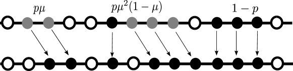
Figure 1: Example of cluster updates in GTASEP. The gray particles in the starting configuration are those, which have decided to jump, and the black ones will stay. In the rightmost cluster all particles stay on their places with probability $1-p$, which is the probability for the first particle to stay, while the others stay with probability one. Three particles from the middle cluster jump with probabilities $p,\mu$ and $\mu$ and the last one stays with probability $1-\mu$. Both particles in the leftmost cluster jump with probabilities $p$ and $\mu$.

This dynamics is illustrated in fig. 1. Particular limiting cases of this dynamics corresponding to $\mu=0$ and $\mu=p$ are known as TASEP with parallel and backward sequential updates respectively rajewsky1998asymmetric . In the former, at each time step all particles are updated simultaneously, having the same probability $p$ of jump to the right, provided that the right neighboring site in the current configuration is empty. In the latter they also jump to the right with the same probability $p$ being updated sequentially from right to left. The fact that GTASEP interpolates between the two updates is responsible for the coined term generalized update.

One can summarize the update of each cluster saying that the transition

$$(0,1^{(k)},0)\to(0,1^{(k-l)},0,1^{(l)})$$

occurs with probability $\varphi(l|k)$ defined by

$$\varphi(l|k) = p\mu^{l-1}(1-\mu),\,\,\,\mathrm{for\,\,\,}0<l<k$$

$$\varphi(0|k) = (1-p),\,\,\,\,\,\,\,\,\,\,\,\,\,\,\,\,\,\,\,\,\,\,\,\,\,\,\,\,0<k$$ (1)

$$\varphi(k|k) = p\mu^{k-1},\,\,\,\,\,\,\,\,\,\,\,\,\,\,\,\,\,\,\,\,\,\,\,\,\,\,\,\,\,\,0<k$$

for every cluster independently. One may recognize in these formulas the $q=0$ limit of the jumping probabilities of three-parametric integrable chipping model P2013 also known as q-Hahn boson model BCPS2013 . That model is defined as a system of particles on a one-dimensional lattice with zero-range type interaction. Configurations $\mathbf{n}=\{n_{i}\}_{i\in\mathbb{Z}}$ of the model are also defined in terms of the numbers of particles at each site, which now can take any value $n_{i}\geq 0$. The system evolves in discrete time. Within an update, given current configuration $\mathbf{n}$, we draw the number $0\leq m_{i}\leq n_{i}$ of particles to jump from every site $i\in\mathbb{Z}$ from the probability distribution $\varphi(m_{i}|n_{i})$ independently of the others. The exmples of updates are shown in fig. 2. The three-parametric family of distributions $\varphi(m|n)$ ensuring the Bethe ansatz solvability of the model was obtained in P2013 in the form

$$\varphi(m|n)=\mu^{m}\frac{(\nu/\mu;q)_{m}(\mu;q)_{n-m}}{(\nu;q)_{n}}\frac{(q;q)_{n}}{(q;q)_{m}(q;q)_{n-m}},$$ (2)

where $\mu,\nu$ and $q$ are real parameters to be chosen such that that $\varphi(m|n)$ is a probability distribution, and $(a;q)_{n}=(1-a)\dots(1-aq^{n-1})$ is the q-Pochhammer symbol.

Figure 2: An update of the q-Hahn boson model and of the associated model with exclusion interaction obtained via the ZRP-ASEP mapping. In the q-Hahn boson model $m$ particles jump to the next site on the right from a site with $n\geq m$ particles with probability $\varphi(m|n)$. Particles having decided to jump are shown in gray color. Under the ZRP-ASEP mapping a site with $n$ particles is replaced by a cluster of $n$ one-particle sites plus one empty site on the right. A jump of $m$ particles from a site in the q-Hahn boson model corresponds to the shift of the rightmost $m$-particle piece of the corresponding cluster one step to the right.

One can check that the $q=0$ limit of (2) coincides with (1) if one sets

$$\nu=\frac{\mu-p}{1-p}.$$

To see that the two models are tightly related we establish a connection between the zero-range process (ZRP), where the occupation numbers are unbounded, and the ASEP-like system with at most one particle in a site referred to as ZRP-ASEP mapping in P2013 . To this end, we replace a site with $n$ particles in the ZRP-like system by the sequence of $n$ sites with one particle in each plus one empty site on the right, see fig. 2. The correspondence between evolutions of these two systems is then one-to-one.

Taking the $q=0$ limit leads to a crucial simplification of the model. In this case it acquires the structure of a determinantal process, which makes the calculation of all finite-dimensional distributions of particle positions possible. The results on the distribution for two cases of IC are given in the next subsection.

2.2 Finite-dimensional distributions: exact formulas

Here we present exact formulas for joint distributions of positions of tagged particles at fixed time $t$, given initially the particles either densely occupied the negative half of the lattice

$$\eta(0)=\eta_{\mathrm{step}}:=\left\{\eta_{i}=\mathbbm{1}_{i<0}\right\}_{i\in\mathbb{Z}}$$

or every second site of the whole lattice

$$\eta(0)=\eta_{\text{alt}}:=\left\{\eta_{i}=\mathbbm{1}_{i\in 2\mathbb{Z}}\right\}_{i\in\mathbb{Z}}.$$

As usual, these two configurations are referred to as step and alternating IC, respectively. To keep track of particles’ history we assign every particle with an integer index $n$ and denote the position of particles at time $t$ by $x_{n}(t)$, assuming that initially

$$x_{n}(0) =-n,\,\,n\in\mathbb{Z}_{>0}$$

for step initial conditions, and

$$x_{n}(0)=-2n,\,\,n\in\mathbb{Z}$$

for alternating IC.

A simpler problem of description of the GTASEP evolution of a finite particle configuration was solved in gtasep . There, the Green function, i.e. the joint distribution of positions of all particles given an arbitrary initial $N$-particle configuration was obtained in form of the determinant of $N\times N$ matrix. The following result based on that result, however, addresses the evolution of infinite particle configurations. An infinite-dimensional random process can be described by specifying the complete set of finite dimensional distributions, associated in general with arbitrary sets of time points. Below we provide the formulas for purely spacial multipoint distributions, aka the distributions of positions of finite subsets of particles associated with the fixed moment of time.

The finite dimensional distributions will have the form similar to that obtained earlier for several other models of this type. Specifically, the $m$-point distribution will be given by the Fredholm determinant of an operator acting on functions on the set $\mathbb{Z}\times(1,\dots,m)$, i.e. the the disjoint union of $m$ copies of the set $\mathbb{Z}$, where particle coordinates live. Let the action of the operator, say denoted by $K$, on functions

$$(Kf)(n,x)=\sum_{i=1}^{m}\sum_{y\in\mathbb{Z}}K(n,x;i,y)f(i,y)$$ (3)

be defined in terms of a matrix kernel $K(n,x;i,y)$. Then, the Fredhom determinant can be represented as series

$$\det(1-K)_{\ell^{2}\left(\{1,\dots,m\}\times\mathbb{Z}\right)}$$ (4)

$$:=\sum_{k=0}^{\infty}\frac{(-1)^{k}}{k!}\sum_{i_{1},\dots,i_{k}=1}^{m}\sum_{x_{i_{1}},\dots,x_{i_{k}}\in\mathbb{Z}}\det\{K(i_{l},x_{i_{l}},i_{s},x_{i_{s}})\}_{1\leq s,l\leq k}.$$

Though, other more abstract definitions of the Fredhom determinant exist, it is the definition (4) referring only to the form of the kernel that will be exploited in the present paper.

Theorem 2.1

Consider $m$ particles with indices $n_{1}<\dots<n_{m}$ evolving under GTASEP conditioned to an (infinite) initial configuration $\eta(0)$, which can be either $\eta_{step}$ or $\eta_{alt}$. The joint probability for their positions $x_{n_{1}}(t)>\dots>x_{n_{m}}(t)$ to take values in half-axes $(x_{n_{1}}\geq a_{1},\dots,x_{n_{m}}\geq a_{m})$ is given by Fredholm determinant

$$\mathbbm{P}\Big{(}\bigcap_{k=1}^{m}\big{\{}x_{n_{k}}(t)\geq a_{k}\big{\}}|\eta(0)\Big{)}=\det(\boldsymbol{1}-\bar{P}_{a}K_{t}\bar{P}_{a})_{\ell^{2}(\{1,\dots,m\}\times\mathbbm{Z})}$$ (5)

of the operator $\bar{P}_{a}K_{t}\bar{P}_{a}$ with the $m\times m$ matrix kernel

$$K(k,x;l,y)=\bar{P}_{a}(k,x)K_{t}(n_{k},x;n_{l},y)\bar{P}_{a}(l,y),\quad 1\leq k,l\leq m,$$

composed of projectors

$$\bar{P}_{a}(n,x)=\mathbbm{1}_{x<a_{n}}$$ (6)

restricting the internal summations in (3,4) to the complementary half-axes and the kernel of the operator $K_{t}$ of the form

$$K_{t}(n_{k},x;n_{l},y)=-\phi^{*(n_{k},n_{l})}(x,y)+\widetilde{K}_{t}(n_{k},x;n_{l},y)$$ (7)

where

$$\phi^{*(n_{k},n_{l})}(x,y)=\mathbbold{1}_{n_{l}>n_{k}}\oint_{\Gamma_{1}}\frac{dv}{2\pi\mathrm{i}}\frac{(\nu-1)(1-v)^{n_{l}+y-n_{k}-x-1}}{v^{n_{l}-n_{k}}(1-\nu v)^{n_{l}+y-n_{k}-x+1}}$$ (8)

and $\widetilde{K}_{t}(n_{k},x;n_{l},y)$ is either

$$\!\!\!\!\widetilde{K}_{t}^{step}(n_{k},x;n_{l},y)$$

$$\!\!\!\!\!\!\!\!\!\!\!\!\!\!\!\!\!\!\!\!\!\!\!\!\!\!\!\!\!\!\!\!\!\!\!\!\!\!\!\!\!\!\!\!\!=\oint_{\Gamma_{1}}\frac{du}{2\pi\mathrm{i}}\oint_{\Gamma_{0}}\frac{dv}{2\pi\mathrm{i}}\frac{u^{n_{k}}(1-\mu u)^{t}(1-v)^{y+n_{l}}(1-\nu u)^{n_{k}+x-t-1}}{v^{n_{l}}(1-\mu v)^{t}(1-u)^{x+n_{k}+1}(1-\nu v)^{n_{l}+y-t}}\frac{(1-\nu)}{(v-u)}$$ (9)

or

$$\widetilde{K}_{t}^{alt}(n_{k},x;n_{l},y) =\oint_{\Gamma_{0}}\frac{dv}{2\pi\mathrm{i}}\frac{(1-v)^{y+n_{l}+n_{k}}(1-p+vp)^{t}}{v^{x+n_{k}+n_{l}+1}(1-\mu v)^{t}(1-\nu v)^{y+n_{l}+n_{k}-t}}$$ (10)

for step and alternating IC respectively. Here $\Gamma_{0}$ (resp $\Gamma_{1}$) is any simple loop, anticlockwise oriented, which encloses the only pole $v=0$ $(v=1)$ and no any other poles of the integrand.

Formulas (8) and (9) of the kernel for step IC were first obtained in KnizelPetrovSaenz .

2.3 Scaling limits

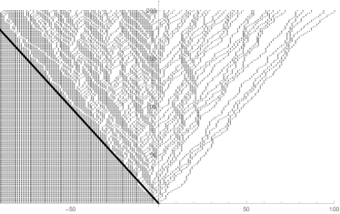
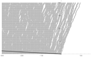
(a)                                                          (b)

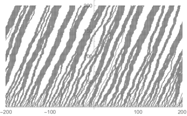
(c)                                                          (d)

Figure 3: The 200 steps samples of evolution of GTASEP with step, (a) and (b), and alternating, (c) and (d), initial conditions corresponding to KPZ and transitional regimes respectively. Space and time coordinates are displayed on the horizontal and vertical axes respectively. The values of parameters are $\mu=0$ in (a),(c) and $\mu=0.99$ in (b),(d) and $p=0.5$ in all cases. The black line in step IC plots (a) and (b) is the left border of the rarefaction fan.

Though the finite dimensional distributions contain complete information about the process, the above results are of limited scope, being of complicated form, specific for the particular model only. They acquire a general meaning in scaling limits, when we zoom out the system to time and space scales in which the microscopic details are not important and the universal features specific for large classes of systems remain.

Below we consider two different scaling limits of the exact formulas corresponding to two types of behavior illustrated by fig.3, which we refer to as KPZ and transitional regimes. The KPZ regime is observed in the large time limit $t\to\infty$ at generic values of the parameters of the model, $0<p<1$ and $0\leq\mu<1$. In this case GTASEP represents a typical driven-diffusive system with short-range interactions subject to an uncorrelated random force, which is generally believed to belong to the KPZ universality class. The transitional regime is associated with the simultaneous limits $\mu\to 1$ and $t\to\infty$ competing for the choice between the KPZ regime and the DA limit, in which particles irreversibly merge into growing clusters moving diffusively.

Technically the limits will be obtained from the asymptotic analysis of the exact formulas. However, before going to exact statements let us discuss how the scaling limits are expected to look like on a heuristic level. In particular, in the KPZ part we introduce all the model-dependent constants that will then be used in the statement of the theorem 2.2 and explain how they naturally appear from the quasi-equilibrium hypothesis as the characteristics of the translation invariant stationary state of the infinite system. Also, we explain the physical reasoning behind the choice of the mutual scaling of $t$ and $(1-\mu)$ that will be used in theorem 2.3 for the transitional regime.

2.3.1 KPZ scaling

In the KPZ regime the distance traveled by a particle in the bulk of the system consists of the deterministic $O(t)$ part and of the random fluctuations on the scale $O(t^{1/3})$. In a mathematically rigorous sense the convergence of random variables like $x_{n}(t)/t$ to non-random ones, known as the law of large numbers (LLN), is widely believed and proved for some models to hold almost surely Rost , Pablo_Ferrari . Heuristically, the value of the limit follows from the hypothesis of local quasi-equilibrium meaning that from the large scale perspective particles are carried by the particle flow, which locally behaves in the same way as the one in the stationary state of the infinite translationally invariant system. The only function responsible for everything taking place in the hydrodynamic (i.e. of order of $t$) scale is the particle current $j_{\infty}(c)$ maintained by such a system at particle density $c$.

For example, in a system with constant particle density $c$ a particle moves with constant velocity, $x_{n}(t)-x_{n}(0)=v(c)t$, where the particle velocity $v(c)$ is related to the current by $v(c)=j_{\infty}(c)/c$. It is the case for the alternating IC corresponding to $c=1/2$. In the non-stationary setting of step IC the particles move in the varying density profile described by the Euler hydrodynamics governed by the particle conservation law. We refer the reader to appendix A.1, were we explain that in the large time limit, $t\to\infty$, the coordinate of a particle with number $n=\theta t$ is given by $x_{n}\simeq t\chi(\theta),$ where the function $\chi(\theta)$ is an inversion of the function $\theta(\chi)$ obtained as a Legandre transform

$$\theta=\inf_{c\in[0,1]}(j_{\infty}(c)-c\chi)$$ (11)

of the function $j_{\infty}(c)$ assumed to be convex.

Thus, having the function $j_{\infty}(c)$ as an input the hydrodynamics fixes the linear in time deterministic part of $x_{n}(t)$ corresponding to LLN. The random part is the KPZ analogue of the central limit theorem. The KPZ universality suggests that the random fluctuations of order of $O(t^{1/3})$ are non-trivially correlated between the spacial positions within the scale $O(t^{2/3})$. Hence, choosing the number $n$ of a particle in $O(t^{2/3})$ vicinity of some macroscopic reference value $t\theta$,

$$n=t\theta+t^{2/3}\kappa_{c}u$$ (12)

we expect that the distance traveled by a particle will have the form

$$x_{n}(t)\simeq x_{n}(0)+tj_{\infty}(c)/c+\kappa_{f}\mathcal{X}_{flat}(u)t^{1/3},$$ (13)

for flat IC and

$$x_{n}(t)\simeq t\chi(\theta)+\kappa_{f}\mathcal{X}_{step}(u)t^{1/3},$$ (14)

for step IC with $\chi(\theta)$ being the inverse of (11). The scaling factors $\kappa_{f}=\kappa_{f}(c)$ and $\kappa_{c}=\kappa_{c}(c)$ are model-dependent parameters to be defined below, aka units in the fluctuation and correlation scales respectively depending on particle density $c$, the parameter $u$ is the scaled particle number relative to the macroscopic reference value $t\theta$ and $\mathcal{X}_{flat}(u),\mathcal{X}_{step}(u)$ are families of correlated random variables parameterized by $u$, i.e. random processes expected to be universal within the KPZ universality class for the same large scale shapes of initial conditions. In the spirit of local quasi-equilibrium $\kappa_{f}$ and $\kappa_{c}$ are functions of $\theta$ in the case of step IC, since the density $c=c(\chi)$ depends on the scaled coordinate $\chi=\chi(\theta)$, which is in turn related with $\theta$ by (11). That the model dependent scaling factors have the same form in the two cases is another demonstration of the KPZ universality.

The conjectures (13,14) for the distances traveled by particles are formulated in terms of yet unknown functions $j_{\infty}(c),\chi(c),\kappa_{f}(c)$ and the function $\chi(\theta)$ related with $j_{\infty}(c)$ via (11). They will be derived in course of the asymptotic analysis of the exact distributions. In this way, the functions appear as a result of technical calculations, while their physical meaning remain beyond our scope. At the same time, these quantities can be given a transparent interpretation in the spirit of the local quasi-equilibrium by expressing them in terms of observables of the translation invariant stationary state in the infinite system. We sketch the argument here, while the details of calculations are moved to appendix sections A.2,A.3.

Instead of considering the GTASEP, it is simpler to deal with the equivalent ZRP-like system described above. There is a one-parametric family of transitionally invariant stationary measures in such systems, which are product measures, see e.g. Woelki ; DPP2015 . Specifically the numbers of particles $n_{i},i\in\mathbb{Z},$  are identically distributed independent random variables with one-site distribution

$$\mathbb{P}(n_{i}=k)=\frac{f(k)z_{c}^{k}}{\mathfrak{z}(z_{c})}$$ (15)

parameterized by a single parameter $0\leq z_{c}\leq 1$ called the particle fugacity. Here $f(k)=\delta_{k,0}+(1-\delta_{k,0})(1-\nu)$ is the one site weight and $\mathfrak{z}(z_{c})$ is the normalization factor or one-site partition function. The particle density and current in such a system can be calculated as corresponding averages

$$\rho=\mathbb{E}n_{i},\quad j_{\infty}^{ZRP}=\mathbb{E}\sum_{m=0}^{n_{i}}m\varphi(m|n_{i}).$$

while for their counterparts in the ASEP-like system we obtain $c=\rho/(1+\rho)$ and $j_{\infty}=j_{\infty}^{ZRP}(1-c)$. In terms of $z_{c}$ they take the following form

$$c = \frac{(1-\nu)z_{c}}{\nu z_{c}^{2}-2\nu z_{c}+1},$$ (16)

$$j_{\infty} = \frac{(\mu-\nu)\left(1-z_{c}\right)z_{c}}{\left(1-\mu z_{c}\right)\left(1-\nu\left(2-z_{c}\right)z_{c}\right)},$$ (17)

which used with (218,11) yeilds

$$\chi = \frac{(\mu-\nu)(1-2z_{c}+z_{c}^{2}(\mu+\nu-2\mu\nu)-\mu\nu z_{c}^{4}+2\mu\nu z_{c}^{3})}{(1-\nu)(1-\mu z_{c})^{2}(1-\nu z_{c}^{2})},$$ (18)

$$\theta = \frac{(\mu-\nu)(1-\mu)z_{c}^{2}}{(1-\mu z_{c})^{2}(1-\nu z_{c}^{2})}.$$ (19)

       

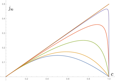
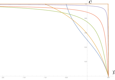
(a)                                                           (b)

Figure 4: Current-density diagrams $j_{\infty}(c)$ (a) and particle density profiles $c(\chi)$ (b) for $p=1/2$ and different values of $\mu$. Going from bottom to top the plots correspond to $\mu=0,0.5,0.9,0.99,0.9999,1.$

In appendix section A.2 we prepare the stationary state of the GTASEP in the infinite system starting from that on the finite ring and then taking the thermodynamic limit. There, the parameter $z_{c}$ naturally appears as a saddle point of the integrand within the integral represenation of the stationary state averages. The latter approach also allows calculation of the universal finite size correction to the current on the ring used in construction of the scaling factors $\kappa_{f},\kappa_{c}$. In section A.3, these quantities are expressed in terms of two dimensionful scaling invariants of the KPZ theory using the dimensional analysis and scaling hypothesis proposed in KM1990 ; amar1992universal ; KMH1992 . Connection of the dimensionful invariants with stationary state observables allows one to express $\kappa_{f}$ and $\kappa_{c}$ in terms of $z_{c}$.

$$\kappa_{f} = \frac{\left[(1-\mu)(\mu-\nu)(1-\mu\nu z_{c}^{3})\right]^{1/3}\left[\left(1-\nu z_{c}\right)\left(1-z_{c}\right)\right]{}^{2/3}}{\left(1-\nu\right)\left(1-\mu z_{c}\right)\left[z_{c}(1-\nu z_{c}^{2})\right]^{1/3}}$$ (20)

$$\kappa_{c} = \frac{z_{c}^{4/3}\left[\left(1-\nu z_{c}\right)\left(1-z_{c}\right)\right]^{1/3}\left[(1-\mu)(\mu-\nu)\left(1-\mu\nu z_{c}^{3}\right)\right]^{2/3}}{\left(1-\mu z_{c}\right){}^{2}\left(1-\nu z_{c}^{2}\right){}^{5/3}}$$ (21)

The formulas (16-21) obtained heuristically will appear below from the rigorous steepest descent analysis of the integral formulas (8-10), where $z_{c}$ is the double saddle (critical) point of the integrand, hence the subscript. To obtain one of the quantities as a function of another, one has to eliminate $z_{c}$ between the pair of equations. An example is the function $j_{\infty}(c)$ first appeared in Woelki . Obtained by resolving the quadratic equation (16) with respect to $z_{c}$ and substituting the result into (17) it has relatively simple form, while the other functions, like e.g. $c(\chi)$, are more complex involving the roots of polynomials of higher degrees. On the other hand the parametric form (16-21) turns out to be more convenient to work with. In particular this is the form these quantities arising from the steepest descent analysis below.

In fig. 4 we plot the current-density diagrams, $j_{\infty}(c)$, and the density profiles, $c(\chi)$, for different values of $\mu$. One can see that as $\mu$ approaches one, the first graph tends to the linear plot $j_{\infty}=pc$ and the second one becomes the step function $c=\mathbbm{1}(\chi<p)$. This limit is the subject of the following discussion.

2.3.2 Transitional scaling

The closer $\mu$ is to one, the more effort particles make to take over the particles ahead making the typical particle cluster in the system longer. In the DA limit, which we define as the limit $\mu\to 1$ as $p<1$ is kept constant, the clusters irreversibly merge into bigger clusters, each moving as a single particle. In particular, they move diffusively, i.e. in the limit $t\to\infty$ the fluctuations of traveled distance $x_{n}(t)$ measured in the diffusive scale are Gaussian, $x_{n}(t)\simeq pt+\left(\Delta t\right)^{1/2}\mathcal{N},$ where $\mathcal{N}$ is the standard normal random variable. The signature of the diffusive behavior is a non-zero diffusion coefficient, which is $\Delta=p(1-p)$ for a single particle.

It was shown in DPP2015 for the case of periodic system that these two types of universal behavior are connected by the transitional regime. It takes place when the parameter

$$\lambda=\frac{1}{1-\nu},$$

which diverges to infinity as $\mu\to 1$ while $p$ is fixed, scales as $L^{2}$, the size of the system squared. When the crossover parameter $\lambda/L^{2}$ varies from zero to infinity, the average number of particle clusters on the lattice gradually decreases from infinity to one and the statistics of particle current, specifically the functional form of LDF of the distance traveled by particle (measured in the diffusive scale), changes from the KPZ to purely Gaussian form.

To guess the scaling in the non-stationary setting we adopt the quasi-equilibrium hypothesis to the system of large particle clusters. Since a cluster of particles in GTASEP corresponds to an occupied site with occupation number distributed according to (15), the cluster length $l_{cl}$ is a geometric random variable with distribution

$$\mathbb{P}(l_{cl}=k)=z_{c}^{k-1}(1-z_{c}),k\in\mathbb{N}.$$

In particular, the mean cluster size is $\left\langle l_{cl}\right\rangle=(1-z_{c})^{-1}$. At large $\lambda$ and fixed density $c$, related with $z_{c}$ by (16), it is estimated to

$$\left\langle l_{cl}\right\rangle=(1-z_{c})^{-1}\simeq\sqrt{c\lambda/(1-c)}.$$

We also estimate the average gap between clusters to be $\left\langle l_{cl}\right\rangle(1/c-1)$ by noting that the average distance per one cluster is $\left\langle l_{cl}\right\rangle/c$ and the fraction of empty sites within this distance is $(1-c)$.

Then for the transitional regime we expect that

– the fluctuations of the distance traveled by a particle are diffusive,

$$\delta x_{n}(t)\varpropto\sqrt{p(1-p)t};$$ (22)

– for the time under consideration a cluster interacts with finitely many clusters, i.e. fluctuations of the traveled distance is of order of the typical gap between clusters

$$\sqrt{tp(1-p)}\varpropto\sqrt{\lambda(1-c)/c};$$ (23)

– particles are correlated, when they are a finite number of clusters apart, i.e. the particle number $n$ should be measured in the units of average cluster length,

$$\delta n\varpropto\left\langle l_{cl}\right\rangle.$$ (24)

Thus, when the particle density is fixed away from zero and one, i.e. the clusters and gaps between them are of comparable size, both the correlation and fluctuation scales are of order of $O(\sqrt{\lambda})$, while $\lambda\varpropto t$. This is the case for the alternating IC.

For step IC the density ranges from zero to one, and we can also probe into the situations, in which the density is in the vicinity of the ends of its range. To this end, we consider a family of scalings parameterized by a parameter $\beta\in(0,1)$ setting $z_{c}=1-O(\lambda^{-\beta})$, which generalizes the above $z_{c}=1-O(1/\sqrt{\lambda})$. Practically, this means that the average cluster length is $\langle l_{cl}\rangle=O(\lambda^{\beta})$ and the gap length scales as $O(\lambda^{1-\beta})$. The length of the region containing finitely many rightmost clusters is dominated either by clusters or by gaps corresponding to the densities $c=1-O(\lambda^{1-2\beta})$ or $c=O(\lambda^{2\beta-1})$, when $1/2<\beta<1$ or $0<\beta<1/2$ respectively. Then, the scaling $\lambda^{1-\beta}\varpropto\sqrt{t}$ as well as the correlation and fluctuation scales $\delta x_{n}(r)\varpropto\lambda^{1-\beta},\delta n\varpropto\lambda^{\beta}$ follow from the formulas (22-24).

To summarize, we expect that the transitional regime is associated with a double limit $t,\lambda\to\infty$, such that the ratio $\lambda^{1-\beta}/\sqrt{t}$ is kept constant. Taking $n=[r\lambda^{\beta}]$ with $r$ fixed we expect that the distance traveled by the particle with number $n$ will be

$$x_{n}(t)-x_{n}(0)\simeq pt+\sqrt{p(1-p)t}\mathcal{X}(r),$$ (25)

where $\mathcal{X}(r)$ is the random process expected be universal for a given global shape of initial conditions. In our cases, $\beta=1/2$ should be taken for the alternating IC, while for the step IC the whole range $0<\beta<1$ is meaningful.

It will be convenient to introduce the crossover parameter

$$\tau_{\beta}=\frac{\sqrt{tp(1-p)}}{\lambda^{1-\beta}}.$$

that controls the crossover between the KPZ regime and the DA limit. As $\tau_{\beta}$ increases the number of clusters involved into the evolution grows to infinity, returning us to the KPZ regime. In the opposite situation $\tau_{\beta}\to 0$ the system approaches the DA limit, in which $\mathcal{X}(r)$ is expected to be Gaussian and $r$-independent, since all particles move synchronously as a single particle in this case. The coefficient of the random part in (25) is chosen in such a way, that $\mathcal{X}(r)$ becomes the standard normal variable in the DA limit.

2.3.3 Limiting processes

Now we are in position to make rigorous statements about the limiting processes that appear under the scalings (13,14,25) and their relations with each other. The whole scheme is outlined in fig. 5. We obtain four main processes: $\mathcal{A}_{1}(u),\mathcal{A}_{2}(u)$ corresponding to Airy₁ and Airy₂ processes that appear in the KPZ regime for alternating and step IC respectively and $\mathcal{X}^{(\tau)}_{\mathcal{A}_{1}\to\mathcal{N}}$ and $\mathcal{X}_{\mathcal{A}_{2}\to\mathcal{N}}$ corresponding to the transitional regime for the same IC. Then, we perform further limits of the transitional processes towards the KPZ regime and the DA limit, yielding the fully correlated normal random variables.

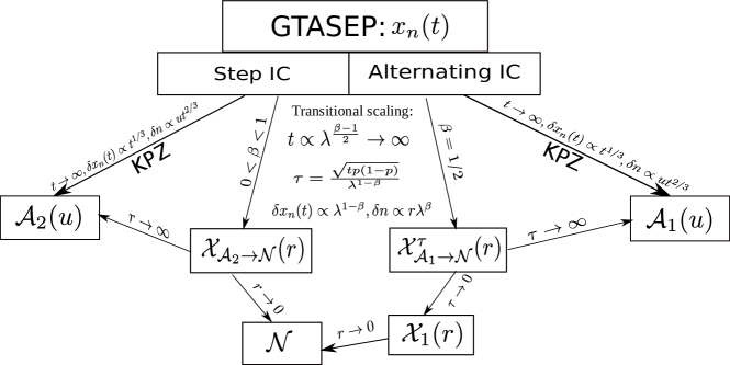
Figure 5: Limiting processes in GTASEP. The arrows show the directions of limiting transitions. We explicitly indicate the form of the scalings corresponding to the KPZ and transitional regimes in GTASEP. Further limits can be taken of the transitional processes $\mathcal{X}_{\mathcal{A}_{2}\to\mathcal{N}}$ and $\mathcal{X}_{\mathcal{A}_{1}^{\tau}\to\mathcal{N}}$, which finally either return them to the KPZ regime or bring them to the DA regime, where the processes collapse into a single normal random variable $\mathcal{N}$. We show these limits by arrows indicating in which parameter the limit is performed. The limit of $\mathcal{X}^{(\tau)}_{\mathcal{A}_{1}\to\mathcal{N}}$ towards DA is performed in two steps via an intermediate process $\mathcal{X}_{1}$.

The limiting processes are also characterized by their finite dimensional distributions obtained as limits of the exact distributions of theorem 2.1 and having the form of Fredholm determinants of specific operators. In the scaling limit the particle coordinates become continuous and the operators involved into definitions of the $m$-point distributions act on functions on the disjoint union of $m$ copies of $\mathbb{R}$, i.e. on the set isomorphic to $\{1,\dots,m\}\times\mathbb{R}$. The action of the operator, say $K$ again, on functions

$$(Kf)(n,x)=\sum_{i=1}^{m}\int_{\mathbb{R}}K(n,x;i,y)f(i,y)dy$$ (26)

is defined in terms of kernel $K(n,x;i,y)$, which is also used to represent the Fredhom determinant in the form of infinite series.

$$\det\left(\boldsymbol{1}-K\right)_{L^{2}((1,\dots,m)\times\mathbb{R})}$$ (27)

$$=\sum_{k=1}^{\infty}\frac{(-1)^{k}}{k!}\sum_{i_{1},\dots,i_{k}=1}^{m}\int_{\mathbb{R}^{k}}\det\left\{K(i_{j},x_{j};i_{l},x_{l})\right\}_{j,l=1}^{m}d^{k}x.$$

In the present paper we deal with two universal processes referred to as Airy₁ and Airy₂ processes, corresponding to the step and flat IC respectively.

Definition 1

The Airy₁ and Airy₂ processes are the random processes $\mathcal{A}_{1}:\mathbb{R}\to\mathbb{R}$ and $\mathcal{A}_{2}:\mathbb{R}\to\mathbb{R}$, respectively, defined by their finite dimensional distributions. For any $m\in\mathbb{N}$, any $m$-point sets $r=$ ($r_{1},\dots,r_{m})\subset\mathbb{R}$ and $(a_{1},\dots,a_{m})\subset\mathbb{R}$ the joint distribution of values of $(\mathcal{X}(r_{1}),\dots\mathcal{X}(r_{m}))$ with either $\mathcal{X}=\mathcal{A}_{1}$ or $\mathcal{X}=\mathcal{A}_{2}$ is given by the Fredhom determinant

$$\mathbb{P}\left(\bigcap_{k=1}^{m}\left(\mathcal{X}(r_{k})<a_{k}\right)\right)=\det\left(\boldsymbol{1}-P_{a}K_{\mathcal{X}}P_{a}\right)_{L^{2}(\{1,\dots,m\}\times\mathbb{R})}$$ (28)

of the operator $P_{a}K_{\mathcal{X}}P_{a}$ with $m\times m$ matrix kernel

$$K(i,x;j,y)=P_{a}(i,x)K_{\mathcal{X}}(r_{i},x;r_{j},y)P_{a}(j,y),\quad 1\leq i,j\leq m$$

composed of projectors

$$P_{a}(k,x)=\mathbbm{1}_{x\geq a_{k}},\quad k=1,\dots,m$$ (29)

and the kernel of an integral operator $K_{\mathcal{X}}$ being one of the kernels

$$K_{\mathcal{A}_{1}}(r_{i},x;r_{j},y) = -\frac{\mathbbold{1}_{r_{j}>r_{i}}}{\sqrt{4\pi(r_{j}-r_{i})}}\exp\left(-\frac{(y-x)^{2}}{4(r_{j}-r_{i})}\right)$$

$$\!\!\!\!\!\!\!\!\!\!\!\!\!\!\!\!\!\!\!\!\!\!\!\!\!\!\!\!\!\!\!\!\!\!\!\!\!\!\!\!\!\!+\,\mathrm{Ai}\left((r_{j}-r_{i})^{2}+(y+x)\right)\exp\left(\frac{2}{3}(r_{j}-r_{i})^{3}+(r_{j}-r_{i})(y+x)\right),$$

or

$$\!\!K_{\mathcal{A}_{2}}(r_{j},x;r_{i},y) =\left\{\begin{array}[]{ll}\int_{0}^{\infty}d\xi e^{\xi(r_{j}-r_{i})}\mathrm{Ai}(\xi+x)\mathrm{Ai}(\xi+y),&r_{i}\geq r_{j}\\ -\int_{-\infty}^{0}d\xi e^{\xi(r_{j}-r_{i})}\mathrm{Ai}(\xi+x)\mathrm{Ai}(\xi+y),&r_{i}<r_{j}\end{array}\right..$$ (33)

respectively. Here $\mathrm{Ai}(z)$ is the Airy function that can be defined via its integral representation

$$\mathrm{Ai}(z)=\frac{1}{2\pi\mathrm{i}}\int_{\infty e^{-\mathrm{i}\phi}}^{\infty e^{\mathrm{i}\phi}}\exp\left({\frac{t^{3}}{3}-zt}\right)dt$$ (34)

as an integral along the contour composed of two rays outgoing from the origin at angles $\pm\phi$ to the real axis, where $\phi$ can be chosen in the range $\phi\in(\pi/6,\pi/2)$ and most often is taken to be $\phi=\pi/3$, which ensures the most rapid convergence. This is the definition that will be used below.

With these definitions in hand we are in position to make statements about the KPZ scaling limit of particle positions.

Theorem 2.2

Let $x_{n}^{\eta_{step}}(t)$ and $x_{n}^{\eta_{alt}}(t)$ be the position of a particle with number $n$ conditioned to step and alternating IC respectively. We define the functions $j_{\infty}(c),\kappa_{f}(c),\kappa_{c}(c),c(\chi)$ and $\chi(\theta)$ as the unique solution of parametric equations (16-21) obtained by eliminating the parameter $z_{c}$ varying in the range $z_{c}\in(0,1)$. Then, as $t\to\infty$ the following limits hold in a sense of finite dimensional distributions.

Step IC: KnizelPetrovSaenz

$$-\lim_{t\to\infty}\frac{x_{n}^{\eta_{step}}(t)-t\chi(\theta_{u})}{t^{1/3}\kappa_{f}(c(\chi(\theta)))}= \mathcal{A}_{2}(u),$$

where

$$n=t\theta_{u}:=t\theta+2t{}^{2/3}\kappa_{c}(c(\chi(\theta)))u,$$

the value of $\theta>0$ is such that $j^{\prime}_{\infty}(0)>\chi(\theta)\geq j^{\prime}(1)$.

Alternating IC:

$$-\lim_{t\to\infty}\frac{x_{n}^{\eta_{alt}}(t)+2n-2tj_{\infty}(1/2)}{(2t)^{1/3}\kappa_{f}(1/2)}=\mathcal{A}_{1}(u),$$

where

$$n=t\theta+2(2t)^{2/3}\kappa_{c}(1/2)u.$$

Remark 1

The powers of $2^{1/3}$ appearing in the coefficients is a normalization necessary to make the definitions of $\kappa_{f}(c)$ and $\kappa_{c}(c)$ given below consistent with the above definitions of universal Airy processes. This normalization is expected to be universal for interacting particle systems, provided that the scaling constants are related to the stationary state observables in the way to be specified in the next section.

The transitional processes are defined as follows.

Definition 2

Transitional processes $\mathcal{X}_{\mathcal{A}_{2}\to\mathcal{N}}:\mathbb{R}_{\geq 0}\to\mathbb{R}$ and $\mathcal{X}_{\mathcal{A}_{1}\to\mathcal{N}}^{(\tau)}:\mathbb{R}\to\mathbb{R}$ are defined by their finite dimensional distributions. Let us fix any $m\in\mathbb{N}$ and an $m$-point subset $r=\{r_{1},\dots,r_{m}\}$ of $\mathbb{R}_{\geq 0}$ or $\mathbb{R}$ for the first or the second case respectively. Then the multi-point distributions of the transitional processes are given by the Fredholm determinant formula (28) with either $\mathcal{X}=\mathcal{X}_{\mathcal{A}_{2}\to\mathcal{N}}$ or $\mathcal{X}=\mathcal{X}_{\mathcal{A}_{1}\to\mathcal{N}}^{(\tau)}$ and the kernel of $K_{\mathcal{X}}$ being

$$K_{\mathcal{A}_{2}\to\mathcal{N}}(r_{i},s_{1};r_{j},s_{2})$$ (35)

$$\!\!\!\!\!\!\!\!\!\!\!\!\!\!\!\!\!\!\!\!\!\!\!\!\!\!\!\!\!\!\!\!\!\!\!\!\!\!\!\!\!=\frac{1}{4\pi^{2}}\int_{\Gamma_{(-\mathrm{i}\infty,0^{-},\mathrm{i}\infty)}\!\!\!\!\!\!\!\!\!\!\!}dx_{1}\oint_{\Gamma_{0}}dx_{2}\frac{x_{1}\exp\left(\frac{x_{1}^{2}-x_{2}^{2}}{2}+\frac{r_{i}}{x_{1}}+s_{1}x_{1}-\frac{r_{j}}{x_{2}}-s_{2}x_{2}\right)}{x_{2}(x_{1}-x_{2})}$$

$$\,\,\,\,\,\,\,\,\,\,\,\,\,\,\,\,\,\,-\mathbbold{1}_{r_{j}>r_{i}}\left[\mathbbold{1}_{s_{2}>s_{1}}\sqrt{\frac{r_{ji}}{s_{21}}}I_{1}(2\sqrt{s_{21}r_{ji}})+\delta(s_{21})\right]$$

or

$$K_{\mathcal{A}_{1}\to\mathcal{N}}^{(\tau)}(r_{i},s_{1};r_{j},s_{2})$$ (36)

$$\!\!\!\!\!\!\!\!\!\!\!\!\!\!\!\!\!\!\!\!\!\!\!\!\!\!\!\!\!\!\!\!\!\!\!\!\!\!\!\!\!\!\!\!\!\!=\tau\int_{\Gamma_{(-\mathrm{i}\infty,0^{-},\mathrm{i}\infty)}\!\!\!\!\!\!\!\!\!\!\!}\frac{dx}{2\pi\mathrm{i}}\exp\left[\tau^{2}\frac{x^{2}-x^{-2}}{2}+\tau\left(s_{1}x-s_{2}x^{-1}-r_{ji}(x+x^{-1})\right)\right]$$

$$\!\!\!\!\!\!\!\!\!\!\!\!\!\!\!\!\!\!\!\!\!\!\!\!\!\!-\mathbbold{1}_{r_{j}>r_{i}}\left[\delta(s_{21}+r_{ji})+\mathbbold{1}_{s_{21}+r_{ji}>0}\frac{\tau I_{1}\left(2\tau\sqrt{r_{ji}\left(r_{ji}+s_{21}\right)}\right)}{\sqrt{1+s_{21}/r_{ji}}}\right]\!\!,$$

respectively, where $1\leq i,j\leq m$ and for brevity we used the notations $r_{ji}=r_{j}-r_{i}$ and $s_{ji}=s_{j}-s_{i}$. Here, $I_{1}(x)$ is the modified Bessel function of the first kind defind by the integral

$$I_{n}(x)=\oint_{\Gamma_{0}}t^{-n-1}e^{(x/2)(t+1/t)},$$ (37)

and $\delta(x)$ is the Dirac delta function.The integration contour $\Gamma_{0}$ is a counterclockwise loop closed around the origin and the contour $\Gamma_{(-\mathrm{i}\infty,0^{-},\mathrm{i}\infty)}$ is parallel to the imaginary axis going from $-\mathrm{i}\infty$ to $\mathrm{i}\infty$ leaving the origin and $\Gamma_{0}$ on the right, Fig.6. We also explicitly emphasize that in this case the Fredholm determinant is understood as the Fredholm sum (27), convergence of which will be proved below. Apparently, the kernels shown can not be used to define the trace class operators, at least unless properly conjugated. The operator content of Fredholm determinants with these kernels is yet to be understood.

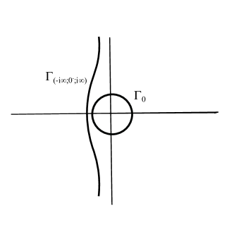
Figure 6: Integration contours

Note that the second kernel depends on the time variables only via difference parameter $r_{ji}$. Thus, $\mathcal{X}_{\mathcal{A}_{1}\to\mathcal{N}}^{(\tau)}(r)$ is stationary, while $\mathcal{X}_{\mathcal{A}_{2}\to\mathcal{N}}(r)$ is not. This is not unexpected as in the latter case the time parameter $r$ describes the coordinate along the variable density profile, while in the latter the density is constant.

Then, we can formulate the statements about the convergence of particle coordinates in the transitional regime.

Theorem 2.3

Consider simultaneous limits $t\to\infty,\lambda\to\infty$, such that $\tau_{\beta}=\lambda^{\beta-1}\sqrt{tp(1-p)}$, is constant. Then, for any $0<\beta<1$ and $\theta>0$ the limit

$$\lim_{t\to\infty}\frac{pt-\left(x_{[r\lambda^{\beta}]}^{\eta_{step}}(t)+r\lambda^{\beta}\right)}{\sqrt{tp(1-p)}}=\mathcal{X}_{\mathcal{A}_{2}\to\mathcal{N}}(\tau_{\beta}r),\,\,\,r\in\mathbb{R}_{\geq 0}$$

holds in the sense of finite dimensional distributions.

Also, for $\beta=1/2$ we have

$$\lim_{t\to\infty}\frac{pt-\left(x_{[r\sqrt{\lambda}]}^{\eta_{alt}}(t)+2r\sqrt{\lambda}\right)}{\sqrt{tp(1-p)}}=\mathcal{X}_{\mathcal{A}_{1}\to\mathcal{N}}^{(\tau_{1/2})}(r/\tau_{1/2}),\,\,\,r\in\mathbb{R}.$$

As was announced above, the processes obtained are expected to interpolate between the KPZ and DA regimes as $\tau_{\beta}$ varies in its range. For $\mathcal{X}_{\mathcal{A}_{2}\to\mathcal{N}}(r)$ this would be a statement about the behavior of the process at large and small values of the “time” parameter $r$ respectively, while for $\mathcal{X}_{\mathcal{A}_{1}\to\mathcal{N}}^{(\tau)}(r)$ we need to formulate the limits in terms of two parameters $\tau$ and $r$. As usual the ingredients of the KPZ part include the large scale deterministic part that should be extracted and the random part characterized by the fluctuation and correlation scales. The scales are supposed to be consistent with those of the KPZ regime described above after returning from $r$ and $\tau$ back to the variables of the original process. One can check that this is indeed the case in the limits below.

Proposition 1

KPZ tails:

Let $\mathcal{X}_{\mathcal{A}_{2}\to\mathcal{N}}(r)$ and $\mathcal{X}_{\mathcal{A}_{1}\to\mathcal{N}}^{(\tau)}(r)$ be the processes defined in Def. 2. The following limits hold in the sense of finite dimensional distributions.

$$\left(2/3\right)^{1/3}\left(2r\right)^{1/9}\left(\mathcal{X}_{\mathcal{A}_{2}\to\mathcal{N}}\left(r_{u}\right)-\frac{3}{2}\left(2r_{u}\right)^{1/3}\right)\underset{r\to\infty}{\longrightarrow}\mathcal{A}_{2}(u)-u^{2},$$ (38)

where $r_{u}:=r+u\left(2r\right)^{7/9}\left(\frac{3}{2}\right)^{2/3},$ and

$$\left(\frac{\tau}{3}\right)^{1/3}\left(\mathcal{X}_{\mathcal{A}_{1}\to\mathcal{N}}^{(\tau)}(u\,3^{2/3}\tau^{1/3})-\tau\right)\underset{\tau\to\infty}{\longrightarrow}\mathcal{A}_{1}(u).$$ (39)

In the DA limit we expect that all particles move diffusively along the same trajectory, that is to say that the random variables representing the limiting process at different times are identical and normally distributed. To attain the limit for $\mathcal{X}_{\mathcal{A}_{2}\to\mathcal{N}}(r)$, we rescale the time $r$ by a factor $\epsilon,$ which is sent to zero afterwards. As a result we indeed come to the process that is represented by a single normal random variable independent of “time” parameter. The situation is more delicate for $\mathcal{X}_{\mathcal{A}_{1}\to\mathcal{N}}^{(\tau)}(r)$ because of the extra parameter $\tau$. In this case we come to the limit in two steps. In the first step we perform the limit $\tau\to 0,$ that brings us to yet another random process $\mathcal{X}_{1}(r)$.

Definition 3

The random process $\mathcal{X}_{1}:\mathbb{R}_{\geq 0}\to\mathbb{R}$ is defined by its finite dimensional distributions given by the Fredhom determinant formula (28) with $\mathcal{X}(r)=\mathcal{X}_{1}(r)$ and the kernel defined by

$$K_{\mathcal{X}_{1}}(r_{i},s_{1};r_{j},s_{2})=\frac{e^{-\frac{1}{2}\left(s_{1}+r_{i}-r_{j}\right)^{2}}}{\sqrt{2\pi}}-\mathbbold{1}_{r_{j}>r_{i}}\delta(s_{21}+r_{ji}),1\leq i,j\leq m$$ (40)

The process $\mathcal{X}_{1}(r)$ has normal one-point distribution, while the multipoint distributions seem to be nontrivial, though have not been studied yet. The subsequent limit is taken in the same way as the one for $\mathcal{X}_{\mathcal{A}_{2}\to\mathcal{N}}(r)$, yielding the similar result. Note that as $\mathcal{X}_{\mathcal{A}_{1}\to\mathcal{N}}^{(\tau)}(r)$ is stationary the limits taken refer to the vicinity of an arbitrary point $r\in\mathbb{R}$, while the statement about $\mathcal{X}_{\mathcal{A}_{2}\to\mathcal{N}}(r)$ is the property of $r=0$ only.

Proposition 2

DA tails:

Let $\mathcal{X}_{\mathcal{A}_{2}\to\mathcal{N}}(r)$, $\mathcal{X}_{\mathcal{A}_{1}\to\mathcal{N}}^{(\tau)}(r)$ and $\mathcal{X}_{1}(r)$ be the processes defined in Defs. 2,3. The following limits hold in the sense of finite dimensional distributions

$$\mathcal{X}_{\mathcal{A}_{2}\to\mathcal{N}}(\epsilon r)\underset{\epsilon\to 0}{\longrightarrow}\mathcal{N},\quad r\in\mathbb{R}_{\geq 0},$$ (41)

$$\mathcal{X}_{\mathcal{A}_{1}\to\mathcal{N}}^{(\tau)}(r)\underset{\tau\to 0}{\longrightarrow}\mathcal{X}_{1}(r),\quad r\in\mathbb{R}$$ (42)

$$\mathcal{X}_{1}(\epsilon r)\underset{\epsilon\to 0}{\longrightarrow}\mathcal{N},\quad r\in\mathbb{R}$$ (43)

where $\mathcal{N}$ is the standard normal random variable that does not depend on $r$ anymore.

At the first glance the limits (41) and (43) look like the statement about the one-point distribution at one point $r=0$. We want to emphasize, however, that all the above limits are stated in terms of finite-dimensional distributions of all orders. The statement like this could be the consequence of the continuity of sample paths, if we had one a priori. Technically, the limits (41) and (43) follow from the convergence of the finite-dimensional distributions to those of the processes $\mathcal{X}_{\mathcal{N}}$ and $\mathcal{X}_{\mathcal{N},+}$ defined as follows.

Definition 4

The random processes $\mathcal{X}_{\mathcal{N},+}:\mathbb{R}_{\geq 0}\to\mathbb{R}$ and $\mathcal{X}_{\mathcal{N}}:\mathbb{R}\to\mathbb{R}$ are defined by their finite dimensional distributions given by the Fredhom determinant formula (28) with $\mathcal{X}=\mathcal{X}_{\mathcal{N},+}$ or $\mathcal{X}=\mathcal{X}_{\mathcal{N}}$ and the same kernel

$$K_{\mathcal{N}}(r_{i},s_{1};r_{j},s_{2})=\frac{\exp\left(-\frac{1}{2}s_{1}^{2}\right)}{\sqrt{2\pi}}-\mathbbm{1}_{r_{j}>r_{i}}\delta(s_{2}-s_{1}),1\leq i,j\leq m,$$ (44)

for both cases.

Then, statements (41) and (43) follow from the fact that the values of both processes at different points are trivially correlated each having the normal one-point distribution.

Proposition 3

Let $\mathcal{X}_{\mathcal{N},+}$ and $\mathcal{X}_{\mathcal{N}}$ be the random processes defined in Def. 4. For any $m\in\mathbb{N}$ and any $m$-point subset $r=(r_{1},\dots,r_{m})$ of either $\mathbb{R}_{\geq 0}$ or $\mathbb{R}$ for the former or the latter process respectively the identity

$$\mathcal{X}(r_{1})=\dots=\mathcal{X}(r_{m})$$ (45)

holds almost surely and

$$\mathcal{X}(r_{1})\sim\mathcal{N},$$ (46)

for both $\mathcal{X}=\mathcal{X}_{\mathcal{N},+}$ and $\mathcal{X}=\mathcal{X}_{\mathcal{N}}$.

The statement that the Fredholm determinant (28) with the kernel similar to (44) defines the joint distribution of trivially correlated random variables is a consequence of Prop. 4 proved in the end of this paper. The kernel (44) can be obtained as a limit from the kernel describing a particle obeying the Ornstein-Uhlenbeck process, which in turn was found in imamura2007dynamics as a limiting kernel for the tagged particle dominated by a defect particle in TASEP with slow particles, see formula (3.46) in imamura2007dynamics .

The kernel (35) that yields the distribution interpolating between the Tracy-Widom and normal distributions is to be compared with the kernel from baik2005phase appearing in the BBP distribution. Although they look different, there are similarities that make us wonder about possible connections between two transitions. Let us briefly discuss the resemblance with the example of the TASEP with step initial conditions and finitely many slower defect particles imamura2007dynamics . An effect of the defect particles is a formation of slow particle clusters, aka shock waves, each moving as a single particle, i.e. diffusively. As a result, similarly our findings fluctuations of the tagged particle can be either of KPZ type or Gaussian depending on whether the tagged particle is involved into the shock or not. The crossover between the two distributions is given by the BBP distribution. Its most general form corresponds to the case of the hopping rates of the defect particles being only slightly different from the non-defect ones with the difference measured on the scale $O(t^{-1/3})$. In this case the kernel of the Fredholm determinant defining the BBP distribution looks like the Airy kernel plus an additional finite rank part, with the rank equal to the number of defect particles. Equivalently it can be represented in an integral form similar to the one of the Airy kernel, but with as many additional poles in the integrand encoding the shifts. The poles disappear, when the hopping rates of the slow particles equalize with those of the rest of the system. In our case we also have different poles in the integrand within the initial exact kernel (9) owing to different hopping probabilities in our model. However, the order of these poles becomes infinite in the scaling limit and the merging of different poles leads to essential singularities in the integrand. It is likely that to obtain a similar behavior of the kernel in the system with slow particles one could possibly try to consider the number of slow particles growing to infinity, which scales together with vanishing difference between hopping rates of normal and defect particles. This scenario at least seems capable to produce singularities of similar type.

Also, when in the TASEP with slow defect particles all the hopping rates of the defect particles are distinct on the scale $O(1)$, only the slowest particle is relevant, and the BBP kernel degenerates to a simpler kernel appeared before in the studies of the polynuclear growth with sources imamura2004fluctuations ; imamura2005polynuclear . The one-point distribution defined as the Fredholm determinant with the latter kernel in turn interpolates between the so called GOE² baik2000limiting ; forrester2000painlev and Tracy-Widom distributions. It has a form of the Airy kernel plus a rank one part given by the product of Airy function and the integrated Airy function. Remarkably, by observing that $x_{1}/(x_{2}(x_{1}-x_{2}))=1/x_{2}+1/(x_{1}-x_{2})$ the double integral part of the kernel (35) can be split into infinite rank and rank one parts. These are the parts, which converge to the main parts of the Airy kernel (33) and of the Gaussian kernel (44) under the limits (38,41) respectively, while the other ones vanish. On the other hand, in the KPZ limit (38) the vanishing rank one part acquires the form of the product of Airy function and the integrated Airy function identical to that from the mentioned reduced BBP distribution imamura2007dynamics . The only difference with imamura2007dynamics is that this part is accompanied by a constant coefficient that makes the rank one part vanishingly small comparing to the Airy kernel. This may be an indication that our results have more in common with the BBP transition than we could find here. For example, it is an interesting question whether it is possible to find another scaling, under which the exact kernel (9) would again similarly converge to the sum of the Airy kernel and the rank one part described with the two being of the same order. We leave this question for further work.

It is also worth mentioning that the kernel of the form similar to (35) was obtained in kuijlaars2011non in studies of the double scaling limit of the non-intersecting Bessel paths. That kernel has an identical functional form with (35) up to the fact that the parameters responsible for the random variables and for the parameter of the process are interchanged. Whether this similarity is a pure coincidence or it has a deeper roots is also the matter for further investigation.

3 Determinantal point process and exact distributions

In this section we prove Theorem 2.1. The starting point is the determinant formula for Green function proved in gtasep . The Green function $G(X|Y;t)$ is the probability for particles of a finite configuration $\eta_{t}$ at time $t$ to have coordinates $X={x_{1}>x_{2}>\dots>x_{N}}$, given the coordinates $Y={y_{1}>y_{2}>\dots>y_{N}}$ of particles of initial configuration $\eta_{0}$.

Theorem 3.1

The Green function $G(X|Y;t)$ has a determinantal form

$$G(X|Y;t) = \lambda^{N(X)}\det(F_{i-j}(x_{N+1-i}-y_{N+1-j},t))_{1\leq i,j\leq N},$$ (47)

where $N(X)$ is the number of pairs of neighboring occupied sites in the final configuration $X$, and the functions $F_{n}(x,t)$ have integral representation

$$F_{n}(x,t) = (\nu-1)\oint_{\Gamma_{0,1}}\frac{du}{2\pi\mathrm{i}}\frac{(1-u)^{n-x-1}(1-\mu u)^{t}}{u^{n}(1-\nu u)^{n-x+t+1}}$$ (48)

where the integration contour $\Gamma_{0,1}$ is a simple loop counterclockwise oriented, which has the poles $u=0,1$ of the integrand inside and the others outside.

The key observation that allows a calculation of joint distributions of particle positions is that the Green function being a probability measure on the set of $N-$particle configurations is a marginal of a measure on a bigger space

$$\mathcal{D}=\{x_{i}^{n}\in\mathbb{Z},0\leq i\leq n\leq N|x_{i}^{n}>x_{i-1}^{n}\}$$

of configurations characterized by $\left(N+1\right)(N+2)/2$ coordinates, which turns out to be the determinantal process. To every $\boldsymbol{x}\in\mathcal{D}$ let us assign a measure

$$\mathcal{M}(\boldsymbol{x})=\mathrm{const}\bigg{(}\prod_{n=1}^{N-1}\det(\phi(x_{i}^{n},x_{j+1}^{n+1}))_{0\leq i,j\leq n}\bigg{)}\det\left(\Psi_{N-j}^{N}(x_{i}^{N})\right)_{1\leq i,j\leq N},$$ (49)

where we define the functions

$$\Psi_{j}^{N}(x):=F_{-j}(x-y_{N-j},t),\quad j=0,\dots,N-1$$ (50)

and

$$\phi(x,y):=\begin{cases}\nu-1,&y\geq x,\\ \nu,&y=x-1,\\ 0,&y\leq x-2,\end{cases}$$ (51)

and the constant ensures a unit normalization. Then we have the the following lemma. Its proof comes back to Nagao_Sasamoto_2004 and BFPS_2007 and follows the line of BFS , where the details can be found.

Lemma 1

The Green function is the marginal of $\mathcal{M}$

$$G(X|Y;t)=\mathcal{M}(x_{1}^{n}=x_{n},n=1,\dots,M|x_{0}^{i}=-\infty,i=1,\dots,N),$$

conditioned to $x_{0}^{i}=-\infty,$ that is to say that $\phi(x_{0}^{i},\cdot)=(\nu-1).$

Proof

The proof is based on direct evaluation of the sum in r.h.s. of

$$G(X|Y;t)=\lambda^{1-N}\sum_{\left\{\boldsymbol{x\in}\mathcal{D}:x_{1}^{n}=x_{n},x_{0}^{n}=-\infty,n\in 1\dots,N\right\}}W(\boldsymbol{x})$$

with

$$W(\boldsymbol{x})=\bigg{(}\prod_{n=1}^{N-1}\det(\phi(x_{i}^{n},x_{j+1}^{n+1}))_{0\leq i,j\leq n}\bigg{)}\det(F_{1-j}(x_{i}^{N}-y_{N+1-j},t))$$

that uses simple matrix operations within determinants and the recurrent relation

$$F_{n+1}(x,t)=(\phi*F_{n})(x,t).$$

∎

The next step is the generalization of Eynard-Mehta theorem proved in Borodin_Rains and applied to the TASEP in BFPS_2007 . It states that the conditioned $\mathcal{M}$ is the determinantal process and provides an explicit recipe for writing its correlation kernel. We state it here already reduced for our particular case, in which the Lindström-Guessel-Viennot matrix corresponding to the process on $\mathcal{D}$ is upper-triangular non-degenerate matrix.

Theorem 3.2

The conditional measure $\mathcal{M}(\boldsymbol{\cdot}|x_{0}^{i}=-\infty)$ of the form (49) is the determinatal process. To define its correlation kernel we define functions

$$\phi^{(n_{1},n_{2})}(x_{1},x_{2}) := \mathbbold{1}_{n_{2}>n_{1}}\phi_{n_{1}}*\cdots*\phi_{n_{2}-1}(x_{1},x_{2}),$$

where $\phi_{n}(x,y):=\phi(x,y)$ from (51) and the subindex is used to keep memory about the spaces this function connect,

$$\Psi_{n-j}^{n}(x):=\phi^{(n,N)}*\Psi_{N-j}^{N}(x),\quad 1\leq n<N,0\leq j\leq N-1$$ (52)

and functions

$$\Phi_{n-k}^{n}(x)\in{\rm span}\{1,x,\ldots,x^{n-1}\}$$

with $k=1,\dots,n$ are polynomials of degree $\left(n-1\right)$ fixed by the orthogonality condition

$$\sum_{x\in Z}\Psi_{n-l}^{n}(x)\Phi_{n-k}^{n}(x)=\delta_{k,l},\quad 1\leq k,l\leq n,$$ (53)

and $\Phi_{0}^{n}(x)=const$. Then, under assumption that the matrix $M$ with matrix elements

$$M_{ij}=(\phi_{N-i}*\phi^{(N+1-i;N)}*\Psi_{j-1}^{N})(x_{0}^{N-i})$$

is upper-triangular and non-degenerate with correlation kernel

$$K(n_{1},x_{1};n_{2},x_{2})=-\phi^{(n_{1},n_{2})}(x_{1},x_{2})+\sum_{k=1}^{n_{2}}\Psi_{n_{1}-k}^{n_{1}}(x_{1})\Phi_{n_{2}-k}^{n_{2}}(x_{2}).$$ (54)

Remark 2

The proof of upper-triangular form and non-degeneracy of the matrix $M$ requires defining it in terms of a deformed functions $\phi_{n}(x),$ which ensures the convolution series to converge and the contours of their integral representation to be nested. Then the formula (54) for the kernel is restored using arguments based on analytic continuation. The whole procedure is developed in BFS for the TASEP with parallel update. We refer the Reader to that paper for details of the proof.

An important corollary of $\mathcal{M}$ being the determinantal process is the Fredholm determinant form of finite-dimensional distributions of particle positions. Taking into account lemma 1 we obtain.

Corollary 1

Consider $m$ out of $N$ particles with indices $\sigma(1)<\dots<\sigma(m)$. The joint distribution of their positions $x_{\sigma(1)}(t)>\dots>x_{\sigma(m)}(t)$, conditioned to initial configuration $Y$ is

$$\mathbbm{P}\Big{(}\bigcap_{k=1}^{m}\big{\{}x_{\sigma(k)}(t) \geq a_{k}\big{\}}|\{x_{i}(0)\}_{i=1,\dots,N}=Y\Big{)}$$ (55)

$$=\det(\mathbbm{1}-\bar{P}_{a}K\bar{P}_{a})_{\ell^{2}(\{\sigma(1),\ldots,\sigma(m)\}\times\mathbbm{Z})}.$$

We want to apply Theorem 3.2 to two particular cases of IC:

$$y_{i}=-i$$

and

$$y_{i}=-2i,$$

with $i=1,\dots,N.$ Note that like in usual TASEPs the motion of a particle in GTASEP is independent of the particles to the left of it. Therefore, the finite $N$ formulas of any multipoint distributions for particles with numbers less that $N$ coincide with the formulas for infinite $N.$ For the second case we also finally concentrate on particles with such large numbers $i\gg 1$ that they forget that the starting configuration is bounded from the right, thus, reproducing the situation of infinite alternating IC.

We start from finding the explicit form of $\phi^{(n_{1},n_{2})}(x_{1},x_{2})$ and $\Psi_{n-j}^{n}(x)$. According to (50,51) and (52) they are obtained by a repeated convolution of $\phi(x,y)$ and $\Psi_{N-j}^{N}(x)$ respectively with several copies of $\phi(x,y)$, starting with the integral representations of the formers. This is reduced to summing geometric series under the integrals, which yields

$$\phi^{(n_{1},n_{2})}(x_{1},x_{2})=\mathbbold{1}_{n_{2}>n_{1}}\oint_{\Gamma_{0,1}}\frac{du}{2\pi\mathrm{i}}\frac{(\nu-1)(1-u)^{x_{2}-x_{1}+n_{2}-n_{1}-1}}{u^{n_{2}-n_{1}}(1-\nu u)^{x_{2}-x_{1}+n_{2}-n_{1}+1}},$$ (56)

$$\Psi_{j}^{n}(x)=(\nu-1)\oint_{\Gamma_{0,1}}\frac{du}{2\pi\mathrm{i}}\frac{u^{j}(1-u)^{y_{n-j}-x-j-1}(1-\mu v)^{t}}{(1-\nu u)^{t+y_{n-j}-x-j+1}}.$$ (57)

The series consist of terms $\left(\left(1-\nu u\right)/\left(1-u\right)\right)^{x}$, with $x$ running up to plus infinity. For the series to converge the inequality $|\left(1-\nu u\right)/\left(1-u\right)|<1$ must hold. The relation $|\left(1-\nu u\right)/\left(1-u\right)|=1$ defines a contour, which is a circle of radius $1/(1+\nu)$ with center at $u=1/(1+\nu)$. The convergence then takes place at any contour having this circle inside. At the same time we still have to keep the pole $u=1/\nu$ outside of the contour. This conditions define $\Gamma_{0,1}$. Note that having zero inside is superfluous for the definition of $\Psi_{j}^{n}(x)$ with $j\geq 0$, as the pole at zero is absent. However, the final formula for the kernel includes also those with negative $j$ still defined by (52), where the pole at zero appears inside the contour.

Next, one has to find corresponding set of $\Phi_{j}^{n}(x)$. As usual, we make an educated guess, which is checked against the consistency with (53) afterwards. Let us consider step and alternating IC separately.

3.1 Step IC

Lemma 2

For

$$y_{k}=-k,\quad k=1,\ldots,n$$ (58)

functions $\Psi_{j}^{n}(x)$ and $\Phi_{j}^{n}(x)$ have the following integral representations

$$\Psi_{j}^{n}(x)=\frac{(\nu-1)}{2\pi\mathrm{i}}\oint_{\Gamma_{0,1}}du\frac{u^{j}(1-\mu u)^{t}(1-\nu u)^{x+n-1-t}}{(1-u)^{x+n+1}},$$ (59)

and

$$\Phi_{j}^{n}(x)=\frac{1}{2\pi\mathrm{i}}\oint_{\Gamma_{0}}dv\frac{(1-v)^{x+n}(1-\nu v)^{t-x-n}}{v^{j+1}(1-\mu v)^{t}}.$$ (60)

for $j=0,\dots,n-1.$

Proof

The formula for $\Psi_{j}^{n}$ is just obtained by substituting the IC. The functions $\Phi_{j}^{n}(x)$ defined in (60) are obviously polynomials in $x$ of the degree not greater than $j$. Let us check that the orthonormality relation (53) holds. For $j\geq 0$ and $x<-n,$ there is no poles inside the contour of integration. Therefore, the summation can be restricted to the terms with $x\geq-n.$ Thus,

$$\sum_{x\in\mathbb{Z}}\Phi_{j}^{n}(x)\Psi_{k}^{n}(x) = \frac{\nu-1}{(2\pi\mathrm{i})^{2}}\oint_{\Gamma_{0}}dv\oint_{\Gamma_{0,1}}du\frac{(1-v)^{n}(1-\nu v)^{t-n}}{v^{j+1}(1-\mu v)^{t}}$$

$$\times \frac{u^{k}(1-\mu u)^{t}(1-\nu u)^{n-1-t}}{(1-u)^{n+1}}\sum_{x=-n}^{\infty}\left(\frac{(1-v)(1-\nu u)}{(1-u)(1-\nu v)}\right)^{x},$$

where the convergence of the series in r.h.s. implies the constraint $|\frac{1-v}{1-\nu v}|<|\frac{1-u}{1-\nu u}|$ on the integration contours, which is fulfilled if $\Gamma_{0}$ is inside $\Gamma_{0,1}$. The sum in the r.h.s is evaluated to

$$\left(\frac{(1-v)(1-\nu u)}{(1-u)(1-\nu v)}\right)^{-n}\frac{(1-u)(1-\nu v)}{(1-\nu)(v-u)}.$$

Now the pole at $u=1$ has disappeared. Instead, there is a simple pole at $u=v$ that yields

$$\sum_{x\in\mathbb{Z}}\Phi_{j}^{n}(x)\Psi_{k}^{n}(x) = \frac{1}{2\pi\mathrm{i}}\int_{\Gamma_{0}}dvv^{k-j-1}=\delta_{j,k}.$$ (61)

∎

Proof

of the first part of Theorem 2.1. We substitute (59, 60) to (54).

$$\sum_{k=1}^{\infty}\Psi_{n_{1}-k}^{n_{1}}(x_{1})\Phi_{n_{2}-k}^{n_{2}}(x_{2})=\frac{(1-\nu)}{(2\pi\mathrm{i})^{2}}\oint_{\Gamma_{1,0}}du\oint_{\Gamma_{0}}dv$$ (62)

$$\times\frac{u^{n_{1}}(1-\mu u)^{t}(1-\nu u)^{n_{1}+x_{1}-t-1}(1-v)^{x_{2}+n_{2}}}{v^{n_{2}}(1-\mu v)^{t}(1-\nu v)^{n_{2}+x_{2}-t}(1-u)^{x_{1}+n_{1}+1}}\frac{1}{(v-u)}.$$

Since $\Phi_{j}^{n}(x)=0$ for $j<0$, we extend the summation over $k$ up to $\infty$. We can interchange the order of summation and integration provided that the contours satisfy $\left|v/u\right|<1$. Then we compute the geometric series and get rid of the pole at $u=0$ for the price of getting a new simple pole at $u=v$. The residue at this pole gives an integral over $\Gamma_{0}$, which is nonzero when $n_{2}>n_{1}$, with the same integrand as in the definition (56) of $\phi^{(n_{1},n_{2})}(x_{1},x_{2})$. Within the sum (54) it exactly cancels the part of $\phi^{(n_{1},n_{2})}(x_{1},x_{2})$ coming from the pole at $u=0$. Thus we obtain the $\phi^{*(n_{1},n_{2})}(x_{1},x_{2})$ , defined by the integral over $\Gamma_{1}$ and the double integral part, where the integration in $u$ is over $\Gamma_{1}$ as well. This concludes the proof. ∎

3.2 Alternating IC

Lemma 3

For

$$y_{k}=-2k,\quad k=1,\ldots,n$$ (63)

function $\Psi_{j}^{n}(x)$ and $\Phi_{j}^{n}(x)$ have following integral representation :

$$\Psi_{j}^{n}(x)=\frac{(\nu-1)}{2\pi\mathrm{i}}\oint_{\Gamma_{0,1}}du\frac{u^{j}(1-\mu u)^{t}(1-\nu u)^{x+2n-j-1-t}}{(1-u)^{x+2n-j+1}},$$ (64)

and

$$\Phi_{j}^{n}(x)=\frac{1}{2\pi\mathrm{i}}\oint_{\Gamma_{0}}dv\frac{(1-2v+\nu v^{2})(1-v)^{x+2n-j-1}}{(1-\nu v)^{x+2n-j-t+1}v^{j+1}(1-\mu v)^{t}},$$ (65)

for $j=0,\dots,n-1.$ In particular, $\Phi_{0}^{n}(x)=1$.

Proof

3. The formula for $\Psi_{j}^{n}(x)$ is obtained by substituting the IC. Now we prove that the orthonormality relation (53) holds. For $j\geq 0$ and $x<-2n+k$ there is no poles at $u=0,1$ in $\Psi_{j}^{n}(x)$ and we can restrict the sum to $x\geq-2n+k$. Thus

$$\sum_{x\in\mathbb{Z}}\Phi_{j}^{n}(x)\Psi_{k}^{n}(x) = \frac{(\nu-1)}{(2\pi\mathrm{i})^{2}}\oint_{\Gamma_{0}}dv\oint_{\Gamma_{0,1}}du\frac{(1-2v+\nu v^{2})(1-v)^{2n-j-1}}{v^{j+1}(1-\mu v)^{t}(1-\nu v)^{2n-j-t+1}}$$

$$\times \frac{u^{k}(1-\nu u)^{2n-k-1-t}}{(1-\mu u)^{-t}(1-u)^{2n-k+1}}\sum_{x=-2n+k}^{\infty}\left(\frac{(1-v)(1-\nu u)}{(1-u)(1-\nu v)}\right)^{x}.$$

The series convergence requires the constraint on the integration paths $|\frac{1-v}{1-\nu v}|<|\frac{1-u}{1-\nu u}|$, which suggests $\Gamma_{0}$ to be inside $\Gamma_{0,1}$. The sum equals

$$\left(\frac{(1-v)(1-\nu u)}{(1-u)(1-\nu v)}\right)^{-2n+k}\frac{(1-u)(1-\nu v)}{(1-\nu)(v-u)}.$$ (66)

Now, the pole at $u=1$ has disappeared and instead of it there is a simple pole at $u=v$. Thus, the integral in $u$ is just the residue at $u=v$, leading to

$$\sum_{x\in\mathbb{Z}}\Phi_{j}^{n}(x)\Psi_{k}^{n}(x) = \frac{1}{2\pi\mathrm{i}}\oint_{\Gamma_{0}}dv\frac{(1-2v+\nu v^{2})}{(1-\nu v)^{2}}\left(\frac{v(1-v)}{1-\nu v}\right)^{k-j-1}$$ (67)

$$= \frac{1}{2\pi\mathrm{i}}\int_{\Gamma_{0}}dzz^{k-j-1}=\delta_{j,k}$$

where we used the variable change $z=\frac{v(1-v)}{1-\nu v}$. ∎

Proof

of the second part of Theorem 2.1. Let us substitute (64, 65) to (54). Since $\Phi_{j}^{n}(x)=0$ for $j<0$, we can extend the sum in $k$ up to $\infty$. The sum can be taken inside the integrals if the integration contours satisfy $\left|\frac{1-\nu u}{u(1-u)}\frac{v(1-v)}{1-\nu v}\right|<1$. Summation of geometric series yields

$$\sum_{k=1}^{\infty}\Psi_{n_{1}-k}^{n_{1}}(x_{1})\Phi_{n_{2}-k}^{n_{2}}(x_{2})=\frac{1}{(2\pi\mathrm{i})^{2}}\oint_{\Gamma_{0,1}}du\oint_{\Gamma_{0}}dv(\nu-1)$$

$$\,\,\,\,\,\,\,\,\,\,\,\,\,\times\frac{u^{n_{1}}(1-\mu u)^{t}(1-\nu u)^{n_{1}+x_{1}-t}(1-v)^{x_{2}+n_{2}}(1-2v+\nu v^{2})(1-\nu v)}{v^{n_{2}}(1-\mu v)^{t}(1-\nu v)^{x_{2}+n_{2}+1-t}(1-u)^{x_{1}+n_{1}+1}(v-u)(\frac{1-v}{1-\nu v}-u)}.$$

Both simple poles $u=v$ and $u=\frac{1-v}{1-\nu v}$ are inside the integration contour $\Gamma_{0,1}$, and there is no pole at $u=0$. Separating the contribution from the pole at $u=v$ we obtain

$$\sum_{k=1}^{n_{2}}\Psi_{n_{1}-k}^{n_{1}}(x_{1})\Phi_{n_{2}-k}^{n_{2}}(x_{2}) = \widetilde{K}(n_{1},x_{1};n_{2},x_{2})$$

$$+ \frac{(\nu-1)}{2\pi\mathrm{i}}\oint_{\Gamma_{0}}\frac{(1-v)^{n_{2}+x_{2}-n_{1}-x_{1}-1}}{v^{n_{2}-n_{1}}(1-\nu v)^{n_{2}+x_{2}-n_{1}-x_{1}+1}}dv.$$

Moreover, we also have

$$\phi^{(n_{1},n_{2})}(x_{1},x_{2}) = \phi^{*(n_{1},n_{2})}(x_{1},x_{2})$$

$$+ \frac{(\nu-1)}{2\pi\mathrm{i}}\oint_{\Gamma_{0}}\frac{(1-v)^{n_{2}+x_{2}-n_{1}-x_{1}-1}}{v^{n_{2}-n_{1}}(1-\nu v)^{n_{2}+x_{2}-n_{1}-x_{1}+1}}dv.$$

The two last terms cancel each other.

Thus, we have obtained the kernel, which being substituted into formulas (4,5) yields the joint distributions of distances travelled by a subset of $n$ particles starting from positions (63). Note that since the evolution of a particle is independent of particles to the left of it, this kernel in fact provides the finite dimensional distributions of particle positions in GTASEP conditioned to a semi-infinite alternating initial configuration

$$\eta_{\mathrm{alt}}^{<0}:=\{\eta_{-i}=\mathbbm{1}_{i\in 2\mathbb{N}}\}_{i\in\mathbb{Z}}.$$

Note that the formula for $\phi^{*(n_{1},n_{2})}(x_{1},x_{2})$ is manifestly translationally invariant, i.e. it is invariant with respect to simultaneous shift of $n_{1},n_{2}$ by $1$ and $x_{1},x_{2}$ by $(-2)$, while $\widetilde{K}(n_{1},x_{1};n_{2},x_{2})$ is not, having a memory of the position of the right end of the initial configuration. The remaining argument shows that if we shift the reference point deep into the bulk of the occupied part of the lattice this memory is lost.

Let us consider the finite dimensional distributions of GTASEP conditioned to $\eta(0)=\eta_{\mathrm{alt}}^{<0}$ shifting the reference point by $2N$ steps to the left.

$$n_{k}\to n_{k}+N,\quad a_{i}\to a_{i}-2N$$ (70)

They can be identified with distributions of positions of particles in GTASEP conditioned to the shifted semi-infinite alternating initial configuration

$$\eta_{\mathrm{alt}}^{<2N}:=\{\eta_{2N-i}=\mathbbm{1}_{i\in 2\mathbb{N}}\}_{i\in\mathbb{Z}},$$

where particles occupy every second site of the lattice to the left of the site $2N$,

$$\mathbbm{P}\Big{(}\bigcap_{k=1}^{m}\big{\{}x_{n_{k}+N}(t)\geq a_{k}-2N\big{\}}|\eta(0)=\eta_{\mathrm{alt}}^{<0}\Big{)}$$ (71)

$$=\mathbbm{P}\Big{(}\bigcap_{k=1}^{m}\big{\{}x_{n_{k}}(t)\geq a_{k}\big{\}}|\eta(0)=\eta_{\mathrm{alt}}^{<2N}\Big{)}.$$

Here we imply that the numbering of particles within the system conditioned to $\eta_{\mathrm{alt}}^{<2N}$ is also shifted accordingly: $\{x_{k}(0)=-2k\}_{k\in\mathbb{N}-N}.$ If the r.h.s. of (71) has a limit as $N\to\infty$ while keeping $a_{k}$ and $n_{k}$ finite, this will be exactly the distribution associated with infinite alternating initial configuration $\eta_{\mathrm{alt}}$, which we are looking for. On the other hand, the l.h.s. is convergent since it does not depend on $N$, when $N$ is large enough. Indeed, the values of the arguments $x_{1},x_{2}$ of the kernel $\widetilde{K}(n_{1},x_{1};n_{2},x_{2})$ of (3.2), which contribute to the Fredholm series representation of the l.h.s. of (71), are bounded from above by $x_{1},x_{2}<\max_{k=1}^{m}a_{k}-2N$ due to the projectors (6). Substituting this bound in the place of $x_{1}$ together with $n_{1}\to n_{1}+N$ into $\widetilde{K}(n_{1},x_{1};n_{2},x_{2})$ we observe that the pole at $u=1$ is guaranteed to disappear, when $N>\max_{k=1}^{m}(a_{k}+n_{k})+1.$ Computing the remaining residue at $u=(1-v)/(1-\nu v)$ we arrive at the $N$-independent translationally invariant formula (10) for the kernel involved into the Fredhom determinant representation of the limiting distributions. ∎

4 Asymptotic analysis: KPZ regime

We would like to analyze the asymptotics of the Fredholm determinants understood as a sum (4) as $t\to\infty$. To this end, we study the $t\to\infty$ limit of the kernel. For this limit to be exchangeable with the summation one should use arguments based on the uniform convergence and integrability of the kernel in terms of new rescaled variables.

4.1 Step initial configuration

Expansion near the double saddle point

Let us write the kernel in the form

$$K_{t}^{step}(n_{1},x_{1};n_{2},x_{2})=(1-\nu)\frac{\mathbbold{1}_{r_{2}>r_{1}}}{2\pi\mathrm{i}}\oint_{\Gamma_{1}}\frac{e^{t(f(\chi_{2},\theta_{2},v)-f(\chi_{1},\theta_{1},v))}}{(1-\nu v)(1-v)}dv$$ (72)

$$+\frac{(1-\nu)}{(2\pi\mathrm{i})^{2}}\oint_{\Gamma_{1}}du\oint_{\Gamma_{0}}dv\frac{e^{t(f(\chi_{2},\theta_{2},v)-f(\chi_{1},\theta_{1},u))}}{(1-\nu u)(1-u)}\frac{1}{(v-u)}$$

where

$$\chi_{i}=x_{i}/t,\,\,\,\theta_{i}=n_{i}/t$$ (73)

for $i=1,2$, and we introduce the function

$$f(\chi,\theta,u)=(\theta+\chi)\ln(1-u)-\theta\ln u-(\theta+\chi-1)\ln(1-\nu u)-\ln(1-\mu u).$$ (74)

An essential part of $t\to\infty$ asymptotical analysis of the sum (4) is an evaluation of integrals in (72) in the saddle point approximation. Of course the location of the saddle points depends on the running summation indices. In particular, in the double integral part these are two saddle points of the same function $f(\chi,\theta,v)$, one for each integration variable.

In the KPZ scaling regime the asymptotic behavior of the whole sum is dominated by the values of the indices, where these two saddle points coalesce into a double saddle point. For the single integral part it is also the case.

The position $z_{c}$ of the double saddle point is defined by the conditions

$$f^{(0,0,1)}(\chi,\theta,z_{c})=0,f^{(0,0,2)}(\chi,\theta,z_{c})=0,$$ (75)

where the superscripts denote the numbers of derivations with respect to corresponding variables. Note that we again use the notation $z_{c}$ for the quantity, which is seemingly different from what it has been reserved for. However, let us look at (75) more carefully. These are two polynomial equations for $z_{c}$ of degrees three and six. Their consistency impose a constraint on values of $\theta$ and $\chi$. Solving the pair of equations as a linear system for $\theta$ and $\chi$ we can express them in terms of the location of the double saddle point $z_{c}$. It is not a surprising coincidence that we arrive at the formulas (18,19) obtained from the analysis of the stationary state. In view of this and to avoid multiplication of notations we use $z_{c}$ for the location of the double saddle point, implying that it is defined by its functional dependence (18,19) on $\theta$ and $\chi$.

Let us make an expansion of the function $f(\chi,\theta,z)$ near $z_{c}$. The vicinity of the double saddle point that brings dominant contribution into the integrals is of order of $(z-z_{c})\sim t^{-1/3}.$ In addition, we suggest that the values of $\theta$ and $\chi$ vary near their large scale positions as

$$\theta_{r}:=\theta+2r\kappa_{c}t^{-1/3},\text{$\chi$}_{r,s}:=\chi(\theta_{r})-s\kappa_{f}t^{-2/3},$$ (76)

where $\chi(\theta)$ is the function defined parametrically by (18,19) for $z_{c}\in(0,1)$ (see the proof of Lemma 4 below), the variables $r$ and $s$ characterize the displacements of order of $t^{2/3}$ and $t^{1/3}$ of the corresponding quantities from their macroscopic positions on the scale of order of $t$, and the constants $\kappa_{f}$ and $\kappa_{c}$ are yet to be defined. (Unlike the previous formulas, see e.g. (72), the subscripts $r$ and $s$ in the notations $\theta_{r},\text{ $\chi$}_{r,s}$ just introduced refer to positions in the correlation and fluctuation scales respectively. These notations will be used from now on unless a different meaning is stated explicitly.)

The expansion of the function $f(\chi,\theta,z)$ looks as follows

$$f(\chi_{r,s},\theta_{r},z_{c}+u) =f(\chi_{r,s},\theta_{r},z_{c}(\theta_{r})+\delta z_{r}+u)$$ (77)

$$\simeq f(\chi_{r,s},\theta_{r},z_{c}(\theta_{r}))+(\delta z_{r}+u)f^{(0,0,1)}(\chi_{r,s},\theta_{r},z_{c}(\theta_{r}))$$

$$\,\,\,\,\,\,\,\,\,\,\,\,\,\,\,\,\,\,\,\,\,\,\,\,\,\,\,\,\,+\frac{(\delta z_{r}+u)^{2}}{2!}f^{(0,0,2)}(\chi_{r,s},\theta_{r},z_{c}(\theta_{r}))$$

$$\,\,\,\,\,\,\,\,\,\,\,\,\,\,\,\,\,\,\,\,\,\,\,\,\,\,\,\,\,\,\,\,\,\,\,\,\,\,\,\,+\frac{(\delta z_{r}+u)^{3}}{3!}f^{(0,0,3)}(\chi_{r,s},\theta_{r},z_{c}(\theta_{r}))$$

$$\!\!\!\!\!\!\!\!\!\!\!\!\!\!\!\!\!\!\!\!\!\!\!\!\!\!\!\!\!\!\!\!\!\!\!\!\!\!\!\!\!\!\!\!\!\simeq f(\chi_{r,s},\theta_{r},z_{c}(\theta_{r}))-(\delta z_{r}+u)s\kappa_{f}t^{-2/3}f^{(1,0,1)}(\chi(\theta),\theta,z_{c})$$

$$\!\!\!\!\!\!\!\!\!\!\!\!\!\!\!\!\!\!\!\!\!\!\!\!\!\!\!\!\!\!\!\!\!\!\!\!\!\!\!\!\!\!\!\!\!\!-f^{(0,0,3)}\left(\chi(\theta),\theta,z_{c}\right)\left(\frac{4\left(z_{c}^{\prime}(\theta)r\kappa_{c}\right)^{3}}{3t}-\frac{2u\left(z_{c}^{\prime}(\theta)r\kappa_{c}\right)^{2}}{t^{2/3}}+\frac{u^{2}z_{c}^{\prime}(\theta)r\kappa_{c}}{t^{1/3}}-\frac{u^{3}}{3!}\right)$$

where $\delta z_{r}=z_{c}(\theta)-z_{c}(\theta_{r})\simeq-2r\kappa_{c}z_{c}^{\prime}(\theta)/t^{1/3}$ and we keep the terms up to the order $O(1)$ assuming that $u\sim t^{-1/3}$. The function $z_{c}^{\prime}(\theta)=1/\theta^{\prime}(z_{c})$ is obtained from differentiating (19). If we now make the variable change

$$u\to ut^{1/3}\left|f^{(0,0,3)}(\chi(\theta),\theta,z_{c})/2\right|^{1/3}$$ (78)

and set

$$\kappa_{f} =\frac{\left|f^{(0,0,3)}(\chi(\theta),\theta,z_{c})\right|^{1/3}}{2^{1/3}\left|f^{(1,0,1)}(\chi(\theta),\theta,z_{c})\right|},$$ (79)

$$\kappa_{c} =\frac{\theta^{\prime}(z_{c})}{2^{2/3}\left|f^{(0,0,3)}(\chi(\theta),\theta,z_{c})\right|^{1/3}},$$ (80)

we obtain

$$\mathrm{(\ref{eq:f-expansion})}\simeq f(\chi_{r,s},\theta_{r},z_{c}(\theta_{r}))-t^{-1}\left((r^{2}-s)u-ru^{2}+\frac{u^{3}}{3}+rs-\frac{r^{3}}{3}\right),$$

where we took into account that $f^{(0,0,3)}(\chi(\theta),\theta,z_{c})<0$, $f^{(1,0,1)}(\chi(\theta),\theta,z_{c})<0$ and $\theta^{\prime}(z_{c})>0$. An explicit substitution of $f(\chi,\theta,z),\chi(\theta)$ and $\theta(z)$ to (79,80) reproduce the formulas (20,21) obtained from the scaling arguments. Substituting this expansion into the formula (72) we obtain

$$\frac{\kappa_{f}}{t^{1/3}}K_{t}^{step}(n_{1},x_{1};n_{2},x_{2}) \simeq\exp\left(t\left(\tilde{f}(r_{2},s_{2})-\tilde{f}(r_{1},s_{1})\right)\right)$$ (81)

$$\times\left(-\mathbbold{1}_{r_{2}>r_{1}}\int_{-\mathrm{i}\infty}^{+\mathrm{i}\infty}\right. \frac{du}{2\pi\mathrm{i}}e^{\left(r_{2}-r_{1}\right)u^{2}-(r_{2}^{2}-r_{1}^{2}-s_{2}+s_{1})u}$$

$$+\int_{\infty e^{\frac{\pi\mathrm{i}}{3}}}^{\infty e^{-\frac{\pi\mathrm{i}}{3}}}\frac{du}{2\pi\mathrm{i}} \int_{\infty e^{-\frac{2\pi\mathrm{i}}{3}}}^{\infty e^{+\frac{2\pi\mathrm{i}}{3}}}\left.\frac{dv}{2\pi\mathrm{i}}\frac{e^{\left(u^{3}-v^{3}\right)/3-r_{1}u^{2}+r_{2}v^{2}+\left(r_{1}^{2}-s_{1}\right)u-\left(r_{2}^{2}-s_{2}\right)v}}{v-u}\right).$$

Here we deformed the integration contours to the steepest descent ones and limited the integration to small segments in a vicinity of the double saddle point. After the variable change and sending $t$ to infinity these segments become the rays that approach the origin at angles $\pm\pi/3,\pm 2\pi/3$ with the real axis in the double integral part and parallel to the imaginary axes in the single integral one. Up to the factor $\exp\left[t\left(\tilde{f}(r_{2},s_{2})-\tilde{f}(r_{1},s_{1})\right)\right]$, where $\tilde{f}(r,s)=f(\chi_{r,s},\theta_{r},z_{c}(\theta_{r}))+t^{-1}\left(\frac{r^{3}}{3}-rs\right),$ this formula is an alternative form of the extended Airy kernel, see e.g. WeissFerrariSpohn2017 . Note also that a multiplication of the kernel by the factor $e^{t\left(\tilde{f}(r_{2},s_{2})-\tilde{f}(r_{1},s_{1})\right)}$ results in conjugation of the corresponding operator, $K\to DKD^{-1}$, with a diagonal operator $D$ and, hence, does not affect the value of the Fredholm determinant.

Convergence

To prove the convergence of the Fredholm determinant we first obtain the $t\to\infty$ estimate of both double integral and single integral parts of the kernel. As a result we obtain the Airy₂ kernel plus the corrections of two sorts. First these are $O(t^{-1/3})$ corrections. They are integrable in the rescaled variables $s_{1},s_{2}$ and thus give contribution into Fredholm sum, which vanishes in the limit $t\to\infty.$ The other corrections are exponentially small in $t$, though their dependence on $s_{1},s_{2}$ is not controlled. To control the kernel, where it is exponentially small, we prove the large deviation bounds.

To analyse the kernel we use the representation

$$K(n_{1},x_{1};n_{2},x_{2})=-\phi^{*(n_{1},n_{2})}(x_{1},x_{2})+\widetilde{K}^{step}(n_{1},x_{1};n_{2},x_{2})$$ (82)

where instead of working with the final expression (9) for the double integral part $\widetilde{K}^{step}(n_{1},x_{1};n_{2},x_{2})$ we return to the sum

$$\widetilde{K}^{step}(n_{1},x_{1};n_{2},x_{2})=\sum_{k=1}^{n_{2}}\tilde{\Psi}_{n_{1}-k}^{n_{1}}(x_{1})\Phi_{n_{2}-k}^{n_{2}}(x_{2})$$ (83)

of products of two functions

$$\tilde{\Psi}_{\theta t-j}^{\theta t}(\chi t) =\frac{\nu-1}{2\pi\mathrm{i}}\oint_{\Gamma_{1}}\frac{\exp\left(-tf(\chi,\theta,u)-j\ln u\right)}{\left(1-u\right)(1-\nu u)}du,$$ (84)

$$\Phi_{\theta t-j}^{\theta t}(\chi t) =\frac{1}{2\pi\mathrm{i}}\oint_{\Gamma_{0}}\frac{\exp\left(tf(\chi,\theta,u)+j\ln u\right)}{u}du.$$ (85)

Here we use the function $\tilde{\Psi}$ different from $\Psi$ in integration contour, which now encloses the pole at $z=1$ only. We thus exclude the pole at $z=0$, whose contribution is transferred to the single integral part of the kernel, so that we work with $\phi^{*}$ rather than $\phi$ below. The uniform estimate for $\widetilde{K}^{step}(n_{1},x_{1};n_{2},x_{2})$ follows from similar estimates for $\tilde{\Psi}$ and $\Phi$.

Lemma 4

Given $r>0$ and $\underline{s}\in\mathbb{R}$ fixed, let us take

$$\theta_{r}:=\theta+2r\kappa_{c}t^{-1/3},\text{$\chi$}_{r,s}:=\chi(\theta_{r})-s\kappa_{f}t^{-2/3},\,\,\,\mathrm{and}\,\,\,j=aqt^{1/3}$$

with

$$a=z_{c}\left|f^{(0,0,3)}(\chi(\theta),\theta,z_{c})/2\right|^{1/3}.$$ (86)

Then, the there exist $\delta>0$, such that estimates

$$\Phi_{t\theta_{r}-j}^{t\theta_{r}}(t\chi_{r,s})= \,\,t^{-1/3}a^{-1}e^{tf(\chi_{r,s},\theta_{r},z_{c}(\theta_{r}))+aqt^{1/3}\ln z_{c}}e^{-rq}$$

$$\times \left(\mathrm{Ai}\left(s+q\right)+O(e^{-\delta t})+O\left(t^{-1/3}e^{-\delta_{1}\left(s+q\right)}\right)\right)$$

$$\tilde{\Psi}_{t\theta_{r}-j}^{t\theta_{r}}(t\chi_{r,s})= \,\,t^{-1/3}\kappa_{f}^{-1}e^{-tf(\chi_{r,s},\theta_{r},z_{c}(\theta_{r}))-aqt^{1/3}\ln z_{c}}e^{rq}$$

$$\times \left(\mathrm{Ai}(s+q)+O(e^{-\delta t})+O\left(t^{-1/3}e^{-\delta_{1}\left(s+q\right)}\right)\right),$$

hold uniformly for $s>\underline{s}$ and $j>0$ with any $\delta_{1}>0.$

Proof

(Method of steepest descent) The proof uses nowadays standard estimates of the saddle point method following mainly the line of GTW .

As the integrands of the kernel integral representation are the exponentials of the function $f(\chi,\theta,z)$, we first look at the analytic structure of this function. It has logarithmic singularities at the points $z=0,1,1/\nu,1/\mu$. Our goal is to deform the contours $\Gamma_{0}$ and $\Gamma_{1}$ closed around $z=0$ and $z=1$ respectively into the steepest descent contours.

First, we need to locate the saddle points defined by

$$f^{(0,0,1)}(\theta,\chi,z)=0.$$

This yields a cubic polynomial equation with real coefficients, which has either all three roots real or one real and two complex conjugate. To locate them let us first look at the case when two roots coincide. As was discussed above, it follows from (75) that, when the parameters $\chi$ and $\theta$ are related by (18,19), i.e. $\chi=\chi(\theta)$, and $0<\theta<p/(1-\mu)$, the two roots meet in the double saddle point, $z_{-}=z_{+}=z_{c}\in(0,1)$. That the parametric dependence (18,19) indeed defines a single valued monotonously decreasing function $\chi(\theta)$ is justified by inequality

$$\frac{d\chi(\theta)}{d\theta}=-\frac{1}{c(\theta)}<-1,$$ (87)

where $c(\theta)$ is defined by (16). Also, it is easy to find the third root

$$z_{3}(\chi=\chi(\theta))=\frac{1}{\nu\mu z_{c}^{2}}$$

in this case.

The coefficients of the cubic polynomial depend on $\chi$ linearly. Therefore, as $\chi$ varies away from $\chi(\theta)$, the two roots move along the real axis, merging at $z_{c}$ when $\chi=\chi(\theta)$, and then go away from the real axis as complex conjugate pair. Investigating the behavior of $f(\theta,\chi,z)$ near the singularities we conclude that when the two extrema of $\Re f(\theta,\chi,z)$ are on the real axis between zero and one, $z_{\pm}\in(0,1)$, the minimum $z_{-}$ is on the left of the maximum $z_{+}$, i.e. $z_{-}<z_{+}$, see fig 7 .

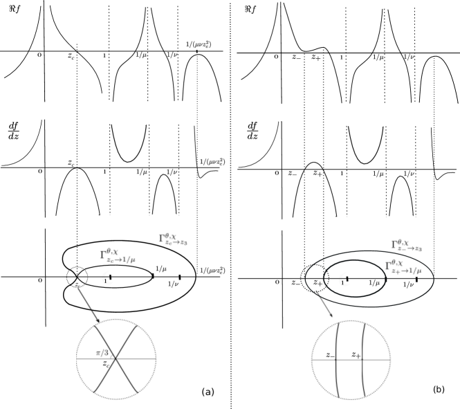
Figure 7: Schematic illustration of the behavior of $\Re f(\theta,\chi,z)$, of the derivative $f^{(0,0,1)}(\theta,\chi,z)$ and of the the steepest descent contours (a) $\Gamma_{z_{c}\to z_{3}}^{\theta,\chi}$ and $\Gamma_{z_{c}\to 1\mu}^{\theta,\chi}$ in the case $\chi=\chi(\theta)$ and (b) $\Gamma_{z_{-}\to z_{3}}^{\theta,\chi}$ and $\Gamma_{z_{+}\to 1/\mu}^{\theta,\chi}$ in the case $\chi<\chi(\theta).$

Correspondingly from the sign of

$$\frac{dz_{\pm}}{d\chi}=\frac{1-\nu}{\left(1-\nu z_{\pm}\right)\left(1-z_{\pm}\right)f^{(0,0,2)}(\theta,\chi,z_{\pm})}$$ (88)

coinciding with the sign of $f^{(0,0,2)}(\theta,\chi,z_{\pm})$ we see that as $\chi$ decreases down from $\chi(\theta)$, $z_{-}$ and $z_{+}$ move along the real axis away from $z_{c}$ towards the singularities at $z=0$ and $z=1,$ respectively. The left saddle point $z_{-}$ asymptotically approaches the origin as $\chi\to-\infty.$ The right saddle point $z_{+}$ crosses $z=1$, when $\chi=-\theta$ and moves further to the right as $\chi$ continues decreasing. However at $\chi=-\theta$ the extremum of $\Re f(\theta,\chi,z)$ at $z=z_{+}$ changes from maximum to minimum because the singularity of $f(\theta,\chi,z)$ changes the sign. That is an indication of the fact that when $\chi<-\theta$ the point $z=1$ becomes zero of the term $e^{-tf(\theta,\chi,z)}$ rather than a pole, and the corresponding integral vanishes.

When $\chi<\chi(\theta)$, the contours $\Gamma_{0}$ and $\Gamma_{1}$ in the double integral part of the kernel can be deformed into the steepest descent and ascent contours $\Gamma_{z_{-}}^{\theta,\chi}$ and $\Gamma_{z_{+}}^{\theta,\chi}$ respectively , which are the stationary phase contours being simple closed curves defined by equation

$$\Gamma_{z_{\pm}}^{\theta,\chi}=\left\{z:\Im f(\theta,\chi,z)=0\right\}.$$

with $z_{-}$ or $z_{+}$ being the points in $(0,1)$ where the contours cross the real axis. The steepest descent and ascent contours starting from the saddle points must be closed either via another saddle point or via a singularity, since $\Re f(\theta,\chi,z)$ is monotonous everywhere on stationary phase contours except at these points. Only one such a possibility exists in the range of interest of $\chi$. Specifically, for general $\chi<\chi(\theta)$ the contour $\Gamma_{0}$ is deformed to the steepest descent contour $\Gamma_{z_{-}\to z_{3}}^{\mathrm{\theta,\chi}}$ starting at $z_{-}$ and being closed via the third saddle point $z_{3}\in(1/\nu,\infty)\cup(-\infty,0)$ located on the positive or negative parts of the real axis when $\nu>0$ and $\nu<0$, respectively. In the latter case, the contour $\Gamma_{0}$ should be deformed via infinity, where the integrand is regular.

The steepest ascent version of $\Gamma_{1}$ is the contour $\Gamma_{z_{+}\to 1/\mu}^{\theta,\chi}$ outgoing from $z_{+}$, looping around $z=1$ and terminating at $z=1/\mu.$ For generic values of $\theta$ and $-\theta<\chi<\chi(\theta)$ the steepest descent and ascent contours cross the real axis at $z_{-}$ and $z_{+}$ respectively at the angle $\pi/2$, while when $\chi=\chi(\theta)$ the contours approach the double saddle point $z_{c}$ at angles divisible by $\pm\pi/3$ and $\pm 2\pi/3$.

As was noted above, when $\chi<-\theta$, the integral along $\Gamma_{1}$ vanishes, since zero of the integrand is at $z=1$ in this case. Also, it is easy to argue that the contours $\Gamma_{z_{-}\to z_{3}}^{\mathrm{\theta,\chi}}$ and $\Gamma_{z_{+}\to 1/\mu}^{\theta,\chi}$ corresponding to different values of $\chi<\chi(\theta)$ are always nested in the same way as for $\chi=\chi(\theta)$. Indeed, the contours separate the domains with opposite signs of $\Im$$f(\theta,\chi,z).$ Observing that $\mathrm{sgn}(\Im\log\left[(1-u)/(1-\nu u)\right]=\mathrm{-sgn}(\Im u)$, we see that as $\chi$ decreases, the contours should move outward with respect to the domain between them to compensate the change of $\Im f(\theta,\chi,z)$.

When $\chi>\chi(\theta)$ the two roots $z_{\pm}$ turn into a pair of complex conjugate roots, and the picture of the steepest descent contours becomes substantially different. Thus, the arguments below based on the picture described fail in that case. Fortunately, by conditions of the lemma the positive values of $(\chi-\chi(\theta))$ we are interested in are as small as $O(t^{-1/3})$. For this case of the variable $s$ taking values in bounded sets we will need only the first part of the analysis, which is insensitive to the sign of $(\chi-\chi(\theta))$, being an extension of $\chi=\chi(\theta)$ case.

(Bounded sets) Suppose first $s\in[\underline{s},\bar{s}]$ and $q\in[0,\underline{q}]$ for some $\bar{s}>\underline{s}$ and $\underline{q}\geq 0$. We outline the proof for $\Phi_{t\theta_{r}-j}^{t\theta_{r}}.$ The proof for $\tilde{\Psi}_{t\theta_{r}-j}^{t\theta_{r}}$ is completely analogous. The integration contour we use is the steepest descent contour $\Gamma_{z_{c}\to z_{3}}^{\mathrm{\theta,\chi(\theta)}}$ of the function $f(\chi(\theta),\theta,z)$, when the two saddle points have merged into the double saddle point, $z_{-}=z_{+}=z_{c}.$ Then, for some small $\epsilon>0$ we drop the part of the integral over $\Gamma_{z_{c}\to z_{3}}^{\mathrm{\theta,\chi(\theta)}}$ beyond the $\epsilon-$neighborhood $U_{\epsilon}(z_{c})=\{z:|z-z_{c}|<\epsilon\}$ of the double saddle point. For the contour being steepest descent this yields the error of order of $O\left(\exp(t\left(f(\chi(\theta),\theta,z_{c})-\delta\right))\right).$

Limiting the integration to the part of the contour inside $U_{\epsilon}(z_{c})$ we use the approximation for the integrand, which yields

$$\frac{1}{2\pi\mathrm{i}}\int_{\Gamma_{z_{c}\to z_{3}}^{\mathrm{\theta,\chi(\theta)}}\bigcap U_{\epsilon}(z_{c})}\frac{\exp\left(tf_{app}+aqt^{1/3}\left(\ln z_{c}+u/z_{c}\right)\right)}{z_{c}}du$$

where we use the notation $f_{app}$ for the Taylor approximation of $f(\chi_{r,s},\theta_{r},z_{c}+u)$ from the r.h.s. of (77). After making the variable change (78) this integral becomes

$$t^{-1/3}a^{-1}e^{tf(\chi_{r,s},\theta_{r},z_{c}(\theta_{r}))+aqt^{1/3}\ln z_{c}}e^{rq}\int_{t^{1/3}\epsilon e^{\mathrm{i}\left(\frac{2\pi}{3}+\epsilon_{1}\right)}}^{t^{1/3}\epsilon e^{-\mathrm{i}\left(\frac{2\pi}{3}+\epsilon_{1}\right)}}e^{-\frac{(u-r)^{3}}{3}+(s+q)(u-r)}du.$$

Here we replaced the the upper and lower half of the contour by two segments of rays approaching the origin at the angles $\pm\left(\frac{\pi}{3}+\epsilon_{1}\right),$ where $\epsilon_{1}$ is an $\epsilon-$dependent constant, which can be made small by choosing the $\epsilon$ small enough. Finally, shifting the integration contour by $r$ horizontally for the price of the error of order of $O(e^{-t\epsilon^{3}})$ coming from the boundary of $U_{\epsilon}$ and sending $t$ to infinity we arrive at the integral representation of the Airy function (34)

To estimate the error coming from the approximation we first note that the Taylor expansion (77) is obtained with error

$$f(\chi_{r,s},\theta_{r},z_{c}+u)-f_{app}(\chi_{r,s},\theta_{r},z_{c}+u)\,\,\,\,\,\,\,\,\,\,\,\,\,\,\,\,\,\,\,\,\,\,\,\,\,\,\,\,\,\,\,\,\,\,\,\,\,\,\,\,\,\,\,\,\,\,\,\,\,\,\,\,\,\,\,\,\,\,$$ (89)

$$=c_{0}t^{-4/3}+c_{1}t^{-1}u+c_{2}t^{-2/3}u^{2}+c_{3}t^{-1/3}u^{3}+c_{4}u^{4},$$

where $c_{0},\dots,c_{4}$ are some constants. Then, the corrections to the integrand satisfy

$$\left|e^{tf+(aqt^{1/3}-1)\ln(z_{c}+u)}-e^{tf_{app}+(aqt^{1/3}-1)(\ln z_{c}+u/z_{c})}\right|$$

$$\leq \left|e^{tf_{app}+(aqt^{1/3}-1)\ln z_{c}}\right|\left|e^{c_{0}t^{-1/3}+c_{1}|u|+c_{2}t^{1/3}|u|^{2}+c_{3}t^{2/3}|u|^{3}+tc_{4}|u|^{4}}-1\right|$$ (90)

$$\leq \left|e^{tf_{app}+(aqt^{1/3}-1)\ln z_{c}}\right|e^{c_{0}t^{-1/3}+\epsilon\left(c_{1}+c_{2}t^{1/3}|u|+c_{3}t^{2/3}|u|^{2}+tc_{4}|u|^{3}\right)}$$

$$\times \left|c_{0}t^{-1/3}+c_{1}|u|+c_{2}t^{1/3}|u|^{2}+c_{3}t^{2/3}|u|^{3}+tc_{4}|u|^{4}\right|,$$

where the first inequality uses the estimate (89) and the second uses the inequality $|e^{x}-1|\leq xe^{x}$ for $x>0$ and the fact that the integrand is limited to $|u|<\epsilon$. The modulus of the difference of $\Phi_{t\theta_{r}-j}^{t\theta_{r}}$ and its approximation is majorized by the integral of the first line of this expression over the contour $\Gamma_{z_{c}\to z_{3}}^{\mathrm{\theta,\chi(\theta)}}\bigcap U_{\epsilon}$. Making the variable change (78) and sending $t\to\infty$ we observe that the integral of the last two lines r.h.s. of (90) is convergent for $\epsilon$ small enough and is

$$O(t^{-2/3}e^{tf(\chi_{r,s},\theta_{r},z_{c}(\theta_{r}))+aqt^{1/3}\ln z_{c}})=O\left(\left|\Phi_{t\theta_{r}-aqt^{1/3}}^{t\theta_{r}}(t\chi_{r,s})\right|t^{-1/3}\right).$$

(Arbitrary sets) The next step is to extend this estimate to arbitrary values of $s$ and $j$. We first prove the statements for particular case $j=0$ and then extend to arbitrary $j>0$. To perform the analysis of the integrals in the case $\chi<\chi(\theta)$ we use the steepest descent and ascent integration contours $\Gamma_{z_{-}\to z_{3}}^{\mathrm{\theta,\chi}}$ and $\Gamma_{z_{+}\to 1/\mu}^{\theta,\chi}$ for $\Phi$ and $\tilde{\Psi}$. The corresponding integrals hence are bounded by the maxima of the integrands at these contours. To show that the points $z_{-},z_{+}\in(0,1)$ defined by $f^{(0,0,1)}(\chi,\theta,z_{\pm})=0$ are the minimum and maximum of $f(\chi,\theta,z)$ respectively we note that

$$f^{(0,0,2)}(\chi,\theta,z_{\pm})\lessgtr 0$$ (91)

when $\chi<\chi(\theta)$ for $z_{-}$ and for $-\theta<\chi<\chi(\theta)$ for $z_{+}.$ To this end we note that though the derivatives $dz_{\pm}/d\chi$ diverge as $\chi\to\chi(\theta)$, $z_{-}$ and $z_{+}$ are smooth functions of

$$\zeta=\sqrt{\chi(\theta)-\chi}.$$

In terms of $\zeta$ we have,

$$\left.\frac{df^{(0,0,2)}(\chi(\theta)-\zeta^{2},\theta,z_{\pm})}{d\zeta}\right|_{\zeta=0}=\left.\frac{dz_{\pm}}{d\zeta}\right|_{\zeta=0}f^{(0,0,3)}(\chi(\theta),\theta,z_{c}),$$ (92)

where

$$f^{(0,0,3)}(\chi(\theta),\theta,z_{c})=-\frac{2(1-\mu)(\mu-\nu)\left(1-\mu\nu z_{c}^{3}\right)}{(1-z_{c})z_{c}(1-\mu z_{c})^{3}(1-\nu z_{c})\left(1-\nu z_{c}^{2}\right)}<0$$

and

$$\left.\frac{dz_{\pm}}{d\zeta}\right|_{\zeta=0} =\pm\alpha,$$ (93)

$$\mathrm{with}\qquad\alpha=\sqrt{\frac{2f^{(1,0,1)}(\chi(\theta),\theta,z_{c})}{f^{(0,0,3)}(\chi(\theta),\theta,z_{c})}}=\sqrt{\frac{(1-\nu)z_{c}(1-\mu z_{c})^{3}\left(1-\nu z_{c}^{2}\right)}{(1-\mu)(\mu-\nu)\left(1-\mu\nu z_{c}^{3}\right)}}>0.$$

As $f^{(0,0,2)}(\chi(\theta),\theta,z_{c})$ is zero, while its derivative in $\zeta$ is not, the inequalities (91) hold for small values of $\zeta>0$. Furthermore, they can be extended to the whole domain of interest, because the opposite would imply that $f^{(0,0,2)}(\chi(\theta),\theta,z)$ vanishes at more then one point in $(0,1)$, i.e. $z_{c}$ that solves eqs.(75) for given $\chi$ and $\theta$ is not unique. However, both $\chi(z_{c})$ and $\theta(z_{c})$ defined by (18,19) are monotonous functions of $z_{c}\in(0,1)$, which can be seen by direct differentiation, and, hence, are one-to-one.

From here we conclude that $f(\chi,\theta,z)$ is increasing when $z_{-}<z<z_{+},$ and there exist $\delta$ such that

$$\left|f(\chi,\theta,z_{\pm})-f(\chi,\theta,z_{c})\right|>\delta.$$

Thus, we first state that given $\theta>0$, $\epsilon>0$ and $\chi<\chi(\theta)-\epsilon$ there exists $\delta$, such that

$$\tilde{\Psi}_{t\theta}^{t\theta}(t\chi) =O\left(e^{-tf(\chi,\theta,z_{c}(\theta))-t\delta}\right),$$ (94)

$$\Phi_{t\theta}^{t\theta}(t\chi) =O\left(e^{tf(\chi,\theta,z_{c}(\theta))-t\delta}\right).$$ (95)

Second, we note that we can limit the integration by small $\epsilon$-vicinities $U_{\epsilon}(z_{\pm})$ of the the critical points, introducing another error of order of $O(e^{-\delta_{1}t})$.

Third, within $U_{\epsilon_{1}}(z_{\pm})$ and for $\chi(\theta)-\chi<\epsilon_{2}$ with some small $\epsilon_{1},\epsilon_{2}>0$ we can approximate $f(\chi,\theta,z)$ by its Taylor expansion near the critical points, with coefficients given by expansions in $\zeta$ . Using (92) and (93) we obtain

$$z_{\pm}=z_{c}\pm\alpha\zeta+O(\zeta^{2}).$$ (96)

After substituting this into $f(\chi,\theta,z_{\pm})$ and its derivatives with respect to the last argument we have.

$$f(\chi,\theta,z_{\pm})= f(\chi(\theta),\theta,z_{c})+\zeta^{2}f^{(1,0,0)}(\chi,\theta,z_{c})$$ (97)

$$\mp\frac{2}{3}\alpha f^{(1,0,1)}(\chi,\theta,z_{c})\zeta^{3}+O\left(\zeta^{4}\right)$$

$$= f(\chi,\theta,z_{c})\pm\frac{2}{3}\frac{\zeta^{3}}{\kappa_{f}^{3/2}}+O\left(\zeta^{4}\right),$$

$$f^{(0,0,1)}(\chi,\theta,z_{\pm}) =0,$$ (98)

$$f^{(0,0,2)}(\chi,\theta,z_{\pm}) =\pm\alpha f^{(0,0,3)}(\chi,\theta,z_{c})\zeta+O(\zeta^{2})$$

$$=\mp 2\left(\frac{\left|f^{(0,0,3)}(\chi,\theta,z_{c})\right|}{2}\right)^{2/3}\frac{\zeta}{\sqrt{\kappa_{f}}}+O(\zeta^{2}),$$

$$f^{(0,0,3)}(\chi,\theta,z_{\pm}) =f^{(0,0,3)}(\chi,\theta,z_{c})+O\left(\zeta\right)$$ (99)

The first equation here is obtained by integrating relation $df(\chi,\theta,z_{\pm})/d\chi=f^{(1,0,0)}(\chi,\theta,z_{\pm})$, where all the dependence on $\chi$ in r.h.s. enters only through eq. (96).

Using the above estimates, let us substitute the Taylor expansion for $f(\chi,\theta,z)$ into the integral formula of $\Phi_{t\theta}^{t\theta}(t\chi)$ with $\zeta=\sqrt{s\kappa_{f}}t^{-1/3}<\sqrt{\epsilon_{2}}$, assuming that $s>0$ and $\epsilon_{2}$ is arbitrarily small.

$$\Phi_{t\theta}^{t\theta}(t\chi) \simeq O\left(e^{t\left(f(\chi,\theta,z_{c})-\delta\right)}\right)+e^{tf(\chi,\theta,z_{c})-\frac{2}{3}s^{3/2}+O(t^{-1/3}s^{2})}$$

$$\times \oint_{\Gamma_{z_{-}\to z_{3}}^{\mathrm{\theta,\chi}}\bigcap U_{\epsilon_{1}}(z_{-})}e^{t\left(z-z_{-}\right)^{3}\frac{f^{(0,0,3)}(\chi,\theta,z_{c})}{6}+\left(z-z_{-}\right)^{2}\left(\frac{f^{(0,0,3)}(\chi,\theta,z_{c})}{2}\right)^{2/3}t^{2/3}\sqrt{s}}$$

$$\times e^{O\left(t^{1/3}s(z-z_{-})^{2}\right)+O\left(t^{2/3}\sqrt{s}(z-z_{-})^{3}\right)+O\left(t\left(z-z_{-}\right)^{4}\right)}\frac{dz}{2\pi\mathrm{i}z}.$$

Then, we make the variable change

$$x=(z-z_{-})\left(tf^{(0,0,3)}(\chi,\theta,z_{c}))/2\right)^{1/3}+\sqrt{s}$$

$$\simeq(z-z_{c})\left(tf^{(0,0,3)}(\chi,\theta,z_{c}))/2\right)^{1/3}$$ (100)

in the integral and deform the contour for it to pass via the point $x=0$ ($z=z_{c}$ in the original variables). If we neglect the corrections, we find the integrand coinciding with the one appearing from integral representation of Airy function (34). We would like to make sure that the deformed integration contour also matches that definition. To this end, we note that the contour $\Gamma_{z_{-}\to z_{3}}^{\theta,\chi}$ leaves the domain $U_{\epsilon_{1}}(z_{-})$ through the points $z_{-}+\epsilon_{1}\exp({\pm\mathrm{i}(2\pi/3-\phi_{1})}),$ where the angle $\phi_{1}$ can be made small by choosing $\zeta$ small enough, in which case $\phi_{1}=\sqrt{3}\alpha\zeta/(2\epsilon_{1})+O\left(\zeta^{2}/\epsilon_{1}^{2}\right)$. The deformation changes the angles to $\pm(2\pi/3+\phi_{2})$ where $\phi_{2}=O(\zeta^{2}/\epsilon_{1}^{2})$, which can be made small by choosing $\epsilon_{1}$ and $\epsilon_{2}$ such that the ratio $\epsilon_{2}/\epsilon_{1}^{2}$ is small. This ensures that the integration contour in $x$-variable consists of two segments of rays approaching the real axis at angles close to $\pm\pi/3$, which matches with (34). The segments become the infinite rays in the limit $t\to\infty$.

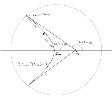
Figure 8: The steepest descend contour in $\epsilon_{1}$-vicinity of $z_{-}$ and its deformation passing through $z_{c}$.

Taking into account that with $st^{-2/3}=O(\epsilon_{2})$ the estimate

$$\left|e^{-\frac{2}{3}s^{3/2}+O(t^{-1/3}s^{2})}-e^{-\frac{2}{3}s^{3/2}}\right|=O(t^{-1/3}s^{2}e^{-\left(\frac{2}{3}-\sqrt{\epsilon_{2}}\right)s^{3/2}})=O(t^{-1/3}e^{-\delta_{1}s})$$

holds with any $\delta_{1}>0$, we obtain

$$\Phi_{t\theta}^{t\theta}(t\chi)=t^{-1/3}a^{-1}e^{tf(\chi,\theta,z_{c})}\left(\mathrm{Ai}(s)+O(e^{-\delta t})+O(t^{-1/3}e^{-\delta_{1}s})\right).$$ (101)

Similarly for $\tilde{\Psi}$ we have

$$\tilde{\Psi}_{t\theta}^{t\theta}(t\chi)=t^{-1/3}\kappa_{f}^{-1}e^{-tf(\chi,\theta,z_{c})}\left(\mathrm{Ai}(s)+O(e^{-\delta t})+O(t^{-1/3}e^{-\delta_{1}s})\right).$$ (102)

To extend these results to $\tilde{\Psi}_{t\theta-j}^{t\theta}(t\chi)$ and $\Phi_{t\theta-j}^{t\theta}(t\chi)$ with $j>0$ we note that from (84,85) and (74) that

$$\tilde{\Psi}_{t\theta-j}^{t\theta}(t\chi)=\tilde{\Psi}_{t(\theta-\xi)}^{t(\theta-\xi)}(t(\chi+\xi)),\,\,\,\Phi_{t\theta-j}^{t\theta}(t\chi) =\Phi_{t(\theta-\xi)}^{t(\theta-\xi)}(t(\chi+\xi)),$$

where we introduce notation $\xi=j/t$. Thus, the estimate of $\tilde{\Psi}_{t\theta-j}^{t\theta}(t\chi)$ and $\Phi_{t\theta-j}^{t\theta}(t\chi)$ is reduced to the previously studied case of $j=0$ with $\theta$ and $\chi$ replaced by $(\theta-\xi)$ and $(\chi+\xi)$ respectively.

Suppose first that $\chi(\theta)>\chi$ and $\xi>\epsilon$. Due to (87), there exists $\epsilon_{1}>0$ such that

$$\chi(\theta-\xi)-(\chi+\xi)>\epsilon_{1},$$

and hence, from (95,94)

$$\Phi_{t\theta-j}^{t\theta}(t\chi) =O(e^{tf(\chi+\xi,\theta-\xi,z_{c}(\theta-\xi))-t\delta}),$$

$$\tilde{\Psi}_{t\theta-j}^{t\theta}(t\chi) =O(e^{-tf(\chi+\xi,\theta-\xi,z_{c}(\theta-\xi))-t\delta})$$

in this case. Otherwise, when $\xi<\epsilon$, we apply the formulas (101,102) with $\theta$ and $\chi$ replaced by $(\theta_{r}-\xi)$ and $(\chi_{r,s,}+\xi)$ respectively. Using the approximations

$$\chi_{r,s}+\xi =\chi(\theta_{r}-\xi)+(\chi(\theta)-\chi(\theta_{r}-\xi)-s\kappa_{f}t^{-2/3})$$

$$=\chi(\theta_{r}-\xi)-t^{-2/3}\kappa_{f}\left(s+q\left(1+O(t^{-1/3})+O(\xi)\right)\right),$$

where we set set $\xi=t^{-2/3}q\frac{\kappa_{f}c(\theta)}{c(\theta)+1}=t^{-2/3}aq,$ and

$$f(\chi_{r,s}+\xi,\theta_{r}-\xi,z_{c}(\theta_{r}-\xi)) =f(\chi_{r,s},\theta_{r},z_{c}(\theta_{r}-\xi))+\xi\ln\left(z_{c}(\theta_{r}-\xi)\right)$$

$$=f(\chi_{r,s},\theta_{r},z_{c}(\theta_{r}))+ t^{-2/3}q\left(a\ln(z_{c}(\theta))+t^{-1/3}r+O(t^{-2/3})+O(\xi)\right)$$

we arrive at the statement of the lemma . ∎

With this estimates in hand we can estimate the double integral part of the kernel.

Corollary 2

Under conditions of lemma 4 there exists $\delta>0,$ such that for $t\to\infty$ the identity

$$t^{1/3}\kappa_{f}e^{t\left(f(\chi_{1},\theta_{1},z_{c}(\theta_{1}))-f(\chi_{2},\theta_{2},z_{c}(\theta_{2}))\right)}\widetilde{K}^{step}(n_{1},x_{1};n_{2},x_{2})$$

$$=\int_{0}^{\infty}e^{-q(r_{2}-r_{1})}\mathrm{Ai}(s_{1}+q)\mathrm{Ai}(s_{2}+q)dq+O\left(e^{-\delta t}\right) +O\left(e^{-\delta_{1}\left(s_{1}+s_{2}\right)}t^{-1/3}\right)$$

holds for any $\delta_{1}>0.$

Proof

The proof is based on the uniformity of the above estimates, where one should choose $\delta_{1}>(r_{1}-r_{2})/2$, and the fact that there is at most $O(t)$ summands in the sum (83). Finally, the sum converges to an integral as $t\to\infty$. ∎

Lemma 5

(Uniform estimate of the diffusive part of the kernel)

Given $r_{2}>r_{1}$, let $\theta_{i}=\theta_{r_{i}}$ and $\chi_{i}=\chi_{r_{i},s_{i}}$ for $i=1,2$ and $\theta_{r}$ and $\chi_{r,s}$ be as in (76). Then, the estimate

$$e^{t(f(\chi_{1},\theta_{1},z(\theta_{1}))-f(\chi_{2},\theta_{2},z(\theta_{2})))}\phi^{*(n_{1},n_{2},)}(x_{1},x_{2})$$

$$=\frac{t^{-1/3}}{2\kappa_{f}\sqrt{\pi(r_{2}-r_{1})}}e^{-\frac{\left(s_{2}+s_{1}\right)\left(r_{2}-r_{1}\right)}{2}+\frac{2}{3}\left(\frac{r_{2}-r_{1}}{2}\right)^{3}-\frac{\left(s_{1}-s_{2}\right)^{2}}{4(r_{2}-r_{1})}}$$

$$\times\left(1+O\left(t^{-1/3}e^{\epsilon\left(s_{1}-s_{2}\right)^{2}}\right)\right) +O\left(e^{-\epsilon t^{1/3}\frac{1}{2}(r_{2}-r_{1})}\right).$$

holds for any $s_{1},s_{2}$ and any small $\epsilon>0.$

Proof

The integral representation of the single integral part including the conjugation is given by

$$e^{tf(\chi_{1},\theta_{1},z(\theta_{1}))-f(\chi_{2},\theta_{2},z(\theta_{2}))}\phi^{*(n_{1},n_{2},)}(x_{1},x_{2})=\mathbbold{1}_{n_{2}>n_{1}}\oint_{\Gamma_{1}}\frac{dv}{2\pi\mathrm{i}}\frac{(\nu-1)e^{t^{2/3}h(v)}}{(1-\nu v)(1-v)},$$ (103)

where

$$h(v)=t^{1/3}\left(f(\chi_{1},\theta_{1},z_{c}(\theta_{1}))-f(\chi_{2},\theta_{2},z_{c}(\theta_{2}))-f(\chi_{1},\theta_{1},v)+f(\chi_{2},\theta_{2},v)\right).$$ (104)

We separated $t^{1/3}$ to ensure that $h(v)$ in its effective range survives in the limit $t\to\infty$ likewise the other equations below. In addition to the dependence of $h(v)$ on its argument, there is also dependence on $\chi_{1},\chi_{2}$ and $\theta_{1},\theta_{2}$, which we omit in the notation for brevity In fact the $v-$dependent part of the integrand depends only on relative coordinates

$$\delta\theta_{21}=\theta_{2}-\theta_{1},\,\,\,\delta\chi_{21}=\chi_{2}-\chi_{1}.$$

By definition the whole expression is nonzero when

$$\delta\theta_{21}>0.$$ (105)

Also, the integral is nonzero, when the integrand has a pole at $v=1$, i.e.

$$\delta\theta_{21}+\delta\chi_{21}\leq 0.$$ (106)

The stationary points of the integrand are defined by the equation

$$h^{\prime}(v) =t^{1/3}\left(\frac{(\delta\chi_{21}+\delta\theta_{21})\left(\nu-1\right)}{(1-v)(1-\nu v)}-\frac{\delta\theta_{12}}{v}\right)=0.$$ (107)

This yields a quadratic equation for $v$ that always has two real roots within the range of $\delta\theta_{21}$ and $\delta\chi_{21}$ specified. One can see that one of the roots is always in $(0,1)$ and the other is either in $(1,\infty)$ or in $(-\infty,0).$

This can be seen by using a parametrization

$$\delta\theta_{21}+\delta\chi_{21}=-e^{2y}\delta\theta_{21},\quad\nu=1-\left(\frac{\sinh x}{\sinh y}\right)^{2}$$

in terms of two parameters $x>0$ and $y\in(-\infty,\infty)$ consistent with (105,106). Then, the roots of (107) are

$$u_{\pm}=\frac{e^{\pm x}\sinh y}{\sinh(y\mp x)},$$

whose behavior as functions of $y$ is shown in fig. 9. Looking at the second derivative

$$h^{\prime\prime}(u_{\pm})=\pm t^{1/3}\delta\theta_{21}2e^{\pm 2x-y}\frac{\coth x\sinh^{2}(x\pm y)}{\sinh y},$$

we can see that it is positive at $u_{+}$, when $y<0$, and at $u_{-}$, when $y>0$.

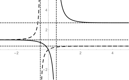
Figure 9: The stationary points $u_{+}$(solid line) and $u_{-}$(dashed line) as functions of $y$ with $x$ fixed. The roots $u_{\pm}$ diverge at $y=\pm x$ respectively (vertical dotted lines). The roots approach the limiting values $u_{\pm}\to 1$ as $y\to-\infty$ and $u_{\pm}\to e^{\pm 2x}$ as $y\to+\infty$ (horizontal dotted lines).

The stationary phase contour $\Gamma_{u_{+}\to u_{-}}$ defined by $\Im h(v)=0$ passes through both roots crossing the real axis traversally. In the two cases mentioned it is a simple loop around one of the poles of $h(u),$ either $u=1$ or $u=0$ respectively. In the former case it suits for $\Gamma_{1}$ as is and in the latter it can be obtained from $\Gamma_{1}$ by transforming via infinity, where $h(u)$ is regular.

It is clear from the above consideration that the critical point bringing the dominant contribution into the integral, i.e. the maximum of $h(v)$ at the steepest descent contour is always the root in $(0,1)$. We now denote this root $z^{*}$. It is a function of $\delta\chi_{21}$ for $\delta\theta_{21}$ fixed.

Once we have fixed the steepest descent contour, we expect that the order of the integral (103) is $O(e^{t^{2/3}h(z^{*})}).$

Remember that within the Fredholm determinant $\chi_{1}$ and $\chi_{2}$ are the rescaled running summation indices. Our first goal is to limit the range of their values by the domain, where the value of $h(z^{*})$ is close to the maximal one. An attempt to locate the maxima by looking for the values of $\chi_{1}$ and $\chi_{2}$ where the corresponding derivatives simultaneously vanish fails unless $\theta_{1}=\theta_{2}.$ Note, however, that the range of $\chi_{1}$ and $\chi_{2}$ within the sum representing the Fredholm determinant is bounded from above. Therefore, it is enough to argue that $h(z^{*})$ decays in the direction of summation. To this end, let us introduce auxiliary variables

$$\mathcal{X}=\frac{\chi_{1}+\chi_{2}+\theta_{1}+\theta_{2}}{2},\,\,\,\Delta=t^{1/3}\frac{\delta\chi_{21}+\delta\theta_{21}}{2}.$$ (108)

Observe that the $h(z)$ can be split into parts depending either on $\mathcal{X}$ or on $\Delta$ and $z$ or on neither of them.

$$h(z)=h_{1}(\Delta,z)+\mathcal{X}h_{2}+h_{3}$$

Here

$$h_{1}(\Delta,z) =\Delta\ln\left(\left(\frac{1-z}{1-\nu z}\right)^{2}\frac{1-\nu z_{c}(\theta_{1})}{1-z_{c}(\theta_{1})}\frac{1-\nu z_{c}(\theta_{2})}{1-z_{c}(\theta_{2})}\right)$$

$$\,\,\,\,\,\,\,\,\,\,\,\,\,\,\,\,\,\,\,\,\,\,\,\,\,\,\,\,\,\,\,\,\,\,\,\,\,\,\,\,-t^{1/3}\delta\theta_{21}\ln\left(\frac{z}{\sqrt{z_{c}(\theta_{1})z_{c}(\theta_{2})}}\right)$$

and

$$h_{2} =t^{1/3}\ln\left(\frac{1-z_{c}(\theta_{1})}{1-\nu z_{c}(\theta_{1})}\frac{1-\nu z_{c}(\theta_{2})}{1-z_{c}(\theta_{2})}\right)=$$

$$=\frac{2\text{$\kappa_{c}$}(r_{2}-r_{1})(1-\nu)z_{c}^{\prime}(\theta)}{(1-z_{c}(\theta))(1-\nu z_{c}(\theta))}+O(t^{-1/3})=\frac{(r_{2}-r_{1})}{\kappa_{f}}+O(t^{-1/3})>0$$

$$h_{3} =t^{1/3}\left(\frac{\theta_{1}+\theta_{2}}{2}\ln\frac{z_{c}(\theta_{2})}{z_{c}(\theta_{1})}+\ln\left(\frac{1-\nu z_{c}(\theta_{1})}{1-\mu z_{c}(\theta_{1})}\frac{1-\mu z_{c}(\theta_{2})}{1-\nu z_{c}(\theta_{2})}\right)\right)$$

$$=\frac{2\left(r_{1}-r_{2}\right)\kappa_{c}}{\theta^{\prime}(z_{c})}\left(\frac{\mu}{1-\mu z_{c}(\theta)}-\frac{\nu}{1-\nu z_{c}(\theta)}+\frac{\theta}{z_{c}(\theta)}\right)+O(t^{-1/3})$$

When $z=z^{*}$, the function $h_{1}(\Delta,z^{*})$ achieves a maximum at a single point $\Delta_{c}$. Note that in addition to the explicit $\Delta-$dependence in $h_{1}(\Delta,z)$, it depends on $\Delta$ through $z^{*}$. Recalling that $z=z^{*}$ is a critical point of $h_{1}(\Delta,z)$, we obtain the equation for $\Delta_{c}$ in the form

$$\left.\frac{dh_{1}(\Delta,z^{*})}{d\Delta}\right|_{\Delta=\Delta_{c}}=h_{1}^{(1,0)}(\Delta_{c},z^{*})=0.$$

This yields an equation

$$g(z^{*}(\Delta_{c}))=\frac{1}{2}\left(g(z_{c}(\theta_{1}))+g(z_{c}(\theta_{2}))\right),$$

where $z_{c}^{*}$ is $z^{*}$ evaluated at $\Delta=\Delta_{c}$ and

$$g(z)=f^{(1,0,0)}(\chi,\theta,z)=\ln\frac{1-z}{1-\nu z}.$$

Solving the equation perturbatively in powers of $t^{-1/3}$ up to the third order terms we obtain

$$z_{c}^{*} =z_{c}(\theta)+\kappa_{c}(r_{1}+r_{2})z_{c}^{\prime}(\theta)t^{-1/3}$$

$$+\frac{1}{2}\kappa_{c}^{2}\left(\frac{(r_{2}-r_{1})^{2}\left(z_{c}^{\prime}(\theta\right)^{2}g^{\prime\prime}(z_{c}(\theta))}{g^{\prime}(z_{c}(\theta))}+2\left(r_{1}^{2}+r_{2}^{2}\right)z_{c}^{\prime\prime}(\theta)\right)t^{-2/3}$$ (109)

$$+O(t^{-1})$$

To find $\Delta_{c}$ explicitly we substitute $z_{c}^{*}$ back to the stationary point equation (107), which can be recast in the following form.

$$\Delta_{c} =\frac{t^{1/3}\delta\theta_{21}}{2z^{*}g^{\prime}(z^{*})},$$

which together with (109) yields

$$\Delta_{c}=\kappa_{c}(r_{2}-r_{1})(1+\chi^{\prime}(\theta))+\kappa_{c}^{2}(r_{2}^{2}-r_{1}^{2})\chi^{\prime\prime}(\theta)t^{-1/3}+O\left(t^{-2/3}\right),$$ (110)

where we exploit the relation

$$\chi^{\prime}(\theta)=-\frac{1}{c(\theta)}=\frac{1}{z_{c}(\theta)g^{\prime}(z_{c}(\theta))}-1.$$

following from the formula (16) of the density $c$ and the relation (219).

It is also not difficult to check that at $h_{1}(\Delta,z^{*})$ is concave in $\Delta$. That the second derivative

$$\frac{d^{2}h_{1}(\Delta,z^{*})}{d\Delta^{2}} =-\frac{\left(h_{1}^{(1,1)}(\Delta,z^{*})\right)^{2}}{h_{1}^{(0,2)}(\Delta,z^{*})}$$ (111)

$$=-\frac{(1-\nu)^{2}}{\delta\theta_{21}t^{1/3}\left(1-1/z^{*}\right)^{2}\left(1-\nu z^{*}\right)^{2}-2\Delta(1-\nu)\left(1+\nu-2\nu z^{*}\right)},$$

is negative is easily seen from the $x-y$ parametrization

$$(\ref{eq: d2h/dDelta2})=\frac{\left|\coth y-1\right|\tanh x}{4\Delta}<0$$

and from the fact that $\Delta<0.$ Thus, $\Delta_{c}$ is indeed the maximum.

Now, we are in position to push forward the necessary estimates. First we recall that within the Fredholm sum (4) the rescaled summation indices decrease down from $\chi_{i}=\chi(\theta_{i})+O(t^{-1/3}),\,\,i=1,2$. Obviously the integral (103) of interest is close to maximal, when $\mathcal{X}=\mathcal{X}_{0}:=\left(\chi(\theta_{1})+\chi(\theta_{2})+\theta_{1}+\theta_{2}\right)/2$ and $\Delta=\Delta_{c}$, being $O(e^{t^{2/3}(h_{1}(\Delta_{c},z^{*}(\Delta_{c}))+\mathcal{X}_{0}h_{2}+h_{3})})$. Given $\epsilon>0$, when $\mathcal{X}_{0}-\mathcal{X>\epsilon}t^{-1/3}$, it is less at least by the factor $e^{-\frac{1}{2}(r_{2}-r_{1})(s_{2}+s_{1})}=O(e^{-\epsilon t^{1/3}\frac{1}{2}(r_{2}-r_{1})})$.

Let us consider the range of $\chi_{1},\chi_{2}$ where this inequality does not hold, i.e. when $\mathcal{X}_{0}-\mathcal{X<}\epsilon t^{-1/3},$ i.e.

$$-a_{i}t^{-2/3}<\chi(\theta_{i})-\chi_{i}<\epsilon t^{-1/3},\,\,\,i=1,2.$$

Obviously in this range

$$|\Delta-\Delta_{c}|<\epsilon$$ (112)

holds. Here, one can approximate $h(z)$ by the Taylor expansion. The three leading coefficients of the Taylor expansion are

$$h(z^{*}) = h(z_{c}^{*})+\frac{1}{2}\left.\frac{d^{2}h_{1}(\Delta,z^{*})}{d\Delta^{2}}\right|_{\Delta=\Delta_{c}}\left(\Delta-\Delta_{c}\right)^{2}+O\left(\left(\Delta-\Delta_{c}\right)^{3}\right)$$

$$= t^{-2/3}\left(\frac{2}{3}\left(\frac{r_{2}-r_{1}}{2}\right)^{3}-\frac{\left(s_{2}+s_{1}\right)\left(r_{2}-r_{1}\right)}{2}-\frac{\left(s_{1}-s_{2}\right)^{2}}{4(r_{2}-r_{1})}\right)$$

$$+O\left(\left(\Delta-\Delta_{c}\right)^{3}\right)$$

$$h^{\prime}(z^{*}) = 0$$ (114)

$$h^{\prime\prime}(z^{*}) = 2^{1/3}|f^{(0,0,3)}(\chi(\theta),\theta,z_{c}(\theta))|^{2/3}(r_{2}-r_{1})+O\left(\Delta-\Delta_{c}\right).$$ (115)

The most technical part here is the evaluation $h(z^{*}_{c})$ in the first line. To evaluate $h(z_{c}^{*})$ we use the expansion (77) of (104) and the formula (109) for $z_{c}^{*}.$ The second derivative of $h_{1}(\Delta,z^{*})$ in $\Delta$ is given in (111), where we should set $z^{*}=z_{c}^{*}$, and for $\Delta_{c}$ we use (110).

Let us denote the approximate value of $h(z^{*})$ given by (4.1) without the correction as $h_{app}(z^{*})$ . Then,

$$\left|e^{t^{2/3}h(z^{*})}-e^{t^{2/3}h_{app}(z^{*})}\right| = \left|e^{t^{2/3}h_{app}(z^{*})}\right|\left|1-e^{O\left(t^{2/3}(\Delta-\Delta_{c})^{3}\right)}\right|$$

$$\leq \left|e^{t^{2/3}h_{app}(z^{*})+O\left(t^{2/3}(\Delta-\Delta_{c})^{3}\right)}O\left(t^{2/3}(\Delta-\Delta_{c})^{3}\right)\right|,$$

from where we obtain

$$\left|e^{t^{2/3}h(z^{*})}-e^{-\frac{\left(s_{2}+s_{1}\right)\left(r_{2}-r_{1}\right)}{2}+\frac{2}{3}\left(\frac{r_{2}-r_{1}}{2}\right)^{3}-\frac{\left(s_{1}-s_{2}\right)^{2}}{4(r_{2}-r_{1})}}\right|\,\,\,\,\,\,\,\,\,\,\,\,\,\,\,\,\,\,\,\,\,\,\,\,$$

$$\leq O\left(e^{-\frac{\left(s_{2}+s_{1}\right)\left(r_{2}-r_{1}\right)}{2}+\frac{2}{3}\left(\frac{r_{2}-r_{1}}{2}\right)^{3}-\frac{\left(s_{1}-s_{2}\right)^{2}}{4(r_{2}-r_{1})}(1-\epsilon c_{1})}t^{-1/3}\left(s_{1}-s_{2}\right)^{3}\right)$$

with some $\epsilon-$independent constant $c_{1}>0$. Here we used the identity

$$\left(\Delta-\Delta_{c}\right)^{3}=t^{-1}\left(s_{1}-s_{2}\right)^{3}\kappa_{f}^{3}+O((s_{1}-s_{2})^{2}t^{-4/3})$$

following from (108,110) to estimate the pre-exponential factor and the inequality

$$\left|\Delta-\Delta_{c}\right|^{3}\leq\epsilon t^{-2/3}\left(s_{1}-s_{2}\right)^{2}\kappa_{f}^{2}$$

following from (112) to estimate the exponent. As $\epsilon$ can be chosen arbitrarily small, this is obviously an integrable function in the range $(s_{1},s_{2})\in[\underline{s},\infty)^{2}$.

For the integral part we have

$$(\nu-1)\int_{\Gamma_{1}} \frac{\exp\left(t^{2/3}\left(h(v)-h(z^{*})\right)\right)}{(1-\nu v)(1-v)}\frac{dv}{2\pi\mathrm{i}}$$

$$=(\nu-1)\int_{\Gamma_{u_{+}\to u_{-}}}\frac{e^{t^{2/3\left(2^{-2/3}|f^{(0,0,3)}(\chi(\theta),\theta,z_{c}(\theta))|^{2/3}(r_{2}-r_{1})\right)(v-z^{*})^{2}}}}{(1-\nu v)(1-v)}$$

$$\,\,\,\,\,\,\,\,\,\,\,\,\,\,\,\,\,\,\,\,\,\,\,\,\,\,\,\,\,\,\,\,\,\,\,\,\,\,\,\,\times e^{O\left(t^{1/3}\left(s_{1}-s_{2}\right)\right)(v-z^{*})^{2}+O\left(t^{2/3}\right)\left(v-z^{*}\right){}^{3}}\frac{dv}{2\pi\mathrm{i}}$$

$$=\frac{t^{-1/3}}{2\kappa_{f}\sqrt{\pi(r_{2}-r_{1})}}\left(1+O\left(e^{-\delta t^{2/3}}\right)+O\left(t^{-1/3}(s_{1}-s_{2})\right)\right).$$

Multiplying this integral by the estimate of $e^{t^{2/3}h(z^{*})}$ we come to the statement of the lemma. ∎

To prove the convergence of the Fredholm determinant we need the Kernel to be an integrable in variables $s_{1},s_{2}.$ The above uniform estimates are effective, when $s_{i}\ll t^{2/3}$ in the former case and when $s_{i}\ll t^{1/3}$ in the latter. Otherwise the limiting expression becomes comparable to the exponentially small correction, which have not been controlled yet. The large deviation estimates are necessary to fill this gap. In fact the large deviation estimate for the diffusive term was already obtained in course of proof of the lemma 5.

Corollary 3

For $\left(s_{1}+s_{2}\right)>\epsilon t^{1/3}$ and $t$ large enough

$$e^{tf(\chi_{1},\theta_{1},z(\theta_{1}))-f(\chi_{2},\theta_{2},z(\theta_{2}))}\phi^{*(n_{1},n_{2},)}(x_{1},x_{2})\leq e^{-(r_{2}-r_{1})\frac{s_{1}+s_{2}}{2}}.$$

The following lemma gives the one for the double integral part of the kernel.

Lemma 6

(Large deviation bound for the main part of the kernel.)

There exists small $\epsilon>0$, such that for $(s_{1},s_{2})\in[\underline{s},\infty)^{2}\backslash[\underline{s},\epsilon t^{2/3})^{2}$ and $t$ large enough

$$e^{t\left(f(\chi_{1},\theta_{1},z_{c}(\theta_{1}))-f(\chi_{2},\theta_{2},z_{c}(\theta_{2}))\right)}\widetilde{K}^{step}(n_{1},x_{1};n_{2},x_{2})\leq e^{-\delta(s_{1}+s_{2})},$$

for some $\delta>0$.

Proof

We first note that $\widetilde{K}^{step}(n_{1},x_{1};n_{2},x_{2})$ written as a sum is majorized by the maximal summand times the total number of summands, which is $O(t).$ Thus keeping the terms exponentially decaying with $t$ in the variable range under consideration and ignoring the power law factors we have

$$e^{t\left(f(\chi_{1},\theta_{1},z_{c}(\theta_{1}))-f(\chi_{2},\theta_{2},z_{c}(\theta_{2}))\right)}\left|\sum_{k=1}^{n_{2}}\tilde{\Psi}_{n_{1}-k}^{n_{1}}(x_{1})\Phi_{n_{2}-k}^{n_{2}}(x_{2})_{i}\right|$$ , (118)

$$\leq t\theta_{2}\exp\left(t\max_{\xi\in(0,\theta_{2})}\left(f_{2}^{-}(\xi)-f_{1}^{+}(\xi)\right)\right)$$

where

$$f_{i}^{\pm}(\xi)=f(\chi_{i}+\xi,\theta_{i}-\xi,z_{\pm}(\theta_{i}-\xi))-f(\chi_{i},\theta_{i},z_{c}(\theta_{i}))$$

for $i=1,2$. Suppose that

$$\chi(\theta)-\chi_{i}>\epsilon,\,\,\,i=1,2.$$ (119)

To maximize the difference in the exponent, we note that

$$\frac{d}{d\xi}\left(f_{2}^{-}(\xi)-f_{1}^{+}(\xi)\right)= \ln\frac{z_{-}(\chi_{2}+\xi,\theta_{2}-\xi)}{z_{+}(\chi_{1}+\xi,\theta_{1}-\xi)}$$ (120)

$$= \ln\frac{z_{-}(\chi_{2}+\xi,\theta-\xi)}{z_{+}(\chi_{1}+\xi,\theta-\xi)}+O\left(t^{-1/3}\right)<0.$$

Indeed, due to (87)

$$\chi(\theta-\xi)-(\chi_{i}+\xi)=(\chi(\theta-\xi)-\chi(\theta)-\xi)+(\chi(\theta)-\chi_{i})>\epsilon,$$

and for $z_{+}(\theta)$ $(z_{-}(\theta)$) being monotonously decreasing (increasing) function the inequality (120) holds. This suggests that the maximum is achieved at $\xi=0.$ At $\xi=0$ the the maximized expression is monotonously increasing in $\chi$ as it is a difference of increasing and decreasing parts, whose derivatives are

$$\frac{d}{d\chi_{i}}\left(f_{i}^{\pm}(0)\right)=\ln\left(\frac{\left(1-z_{\pm}\right)\left(1-\nu z_{c}(\theta)\right)}{\left(1-\nu z_{\pm}\right)\left(1-z_{c}(\theta)\right)}\right)\lessgtr 0.$$ (121)

Furthermore, as follows from

$$\frac{d^{2}}{d\chi_{i}^{2}}\left(f_{i}^{\pm}(0)\right)=\frac{dz_{\pm}}{d\chi}\frac{\nu-1}{\left(1-z_{\pm}\right)\left(1-\nu z_{\pm}\right)}\gtrless 0$$

$f_{i}^{+}(0)$ and $f_{i}^{-}(0)$ are convex and concave functions of $\chi_{i}$ respectively. Thus, the estimate for arbitrary $\chi_{i}<\chi(\theta)-\epsilon$ can be bounded by that with $\chi_{i}=\chi(\theta)-\epsilon$, i.e.

$$f_{i}^{\pm}(0) \gtreqless\left.f_{i}^{\pm}(0)\right|_{\chi_{i}=\chi(\theta)-\epsilon}+\left.\frac{df_{i}^{\pm}(0)}{d\chi_{i}}\right|_{\chi_{i}=\chi(\theta)-\epsilon}(\chi_{i}-\chi(\theta)+\epsilon)$$

$$=\pm\frac{2}{3}\frac{\epsilon^{3/2}}{\kappa_{f}^{3/2}}\mp\left(\frac{\sqrt{\epsilon}}{\kappa_{f}^{3/2}}+O(\epsilon)\right)(\epsilon-s_{i}\kappa_{f}t^{-2/3})+O(\epsilon^{2})$$

$$=\mp\frac{1}{3}\frac{\epsilon^{3/2}}{\kappa_{f}^{3/2}}\pm s_{i}\sqrt{\frac{\epsilon}{\kappa_{f}}}t^{-2/3}+O(\epsilon^{2})+O(\epsilon s_{i}t^{-2/3}),$$

where the first summand in the first line is approximated using (97) and the derivative in the second line is obtained from (121) and (96). Hence

$$f_{2}^{-}(0)-f_{1}^{+}(0) \leq\left(\frac{2}{3}\frac{\epsilon^{3/2}}{\kappa_{f}^{3/2}}-t^{-2/3}\sqrt{\frac{\epsilon}{\kappa_{f}}}\left(s_{2}+s_{1}\right)\right)\left(1+O(\sqrt{\epsilon})\right)$$

$$\leq-\frac{2t^{-2/3}}{3}\sqrt{\frac{\epsilon}{\kappa_{f}}}\left(s_{2}+s_{1}\right)\left(1+O(\sqrt{\epsilon})\right),$$

where we used inequalities (119), equivalent to $\kappa_{f}s_{i}t^{-2/3}>\epsilon$ for large $t$. It follows then, that for any $\delta>0$ and large enough $t$

$$\theta_{2}t\exp\left[t\left(f_{2}^{-}(0)-f_{1}^{+}(0)\right)\right]\leq e^{-\delta(s_{1}+s_{2})}.$$

If one of $\chi_{i}$ is inside the $\epsilon-$vicinity of $\chi(\theta)$, the same argument is used for the other variable, while for $f_{i}^{\pm}(0)$ we use (97), that yields

$$f_{i}^{\pm}(0)=\pm\frac{2}{3}s_{i}^{3/2}t{}^{-1}+O(\epsilon^{2}).$$

Then for example for $s<\chi_{1}-\chi(\theta)<\epsilon$ and we have

$$f_{2}^{-}(0)-f_{1}^{+}(0) \leq\left(\frac{1}{3}\frac{\epsilon^{3/2}}{\kappa_{f}^{3/2}}-\frac{2}{3}s_{1}^{3/2}t{}^{-1}-t^{-2/3}\sqrt{\frac{\epsilon}{\kappa_{f}}}s_{2}\right)\left(1+O(\sqrt{\epsilon})\right)$$

$$\leq-\left(\frac{2t^{-2/3}}{3}\sqrt{\frac{\epsilon}{\kappa_{f}}}s_{2}+\frac{2}{3}s_{1}^{3/2}t{}^{-1}\right)\left(1+O(\sqrt{\epsilon})\right),$$

which leads to the same estimate. ∎

Now we are in position to complete the proof of the first part of Theorem 2.2.

Proof

First we note that there exists $\delta>0,$ such that

$$K(n_{1},x_{1};n_{2},x_{2})\leq\mathrm{const}\,e^{-\delta\left(s_{1}+s_{2}\right)}.$$

Indeed, for the corrections and for the diffusive part this directly follows from the lemmas 4-6.The main part for is bounded by

$$\left|\int_{0}^{\infty}e^{-q(r_{2}-r_{1})}\mathrm{Ai}(s_{1}+q)\mathrm{Ai}(s_{2}+q)dq\right|$$

$$\leq \mathrm{\delta_{1}}\int_{0}^{\infty}e^{-q(r_{2}-r_{1})}e^{-\delta\left((s_{1}+q)+(s_{2}+q)\right)}dq$$

$$\leq \mathrm{const\,}e^{-\delta(s_{1}+s_{2})},$$

where the first inequality follows from the asymptotics of Airy function $\mathrm{Ai}(x)=O\left(e^{-\frac{2}{3}x^{3/2}}\right)$ for $x\to\infty$ and its boundedness, which in particular suggests that for any $\delta_{1}>0$ there exists $\delta$, such that $\mathrm{Ai}(x)<\delta e^{-\delta_{1}x}$ for $x>0$, while the integral converges if $\delta>r_{1}-r_{2}.$ Thus, by Hadamard inequality

$$\det_{1\leq i,j\leq n}K^{step}(n_{1},x_{1};n_{2},x_{2})\leq n^{n/2}\delta^{n}\prod_{i=1}^{n}e^{-\delta_{1}s_{i}},$$ (122)

and hence

$$\sum_{x_{1}\leq a_{1}}\cdots\sum_{x_{n}\leq a_{n}}\det_{1\leq i,j\leq n}K^{step}(n_{1},x_{1};n_{2},x_{2})\leq n^{n/2}\mathrm{const}^{n}.$$ (123)

This ensures the absolute convergence of the Fredholm sum (4) Then the summation in $x_{1},\dots,x_{n}$ and where estimates from lemmas 4-6 inserted into the sum and taking the limit $t\to\infty$ yield the Fredholm determinant with the Airy₂ kernel in the form

$$K_{\mathcal{A}_{2}}(r_{1},s_{1};r_{2},s_{2}) =-\mathbb{I}_{r_{2}>r_{1}}\left(4\pi\right)^{-1/2}e^{-\frac{\left(s_{2}+s_{1}\right)\left(r_{2}-r_{1}\right)}{2}+\frac{2}{3}\left(\frac{r_{2}-r_{1}}{2}\right)^{3}-\frac{\left(s_{1}-s_{2}\right)^{2}}{4(r_{2}-r_{1})}}$$

$$+\int_{0}^{\infty}e^{q(r_{1}-r_{2})}\mathrm{Ai}(s_{1}+q)\mathrm{Ai}(s_{2}+q)dq$$

plus the corrections vanishing in the limit $t\to\infty$. The latter formula can be reduced to the the definition (33) using the relation Johansson1

$$\int_{-\infty}^{\infty}e^{q(r_{1}-r_{2})}\mathrm{Ai}(s_{1}+q)\mathrm{Ai}(s_{2}+q)dq=\left(4\pi\right)^{-1/2}e^{-\frac{\left(s_{2}+s_{1}\right)\left(r_{2}-r_{1}\right)}{2}+\frac{2}{3}\left(\frac{r_{2}-r_{1}}{2}\right)^{3}-\frac{\left(s_{1}-s_{2}\right)^{2}}{4(r_{2}-r_{1})}}.$$

∎

4.2 Alternating initial configuration

The ideas used to prove the alternating IC case are very similar to that of the step IC. The asymptotic analysis of the kernels is performed with the steepest descent method. To prove the convergence of the Fredholm sum (4) we use the uniform convergence of the kernel on bounded sets of the summation variables and the large deviation bounds. The difference is in technical details, which we sketch below.

Saddle points and contour of steepest descent

We start the asymptotic analysis from the expression for the kernel (10) written in the form

$$K_{t}^{alt}(n_{1},x_{1};n_{2},x_{2})=(1-\nu)\frac{\mathbbold{1}_{r_{2}>r_{1}}}{2\pi i}\oint_{\Gamma_{1}}\frac{e^{t(f(\chi_{2},\theta_{2},v)-f(\chi_{1},\theta_{1},v))}}{(1-\nu v)(1-v)}dv$$ (124)

$$+\frac{1}{2\pi i}\oint_{\Gamma_{0}}\frac{dv}{v}e^{tf(\chi_{2},\theta_{2},v)-tf\left(\chi_{1},\theta_{1},\frac{1-v}{1-\nu v}\right)},$$

where $\chi_{i},\theta_{i}$ for $i=1,2$ have the same meaning as in (73) and the function $f(\chi,\theta,v)$ was defined in (74). As before, we will refer to the first integral as the diffusive part and to the second integral as the main part of the kernel.

The diffusive part integral is the same as in the case of step IC. Thus, we concentrate on the main part of the kernel. Let us make the variable change

$$\omega = 2\theta_{1}+2\theta_{2}+\chi_{1}+\chi_{2}-2v(1/2),$$ (125)

$$\psi = \chi_{1}-\chi_{2},$$ (126)

where

$$v(1/2)=2j_{\infty}(1/2)=\frac{\mu-\nu}{(1-\mu+\sqrt{1-\nu})\sqrt{1-\nu}}$$

is the particle velocity at $c=1/2$, obtained by substituting the solution $z_{c}\in[0,1]$ of eq. (16),

$$z_{c}=\frac{1}{1+\sqrt{1-\nu}},$$ (127)

into the formula (17).

Then, the exponent of the integrand has the following form

$$g(\omega,\psi,u) = \left(v(1/2)+\frac{\omega-\psi}{2}\right)\ln\frac{1-u}{1-\nu u}$$

$$- \left(v(1/2)+\frac{\omega+\psi}{2}\right)\ln u+\ln\left(\frac{(1-\nu u)(1-p+pu)}{(1-\mu u)}\right).$$

Referring to the conjecture (13) for the distance traveled by particle we assume the following scaling for $\theta_{i}=\theta_{r_{i}}$ and $\chi_{i}=\chi_{r_{i},s_{i}}$,

$$\theta_{r} = \frac{v(1/2)}{2}+2^{5/3}r\kappa_{c}t^{-1/3},$$ (129)

$$\chi_{r,s} = -2^{8/3}r\kappa_{c}t^{-1/3}-2^{1/3}s\kappa_{f}t^{-2/3}.$$ (130)

The variables $r$ and $s$ characterize the displacements of order of $t^{2/3}$ and $t^{1/3}$ of the corresponding quantities from their macroscopic positions, and, as before, we will use notations $\theta_{r_{i}},\chi_{r_{i},s_{i}}$ instead of $\theta_{i},\chi_{i}$, when we want to emphasize the dependence of the latter on these variables. Here and further within this subsection we imply that $\kappa_{c}=\kappa_{c}(1/2)$ and $\kappa_{f}=\kappa_{f}(1/2)$ are constants obtained by substituting $z_{c}$ from (127) to (20,21). A useful relation to be used in further calculations is

$$\kappa_{c}=\frac{\sqrt{1-\nu}}{2}\kappa^{2}_{f}.$$ (131)

In terms of $\omega,\psi$ this scaling has the form

$$\omega =-2^{1/3}(s_{1}+s_{2})\kappa_{f}t^{-2/3},$$ (132)

$$\psi =2^{8/3}r_{21}\kappa_{c}t^{-1/3}-2^{1/3}(s_{1}-s_{2})\kappa_{f}t^{-2/3},$$ (133)

where $r_{21}=r_{2}-r_{1}$. Note that in (129,130) we have chosen the macroscopic reference value of particle numbers $\theta=v(1/2)/2$ such that the corresponding value of the coordinates is $\chi=0$. Then, within the Fredholm sum (4) we will have $\chi_{i}\leq 0$ in most of the summation range, may be with exception of small $O(t^{-2/3})$ vicinity of $\chi_{i}=0$. This suggests that $\omega\leq 0$ and $|\psi|\leq-\omega$, when $|\omega|$ and $|\psi|$ are larger than $O(t^{-2/3})$ and $O(t^{-1/3})$ respectively.

To estimate the main part of the kernel in the limit $t\to\infty$ we have to locate the saddle points of the integrand in the range of values of $\omega$ and $\psi$. To this end, let us consider the function $g(\omega,\psi,z)$. It has logarithmic singularities at the points $z=0,1,1/\nu,1/\mu$ and $z=\eta$, where $\eta=(p-1)/p$. It also has four critical points defined by equation

$$g^{(0,0,1)}(\omega,\psi,z)=0,\\$$ (134)

which can be recast in the form of a degree 4 polynomial equation with real coefficients that has either 4 real or a pair of real and a pair of complex conjugate or two pairs of complex conjugate roots. Of course, the roots depend on $\omega$ and $\psi$.

Two roots may coincide, when $z$ simultaneously satisfies another equation

$$g^{(0,0,2)}(\omega,\psi,z)=0,$$ (135)

in which case we have a double saddle point of the inetgrand. It should obviously be real. The consistency of equations (134,135) implies a constraint on values of $\psi$ and $\omega$ having the form of a system of two linear equations, which can be solved to obtain $\omega=\omega(z)$ and $\psi=\psi(z)$ as functions of position of the double saddle point $z$. In particular, it can be readily checked that the position of the double saddle point $z=z_{c}$, where $z_{c}$ is defined by (127), yields $\omega(z_{c})=\psi(z_{c})=0$. It is more difficult to verify that this is the only solution $z\in[0,1]$ satisfying $\omega(z)\leq 0$. To this end, we represent the rational function $\omega(z)$ as a single fraction. Its denominator factorizes into a product of positive factors and the numerator is divisible by $(z-z_{c})^{2}$. Finally, the quotient of the numerator divided by $(z-z_{c})^{2}$ is a fifth degree polynomial in the variable $\sqrt{1-\nu}$ with manifestly positive coefficients. For the explicit expressions being cumbersome, we omit them.

Given two roots coinciding at $z_{c}$, we can find the other two roots from equation

$$v^{2}-v\left(\frac{1+\sqrt{1-\nu}}{\mu}+1\right)+\frac{1+\sqrt{1-\nu}}{\mu\nu}=0.$$ (136)

This equation has either two complex conjugate or two real roots, when $\nu>0$ or $\nu<0$ respectively. In the latter case, one of the roots is located in $(1/\nu,\eta)$ and the other in $(1/\mu,+\infty)$.

Thus, when $\omega=0,\psi=0$ the function $g(0,0,z)$ has the double saddle point at $z_{c}$. As $\omega$ decreases or $\psi$ deviates from zero, the double saddle point splits into two critical points $z_{+}>z_{-}$ located on the real line. One can see from fig. 10 that the point $z_{-}$ ($z_{+}$) is a minimum (maximum) along the real axis of the function $g(\omega,\psi,z)$.

To characterize the location of the roots $z_{\pm}$ consider first the case $\omega=0$. The equation (134) always has a solution $z_{1}=z_{c}$ independent of $\psi$. Indeed, the simpler equation $g^{(0,0,1)}(0,\psi,z)-g^{(0,0,1)}(0,0,z)=0$ leads to a quadratic equation for $z$ with one of the roots being $z=z_{c}$, while we have already shown that the second term in the l.h.s. vanishes at $z=z_{c}$. Since the double saddle point in $[0,1]$ exists only when $\psi=0$, the second root $z_{2}$ of (134) should deviate from $z_{c}$ as $\psi$ goes away from zero. The derivative

$$\frac{\partial z_{2}}{\partial\psi}=-\frac{g^{(0,1,1)}(0,\psi,z_{2})}{g^{(0,0,2)}(0,\psi,z_{2})}=\frac{1-2z_{2}+\nu z_{2}^{2}}{2(1-z_{2})z_{2}(1-\nu z_{2})g^{(0,0,2)}(0,\psi,z_{2})}>0$$ (137)

is positive, since the numerator is positive (negative), when $z_{2}<z_{c}(z_{2}>z_{c})$, as well as $g^{(0,0,2)}(0,\psi,z_{2})>0(<0)$ for $z_{2}$ being minimum (maximum) in this case. Thus, when $\omega=0$, $z_{-}=\min\{z_{2},z_{c}\}$ and $z_{+}=\max\{z_{2},z_{c}\}$. Note that the ratio in the r.h.s becomes $0/0$ indeterminate as $z_{2}\to z_{c}$, which however can be resolved using the L’Hospital’s rule showing that the derivative is actually continuous at this point.

To probe the regime $\omega<0$ we show that the sign of the derivative

$$\frac{\partial z_{\pm}}{\partial\omega}=-\frac{g^{(1,0,1)}(0,\psi,z_{\pm})}{g^{(0,0,2)}(\omega,\psi,z_{\pm})}=\frac{1-2\nu z_{\pm}+\nu z_{\pm}^{2}}{2(1-z_{\pm})z_{\pm}(1-\nu z_{\pm})g^{(0,0,2)}(\omega,\psi,z_{\pm})}\lessgtr 0,$$ (138)

coincides with that of $g^{(0,0,2)}(0,\psi,z_{2})$. In other words as $\omega$ decreases from zero, both roots move away from $z_{c}$ towards $z_{-}=0$ and $z_{+}=1$ respectively. Note that when $\psi,\omega\to 0$ and hence $z_{\pm}\to z_{c}$ the denominator vanishes, while the numerator stays finite. This is a signature of a non-analytic dependence of the roots on $\omega$ at $\omega=\psi=0$.

We also note that $z_{-}$ and $z_{+}$ cross the points $z_{-}=0$ and $z_{+}=1$ respectively, when the expressions in parenthesis being the coefficient of the first and second logarithms in (4.2) change their sign. As follows from fig. 10, then the extrema at these points change from minima to maxima and vice versa. For $z_{-}$, this leads to disappearance of the pole inside the integration contour, which causes the integral vanishing. Also, the change of the extremum at $z_{+}$ is not relevant for our discussion, since we will use only the contour passing through $z_{-}$.

Figure 10: Schematic illustration of behavior of $\Re g(\omega,\psi,u)$, $dg(\omega,\psi,u)/du$ and the steepest descent and ascent contours (a) $\Gamma_{z_{c}\to\eta},\Gamma_{z_{c}\to 1/\mu}$ for $(\omega,\psi)=(0,0)$, when the two critical points are merged together, and (b) $\Gamma_{z_{-}\to\eta}^{\omega,\psi},\Gamma_{z_{+}\to 1/\mu}^{\omega,\psi}$ for $\omega<0$, when there are two real critical points and $z_{-}<z_{c}<z_{+}$. The behavior of the steepest descent contours in the vicinity to critical points is shown in circles.

Finally, looking at the structure of the lines in complex plain, where the imaginary part of $g(0,0,z)=0$ vanishes, we conclude that two stationary phase contours $\Gamma_{z_{c}\to\eta}$ and $\Gamma_{z_{c}\to 1/\mu}$ can be drawn through $z_{c}$ being the simple loops closed around $z=0$ and $z=1$ via the singularities at $z=\eta$ and $z=1/\mu$ respectively, see fig. 10. Being the steepest descent and ascent contours for $\Re g(0,0,z)$ they approach the double saddle point $z=z_{c}$ at angles $\pm 2\pi/3$ and $\pm\pi/3$ to the real axis. The general structure is preserved by continuity as $z_{-}$ and $z_{+}$ go away from $z_{c}$. Then, we have two steepest descent contours, which we refer to as $\Gamma_{z_{-}\to\eta}^{\omega,\psi}$ and $\Gamma_{z_{+}\to 1/\mu}^{\omega,\psi}$, that cross the real axis perpendicularly. The contours $\Gamma_{z_{c}\to\eta}$ and $\Gamma_{z_{-}\to\eta}^{\omega,\psi}$ are those we use below in the steepest descent analysis of the main part of the kernel.

Convergence

Lemma 7

Given $r_{1},r_{2}>0,$ $\underline{s}\in\mathbb{R}$, let $n_{i}=t\theta_{r_{i}}$ and $x_{i}=t\chi_{r_{i},s_{i}}$ for $i=1,2$ where $\theta_{r}$ and $\chi_{r,s}$ are defined by (129) and (130). Then, there exist $\delta>0$, such that estimates

$$\tilde{K}_{t}^{alt}(n_{1},x_{1};n_{2},x_{2})= \kappa_{f}(2t)^{-1/3}z_{c}^{x_{2}-x_{1}}e^{\frac{2}{3}r_{21}^{3}+r_{21}(s_{2}+s_{1})}$$

$$\times \Big{(}\mathrm{Ai}\left(r_{21}^{2}+s_{2}+s_{1}\right)+O(e^{-\delta t})+O(t^{-1/3}e^{-\delta_{1}(s_{1}+s_{2})})\Big{)}$$

hold uniformly for $s_{i}>\underline{s}$ with any $\delta_{1}>0$.

Remark 3

The factor

$$e^{tg(\omega,\psi,z_{c})}=z_{c}^{x_{2}-x_{1}}$$ (139)

coming with the kernel here and below is the conjugation that does not affect the value of the Fredholm determinant.

Proof

(Bounded sets) Suppose first $s_{1},s_{2}\in[\underline{s},\bar{s}]$ for some $\bar{s}>\underline{s}$ . The integration contour we use is the steepest descent contour $\Gamma_{z_{c}\to\eta}$ of the function $g(0,0,z)$. Then, for some small $\epsilon>0$ we can drop the part of the integral along $\Gamma_{z_{c}\to\eta}$ beyond the $\epsilon-$neighborhood $U_{\epsilon}(z_{c})=\{z:|z-z_{c}|<\epsilon\}$ of the saddle point. For the contour being the steepest descent this yields an error of order of $O\left(\exp(-\delta_{\epsilon}t)\right).$

Limiting the integration to the part of the contour inside $U_{\epsilon}(z_{c})$ we use the Taylor expansion

$$g(\omega,\psi,u)=-\psi\ln z_{c}+t^{-1}\left(-\frac{1}{3}y^{3}+y^{2}(r_{2}-r_{1})+y(s_{1}+s_{2})\right)$$

$$+O\left(y^{4}t^{-4/3},y^{3}t^{-4/3},y^{2}t^{-4/3}\right),$$ (140)

where we make a variable change $y=t^{1/3}\kappa_{f}2^{1/3}(u-z_{c})/z_{c}$.

Using the notation $g_{app}$ for the part of (140) without correction we have

$$\int_{\Gamma_{z_{c}\to\eta}\bigcap U_{\epsilon}(z_{c})} \frac{\exp\left(tg_{app}\right)}{z_{c}}\frac{du}{2\pi\mathrm{i}}$$

$$=\frac{z_{c}^{x_{2}-x_{1}}}{(2t)^{1/3}\kappa_{f}}\int_{t^{1/3}\epsilon e^{-\mathrm{i}\left(\frac{2\pi}{3}+\epsilon_{1}\right)}}^{t^{1/3}\epsilon e^{\mathrm{i}\left(\frac{2\pi}{3}+\epsilon_{1}\right)}}e^{\frac{1}{3}(y^{3}+y^{2}r_{21}+y(s_{1}+s_{2})}\frac{dy}{2\pi i},$$

where we replaced the upper and the lower halfs of the contour by two segments of rays approaching the origin at the angles $\pm\left(\frac{\pi}{3}+\epsilon_{1}\right),$ where $\epsilon_{1}$ is an $\epsilon-$ dependent constant, which can be made small by choosing the $\epsilon$ small enough. Making another variable change $y\to(y-r_{21})$, shifting the integration contour by $r_{21}$ in horizontal direction for the price of another exponentially small correction and using the integral representation of the Airy function (1) we arrive at the expression reproducing the statement of the lemma up to correction terms.

Keeping in mind the exponentially small in $t$ corrections acquired in course of the above derivation we should also account for the corrections coming form Taylor approximation (140). This argument literally reproduces that used in the case of step IC (see e.g. similar estimate in lemma 4, eqs. (89,90)) and results in corrections of the form $O(t^{-2/3}e^{tg(\omega,\psi,z_{c})})$.

(Arbitrary sets) The next step is to extend this estimate to large values of $s_{1},s_{2}$ . Suppose first that $(s_{1}+s_{2})>\epsilon t^{2/3}$ for some small $\epsilon>0$. To analyze the main part of the kernel we use the steepest descent integration contour $\Gamma_{z_{-}\to\eta}^{\omega,\psi}$. The integral hence is bounded by the maximum of the integrand at this contour, attained at the point $z_{-}=z_{-}(\omega,\psi)\in(0,z_{c})$, i.e.

$$e^{-tg(\omega,\psi,z_{c})}\tilde{K}_{t}^{alt}(n_{1},x_{1};n_{2},x_{2})=O\left(e^{t(g(\omega,\psi,z_{-})-g(\omega,\psi,z_{c}))}\right).$$ (142)

In the case under consideration $\omega<-\epsilon_{0}$ with $\epsilon_{0}\simeq\kappa_{f}2^{1/3}\epsilon$, and we assume that $|\psi|\leq-\omega$. We want to show the r.h.s. of (142) is exponentially small in $t$, i.e. that there exist $\delta>0$ such that inequality

$$g(\omega,\psi,z_{c})-g(\omega,\psi,z_{-}(\omega,\psi))>\delta$$ (143)

holds. The l.h.s. of the above inequality is difficult to analyze directly as it depends on two variables. We, however, can use the fact that it is monotonous in $\psi$ since the derivative

$$\frac{d}{d\psi}\left(g(\omega,\psi,z_{c})-g(\omega,\psi,z_{-}(\omega,\psi))\right)=\frac{1}{2}\ln\left(\frac{(1-z_{-})z_{-}}{(1-\nu z_{-})z_{c}^{2}}\right)<0$$

is negative, when $z_{-}<z_{c}$. Thus, we can bound the difference by that at $\psi=-\omega$.

$$g(\omega,\psi,z_{c})-g(\omega,\psi,z_{-}(\omega,\psi))>g(\omega,-\omega,z_{c})-g(\omega,-\omega,z_{-}(\omega,-\omega))$$ (144)

To bound the r.h.s. of this inequality we reproduce the arguments of lemma 4. We note that the two quantities $g(\omega,-\omega,z_{\pm}(\omega,-\omega))$ depend non-analytically on $\omega$ at $\omega=0$ since $z_{\pm}(\omega,-\omega)$ does. Rather, they are analytic in the variable $\tilde{\zeta}=\sqrt{-\omega}$. In particular,

$$\left.\frac{d}{d\tilde{\zeta}}\right|_{\tilde{\zeta}=0}g^{(0,0,2)}\left(-\tilde{\zeta}^{2},\tilde{\zeta}^{2},z_{\pm}(-\tilde{\zeta}^{2},\tilde{\zeta}^{2})\right)=\pm\tilde{\alpha}g^{(0,0,3)}(0,0,z_{c}),$$

where

$$\tilde{\alpha}=\left|\frac{dz_{-}(\tilde{\zeta}^{2},\tilde{\zeta}^{2})}{d\tilde{\zeta}}\right|_{\tilde{\zeta}=0}=\sqrt{\frac{g^{(1,0,1)}(0,0,z_{c})}{g^{(0,0,3)}(0,0,z_{c})}}$$

and we used

$$g^{(1,0,1)}(0,0,z_{c}) = -\frac{1}{z_{c}},\quad g^{(0,1,1)}(0,0,z_{c})=0,$$ (145)

$$g^{(0,0,3)}(0,0,z_{c}) = -4\left(\frac{\kappa_{f}}{z_{c}}\right)^{3}.$$ (146)

As the second derivative $g^{(0,0,2)}\left(-\tilde{\zeta}^{2},\tilde{\zeta}^{2},z_{\pm}(-\tilde{\zeta}^{2},\tilde{\zeta}^{2})\right)$ is zero at $\tilde{\zeta}=0$ and its derivative is not, the inequalities

$$g^{(0,0,2)}\left(-\tilde{\zeta}^{2},\tilde{\zeta}^{2},z_{\pm}(-\tilde{\zeta}^{2},\tilde{\zeta}^{2})\right)\lessgtr 0$$

must hold for small $\tilde{\zeta}>0$. They can also be extended to arbitrary $\tilde{\zeta}$ since no other double saddle points appear in $(0,1)$. Thus, we conclude that $z_{-}(-\tilde{\zeta}^{2},\tilde{\zeta}^{2})$ and $z_{+}(-\tilde{\zeta}^{2},\tilde{\zeta}^{2})$ are minimum and maximum the function $g\left(-\tilde{\zeta}^{2},\tilde{\zeta}^{2},z\right)$ of the variable $z$ respectively and this function is monotonously increasing in $z_{-}(-\tilde{\zeta}^{2},\tilde{\zeta}^{2})<z<z_{+}(-\tilde{\zeta}^{2},\tilde{\zeta}^{2})$. In particular, there exists $\delta>0$ such that $\left(g(-\tilde{\zeta}^{2},\tilde{\zeta}^{2},z_{c})-g(-\tilde{\zeta}^{2},\tilde{\zeta}^{2},z_{-}(-\tilde{\zeta}^{2},\tilde{\zeta}^{2})\right)>\delta$, which yields (143).

Now suppose that $s_{1}+s_{2}<\epsilon t^{2/3}$. The critical points $z_{\pm}=z_{c}+u$ are to be found from

$$g^{(0,0,1)}(\omega,\psi,z_{c}+u) = \omega g^{(1,0,1)}(0,0,z_{c})+\psi g^{(0,1,1)}(0,0,z_{c})$$

$$+ u\omega g^{(1,0,2)}(0,0,z_{c})+u\psi g^{(0,1,2)}(0,0,z_{c})$$

$$+ \frac{u^{2}}{2}g^{(0,0,3)}(0,0,z_{c})+O(u^{3},u^{2}\omega,u^{2}\psi)=0.$$

assuming that $u,\omega,\psi$ are small. The involved derivatives are given explicitly by (146) and

$$g^{(1,0,2)}(0,0,z_{c})= \frac{1}{z_{c}^{2}}-\frac{1}{z_{c}^{2}\sqrt{1-\nu}},\ g^{(0,1,2)}(0,0,z_{c})=\frac{1}{z_{c}^{2}\sqrt{1-\nu}}.$$

Solving (4.2) for $u$ we obtain

$$u_{\pm}=\frac{z_{c}(2t)^{-1/3}}{\kappa_{f}}\left(r_{21}\pm\sqrt{r_{21}^{2}+s_{1}+s_{2}}\right)+O\left(\frac{s_{1}+s_{2}}{t^{2/3}}\right),$$ (148)

where we use scaling form of $\omega,\psi$ (132, 133) and the fact that $s_{1}+s_{2}\geq|s_{1}-s_{2}|$ to estimate the corrections.

The idea of the further analysis is to use the Taylor approximation of $g(\omega,\psi,z)$ in the vicinity $U_{\epsilon_{1}}(z_{-})$ of $z_{-}$ with some small $\epsilon_{1}>0$. To this end, we limit the integration to the part of the steepest descent contour $\Gamma_{z_{-}\to\eta}$ within this domain, getting the error of order of $O(e^{-\delta_{1}t})$ with some $\delta_{1}>0$. Then, we approximate the function $g(\omega,\psi,z)$ by its Taylor expansion near the critical point $z_{-}$. The approximations of the function and its derivatives at $z_{-}$ are obtained by substituting (148) into the exact expressions.

$$g(\omega,\psi,z_{-})=g(\omega,\psi,z_{c})+\frac{1}{t}\left(-\frac{2}{3}(r^{2}_{21}+s_{1}+s_{2})^{3/2}+\frac{2}{3}r^{3}_{21}+r_{21}(s_{2}+s_{1})\right)$$

$$\hskip 303.53267pt+O\left(\frac{(s_{1}+s_{2})^{2}}{t^{4/3}}\right),$$

$$g^{(0,0,1)}(\omega,\psi,z_{-})=0,$$

$$g^{(0,0,2)}(\omega,\psi,z_{-})=2^{5/3}\frac{\kappa_{f}^{2}}{z_{c}^{2}}\sqrt{r_{21}^{2}+s_{1}+s_{2}}t^{-1/3}+O\left(\frac{s_{1}+s_{2}}{t^{2/3}}\right),$$

$$g^{(0,0,3)}(\omega,\psi,z_{-})=-4\left(\frac{\kappa_{f}}{z_{c}}\right)^{3}+O\left(\frac{\sqrt{s_{1}+s_{2}}}{t^{1/3}}\right).$$ (149)

As a result we obtain

$$\tilde{K}_{t}^{alt} (n_{1},x_{1};n_{2},x_{2})=e^{tg(\omega,\psi,z_{c})-2/3(r^{2}_{21}+s_{1}+s_{2})^{3/2}+\frac{5}{3}r^{3}_{21}+r_{21}(s_{2}+s_{1})+O\left(\frac{s_{1}+s_{2}}{t^{1/3}}\right)}$$

$$\times\oint_{\Gamma_{z_{-}\to\eta}\bigcap U_{\epsilon}(z_{-})}e^{-t\left(z-z_{-}\right)^{3}\frac{2}{3}\left(\frac{\kappa_{f}}{z_{c}}\right)^{3}+\left(z-z_{-}\right)^{2}\left(\frac{\kappa_{f}}{z_{c}}\right)^{2}2^{2/3}t^{2/3}\sqrt{r^{2}_{21}+s_{1}+s_{2}}}$$

$$\times e^{O\left((z-z_{c})^{2}t^{1/3}(s_{1}+s_{2})\right)+O\left(t(z-z_{-})^{3}t^{2/3}\sqrt{s_{1}+s_{2}}\right)+O\left(t\left(z-z_{-}\right)^{4}\right)}\frac{dz}{2\pi\mathrm{i}z}$$

$$+O\left(e^{t\left(g(\omega,\psi,z_{c})-\delta\right)}\right)+O(t^{-2/3}e^{-\delta_{1}(s_{1}+s_{2})})$$

Finally, making the variable change

$$y=(2t)^{1/3}\left(z-z_{-}\right)\kappa_{f}/z_{c}-\sqrt{r_{21}^{2}+s_{1}+s_{2}},$$

transforming the contour accordingly as we did in lemma 4 and estimating the corrections with the use of inequality $|1-e^{x}|\leq|x|e^{|x|}$ we arrive at the statement of the lemma. ∎

Lemma 8

(Uniform estimate of the diffusive part of the kernel)

Under conditions of lemma 7 the following estimate

$$\phi^{*(n_{1},n_{2},)}(x_{1},x_{2})=\mathbbold{1}_{r_{2}>r_{1}}\frac{z_{c}^{x_{2}-x_{1}}(2t)^{-1/3}}{\kappa_{f}\sqrt{4\pi(r_{2}-r_{1})}}e^{-\frac{\left(s_{1}-s_{2}\right)^{2}}{4(r_{2}-r_{1})}}\times\left(1+O(t^{-1/3})\right)$$

holds uniformly for $|s_{1}-s_{2}|<\epsilon t^{1/3}$ with some $\epsilon>0$.

Proof

The integral representation of the diffusive part of the kernel including the conjugation is given by

$$\phi^{*(n_{1},n_{2},)}(x_{1},x_{2})e^{-tg(\omega,\psi,z_{c})}=\mathbbold{1}_{n_{2}>n_{1}}\oint_{\Gamma_{1}}\frac{dv}{2\pi\mathrm{i}}\frac{(\nu-1)e^{t^{2/3}\tilde{h}(v)}}{(1-\nu v)(1-v)},$$ (150)

where

$$\tilde{h}(v)=t^{1/3}\left(f(\chi_{2},\theta_{2},v)-f(\chi_{1},\theta_{1},v)-g(\omega,\psi,z_{c})\right).$$ (151)

We can see that the integrand is similar to the one in lemma 5 up to change of the function $h(v)$ by $\tilde{h}(v)$, with all the difference in $v$-independent part

$$g(\omega,\psi,z_{c})=f(\chi_{2},\theta_{2},z_{c})-f(\chi_{1},\theta_{1},z_{c})$$

instead of

$$f(\chi_{2},\theta_{2},z_{c}(\theta_{2}))-f(\chi_{1},\theta_{1},z_{c}(\theta_{1})).$$

Thus the proof requires a simplified version of the analysis of that lemma. Specifically, the function

$$\tilde{h}(z)=\tilde{h}_{1}(\Delta,z)=2\Delta\ln\left(\left(\frac{1-z}{1-\nu z}\right)\frac{1}{z_{c}}\right)-t^{1/3}\delta\theta_{21}\ln\left(\frac{z}{z_{c}}\right)$$

is a simplified version of $h_{1}(\Delta,u)$, one of three parts of the function $h(v)$ depending on the parameter $\Delta$ defined in (108), while the other two are absent. The estimate of interest for $\Delta$ close to the critical value $\Delta_{c}=-2^{2/3}\kappa_{c}r_{21}$, at which the integral is maximal, consists in evaluating the integral in the saddle point approximation, which is dominated by a single $\Delta$-dependent saddle point $z^{*}$ equal to $z_{c}$, when $\Delta=\Delta_{c}$. The analysis of the integral from lemma 5 applied without any changes then yields

$$(\nu-1)\int_{\Gamma_{1}}\frac{\exp\left(t^{2/3}\left(\tilde{h}(z)-\tilde{h}(z^{*})\right)\right)}{(1-\nu z)(1-z)}\frac{dz}{2\pi\mathrm{i}}$$

$$=\frac{(2t)^{-1/3}}{2\kappa_{f}\sqrt{\pi(r_{2}-r_{1})}}\left(1+O\left(e^{-\delta t^{2/3}}\right)+O\left(t^{-1/3}(s_{1}-s_{2})\right)\right),$$

while for $h(z^{*})$ we obtain

$$e^{t^{2/3}\tilde{h}(z^{*})}=e^{\left(-\frac{\left(s_{1}-s_{2}\right)^{2}}{4(r_{2}-r_{1})}\right)+O\left(\left(\Delta-\Delta_{c}\right)^{3}\right)},$$

which is valid when $s_{i}<\epsilon t^{1/3},i=1,2.$

For larger deviations of $\Delta$ from $\Delta_{c}$ the integral can be bounded simply by the saddle point value of the integrand. This estimate is slightly different from that in lemma 5 since the second part of $h(v)$ proportional to $(s_{1}+s_{2})$ is absent in the case of the alternating IC. Instead we use the concavity of $\tilde{h}_{1}(\Delta,z^{*})$ in $\Delta$ to show that

$$\tilde{h}_{1}(\Delta,z^{*})<\tilde{h}_{1}(\Delta_{c},z^{*})+\left.\frac{d^{2}\tilde{h}_{1}(\Delta,z^{*})}{d\Delta^{2}}\right|_{\Delta_{c}-2^{-2/3}\epsilon\kappa_{f}}2^{-2/3}\epsilon\kappa_{f}(\Delta-\Delta_{c})$$

$$=\tilde{h}_{1}(\Delta_{c},z^{*})-\frac{(\epsilon+O(\epsilon^{2}))t^{1/3}(s_{2}-s_{1})}{4(r_{2}-r_{1})},$$

when $\Delta<\Delta_{c}-2^{-2/3}\epsilon\kappa_{f}$, i.e. $s_{2}-s_{1}>\epsilon t^{1/3}$. For further details we address the reader to proof lemma 5. The last bound also proofs the next lemma. ∎

Lemma 9

(Large deviation bound for the diffusive part of the kernel.)

There exists a small $\epsilon>0$, such that for $|s_{1}-s_{2}|>\epsilon t^{1/3}$ and $t$ large enough

$$\phi^{*(n_{1},n_{2},)}(x_{1},x_{2})\leq\mathbbold{1}_{s_{2}>s_{1}}t^{-1/3}e^{tg(\xi,\psi,z_{c})}e^{-\delta(s_{2}-s_{1})},$$

for some $\delta>0$.

Lemma 10

(Large deviation bound for the main part of the kernel.)

There exists small $\epsilon>0$, such that for $(s_{1},s_{2})\in[\underline{s},\infty)^{2}\backslash[\underline{s},\epsilon t^{2/3})^{2}$ and $t$ large enough the inequality

$$\widetilde{K}_{t}^{alt}(n_{1},x_{1};n_{2},x_{2})\leq t^{-1/3}e^{tg(\omega,\psi,z_{c})}e^{-\delta(s_{1}+s_{2})},$$

holds for some $\delta>0$.

Proof

The integral can be majorized by the maximum of the integrand times the total length of contour, which is $O(1).$ Therefore, we consider only the exponential in $t$ terms. Ignoring the power law factors we have.

$$\widetilde{K}^{alt}(n_{1},x_{1};n_{2},x_{2})\sim e^{-tg(\omega,\psi,z_{c})}\exp({tg(\omega,\psi,z_{-}(\omega,\psi))}).$$

In this section, it is more convenient to use different variables

$$\omega_{1}=\frac{\omega+\psi}{2},\quad\psi_{1}=\frac{\omega-\psi}{2}.$$

Suppose that $s_{i}t^{-2/3}>\epsilon,i=1,2$ for some $\epsilon>0$. Thus, we want to estimate the function

$$g_{1}\left(\omega_{1},\psi_{1}\right):=g\left(\omega,\psi,z_{-}(\omega,\psi)\right).$$

Note that

$$\frac{\partial}{\partial\omega_{1}}g_{1}(\omega_{1},\psi_{1}) =-\ln z_{-}>0,$$ (152)

$$\frac{\partial}{\partial\psi_{1}}g_{1}(\omega_{1},\psi_{1}) =\ln\left(\frac{1-z_{-}}{1-\nu z_{-}}\right)<0,$$ (153)

$$\frac{\partial^{2}}{\partial\omega_{1}^{2}}g_{1}(\omega_{1},\psi_{1}) =-\frac{1}{z^{2}_{-}g^{(0,0,2)}(\omega,\psi,z_{-})}<0,$$

$$\frac{\partial^{2}}{\partial\psi_{1}^{2}}g_{1}(\omega_{1},\psi_{1}) =-\frac{(1-\nu)^{2}}{(1-z_{-})^{2}(1-\nu z_{-})^{2}g^{(0,0,2)}(\omega,\psi,z_{-})}<0,$$

$$\frac{\partial^{2}}{\partial\psi_{1}\partial\omega_{1}}g_{1}(\omega_{1},\psi_{1}) =-\frac{(1-\nu)}{(1-z_{-})(1-\nu z_{-})z_{-}g^{(0,0,2)}(\omega,\psi,z_{-})}<0.$$

To evaluate those derivatives we use the fact that $g^{(0,0,1)}(\omega,\psi,z_{-})=0$ and $g^{(0,0,2)}(\omega,\psi,z_{-})>0$ for $0<z_{-}<z_{c}$ being minimum. Thus, $g_{1}(\omega_{1},\psi_{1})$ is a convex function of $\omega_{1},\psi_{1}$. With

$$\omega_{0}=2^{5/3}(r_{2}-r_{1})\kappa_{c}t^{-1/3}-2^{1/3}\epsilon\kappa_{f},$$

$$\psi_{0}=2^{5/3}(r_{1}-r_{2})\kappa_{c}t^{-1/3}-2^{1/3}\epsilon\kappa_{f}.$$

the following inequality follows from the convexity.

$$g_{1}(\omega_{1},\psi_{1})\leq\left.\frac{\partial g_{1}(\omega_{1},\psi_{0})}{\partial\omega_{1}}\right|_{\omega_{1}=\omega_{0}}(\omega_{1}-\omega_{0})+\left.\frac{\partial g_{1}(\omega_{0},\psi_{1})}{\partial\psi_{0}}\right|_{\psi_{1}=\psi_{0}}(\psi_{1}-\psi_{0})$$

$$+g_{1}(\omega_{0},\psi_{0})={(\omega_{0}-\psi_{0})}\ln z_{c}-\frac{2}{3}(2\epsilon)^{3/2}-\ln z_{-}2^{1/3}\kappa_{f}(\epsilon-s_{1}t^{-2/3})$$

$$+\ln\left(\frac{1-z_{-}}{1-\nu z_{-}}\right)2^{1/3}\kappa_{f}(\epsilon-s_{2}t^{-2/3})+O(\epsilon t^{-1/3},\epsilon^{2})$$

$$=\left(\sqrt{2\epsilon}+O(\epsilon)\right)\left(2\epsilon-(s_{1}+s_{2})t^{-2/3}\right)-\frac{2}{3}(2\epsilon)^{3/2}$$

$$+(\omega_{1}-\psi_{1})\ln z_{c}+O(\epsilon t^{-1/3},\epsilon^{2})$$

Here we use (152,153) for the derivatives in the first line. For $z_{-}$ and $g_{1}(\omega_{0},\psi_{0})$ we use the estimates (149,148). The term $(\omega_{1}-\psi_{1})\ln z_{c}$ multiplied by $t$ and exponentiated will produce the conjugation (139). Hence

$$g_{1}(\omega_{1},\psi_{1})-(\omega_{1}-\psi_{1})\ln z_{c} \leq-(s_{1}+s_{2})t^{-2/3}\sqrt{2\epsilon}\left(1+O(\sqrt{\epsilon})\right)$$

It follows then, that for any $\delta>0$ and large enough $t$

$$\exp\left[t\left(g(\omega_{1},\psi_{1})-(\omega_{1}-\psi_{1})\ln z_{c}\right)\right]\leq e^{-2\delta(s_{1}+s_{2})}<t^{-1/3}e^{-\delta(s_{1}+s_{2})}.$$

The final estimate depends only on $s_{1}+s_{2}$. Thus it remains correct even if $s_{i}<\epsilon t^{2/3}$ for one of $i=1,2$. In this case we should replace $2\epsilon\to\epsilon+s_{i}/t^{2/3}.$ ∎

Now we are in a position to complete the proof of the second part of Theorem 2.2.

Proof

Using the above lemmas we can show that there exists $\delta>0,$ such that

$$t^{1/3}e^{-tg(\omega,\psi,z_{c})}K_{t}^{alt}(n_{1},x_{1};n_{2},x_{2})\leq C(\,e^{-\delta\left(s_{1}+s_{2}\right)}+\mathbbold{1}_{r_{2}>r_{1}}e^{-\delta|s_{2}-s_{1}|})$$

for constant $C$ independent of $t$. Following to Borodin2006 let us consider a kernel with conjugation

$$K_{t}^{alt,conj}(n_{k},x_{k};n_{j},x_{j})=e^{-tg(\xi,\psi,z_{c})}\frac{(1+s^{2}_{k})^{k}}{(1+s^{2}_{j})^{j}}K_{t}^{alt}(n_{k},x_{k};n_{j},x_{j}).$$ (154)

Assume that $r_{k}>r_{j}$ for $k>j$. Then, we have the bounds

$$C \left(\,e^{-\delta\left(s_{k}+s_{j}\right)}+e^{-\delta|s_{j}-s_{k}|}\right)\frac{(1+s^{2}_{k})^{k}}{(1+s^{2}_{j})^{j}}\leq\frac{C_{1}}{1+s_{j}^{2}},\,\,j>k$$ (155)

$$C \left(\,e^{-\delta\left(s_{k}+s_{j}\right)}\right)\frac{(1+s^{2}_{j})^{j}}{(1+s^{2}_{k})^{k}}\leq C_{2}e^{-(s_{k}+s_{j})},\,\,j\leq k$$ (156)

for some $C_{1}>0,C_{2}>0$ independent of $t$. Thus

$$t^{1/3}K_{t}^{alt,conj}(n_{k},x_{k};n_{j},x_{j})\leq\begin{cases}C_{2}\,e^{-\delta\left(s_{k}+s_{j}\right)},\,\,j\leq k\\ \frac{C_{1}}{1+s^{2}_{j}},\,\,\,\,\,\,\,\,\,\,\,\,\,\,\,\,\,\,\,\,\,\,\,j>k.\end{cases}$$

By Hadamard inequality

$$\det_{1\leq i,j\leq n}K^{alt}_{t}(n_{k},x_{k};n_{j},x_{j})\leq C_{3}t^{-n/3}n^{n/2}\prod_{j=1}^{n}\max\left\{\frac{C_{3}}{1+s^{2}_{j}},\,C_{1}e^{-\delta s_{j}}\right\},$$ (157)

and hence

$$\sum_{x_{1}\leq a_{1}}\cdots\sum_{x_{n}\leq a_{n}}\det_{1\leq k,j\leq n}K^{step}_{t}(n_{k},x_{k};n_{j},x_{j})\sim$$ (158)

$$(C_{4}t^{1/3})^{n}\int_{s(a_{1})}^{\infty}\dots\int_{s(a_{n})}^{\infty}\det_{1\leq k,j\leq n}K^{step}_{t}(n(r_{k}),x(s_{k},r_{k});n(r_{j}),x(s_{j},r_{j}))\times$$ (159)

$$\times ds_{1}\dots ds_{n}\leq n^{n/2}C_{5}^{n}.$$ (160)

This ensures the absolute convergence of the Fredholm sum (4). Interchanging the $t\to\infty$ limit with the summation in $x_{1},\dots,x_{n}$ we obtain the Fredholm determinant with the Airy₁ kernel in the form (1) plus corrections vanishing in the limit $t\to\infty$. ∎

5 Asymptotic analysis: transitional regime

5.1 Step initial configuration

In this subsection we analyze the asymptotics of the Fredholm determinants (4) in the limit $t\to\infty$ and $\lambda\to\infty$ while $\tau_{\beta}=\sqrt{tp(1-p)}\lambda^{\beta-1}$ fixed. Though the general scheme of our analysis is similar to the one for KPZ case, the details turn out to be very different. As before, to study the convergence of the Fredholm determinant under the simultaneous $t\to\infty$ and $\lambda\to\infty$ limit of the kernel we prove the uniform convergence of the kernel on bounded sets and obtain the large deviation bounds for the whole summation region. A difficulty however appears with the diffusive part of the kernel, which contains the Dirac delta function in the limit. Of course in this case we can not apply the Hadamard inequality straight away. Rather, we analyze the whole Fredholm sum evaluating the sums converging to the integrals with delta functions explicitly. The result is represented by a larger sum of determinants, which, however, converges, though much slower than in the KPZ case.

First we obtain the estimate for the kernel in $t\to\infty$ limit. We will see that the naive steepest method is not applicable anymore. In one of the integrals the entire integration contour contribute to the integral, unlike the KPZ regime. In the other, the saddle point coincides with the singularity of the integrand an the contour should avoid it. It can be done in such a way that the dominant contribution still comes from a small part of the contour. Though the exponent of integrand is not monotonous anymore on the whole contour, it can be shown to decrease beyond the small vicinity of the singular point.

For convenience let us represent the kernel as sum of products of functions $\tilde{\Psi}_{\theta t-j}^{\theta t}(\chi t)$ and $\Phi_{\theta t-j}^{\theta t}(\chi t)$ defined in (82-85). To simplify calculations we make a variable change $w=\frac{1-u}{1-\nu u}$ in the integrals from (84,85) that prevents the poles $u=1/\nu$, $u=1$ and $u=1/\mu$ from sticking together in the limit $\lambda\to\infty$. The poles in new variables are $w=\infty$ , $w=0$ , $w=\frac{p-1}{p}$. The integral representations for the functions become

$$\tilde{\Psi}_{n-j}^{n}(x) = \oint_{\Gamma_{0}}e^{-tG(\chi,\theta,w)-j\ln\left(\frac{1-w}{1-\nu w}\right)}\frac{dw}{2\pi\mathrm{i}w}$$ (161)

$$\Phi_{n-j}^{n}(x) = (\nu-1)\oint_{\Gamma_{1}}\frac{e^{tG(\chi,\theta,w)+j\ln\left(\frac{1-w}{1-\nu w}\right)}}{(1-w)(1-\nu w)}\frac{dw}{2\pi\mathrm{i}}$$ (162)

$$\phi^{*(n_{1},n_{2})}(x_{1},x_{2}) = \mathbbold{1}_{r_{2}>r_{1}}\oint_{\Gamma_{0}}e^{t(G(\chi_{2},\theta_{2},w)-G(\chi_{1},\theta_{1},w))}\frac{dw}{2\pi\mathrm{i}w}$$ (163)

where we assigned

$$n = t\theta,x=t\chi$$ (164)

$$n_{i} = t\theta_{i},x_{i}=t\chi_{i},\quad i=1,2$$ (165)

and

$$G(\chi,\theta,w)=(\theta+\chi)\ln w+\theta\ln\left(\frac{1-w\nu}{1-w}\right)-\ln(1-p+pw).$$

Note that the contours $\Gamma_{0}$ and $\Gamma_{1}$ are interchanged here comparing to (84,85).

In the next lemma we obtain the estimate for functions $\tilde{\Psi}_{n-j}^{n}(x)$ and $\Phi_{n-j}^{n}(x)$ in the limit

$$\lambda\to\infty,\,t=\tau^{2}_{\beta}\lambda^{2-2\beta}/\left(p(1-p)\right).$$ (166)

under the scaling

$$n/t = \theta_{r}=rp(1-p)\lambda^{3\beta-2}\tau_{\beta}^{-3}$$ (167)

$$x/t = \chi_{r,s}=p-\theta_{r}-sp(1-p)\lambda^{\beta-1}\tau_{\beta}^{-1},$$ (168)

$$j = q\lambda^{\beta}\tau^{-1}_{\beta}.$$ (169)

where $r,s,q$ are supposed to be finite.

Lemma 11

Let $\theta_{r},\chi_{r,s}$ and $j\leq n$ be as in (167-169). Then, given $r>0$ and $\bar{s}>\underline{s}\in\mathbb{R}$ fixed, estimates

$$\Phi_{t\theta_{r}-j}^{t\theta_{r}}(t\chi_{r,s})=\,\,-\lambda^{-\beta}\tau_{\beta}\oint_{\Gamma_{0}}\frac{dx}{x^{2}}e^{\left(\frac{r-q}{x}+sx+\frac{x^{2}}{2}\right)}+O(\lambda^{-\min(2\beta,1)})$$ (170)

$$\tilde{\Psi}_{t\theta_{r}-j}^{t\theta_{r}}(t\chi_{r,s})=\,\,\frac{\lambda^{\beta-1}}{\tau_{\beta}}\int_{-1-i\infty}^{-1+i\infty}dxe^{\left(\frac{r-q}{x}+sx+\frac{x^{2}}{2}\right)}+O(\lambda^{2\beta-2}),$$ (171)

hold uniformly for $\bar{s}>(s_{1},s_{2})>\underline{s}$ and $j>0$ for $\lambda$ large enough .

Proof

The first estimate is trivial. Let us consider $\Phi_{\theta t-j}^{\theta t}(\chi t)$ and evaluate the integral using a small contour around $w=1$. Making the variable change $w=1+x\frac{\lambda^{\beta-1}}{\tau_{\beta}}$, where $|x|=1$, and the Taylor expansion of $G(\chi,\theta,w)$ near point $w=1$ we obtain

$$G(\chi_{r,s},\theta_{r},w)=t^{-1}\left(\frac{x^{2}}{2}+sx+\frac{r}{x}+O(\lambda^{\max(-\beta,\beta-1)})\right).$$ (172)

Since the integration contour is compact and away from the singularities of the integrand we can exchange the limit and the integration to arrive at (170).

Now we consider $\tilde{\Psi}_{\theta t-j}^{\theta t}(\chi t)$. Let us show in the beginning that the main contribution to the integral along the contour $\Gamma_{0}=\{w:|w|=R\}$ and

$$R=1-\frac{\lambda^{\beta-1}}{\tau_{\beta}},$$ (173)

comes from a small region $\{w=Re^{i\phi}:\phi\in[-\epsilon,\epsilon]\}$. Let us consider the behavior of $|e^{-tG(\chi+j/t,\theta-j/t,w)}|$ by looking at the derivative of the real part of the exponent.

$$\frac{\partial}{\partial\phi}\Re G(\chi+j/t,\theta-j/t,Re^{i\phi}) = \sin\phi$$

$$\times\left(\frac{\theta-j/t}{(R\nu)^{-1}+R\nu-2\cos\phi}\right. - \left.\frac{\theta-j/t}{R^{-1}+R-2\cos\phi}+\frac{1}{\frac{1-p}{Rp}+\frac{Rp}{1-p}+2\cos\phi}\right)$$

The expression in parenthesis is positive, being a sum of a small negative and a finite positive number. Indeed, a sum of the first two terms is a small negative number, since

$$\frac{1}{\frac{1}{R\nu}+R\nu-2\cos\phi}-\frac{1}{\frac{1}{R}+R-2\cos\phi}\geq-\left|\frac{O(\lambda^{\beta-2})}{O(\epsilon^{4})}\right|,$$

and $(\theta-j/t)\geq 0$ is finite. The third term is finite and positive, since the denominater is bounded by

$$\frac{p}{1-p}+\frac{1-p}{p}+2+O(\lambda^{\beta-1})\geq\frac{1-p}{Rp}+\frac{Rp}{1-p}+2\cos\phi>0.$$

Then, the function $e^{-tG(\chi+j/t,\theta-j/t,Re^{i\phi})}$ is decreasing, when $\phi$ goes away from the $\epsilon$-vicinity of $w=1$. Thus, we can restrict the integration to the small arc within the $\epsilon$-vicinity of $w=1$ for the price of an error

$$O(2\pi e^{-t\delta_{\epsilon}})|e^{-tG(\chi+j/t,\theta-j/t,Re^{i\phi})}|$$ (174)

with $\delta_{\epsilon}$ being some positive number. Note, this fact does not depend of $s$.

Figure 11: Integration contours $\Gamma_{0}$ and $\Gamma_{1}$ for $\Phi_{t\theta-j}^{t\theta}(t\chi_{r,s})$ and $\tilde{\Psi}_{t\theta-j}^{t\theta}(t\chi_{r,s})$ and auxiliary contours $\gamma,\,\gamma^{\prime},\,\gamma_{+},\,\gamma_{-}$ used for the estimates of $\tilde{\Psi}_{t\theta-j}^{t\theta}(t\chi_{r,s})$

Let us deform the small arc to the line segment $\gamma$ and parameterize it as $w=1+\frac{z}{\tau_{\beta}}$, where ${z}\in[Re^{i\epsilon}-1,Re^{-i\epsilon}-1]$, see fig. 11. The Taylor expansion of the function $G(\chi,\theta,w)$ in this parametrization gives

$$G(\chi,\theta,w)=-\frac{p(1-p)}{\tau_{\beta}^{2}}\left(\frac{z^{2}}{2}+sz\lambda^{\beta-1}+\frac{r\lambda^{3\beta-3}}{z}\right)+$$ (175)

$$+O(z^{3})+O(z^{2}\lambda^{\beta-1})+O(\lambda^{3\beta-3})+O\left(\lambda^{3\beta-4}z^{-2}\right).$$

It is clear from the form of the expansion that the natural integration variable $z$ would be $z\lambda^{1-\beta}$. Under this scaling, however, the image of $\gamma$ moves away to infinity, as its real part becomes $O(\epsilon^{2}\lambda^{1-\beta})$. To get rid of the infinities, we replace $\gamma$ by another vertical segment of the alike length

$$\gamma^{\prime}=\{z=-\lambda^{\beta-1}+iu:u\in[-\sin\epsilon,\sin\epsilon]\}$$ (176)

with a smaller real part and two horizontal segments

$$\gamma_{\pm}=\{z=\pm iR\sin\epsilon+u:u\in[R\cos\epsilon-1,-\lambda^{\beta-1}]\}$$

and use the fact that the rectangle with the sides $\gamma,\gamma^{\prime},\gamma_{+},\gamma_{-}$ has no poles inside. The estimate of the integral along $\gamma_{\pm}$ yields

$$\Bigg{|}\int_{\gamma_{\pm}}{\frac{dz}{\tau_{\beta}+z}}\exp{\left(s\lambda^{1-\beta}z+\frac{\lambda^{2-2\beta}z^{2}}{2}+\frac{\lambda^{\beta-1}(r-q)}{z}\right)}$$ (177)

$$\times e^{O(z^{3}\lambda^{2-2\beta})+O(z^{-2}\lambda^{\beta-2})+O(\lambda^{\beta-1})+O(z^{2}\lambda^{1-\beta})}\Bigg{|}$$

$$\leq\frac{2R}{\tau_{\beta}}\sin^{2}\frac{\epsilon}{2}O\left(e^{-\lambda^{2-2\beta}\sin^{2}\epsilon/2}\right)$$

Now we can make the variable change $x=z\lambda^{1-\beta}$ and integrate along $\gamma^{\prime}$ to obtain the limiting result. To estimate the error, we consider a difference between the integral with the exact $G$ in the form (175) and the integral with its approximation $G_{app}$ without corrections.

$$\left|\int_{\gamma^{\prime}}dxe^{-tG(\chi,\theta-j/t,1+\frac{x\lambda^{\beta}-1}{\tau^{\beta}})}-e^{-tG_{app}(\chi,\theta-j/t,1+\frac{x\lambda^{\beta}-1}{\tau^{\beta}})}\right|\leq$$ (178)

$$\leq\int_{\gamma^{\prime}}\left|1-e^{O(x^{3}\lambda^{\beta-1})+O(x^{-2}\lambda^{-\beta})+O(\lambda^{\beta-1})+O(x^{2}\lambda^{\beta-1}))}\right|\times$$ (179)

$$\times\left|dxe^{\left(sx+\frac{x^{2}}{2}+\frac{r-q}{x}\right)}\right|=O(\lambda^{\beta-1})$$

In the last step we use that $|1-e^{x}|\leq|x|e^{|x|}$ and that $\int x^{n}e^{-x^{2}}dx$ is finite. Finally we extend $\gamma^{\prime}$ to the vertical line $(-1-i\infty,-1+i\infty)$ obtaining an error

$$\left|\int_{-1-i\infty}^{-1-i\lambda^{1-\beta}\sin\epsilon}dxe^{-tG_{app}(\chi,\theta-j/t,1+\frac{x\lambda^{\beta}-1}{\tau^{\beta}})}\right|=O\left(e^{-\lambda^{2-2\beta}\frac{\sin^{2}\epsilon}{2}}\right).$$ (180)

Collecting the error terms (177-180) we obtain statement of the lemma. ∎

A similar statement about the uniform convergence on bounded sets of the diffusive part of the kernel also follows.

Lemma 12

Let $n_{i}=t\theta_{r_{i}}$ and $x_{i}=t\chi_{r_{i},s_{i}},i=1,2$ with $\theta_{r_{i}}$ and $\chi_{r_{i},s_{i}}$ related with $r_{i}$ and $s_{i}$ by formulas (167,168)

Given $r_{1},r_{2}>0$ and $\bar{s}\in\mathbb{R}$, estimate

$$\phi^{*(n_{1},n_{2},)}(x_{1},x_{2})=\mathbbold{1}_{r_{2}>r_{1}}\big{(}\mathbbold{1}_{s_{2}=s_{1}}-\mathbbold{1}_{s_{2}>s_{1}}\lambda^{\beta-1}\sqrt{\frac{r_{2}-r_{1}}{s_{2}-s_{1}}}\times$$

$$\times I_{1}(2\sqrt{(r_{2}-r_{1})(s_{2}-s_{1})})+\mathbbold{1}_{s_{2}>s_{1}}O(\lambda^{-\max(1-\beta,\beta)+\beta-1})\big{)},$$

holds uniformly for $|s_{1}-s_{2}|<\bar{s}$ for $\lambda$ large enough, where $I_{1}(\cdot)$ is the modified Bessel function of the first kind.

Proof

The integral in (8) for $\phi^{*(n_{1},n_{2},)}(x_{1},x_{2})$ is nonzero, when

$$\theta_{2}-\theta_{1}+\chi_{2}-\chi_{1}=p(1-p)(s_{1}-s_{2})\frac{\lambda^{\beta-1}}{\tau_{\beta}}\leq 0.$$

For $s_{2}>s_{1}$ the integrand has only 2 poles ($w=0$ and $w=1$) satisfying to $\mathrm{Res}_{0}(e^{G_{2}-G_{1}})=-\mathrm{Res}_{1}(e^{G_{2}-G_{1}})$, and the change of the contour $\Gamma_{0}$ to $\Gamma_{1}$ does not affect the result. When $s_{1}=s_{2}$, the integrand acquires another simple pole at $w=\infty$. In this case the integral can be calculated explicitly.

$$\phi^{*(n_{1},n_{2},)}(x,x)=\frac{\mathbbold{1}_{n_{2}>n_{1}}}{2\pi\mathrm{i}}\oint_{\Gamma_{0}}\frac{e^{t(\theta_{2}-\theta_{1})\ln\left(\frac{1-w\nu}{1-w}\right)}}{w}dw=\mathbbold{1}_{n_{2}>n_{1}}$$

The case $s_{2}>s_{1}$ is to be treated similarly to that for the function $\Phi$ in the lemma 11. Using the Taylor approximation for ${t(G(\chi_{2},\theta_{2},w)-G(\chi_{1},\theta_{1},w))}$ on the contour $\Gamma_{1}=1+x\frac{\lambda^{\beta-1}}{\tau_{\beta}}$, where $|x|=1$,

$${t(G(\chi_{2},\theta_{2},w)-G(\chi_{1},\theta_{1},w))}=-\left(s_{21}x+\frac{r_{21}}{x}\right)+O(\lambda^{-\max{(\beta,1-\beta)}}).$$

we obtain

$$\phi^{*(n_{1},n_{2},)}(x_{1},x_{2})=-\frac{\mathbbold{1}_{r_{2}>r_{1}}}{2\pi\mathrm{i}\lambda^{1-\beta}}(\oint_{\Gamma_{0}}e^{-(\frac{r_{2}-r_{1}}{x}-(s_{1}-s_{2})x)}dx+O(\lambda^{-\max{(\beta,1-\beta)}}))$$

With the variable change $x=\sqrt{\frac{r_{2}-r_{1}}{s_{2}-s_{1}}}e^{i\phi}$ the integral in the last formula is nothing but the integral representation of the modified Bessel function of the first kind. ∎

In the previous lemmas we obtained uniform estimates for bounded sets of $s_{1},s_{2}$ for $\Psi$, $\Phi$ and $\phi$ . We will also need uniform bounds for all values of $s_{1},s_{2}$.

Lemma 13

Given $r>0$ and $\underline{s}\in\mathbb{R}$ fixed, there exist $C_{1},C_{2},C_{3}>0$, such that for any $a,b>0$

$$|\tilde{\Psi}_{t\theta-j}^{t\theta}(t\chi_{r,s})| \leq C_{1}\lambda^{-\beta}e^{-as}$$ (181)

$$|\Phi_{t\theta-j}^{t\theta}(t\chi_{r,s})| \leq C_{2}\lambda^{\beta-1}e^{bs}$$ (182)

$$|\phi^{*(t\theta_{1},t\theta_{2})}(x_{1},x_{2})| \leq C_{3}(\lambda^{\beta-1}{\mathbbold{1}_{s_{2}>s_{1}}+\mathbbold{1}_{s_{2}=s_{1}})\mathbbold{1}_{r_{2}>r_{1}}}e^{bs_{21}}$$ (183)

hold uniformly for $s_{1},s_{2}>\underline{s}$ and $\lambda$ large enough .

Proof

In lemmas 11,12 we estimated the integrals (161-163) under assumption that the value of the argument $\chi$ of $G(\chi,\theta,w)$ in the exponent of the integrands is $\chi=p-\theta-sp(1-p)\tau_{\beta}^{-1}\lambda^{\beta-1}$ with finite $s$. Here we would like to extend the estimates to arbitrary values of $s$. Note, however, that varying $s$ simply shifts the real part of $G(\chi,\theta,w)$ as follows

$$\Re tG(\chi,\theta,w)-\Re tG(p-\theta,\theta,w) = tp(1-p)s\lambda^{\beta-1}\tau_{\beta}^{-1}$$

$$= s\tau_{\beta}\lambda^{1-\beta}\Re\ln w.$$

We can estimate the effect of the shift by its maximal value on the integration contour, while for the remaining integrals with $\chi=p-\theta$ the estimates from the lemmas 11,12 are applicable. To this end, we choose the contours $\Gamma_{0}$ and $\Gamma_{1}$ of lemmas 11,12 being the following circles

$$\Gamma_{0}=\{w:|w|=1-a\lambda^{\beta-1}\tau_{\beta}^{-1}\},$$ (185)

$$\Gamma_{1}=\{w:|w-1|=b\lambda^{\beta-1}\tau_{\beta}^{-1}\}.$$ (186)

Then, the integrands will be corrected by the following shift-dependent factors

$$\left|e^{s\lambda^{1-\beta}\tau_{\beta}\Re\ln w}\right| \leq c_{1}e^{-as},\quad\quad w\in\Gamma_{0},\quad s>0$$ (187)

$$\left|e^{-s\lambda^{1-\beta}\tau_{\beta}\Re\ln w}\right| \leq c_{2}e^{bs},\,\,\,\quad\quad w\in\Gamma_{1},\quad s>0$$ (188)

$$\left|e^{-(s_{2}-s_{1})\lambda^{1-\beta}\tau_{\beta}\Re\ln w}\right| \leq c_{2}e^{b(s_{2}-s_{1})},w\in\Gamma_{1},\quad s_{2}>s_{1},$$ (189)

with some $c_{1},c_{2}>0$. Multiplying this by the estimates from lemmas 11,12 for $\chi=p-\theta$, we arrive at (181-183). ∎

We see that the estimate for $\Phi$ is exponentially increasing as $s_{2}$ grows. To make it summable we use a conjugation of the kernel $K$, which does not affect the value of the determinants.

$$K^{conj}(n_{1},x_{1};n_{2},x_{2})=K(n_{1},x_{1};n_{2},x_{2})e^{-(a+b)s_{21}/2}$$ (190)

where we chose $a>b$. Now we can make the necessary estimate.

Corollary 4

Let the functions $\tilde{K}^{step}(n_{1},x_{1};n_{2},x_{2})$ and $\phi^{*(n_{1},n_{2})}(x_{1},x_{2})$ be as in (8,9) and the functions $\left(\tilde{K}^{step}(n_{1},x_{1},n_{2},x_{2})\right)^{conj}$ and $\left(\phi^{*(n_{1},n_{2})}(x_{1},x_{2})\right)^{conj}$ be obtained from them under the conjugation (190). Then, for any $a>b>0$ there exist constants $\tilde{C},C^{*}>0$ such that under the scaling (166-169) the following inequalities hold, when $\lambda$ is large enough.

$$\!\!\!\!\!\!\!\!\!\!\!\!\!\!\!\ \left|\left(\tilde{K}^{step}(n_{1},x_{1},n_{2},x_{2})\right)^{conj}\right|=\left|\sum_{j=0}^{n_{2}}\tilde{\Psi}_{t\theta_{r_{1}}-j}^{t\theta_{r_{1}}}(t\chi_{r_{1},s_{1}})\Phi_{t\theta_{r_{2}}-j}^{t\theta_{r_{2}}}(t\chi_{r_{2},s_{2}})\right|^{conj}$$ (192)

$$\leq \sum_{j=0}^{t\theta_{r_{2}}}C_{1}\lambda^{-\beta}e^{-as_{1}}C_{2}\lambda^{\beta-1}e^{bs_{2}}e^{-(a+b)s_{21}/2}\leq\tilde{C}\lambda^{\beta-1}e^{-(s_{2}+s_{1})(a-b)/2}$$

$$\!\!\!\!\!\!\!\!\!\!\!\!\!\!\!\left|\left(\phi^{*(n_{1},n_{2})}(x_{1},x_{2})\right)^{conj}\right|\leq C^{*}(\lambda^{\beta-1}{\mathbbold{1}_{s_{2}>s_{1}}+\mathbbold{1}_{s_{2}=s_{1}})\mathbbold{1}_{r_{2}>r_{1}}}e^{-(a-b)s_{21}/2}$$

We see that the estimate for $\left(\tilde{K}^{step}(n_{1},x_{1},n_{2},x_{2})\right)^{conj}$ is summable in both $s_{1}$ and $s_{2}$ due to our choice of constants $a>b$. However, one of the terms in the estimate for $\left(\phi^{*(n_{1},n_{2})}(x_{1},x_{2})\right)^{conj}$ is not small, when $s_{21}$ is not large, even though both $s_{1}$ and $s_{2}$ may grow indefinitely. Furthermore, the other term multiplied by the factor $\lambda^{1-\beta}$ diverges in the limit under consideration, effectively contributing the delta-function into the limiting expression. This makes problematic a straightforward use of Hadamard inequality. We deal with this problem in the following subsection.

5.2 Fredholm sum

Here, we are going to estimate the sum

$$\sum_{x_{1}=a_{1}}^{\infty}\dots\sum_{x_{n}=a_{n}}^{\infty}\det\left[K(n_{{k}},x_{{k}};n_{{j}},x_{{j}})\right]_{1\leq k,j\leq n}$$ (193)

to make sure that its growth with $n$ is slow enough to provide the convergence of the Fredholm sum.

Let us consider the determinant $\det\left[K(n_{{k}},x_{{k}};n_{{j}},x_{{j}})\right]_{1\leq k,j\leq n}$ from the sum (4). We fix the set of $r_{i}$ such that $n_{i}>n_{j}$ if $i>j$. Let us denote $K(n_{{k}},x_{{k}};n_{{j}},x_{{j}})$, $\tilde{K}(n_{{k}},x_{{k}};n_{{j}},x_{{j}})$ and $\phi^{*(n_{1},n_{2},)}(x_{1},x_{2})$ as $K_{kj}$, $\tilde{K}_{kj}$ and $\phi_{kj}$ respectively and corresponding matrices as $K,\tilde{K}$, and $\phi$ for short. Then

$$\det K=\begin{vmatrix}\tilde{K}_{11}&\tilde{K}_{12}-\phi_{12}&\tilde{K}_{13}-\phi_{13}&\dots&\tilde{K}_{1n}-\phi_{1n}\\ \tilde{K}_{21}&\tilde{K}_{22}&\tilde{K}_{23}-\phi_{23}&\dots&\tilde{K}_{2n}-\phi_{2n}\\ \dots&\dots&\dots&\dots&\dots\\ \tilde{K}_{n1}&\tilde{K}_{n2}&\tilde{K}_{n3}&\dots&\tilde{K}_{nn}\end{vmatrix}.$$ (194)

Note that all entries with $\phi_{i_{k},j_{k}}$ are above the diagonal because of our choice of the set $\{n_{i}\}$.

We can rewrite the determinant in the form of minor decomposition

$$\det K=\sum_{k=0}^{n-1}\sum_{I_{k}<J_{k}}\det\tilde{K}_{\bar{I}_{k},\bar{J}_{k}}\prod_{l=1}^{k}\phi_{i_{l},j_{l}},$$ (195)

where the internal summation is over all pairs of $k$-component ordered sets

$$I_{k} = \{i_{1}<\dots<i_{k}\}\subset\{1,\dots,n\},$$ (196)

$$J_{k} = \{j_{1},\dots,j_{k}:j_{i}\neq j_{l}\quad\forall\quad 1\leq i\neq l\leq k\}\subset\{1,\dots,n\},$$ (197)

such that $i_{l}<j_{l}$ for $l=1,\dots,k$, and $\tilde{K}_{\bar{I}_{k},\bar{J}_{k}}$ is a sub-matrix of the matrix $\tilde{K}$ with rows from $I_{k}$ and columns from $J_{k}$ removed. We also use notations

$$\bar{I}_{k} = \{\bar{i}_{1},\dots,\bar{i}_{n-k}\}=\{1,\dots,n\}\backslash I_{k}$$

$$\bar{J}_{k} = \{\bar{j}_{1},\dots,\bar{j}_{n-k}\}=\{1,\dots,n\}\backslash J_{k}$$

for the complementary sets and their elements.

Let us interchange the order of summations in (193) and the summations in (195). We will show that the sum over $x_{1},\dots,x_{n}$ of all the summands of the latter sum corresponding to a fixed $k$ can be given the same upper bound.

Lemma 14

With $0\leq k\leq n$ and the sets $\bar{I}_{k},\bar{J}_{k}$ fixed the following inequality holds

$$\sum_{x_{1}=a_{1}}^{\infty}\dots\sum_{x_{n}=a_{n}}^{\infty}\det\tilde{K}_{\bar{I}_{k},\bar{J}_{k}}\prod_{l=1}^{k}\phi_{i_{l},j_{l}}\leq 3^{n}C^{n-k}(n-k)^{(n-k)/2},$$ (198)

where $C>0$ is some $n$-independent constant .

Proof

The determinant $\det\tilde{K}_{\bar{I}_{k},\bar{J}_{k}}$ of the $(n-k)\times(n-k)$ matrix can be estimated using the Hadamard inequality and the bound (192)

$$\left|\det\tilde{K}_{\bar{I}_{k},\bar{J}_{k}}\right|\leq\left(\lambda^{\beta-1}\tilde{C}\right)^{n-k}(n-k)^{(n-k)/2}e^{{-(a-b)(s_{\bar{i}_{1}}+\cdots+s_{\bar{i}_{n-k}})}},$$ (199)

where $s_{i}$ is related to $x_{i}$ by (168), $\tilde{C}$ is a positive constant from the bound (192), and without loss of generality we suppose that $(a-b)=1$. Using the bound (192) for the whole sum we have

$$\frac{\left(\mathrm{l.h.s.\,\,of\,\,(\ref{M_estimate1})}\right)}{\tilde{C}^{n-k}(n-k)^{\frac{n-k}{2}}} \leq \lambda^{(n-k)(\beta-1)}(C^{*})^{k}$$

$$\times \sum_{x_{1}=a_{1}}^{\infty}\dots\sum_{x_{n}=a_{n}}^{\infty}\prod_{l=1}^{k}(\lambda^{\beta-1}\mathbbold{1}_{s_{j_{l}}\geq s_{i_{l}}}+\mathbbm{1}_{s_{j_{l}}=s_{i_{l}}})\prod_{l=1}^{n-k}e^{-\frac{s_{\bar{i}_{l}}}{2}},$$

where $C^{*}>0$ is the constant from the bound (192). The sum in the r.h.s. can be estimated by the integral

$$\int_{d_{1}}^{\infty}\dots\int_{d_{n}}^{\infty}\prod_{l=1}^{k}(\mathbbold{1}_{s_{j_{l}}\geq s_{i_{l}}}+\delta(s_{j_{l}}-s_{i_{l}}))\prod_{l=1}^{n-k}e^{-\frac{s_{\bar{i}_{l}}}{2}}ds_{n}\dots ds_{1}$$

where going from the summation in every $x_{i}$ to an integration in $s_{i}$ adds the factor of $\lambda^{1-\beta}$ and changes the range of summation from $x_{i}\geq a_{i}$ to corresponding $s_{i}\geq d_{i}$. All $d_{i}$ will be supposed to be positive for simplicity. The presence of the term $\mathbbold{1}_{s_{j_{l}}=s_{i_{l}}}$, which is not accompanied by the vanishing factor of $\lambda^{\beta-1}$ results in appearance of the delta function under the integral.

Let us consider the effect of factors $\mathbbold{1}_{s_{j_{l}}\geq s_{i_{l}}}$ on the integration. All the integrals in $s_{\bar{i}_{l}}$, such that $\bar{i}_{l}\in\bar{I}_{k}\backslash J_{k}$ can be integrated explicitly, to obtain factor $2e^{-d_{i_{l}}/2}\leq 2$. Every element $s_{p_{1}},p_{1}\in\bar{I}_{k}\cap J_{k}$ is present in the integration in a combination $\mathbbold{1}_{s_{p_{1}}\geq s_{p_{2}}}e^{-s_{p1}/2}$, where $p_{2}\in I_{k}$. There are two possibilities for $p_{2}$. It either belongs or not to the set $J_{k}$. In the first case we have the integral with only one indicator function. In the second case there is another indicator function $\mathbbold{1}_{s_{p_{2}}\geq s_{p_{3}}}$ where $p_{3}\in I_{k}$. We can consider $p_{3}$ in the same way as $p_{2}$ and so on. Thus for every $p_{1}$ we have the following chain of coupled integrals

$$\int_{d_{p_{m}}}^{\infty}\dots\int_{d_{p_{1}}}^{\infty}\prod_{i=1}^{m-1}(\mathbbold{1}_{s_{p_{i}}\geq s_{p_{i+1}}}+\delta(s_{p_{i}}-s_{p_{i+1}}))e^{-s_{p_{1}}/2}ds_{p_{1}}\dots ds_{p_{m}}$$

$$\leq\int_{d_{p_{m}}}^{\infty}\int_{s_{p_{m}}}^{\infty}\dots\int_{s_{p_{2}}}^{\infty}\prod_{i=1}^{m-1}(1+\delta(s_{p_{i}}-s_{p_{i+1}}))e^{-s_{p_{1}}/2}ds_{p_{1}}\dots ds_{p_{m}}$$

$$=2\times 3^{m}e^{-d_{p_{m}}/2}\leq 2\times 3^{m},$$

where $\{p_{i}\}_{i\in\{2,\dots,m\}}\subset I_{k}$. We used non-negativity of the integrand to extend the lower integration limits.

Collecting all the above estimates we conclude that the r.h.s of (5.2) is bounded by $3^{n}$, which concludes the proof. ∎

Now, we come back to the summations of (195). Since the bound of the sum in r.h.s. of (198) depends only on $k$ rather than on particular choice of the pair of sets $I_{k}$ and $J_{k}$, it is enough to enumerate the ways to choose this pair in order to estimate the sum over all possible choices. This number is given by

$$c_{k} = \#\{I_{k}<J_{k}\}$$

$$= \sum_{j_{k}=k+1}^{n}\dots\sum_{j_{1}=2}^{j_{2}-1}(j_{1}-1)\times\dots\times(j_{k}-k)=S(n+k,n).$$

where $S(n,k)$ are Stirling numbers of the second kind

$$S(n,k)=\frac{1}{k!}\sum\limits_{j=0}^{k}(-1)^{k+j}\binom{k}{j}j^{n}.$$

To estimate the large $n$ and $k$ asymptotics of $c_{k}$, we change the summation variables in (5.2) to $b_{l}=j_{l}-l$ and estimate the sum by the integral

$$c_{k} = \sum_{b_{k}=1}^{n-k}\dots\sum_{b_{1}=1}^{b_{2}}\prod_{l=1}^{k}b_{l}$$

$$\leq \int_{1}^{n-k}\dots\int_{1}^{b_{2}}\prod_{l=1}^{k}b_{l}db_{l}=\frac{1}{k!}\int_{1}^{n-k}\dots\int_{1}^{n-k}\prod_{l=1}^{k}b_{l}db_{l}$$

$$= \frac{1}{k!}\left(\int_{1}^{n-k}bdb\right)^{k}=\frac{(n-k)^{2k}}{2^{k}k!},$$

where the inequality follows from the positivity and monotonicity of the function $f(x)=\int_{1}^{x}bdb$.

Thus, we are in position to estimate the finial sum in $k$. Using the estimates (198) and (5.2) we find

$$\sum_{s_{1}=d_{1}}^{\infty}\dots\sum_{s_{n}=d_{n}}^{\infty}\det K\asymp\sum_{k=0}^{n-1}\frac{(n-k)^{2k}}{k!}(n-k)^{(n-k)/2}$$ (203)

were by $f(n)\asymp g(n)$ we mean that

$$\frac{\ln f(n)}{n}=O\left(\frac{\ln g(n)}{n}\right)$$

, i.e. we compare only the factors that grow faster than exponentially. The sum in the r.h.s. can be approximated by $n$ times the maximal term. To this end, using the Stirling’s approximation we find that

$$\frac{(n-k)^{2k}}{2^{k}k!}(n-k)^{(n-k)/2}\asymp e^{ng(x)},$$ (204)

where $x=\frac{n-k}{n}$ and

$$g(x)=-(1-x)\ln\left(n(1-x)\right)+\left(2-\frac{3}{2}x\right)\ln(nx).$$

The function $g(x)$ has a maximal value found from $g^{\prime}(x_{0})=0$ at $x_{0}\simeq\frac{4}{\ln{n}}$, at which we have

$$e^{ng(x_{0})}\asymp n^{n}\left(\ln{n}\right)^{-n/2}.$$

To summarize we obtain

Lemma 15

Given $\{r_{1}<\cdots<r_{n}\}$ and $\{d_{1},\dots,d_{n}\}$, let $n_{i}=[t\theta_{r_{i}}]$, $a_{i}=[\chi_{r_{1},d_{i}}]$. Then,

$$\sum_{x_{1}=a_{1}}^{\infty}\dots\sum_{x_{n}=a_{n}}^{\infty}\det\left[K(n_{{k}},x_{{k}};n_{{j}},x_{{j}})\right]_{1\leq k,j\leq n}\asymp n^{n}\left(\ln{n}\right)^{-n/2}$$ (205)

as $n\to\infty$ with $\lambda$ large enough.

The presence of $(\ln n)^{-n/2}$ ensures the absolute and uniform in $\lambda$ convergence of the Fredholm sum. Thus, we are in a position to prove the first statement of Theorem 2.3.

Proof

(Theorem 2.3, step IC)

Because of the uniform absolute convergence of the Fredholm sum we can interchange the order of taking the $\lambda\to\infty$ limit and the outer summation to analyse the convergence term by term. The convergence of remaining sums in $x_{1},\dots,x_{n}$ in the $n$-th term to integrals follows from the uniform convergence of the summands multiplied by the factor $\lambda^{1-\beta}$ on bounded sets, lemmas 11,12, and the large deviation bounds, corollary 4, except for the term of the diffusive part of the kernel with $\mathbbm{1}_{s_{1}=s_{2}}$, which would diverge if multiplied by the diverging factor $\lambda^{1-\beta}$. However its effect on the whole sum is finite. In fact, taken into account explicitly it simply reduces the multiplicity of some of multiple sums, so that the remaining sums with lower multiplicity contain only convergent terms (see similar analysis in lemma 14). If we go back to the $n$-fold integrals, the effect of the term $\mathbbm{1}_{s_{1}=s_{2}}$ will be simply the effect of the delta function under the integrals, for which we should accept convention that it contributes a unit mass being on the end of the integration domain. ∎

5.3 Alternating initial configuration

The analysis for alternating IC is similar to that of step IC except for some technical details. Below we briefly sketch the statements about the uniform convergence of the kernel on bounded stets and the large deviation bounds specific for the the case of alternating IC. For the rest of the proof of the second statement of Theorem 2.3 we refer the reader to the previous subsection.

We start with the expression (7,8,10) of the kernel. As before, we use the notations (168, 167) and 74) as before for $\chi_{i},\theta_{i},f(\chi,\theta,v)$. For alternating IC $\beta=1/2$ thus $\lambda\tau_{1/2}^{2}=p(1-p)t$.

Uniform convergence on bounded sets

Lemma 16

Given $r_{1},r_{2}>0$ and $\bar{s}$ , $\underline{s}\in\mathbb{R}$ fixed, let us take define

$$\theta=rp(1-p)\lambda^{-1/2}\tau_{1/2}^{-1},\,\chi=p-(2r+s)p(1-p)\lambda^{-1/2}\tau_{1/2}^{-1}$$ (206)

Then, estimates

$$\widetilde{K}_{t}^{alt}(n_{1},x_{1};n_{2},x_{2})$$

$$=\lambda^{-1/2}\int_{-i\infty-1}^{+i\infty-1}\frac{dx}{2\pi\mathrm{i}}e^{\left(\tau^{2}_{1/2}\frac{x^{2}-x^{-2}}{2}+\tau_{1/2}\left(s_{1}x-\frac{s_{2}}{x}+r_{12}(x+x^{-1})\right)\right)}+O(\lambda^{-1})$$

holds uniformly for $\bar{s}>(s_{1},\ s_{2})>\underline{s}$ for $\lambda$ large enough.

Proof

The integral in (10) is

$$\widetilde{K}_{t}^{alt}(n_{1},x_{1};n_{2},x_{2}) =\oint_{\Gamma_{0}}\frac{dv}{2\pi\mathrm{i}v}e^{tF(v)}$$ (207)

where we introduce the function

$$F(v)=f(\chi_{2},\theta_{2},v)-f\left(\chi_{1},\theta_{1},\frac{1-v}{1-\nu v}\right)=\left(\theta_{1}+\theta_{2}+\chi_{2}\right)\ln\frac{1-v}{1-\nu v}-$$

$$-(\theta_{1}+\theta_{2}+\chi_{1})\ln v+\ln\left(\frac{(1-\nu v)(1-p+pv)}{(1-\mu v)}\right).$$

It is nonzero, when

$$\chi_{1}+\theta_{1}+\theta_{2}=p-(s_{1}+r_{1}-r_{2})\frac{p(1-p)}{\lambda^{1/2}\tau_{1/2}}\geq 0$$

Let us show that the main contribution to the integral along the contour $\Gamma_{0}=\{v:|v|=R\},$ where

$$R=1-\frac{1}{\lambda^{1/2}}$$

comes from a small region $v=Re^{i\phi},$ $\phi\in[-\epsilon,\epsilon]$. Let us consider the derivative of the real part of the exponent $\frac{\partial}{\partial\phi}\Re F(Re^{i\phi})$. We notice that

$$F(v)=-G(\chi_{1}-\chi_{2},\theta_{1}+\theta_{2}+\chi_{2},v)+\ln(1-\nu v)-\ln(1-\mu v).$$

The derivative $\partial\Re G(\chi,\theta,Re^{i\phi})/\partial\phi$ was investigated in lemma 11. Since $\theta_{1}+\theta_{2}+\chi_{2}\leq C_{r}$, where $C_{r}$ is some finite positive number independent of $s_{2},\lambda$ then

$$e^{-tG(\chi_{1}-\chi_{2},\theta_{1}+\theta_{2}+\chi_{2},v)}$$

is decreasing, when $\phi$ goes away from the $\epsilon$-vicinity of $v=1$. We also should investigate the behavior of

$$\frac{\partial}{\partial\phi}\Re\ln\frac{(1-\nu v)}{(1-\mu v)}=\sin\phi\frac{\frac{1}{\mu R}-\frac{1}{\nu R}+(\mu-\nu)R}{\left(\frac{1}{\mu R}+\mu R-2\cos\phi\right)\left(\frac{1}{\nu R}+\nu R-2\cos\phi\right)}$$

The denominator of this fraction is positive. Making a simple calculation one can show that

$$\frac{1}{\mu R}-\frac{1}{\nu R}+(\mu-\nu)R<0.$$

Then $\Re F(v)$ decreases outside the region $\phi\in[-\epsilon,\epsilon]$. We can consider only $\epsilon$-vicinity of $v=1$ for the price of an error

$$O(2\pi e^{-t\delta_{\epsilon}})|e^{tF(Re^{i\epsilon})}|$$

with $\delta_{\epsilon}$ being some positive number.

The further analysis coincides with the one function $\tilde{\Psi}$ in lemma 11. First we change integration contour from the arc to the line segment and obtained error $O(e^{-t\sin^{2}\epsilon/2})$. Then we change the line segment to the whole line and estimate function $F(v)$ by Taylor approximation $F(v)_{app}$

$$F\left(1+\frac{x}{\lambda^{1/2}}\right)=\frac{p(1-p)}{\lambda}\left(\frac{x^{2}-x^{-2}}{2}+(s_{1}x-\frac{s_{2}}{x}+r_{12}(x+x^{-1}))\tau_{1/2}^{-1}\right)+$$

$$+\lambda^{-3/2}\left(O(x^{3})+O(x^{2}s_{1})+O(x^{-2}s_{2})+O(x^{-3})\right).$$

Doing that we obtain $O(\lambda^{-1})$ error term. Collecting all the error terms we derive the statement of the lemma. ∎

Lemma 17

Given $r_{1},r_{2}>0$ and $\bar{s}\in\mathbb{R}$, the estimate

$$\phi^{*(n_{1},n_{2},)}(x_{1},x_{2})=-\mathbbold{1}_{r_{2}>r_{1}}\mathbbold{1}_{s_{21}+r_{21}>0}\lambda^{-1/2}\sqrt{\frac{r_{12}}{r_{12}+s_{12}}}\times$$

$$\times\big{(}I_{1}(2\tau_{1/2}\sqrt{(s_{12}+r_{12})r_{12}})+O(\lambda^{-1/2})\big{)}+\mathbbold{1}_{r_{2}>r_{1}}\mathbbold{1}_{s_{21}+r_{21}}$$

holds uniformly for $|s_{1}-s_{2}|<\bar{s}$ for $\lambda$ large enough, where $I_{1}(\cdot)$ is the modified Bessel function of the first kind.

Proof

The statement for $\phi^{*(n_{1},n_{2},)}(x_{1},x_{2})$ has already been given in lemma 12 for step IC. Here we can use it with $\beta=1/2$, changing $s_{21}$ to $s_{21}+r_{21}$. ∎

Large deviation bounds

Lemma 18

Given $r>0$ and $\underline{s}\in\mathbb{R}$ fixed, there exist $C_{4},C_{5}>0$, such that for any $a>0$ inequalities

$$|\widetilde{K}_{t}^{alt}(n_{1},x_{1};n_{2},x_{2})| \leq C_{4}\lambda^{-1/2}e^{\tau_{1/2}(\frac{s_{2}}{a}-as_{1}+(a+1/a)r_{21})}$$

$$|\phi^{*(n_{1},n_{2},)}(x_{1},x_{2})| \leq C_{5}(\lambda^{-1/2}\mathbbold{1}_{s_{21}+r_{21}>0}+\mathbbold{1}_{s_{21}+r_{21}=0})\mathbbold{1}_{r_{2}>r_{1}}\times$$

$$\times e^{\tau_{1/2}(s_{21}+r_{21})/a}$$

hold uniformly for $s_{1},s_{2}>\underline{s}$ and $\lambda$ large enough .

We again see that the estimate for $\widetilde{K}_{t}^{alt}$ is exponentially increasing as $s_{2}$ grows. The appropriate conjugation for the kernel will be

$$K^{conj}=Ke^{-\frac{a^{2}+1}{2a}\tau_{1/2}s_{21}}$$

. We can rewrite the estimate for the kernel using above conjugation as

$$|K_{t}^{conj}(n_{1},x_{1};n_{2},x_{2})|\leq\lambda^{-1/2}C_{4}e^{-\tau_{1/2}\frac{a^{2}-1}{2a}(s_{1}+s_{2})}+$$

$$+(\lambda^{-1/2}\mathbbold{1}_{s_{21}+r_{21}>0}+\mathbbold{1}_{s_{21}+r_{21}=0})\mathbbold{1}_{r_{2}>r_{1}}e^{-\tau_{1/2}\frac{a^{2}-1}{2a}s_{21}}$$

We can choose $a$ in such a way that $\tau_{1/2}\frac{a^{2}-1}{2a}=1$ the fact of convergence does no depend on the value of $a$ as far as $a>1$. From this we can obtain the absolute convergence of the Fredholm sum, exactly the same way as for step IC case.

5.4 Asymptotic tails of the transitional kernels

We have just obtained the results about the crossover between the KPZ and DA regimes. The transitional distributions obtained are expected to have these two regimes as limiting cases. The crossover parameter is $\tau_{\beta}$. The limits $\tau_{\beta}\to\infty$ and $\tau_{\beta}\to 0$ are associated with the two regimes respectively. Below, without proofs, we give an idea on how the known KPZ kernels and the kernels corresponding to the irreversible particle aggregation are obtained in these limits.

To state the result we introduce the notations $K^{\prime(\tau)}_{\mathcal{A}_{1}\to\mathcal{N}}(r_{1},s_{1};r_{2},s_{2})$ and $K^{\prime}_{\mathcal{A}_{2}\to\mathcal{N}}(r_{1},s_{1};r_{2},{s_{2}})$ for $K^{(\tau)}_{\mathcal{A}_{1}\to\mathcal{N}}(r_{1},s_{1};r_{2},s_{2})$ and $K_{\mathcal{A}_{2}\to\mathcal{N}}(r_{1},s_{1};r_{2},{s_{2}})$ without the delta functions. Their limits can be proved using simple asymptotic analysis. We also give a simple explanation of what happens with the delta functions.

Before going to the statements yet another remark has to be done. As we saw, for step IC we obtain a single random process in the transitional regime, while the crossover parameter $\tau_{\beta}$ plays the role of the natural “time”-unit, where by “time” we mean the variable parametrizing the process. Therefore in the dimensionless framework the limits to be considered are actually the large and small “time” limits. On the contrary, in the case of the alternating IC the parameter $\tau$ can not be removed by rescaling, so that the whole one-parameter family of the random processes appear. Thus, in this case the limit taken involves both the parameter $\tau$ and the “time”-scale which is also measured in the units depending on $\tau$. As we will see this leads to richer picture in the second case.

KPZ tails

In this limit the integrands of the integrals constituting the transitional kernels can be represented in the from of the exponential functions with the growing prefactor in the exponent. Similarly to how it worked in the KPZ part, the kernels attain their maximal values in the vicinity of the double saddle point, which finally brings the dominant contribution to the Fredholm determinant. Then the standard saddle point analysis yields the following results.

• Step IC.

  $$\lim_{r\to\infty}\left(\frac{3}{2}\right)^{1/3}{(2r)^{-1/9}}K^{\prime}_{\mathcal{A}_{2}\to\mathcal{N}}(r_{1},s_{1};r_{2},s_{2})e^{2^{1/3}(r_{1}^{1/3}s_{1}-r_{2}^{1/3}s_{2})}$$

  $$=K_{\mathcal{A}_{2}}(u_{1},v_{1}-u_{1}^{2};u_{2},v_{2}-u_{2}^{2})$$ (208)

  where $s_{i}=v_{i}(2r)^{-1/9}\left(2/3\right)^{-1/3}+(3/2)(2r_{i})^{1/3}$ and $r_{i}=r+u_{i}(2r)^{7/9}\left(3/2\right)^{2/3}$.
  
  

• Alternating IC

  $$\lim_{{\tau}\to\infty}3^{1/3}\tau^{-1/3}K^{\prime(\tau)}_{\mathcal{A}_{1}\to\mathcal{N}}(r_{1},s_{1};r_{2},s_{2})e^{(s_{21}+2r_{21})}$$ (209)

  $$=K_{\mathcal{A}_{1}}(u_{1},v_{1};u_{2},v_{2})$$

  where $s_{i}=\tau+v_{i}\tau^{-1/3}3^{1/3}$ and $r_{i}=u_{i}\tau^{1/3}3^{2/3}$ for $i=1,2$.

To obtain the standard kernels of Airy processes we also had to choose appropriate conjugations. This justifies the Proposition 1 up to the fact that the original transitional kernels also contain delta-functions, which turn out to fall off the kernel under taking the limit despite the fact that they are invariant under simultaneous variable and kernel rescaling. To explain why the delta-functions are not present in the limiting kernel for step IC we note that the typical difference of values of $s_{1}$ and $s_{2}$ corresponding to fixed $u_{2}>u_{1}$ is of order of $r^{1/9}$, which is much larger than the fluctuation scale $r^{-1/9}$. The fluctuation scale defines the typical range of kernel arguments, beyond which the kernel is negligibly small. In contrary the delta function contribution comes from the points $s_{1}=s_{2}$, so that the values of $u_{2}$ and $u_{1}$ are the distance $r^{1/9}$ away from their typical values and the rest of the kernel vanishes. However, being in the upper triangular part of the kernel, $r_{2}>r_{1}$, the delta-function within the determinants always appears contracted with the main parts of the kernel, thus forcing them to be negligibly small. This is the reason, why the contribution from delta functions vanishes in this limit for the step IC. For the alternating IC the transitional process is stationary. Thus the typical values of the difference $s_{21}$ is zero. However in this case the difference $s_{21}$ appears in the delta-function together with $r_{21}\sim\tau^{1/3}$, which is again much larger than the typical fluctuation scale $(v_{2}-v_{1})\sim\tau^{-1/3}$, making the terms with delta functions vanish.

DA tails

In this case the limits are even more simple, which is expectable, as in the DA case the simple Gaussian behavior is anticipated. Technically, in this limit the kernel integrals are reduced to simple Gaussian integrals, which are readily evaluated. The step IC transitional kernel arrives straight away to the limit, in which all particles are described by a single normal random variable. The DA limit for the alternating IC kernel is taken in two steps. First, we obtain the nontrivial random process with Gaussian one-point distribution in the limit $\tau\to 0$. Second we diminish the “time” scale, to arrive at the same fully correlated limit as in the case of step IC. As a result we obtain.

• Step IC

  $$\lim_{\epsilon\to 0}K^{\prime}_{\mathcal{A}_{2}\to\mathcal{N}}(\epsilon r_{1},s_{1};\epsilon r_{2},{s_{2}})=\frac{\exp\left(-\frac{1}{2}\left(s_{1}\right)^{2}\right)}{\sqrt{2\pi}}$$ (210)

• Alternating IC

  $$\lim_{\tau\to 0}K^{\prime(\tau)}_{\mathcal{A}_{1}\to\mathcal{N}}({r_{1}},{s_{1}};r_{2},s_{2})=\frac{\exp\left(-\frac{1}{2}\left(s_{1}+r_{1}-r_{2}\right)^{2}\right)}{\sqrt{2\pi}}$$ (211)

The further limit of the r.h.s. of (211) obtained by multiplying $r_{1}$ and $r_{2}$ by $\epsilon$ and sending $\epsilon\to 0$ returns the same result (210) as for the step IC. To obtain the limiting kernels we should add back the terms with delta-functions from the corresponding transitional kernels without any change. Then we indeed obtain the kernel (40) from (211) and (44) from (210). Also after a conjugation (44) by factor $\exp\left(\frac{1}{4}\left(s_{1}^{2}-s_{2}^{2}\right)\right)$ we obtain the following kernel

$$K_{\mathcal{N}}(r_{1},s_{1};r_{2},{s_{2}})=\frac{\exp\left(-\frac{1}{4}\left(s_{1}^{2}+s_{2}^{2}\right)\right)}{\sqrt{2\pi}}-\mathbbm{1}_{r_{2}>r_{1}}\delta(s_{2}-s_{1}).$$ (212)

The Fredholm determinant of the operator with this kernel gives a joint distribution of random variables with standard Gaussian distribution, which are identical almost surely. This follows from the next proposition, which concludes the discussion justifying the Proposition 2.

Proposition 4

Let $\xi_{1}=\cdots=\xi_{n}$ be a random variables with the same probability density $f_{\xi}(x)$, such that $\xi_{1}=\cdots=\xi_{n}$ almost surely. Then

$$\mathbb{P}(\xi_{1}<a_{1},\dots,\xi_{n}<a_{n}) =\mathbb{P}(\xi_{1}<\min(a_{1},\dots,a_{n}))$$ (213)

$$=\det\left(\boldsymbol{1}-P_{a}K_{\xi}P_{a}\right)_{L^{2}((1,\dots,n)\times\mathbb{R})}\text{,}$$

where the operator $K_{\xi}$ has kernel

$$K_{\mathcal{\xi}}(r_{1},s_{1};r_{2},s_{2})=\sqrt{f_{\xi}(s_{1})f_{\xi}(s_{2})}-\mathbbold{1}_{r_{2}>r_{1}}\delta(s_{2}-s_{1}).$$ (214)

To prove this proposition we use the following fact.

Lemma 19

If $r_{m}>r_{m-1}>\dots>r_{1}$ then for kernel (214)

$$\int^{\infty}_{a_{1}}ds_{1}\int^{\infty}_{a_{2}}ds_{2}\dots\int^{\infty}_{a_{m}}ds_{m}\det(K_{\mathcal{\xi}}(r_{k},s_{k};r_{l},s_{l}))_{1\leq k,l\leq m}=$$

$$=\int^{\infty}_{\max\{a_{1},a_{2},\dots,a_{m}\}}f(s)ds$$

Proof

Let us rewrite the determinant in the form of minor decomposition (195) with

$$\tilde{K}_{i,j}=\sqrt{f_{\xi}(s_{i})f_{\xi}(s_{j})},\,\phi_{i,j}=\mathbbold{1}_{r_{j}>r_{i}}\delta(s_{j}-s_{i})$$

As $\mathrm{rank}(\tilde{K})=1$, the only non-zero minors are order one. On the other hand, since $\phi_{i,j}$ is upper triangular, the only product $\phi_{i_{1}j_{1}}\cdots\phi_{i_{m-1}j_{m-1}}$ that survives corresponds to $i_{k}=k,j_{k}=k+1,k=1,\dots m-1$, which yields.

$$\det(K_{\mathcal{\xi}}(r_{k},s_{k};r_{l},s_{l}))_{1\leq k,l\leq m}$$ (215)

$$\,\,\,\,\,\,\,\,=\sqrt{f_{\xi}(s_{m})f_{\xi}(s_{1})}\delta(s_{1}-s_{2})\delta(s_{2}-s_{3})\dots\delta(s_{m-1}-s_{m}).$$

Integrating it in $s_{1},\dots,s_{n}$ obtain the desired statement. ∎

Proof

(Proposition 4) Rewrite r.h.s. of (213) using the lemma 19 as

$$1 -\sum_{i=1}^{n}\int^{\infty}_{a_{i}}K(r_{i},s_{i};r_{i},s_{i})ds_{i}+$$

$$+ \sum_{1\leq i_{1}<i_{2}\leq n}\int^{\infty}_{a_{i_{1}}}\int^{\infty}_{a_{i_{2}}}\det(K(r_{i_{k}},s_{i_{k}};r_{i_{l}},s_{i_{l}}))_{1\leq k,l\leq 2}ds_{i_{1}}ds_{i_{2}}-\dots=$$

$$= 1-\sum_{i=1}^{n}\int^{\infty}_{a_{i}}f(s)ds+\sum_{1\leq i<j\leq n}\int^{\infty}_{\max(a_{i},a_{j})}f(s)ds$$

$$- \sum_{1\leq i<j<k\leq n}\int^{\infty}_{\max(a_{i},a_{j},a_{k})}f(s)ds+\dots=$$

$$= 1-\int^{\infty}_{\min(a_{1},\dots,a_{n})}f(s)ds=\int_{-\infty}^{\min\{a_{1},\dots,a_{n}\}}f(s)ds$$

To do the last step we use the inclusion-exclusion principle. ∎

Appendix A Hydrodynamic, KPZ and transitional heuristics from the stationary state

A.1 Hydrodynamics

In the nonuniform setting of step IC the particle density $c(x,t)$ and current $j(x,t)$ are related by the continuity equation that expresses the particle conservation law,

$$\partial_{t}c(x,t)+\partial_{x}j(x,t)=0.$$

Then, the local quasi-equilibrium suggests the same stationary state current-density relation $j(x,t)=j_{\infty}(c(x,t))$ holding locally in the varying density landscape, yielding the hyperbolic PDE for the function $c(x,t)$

$$\partial_{t}c+j^{\prime}_{\infty}(c)\partial_{x}c=0.$$ (216)

This equation can be solved by the method of characteristics, which in general can be non-trivial due to presence of shocks, see e.g. Ex. 3.6 in LeV92 . However, for step IC, $c(x,0)=\mathbbold 1_{x\leq 0}$, with $j_{\infty}(c)$ being differentiable, convex function vanishing at the ends of density range

$$j_{\infty}(0)=j_{\infty}(1)=0,$$ (217)

the solution corresponding to the rarefaction fan is straightforward, Ex. 3.7 in LeV92 . In this case, all nontrivial characteristics of this equation are outgoing from the origin $(x,t)=(0,0)$. Hence the solution $c(x,t)=c(\chi)$ is a function of $\chi=x/t$ given by an inversion of relation

$$j^{\prime}_{\infty}(c) =\chi,$$ (218)

in the range $j^{\prime}(1)\leq\chi<j^{\prime}_{\infty}(0)$ and $c(\chi)=0$ or $1$ when $\chi\geq j^{\prime}_{\infty}(0)$ or $\chi<j^{\prime}_{\infty}(1)$ respectively otherwise.

To relate this solution to the position of a particle $x_{n}(t)$ we note that the number $n=\theta t$ is exactly the number of particles to the right of $x_{n}(t)\simeq t\chi(\theta)$, i.e.

$$\theta =\int_{\chi}^{j^{\prime}_{\infty}(0)}c(y)dy=-\chi c-\int_{\chi}^{j^{\prime}_{\infty}(0)}yc^{\prime}(y)dy=-\chi c+j_{\infty}(c),$$ (219)

where the second equality is an integration by parts and for the third one we used the variable change $y\to c(y)$ together with (218) and (217). According to (218) and (219) the function $\theta(\chi)$ is nothing but minus the Legendre transform of $j_{\infty}(c)$, which is stated in eq.(11). Being strictly monotonous, when $c\in(0,1)$, it can obviously be inverted.

A.2 Stationary state and deterministic relations

To prepare a translationally invariant steady state we consider first the model on a finite periodic lattice of $L$ sites, $\mathbb{Z}/L\mathbb{Z}$, implying that $L$ will be sent to infinity in the end. There are two complementary approaches that were shown to be effective in studies of the simplest stationary state of GTASEP. The first one is based on the so called ZRP-ASEP mapping and canonical partition function formalism, while the second works directly with GTASEP though within the framework of grand-canonical ensemble.

Within the first approach we overcome the difficulty connected with the non-locality of dynamical rules of GTASEP by mapping the ASEP-like system, where particles obey the exclusion interaction, to an equivalent zero-range process (ZRP)-like system, where many particles in a site are allowed. To this end, we replace occupied sites of an $n$-particle cluster plus one empty site ahead with a site occupied by $n$ particles. As a result from the ASEP like system of $M$ particles on the lattice of size $L$ we obtain the ZRP-like system with the same number of particles on the lattice of size $N=L-M$. The dynamical rules of GTASEP prescribe probability $\varphi(m|n)$ form (1) to jumps of $m$ particles out of sites with $n$ particles, all sites being updated simultaneously and independently of the others at every time step.

A crucial observation is that the jumping probabilities (1) can be written in the product form

$$\varphi(m|n)=\frac{v(m)w(n-m)}{f(n)},$$

where

$$v(k) = \mu^{k}(\delta_{k,0}+(1-\delta_{k,0})(1-\nu/\mu)),$$ (220)

$$w(k) = (\delta_{k,0}+(1-\delta_{k,0})(1-\mu)),$$ (221)

and

$$f(n)=\sum_{k=0}^{n}v(n)w(n-k)=(\delta_{n,0}+(1-\delta_{n,0})(1-\nu)).$$ (222)

This fact is responsible for the stationary measure of the ZRP obtained from GTASEP on the ring having a factorized form. This is to say that the stationary state probability for $n_{1},\dots,n_{N}$ particles to occupy sites $1,\dots,N$ respectively is given by product

$$P_{st}(n_{1},\dots,n_{N})=\frac{1}{Z(M,N)}\prod_{i=1}^{N}f(n_{i}),$$

where $Z(M,N)=\sum_{||n||=M}\prod_{i=1}^{N}f(n_{i})$ is the partition function, aka sum of the stationary weights over particle configurations $\boldsymbol{n}$ constrained by $||\boldsymbol{n}||:=n_{1}+\cdots+n_{N}=M$ . The partition function can be represented in the form of a contour integral

$$Z\left(M,N\right)=\oint_{\Gamma_{0}}\frac{\left[F(z)\right]^{N}}{z^{M+1}}\frac{dz}{2\pi\mathrm{i}},$$ (223)

where $F(z)=\sum_{n\geq 0}f(n)z^{n}$ is the generating function of stationary weights, and the contour of integration encircles the origin. An explicit form of $F(z)$ is given by a product $F(z)=V(z)W(z)$ of generating functions of $v(k)$ and $w(k)$,

$$V(z)=\frac{1-\nu z}{1-\mu z},\,\,W(z)=\frac{1-\mu z}{1-z},\,\,F(z)=\frac{1-\nu z}{1-z},$$

for the stationary weight $f(n)$ being the convolution of the $v(k)$ and $w(k)$. The integral representation suits ideally for the asymptotic analysis we perform in the thermodynamic (large lattice, fixed density) limit

$$L\to\infty,M\to\infty,M/L=c.$$

In this limit we evaluate integral $(\ref{eq: Z(N,M)})$ in the saddle point approximation. The equation for the critical point

$$\frac{c}{(1-c)}\frac{1}{z}+\frac{\nu}{1-\nu z}-\frac{1}{1-z}=0$$ (224)

has two solutions

$$z_{c}^{\pm}=1+\frac{(1-\nu)}{2c\nu}\left(1\pm\sqrt{1+\frac{4(1-c)c\nu}{1-\nu}}\right).$$

from which $z_{c}^{-}$ is the one that brings dominating contribution into the integral. As, the second saddle point does not play any role, we will omit the minus sign for brevity of notations implying $z_{c}\equiv z_{c}^{-}.$

The value of $z_{c}$ being function of the density $c$ increases from zero to one as $c$ decreases from one to zero. Many observables of the stationary state can be represented in the form of similar contour integrals. Then, in the thermodynamic limit they will be the functions of fugacity $z_{c}$.

Now we can change the point of view and consider the stationary state observables as functions of the parameter $z_{c}$, which takes values in the range $z_{c}\in(0,1)$. In particular the total number of particle jumps from a site per one time step (translated into the language of ASEP-like system) having the exact integral representation DPP2015 ,

$$j_{L}=\frac{N/L}{Z\left(M,N\right)}\oint_{\Gamma_{0}}\frac{\left[F\left(z\right)\right]^{N}}{z^{M}}\frac{V^{\prime}(z)}{V(z)}\frac{dz}{2\pi\mathrm{i}},$$ (225)

converges to

$$j_{\infty}=\big{(}\frac{1}{1-\mu z_{c}}-\frac{1}{1-\nu z_{c}}\big{)}(1-c)$$ (226)

in the thermodynamic limit. In this way we obtain parametric dependence of $j_{\infty}$ on $c$. Though it can be explicitly resolved to give the current-density relation obtained in Woelki ; DPP2015 , the further derivation of $\chi(\theta)$ is possible only in parametric form. Using the relations (218,219) we obtain the functional dependence (16-19) between $\chi,\theta$ and $c$, which are expressed as functions of the parameter $z_{c}$ varying in the range $0<z_{c}<1$. These three functions determine the behavior of GTASEP particles in the deterministic scale. Formally, to express one of them as the function of another, one has to eliminate $z_{c}$ between them by solving the large degree polynomial equation, which is hardly suitable for further calculations. In contrast, the parametric form is the one which is obtained from the asymptotic analysis of the exact distributions and also is enough to proceed with scaling constants defining the fluctuation and correlation scales.

A.3 KPZ dimensional invariants and model-dependent scaling constants

The next step is to understand the meaning of scaling constants $\kappa_{f}$ and $\kappa_{c}$ defining correlation and fluctuation scales respectively. To this end we refer to the papers KM1990 ,KMH1992 and review KRUG_1997_rev , where predictions for the scaling form of cumulants of the interface height were made on the basis of the analysis of KPZ equation and conjectured to be universal for the large class of models belonging to KPZ class.

To summarize, the large and small-time scaling behavior of height $h(x,t)$ of an interface governed by the KPZ equation

$$\frac{\partial h}{\partial t}=\widetilde{\nu}\Delta h+\widetilde{\lambda}\left(\nabla h\right)^{2}+\eta,$$ (227)

with the Gaussian white noise $\eta$ defined by zero mean $\langle\eta(x,t)\rangle=0$ and covariance

$$\left\langle\eta(x,t)\eta(x^{\prime},t^{\prime})\right\rangle=D\delta(x-x^{\prime})\delta(t-t^{\prime}),$$

depends on two dimensional invariants $\widetilde{\lambda}$ and $A=D/2\widetilde{\nu}$. Here and further within this section we use the accepted in physical literature notations $\langle\xi^{n}\rangle$ and $\langle\xi^{n}\rangle_{c}$ for $n$-th moment and cumulant of the random variable $\xi$ respectively.

In the transient (short time) regime, which can be thought of either as the large time evolution of an infinite system or that of the finite system with the large time limit $t\to\infty$ taken after the large size limit $L\to\infty$, the fluctuations of the interface height are scaled as $t^{1/3}$ with time units being inverse of $\left|\widetilde{\lambda}\right|A^{2}$,

$$h-\left\langle h\right\rangle\sim\mathrm{const}\left(\left|\widetilde{\lambda}\right|A^{2}t\right)^{1/3}\mathcal{X}.$$ (228)

Here $\left\langle h\right\rangle$ is the mean value obtained from averaging over the noise realization and $\mathcal{X}$ is some universal (parameterless) random variable, which still depends on IC . On the other hand, in the late time regime, where the large time limit is taken in a finite system, which is then supposed to be large, the height deviation from its spacial average $\bar{h}=L^{-1}\int hdx$ is purely Gaussian,

$$h-\bar{h}\sim\mathrm{const}\left(AL\right)^{1/2}\mathcal{N}$$ (229)

with the variance proportional to the distance measured in the units inverse to $A$. The notation $\mathcal{N}$ is used for the standard normal random variable. These two regimes can be sewed together within the so called Family-Vicek scaling of interface width

$$w=\sqrt{\left\langle\left(h-\bar{h}\right)^{2}\right\rangle}=\left(AL\right)^{1/2}\mathcal{F}_{FV}(L/\xi(t)),$$ (230)

where the asymptotic behavior of the scaling function, $\mathcal{F}_{FV}(0)=\mathrm{const}$ and $\mathcal{F}_{FV}(x)=O(x^{-1/2})$ as $x\to\infty$, is dictated by the requirement of attaining both limits (229,228). The correlation length that would reproduce (228) must have the form

$$\xi(t)=\frac{\left(\left|\widetilde{\lambda}\right|A^{2}t\right)^{2/3}}{A}.$$ (231)

Note that all the dimensional scaling constants are defined up to dimensionless numbers, which being the universal normalization should be chosen consistently with the definitions of limiting random variables and processes, depending on initial and boundary conditions. Qualitatively $\xi(t)$ defines the correlation scale, within which the fluctuations are supposed to be non-trivially correlated, and, in particular, the fluctuations become stationary, when the correlation length is comparable to the system size. In other words we expect that $\xi(t)$ gives the natural spacial correlation scale, i.e. the units of spacial coordinate within the limiting multipoint correlation functions.

The key hypothesis from KMH1992 states that the scaling arguments of the same type are applicable to the wide range systems within the whole KPZ class far beyond the KPZ equation itself, up to the only difference that the a priori unknown parameters $\tilde{\lambda}$ and $A$ should be read off from the properties of the stationary state of the models. The recipe of finding them was also proposed in KM1990 ,KMH1992 . For growing KPZ interfaces of arbitrary origin the lateral growth parameter $\widetilde{\lambda}$, related to the response of the interface velocity to a small tilt $h(x,t)\to h(x,t)+\kappa x$, can be determined from

$$\widetilde{\mbox{$\lambda$}}=\frac{\partial^{2}v_{\infty}}{\partial\kappa^{2}},$$ (232)

where $v_{\infty}$ is the $L\to\infty$ limit of stationary interface velocity $v_{L}=\lim_{t\to\infty}\left\langle\partial h/\partial t\right\rangle,$ and leading finite size correction to the interface velocity

$$b_{v}=\lim_{L\to\infty}\lim_{t\to\infty}L\left(\left\langle\partial h/\partial t\right\rangle-v_{\infty}\right)$$

is expected to be given by

$$b_{v}=-\frac{A\widetilde{\lambda}}{2}.$$

Finding these two quantities is enough for defining the two necessary dimensional constants. An independent consistency check can be done with calculation of spacial correlation function

$$\lim_{t\to\infty}\left\langle\left(h(x,t)-h(y,t)\right)^{2}\right\rangle_{c}=A\left|x-y\right|,$$ (233)

which amplitude is nothing but $A.$

All these quantities are accessible for our GTASEP system by identifying it with an interface using mapping

$$h_{i+1}-h_{i}=1-2\eta_{i},$$

where $\eta_{i}=0,1$ is the occupation number of the $i-$th site, $h_{i}$ is the interface height above the bond connecting sites $i-1$ and $i$ of the lattice, $i=1,\dots,L,$ satisfying helicoidal boundary conditions

$$h_{i+L}=h_{i}-(L-2M),$$

which gives a tilt $\kappa=1-2c$ to the interface. Observing that the interface velocity is twice the particle current $v_{L}=2j_{L}(c)$ we obtain

$$\widetilde{\lambda} =\frac{1}{2}\frac{d^{2}j_{\infty}}{dc^{2}}=\frac{1}{2}\left(\frac{1}{dc/dz_{c}}\frac{d}{dz_{c}}\right)^{2}j_{\infty}$$ (234)

$$=-\frac{(1-\mu)(\mu-\nu)}{(1-\nu)^{2}}\frac{\left(1-\nu\left(2-z_{c}\right)z_{c}\right){}^{3}\left(1-\mu\nu z_{c}^{3}\right)}{\left(1-\mu z_{c}\right){}^{3}\left(1-\nu z_{c}^{2}\right){}^{3}},$$

The first order finite size correction to the current obtained from (225) is

$$b_{v}=2\frac{(1-\mu)(\mu-\nu)}{(1-\nu)}\times\frac{\left(1-z_{c}\right)z_{c}\left(1-\nu z_{c}\right)\left(1-\mu\nu z_{c}^{3}\right)}{\left(1-\mu z_{c}\right){}^{3}\left(1-\nu z_{c}^{2}\right){}^{2}}.$$

From these formulas $\widetilde{\lambda}$ and $A$ can be found in terms of the fugacity $z_{c}.$ Alternatively we could obtain $A$ from knowing correlation function (233), which was derived in DPP2015 within the grand canonical formalism applied directly to the ASEP-like system and was shown to be consistent with the other formulas. We refer the reader to DPP2015 for further details.

Finally to translate the fluctuation and correlation scales, (228) and (231), obtained for the interface to the language of particles, we note that the height increase is twice the number of particles having traversed a particular bond. The ratio of the distance scale and the $h-$scale is the particle density $c$, i.e. the ratio of the number of jumps per particle to the number of jumps per bond. Hence we define

$$\kappa_{f} =\frac{1}{2c}\left(\frac{|\widetilde{\lambda}|A^{2}}{2}\right)^{1/3}$$ (235)

Conversely, to go from $x-$scale to $n$-scale we have to multiply $\xi(t)$ by $c$:

$$\kappa_{c} =\frac{c}{A}\left(\frac{|\widetilde{\lambda}|A^{2}}{2}\right)^{2/3}$$ (236)

After substitution the explicit expressions for $A$ and $\tilde{\lambda}$ in terms of $z_{c}$ into (235,236) we arrive at formulas (20,21). We used the coefficient $1/2$ with the dimensional constant $|\widetilde{\lambda}|A^{2}$ in these definitions just for aesthetic reasons. As was mentioned above, all the dimensional scales can be defined up to dimensionless numbers, which then can be consistently taken into account in the statements of convergence and definition of limiting processes.

References

- (1) Kardar, K., Parisi, G., Zhang, Y.: Dynamic scaling ofgrowing interfaces. Phys. Rev. Lett.56: 889-892 (1982)
- (2) Corwin, I.: The Kardar-Parisi-Zhang equation and universality class. Random Matrices: Theory and Applications 01(01) (2012)
- (3) Korepin, V., Bogoliubov, N., Izergin, A.: Quantum inverse scattering method and correlation functions. Cambridge university press (1997)
- (4) Derrida, B.: An exactly soluble non-equilibrium system: the asymmetric simple exclusion process. Physics Reports 301, 65–83 (1998)
- (5) Dhar, D.: An exactly solved model for interfacial growth. In: Phase transitions, vol. 9, pp. 51–51. Gordon Breach Sci Publ Ltd C/O STBS Ltd PO Box 90, Reading, Berks, England (1987)
- (6) Gwa, L.H., Spohn, H.: Six-vertex model, roughened surfaces, and an asymmetric spin hamiltonian. Physical review letters 68(6), 725 (1992)
- (7) Gwa, L.H., Spohn, H.: Bethe solution for the dynamical-scaling exponent of the noisy burgers equation. Physical Review A 46(2), 844 (1992)
- (8) Derrida, B., Lebowitz, J.: Exact large deviation function in the asymmetric exclusion process. Phys. Rev.Lett. 80, 209 (1998)
- (9) Kim, D.: Bethe ansatz solution for crossover scaling functions of the asymmetric xxz chain and the kardar-parisi-zhang-type growth model. Physical Review E 52(4), 3512 (1995)
- (10) Lee, D.S., Kim, D.: Large deviation function of the partially asymmetric exclusion process. Physical Review E 59(6), 6476 (1999)
- (11) De Gier, J., Essler, F.H.: Bethe ansatz solution of the asymmetric exclusion process with open boundaries. Physical review letters 95(24), 240601 (2005)
- (12) De Gier, J., Essler, F.H.: Exact spectral gaps of the asymmetric exclusion process with open boundaries. Journal of Statistical Mechanics: Theory and Experiment 2006(12), P12011 (2006)
- (13) de Gier, J., Essler, F.H.: Large deviation function for the current in the open asymmetric simple exclusion process. Physical review letters 107(1), 010602 (2011)
- (14) Derrida, B., Evans, M.R., Hakim, V., Pasquier, V.: Exact solution of a 1d asymmetric exclusion model using a matrix formulation. Journal of Physics A: Mathematical and General 26(7), 1493 (1993)
- (15) Blythe, R.A., Evans, M.R.: Nonequilibrium steady states of matrix-product form: a solver’s guide. Journal of Physics A: Mathematical and Theoretical 40(46), R333 (2007)
- (16) Schütz, G.M.: Exact solution of the master equation for the asymmetric exclusion process. J. Stat. Phys.88, 427 (1997)
- (17) Johansson, K.: Shape fluctuations and random matrices. Comm. Math. Phys.,13: 1380-1418 (2000)
- (18) Nagao, T., Sasamoto, T.: Asymmetric simple exclusion process and modified random matrix ensembles. Nuclear Physics B 699(3), 487–502 (2004)
- (19) Rákos, A., Schütz, G.M.: Current distribution and random matrix ensembles for an integrable asymmetric fragmentation process. Journal of statistical physics 118(3), 511–530 (2005)
- (20) Tracy, C.A., Widom, H.: Integral formulas for the asymmetric simple exclusion process. Communications in Mathematical Physics 279(3), 815–844 (2008)
- (21) Tracy, C.A., Widom, H.: A fredholm determinant representation in ASEP. Journal of Statistical Physics 132(2), 291–300 (2008)
- (22) Borodin, A., Okounkov, A., Olshanski, G.: Asymptotics of Plancherel measures for symmetric groups. Journal of American Mathematical Society 13, 491–515 (2000)
- (23) Borodin, A.: The Oxford Handbook of Random Matrix Theory, chap. Determinantal point processes. Oxford University Press (2015)
- (24) Sasamoto, T.: Spatial correlations of the 1D KPZ surface on a flat substrate. Journal of Pysics A: Mathematical and General 38, L549–L556 (2005)
- (25) Borodin, A., Ferrari, P.L., Prähofer, M., Sasamoto, T.: Fluctuation properties of the TASEP with periodic initial configuration. Journal of Statistical Physics 129(5-6), 1055–1080 (2007)
- (26) Borodin, A., Ferrari, P.: Large time asymptotics of growth models on space-like paths I: PushASEP. Electron. J. Probab., 13:1380-1418 (2008)
- (27) Borodin, A., Ferrari, P., Sasamoto, T.: Large time asymptotics of growth models on space-like paths II: PNG and parallel TASEP. Comm. Math. Phys. 283, 417-449 (2008)
- (28) Imamura, T., Sasamoto, T.: Dynamics of a tagged particle in the asymmetric exclusion process with the step initial condition. Journal of Statistical Physics 128(4), 799–846 (2007)
- (29) Poghosyan, S.S., Priezzhev, V.B., Schütz, G.M.: Green functions for the TASEP with sublattice parallel update. J. Stat. Mech. P04022 (2010)
- (30) Poghosyan, S.S., Povolotsky, A.M., Priezzhev, V.B.: Universal exit probabilities in the TASEP. J. Stat. Mech. P08013 (2012)
- (31) Ferrari, P.L.: Integrable systems and random matrices, Contemporary Mathematics, vol. 458, chap. The universal Airy1 and Airy2 processes in the totally asymmetric simple exclusion process, pp. 321–332. American Mathematical Society, Providence, R.I. (2008)
- (32) Matetski, K., Quastel, J., Remenik, D.: The KPZ fixed point. arXiv preprint arXiv:1701.00018. Dec 30. (2016)
- (33) Baik, J., Liu, Z.: Fluctuations of TASEP on a ring in relaxation time scale. Communications on Pure and Applied Mathematics (2016)
- (34) Baik, J., Liu, Z.: Multi-point distribution of periodic TASEP. Journal of the American Mathematical Society 32(3) (2017)
- (35) Baik, J., Rains, E.: Limiting distributions for a polynuclear growth model with external sources. J. Stat. Phys., 100:523-542 (2000)
- (36) Borodin, A., Ferrari, P., Prähofer, M., Sasamoto, T.: Fluctuations in the discrete TASEP with periodic initial configurations and the Airy1 process. Int. Math. Res. Papers (2007)
- (37) Prähofer, M., Spohn, H.: Scale invariance of the PNG droplet and the Airy process. J. Stat. Phys. 108, 1071-1106 (2002)
- (38) Baik, J., Ferrari, P., Peche, S.: Limit process of stationary TASEP near the characteristic line. Comm. Pure Appl. Math 63 (2010), 1017-1070 (2010)
- (39) Mehta, M.: Random matrices. Elsevier (2004)
- (40) Weiss, T., Ferrari, P., Spohn, H.: Reflected Brownian motions in the KPZ universality class. Springer International Publishing (2017)
- (41) Johansson, K.: The arctic circle boundary and the Airy process. Ann. Probab. Volume 33, Number 1 (2005), 1-30. (2005)
- (42) Okounkov, A., Reshetikhin, N.: Correlation function of Schur process with application to local geometry of a random 3-dimensional Young diagram. J. Amer. Math. Soc.16:581-603 (2003)
- (43) Tracy, C.A., Widom, H.: Asymptotics in ASEP with step initial condition. Communications in Mathematical Physics 290(1), 129–154 (2009)
- (44) Ferrari, P.L., Vető, B.: Tracy-Widom asymptotics for -TASEP. In: Annales de l’IHP Probabilités et statistiques, vol. 51, pp. 1465–1485 (2015)
- (45) Vető, B., et al.: Tracy-Widom limit of -Hahn TASEP. Electronic Journal of Probability 20 (2015)
- (46) Imamura, T., Sasamoto, T.: Fluctuations for stationary q-TASEP. Probability Theory and Related Fields 174(1-2), 647–730 (2019)
- (47) Borodin, A., Ferrari, P.L., Sasamoto, T.: Transition between Airy1 and Airy2 processes and TASEP fluctuations. Comm. Pure Appl. Math., 61(11):1603-1629 (2008)
- (48) Imamura, T., Sasamoto, T.: Fluctuations of the one-dimensional polynuclear growth model with external sources. Nuclear Phys. B, 699(3):503-544 (2004)
- (49) Krug, J.: Origins of scale invariance in growth processes. Advances in Physics 46(2), 139–282 (1997)
- (50) Sasamoto, T., Spohn, H.: One-dimensional Kardar-Parisi-Zhang equation: an exact solution and its universality. Physical review letters 104(23), 230602 (2010)
- (51) Dotsenko, V.: Bethe ansatz derivation of the Tracy-Widom distribution for one-dimensional directed polymers. EPL (Europhysics Letters) 90(2), 20003 (2010)
- (52) Amir, G., Corwin, I., Quastel, J.: Probability distribution of the free energy of the continuum directed random polymer in 1 + 1 dimensions. Communications on Pure and Applied Mathematics 64, 466–537 (2011)
- (53) Calabrese, P., Le Doussal, P., Rosso, A.: Free-energy distribution of the directed polymer at high temperature. EPL (Europhysics Letters) 90(2), 20002 (2010)
- (54) Woelki, M.: Master’s thesis, University of Duisburg-Essen (2005)
- (55) Derbyshev, A., Poghosyan, S.S., Povolotsky, A., Priezzhev, V.: The totally asymmetric exclusion process with generalized update. J. Stat. Mech. P05014 (2012)
- (56) Povolotsky, A.: On integrability of zero-range chipping models with factorized steady state. J. Phys. A: Math. Theor. 46 (2013) 465205 (2013)
- (57) Borodin, A., Corwin, I., Petrov, L., Sasamoto, T.: Spectral theory for interacting particle systems solvable by coordinate Bethe ansatz. Comm. Math. Phys. 339 (2015), no. 3, 1167–1245 (2015)
- (58) Knizel, A., Petrov, L., Saenz, A.: Generalizations of TASEP in discrete and continuous inhomogeneous space. Communications in Mathematical Physics. Dec 1;372(3):797-864. (2019)
- (59) Derbyshev, A., Povolotsky, A., Priezzhev, V.: Emergence of jams in the generalized totally asymmetric simple exclusion process. Phys. Rev. E. Feb;91(2):022125. (2015)
- (60) Aneva, B., Brankov, J.: Matrix-product ansatz for the totally asymmetric simple exclusion process with a generalized update on a ring. Physical Review E 94(2), 022138 (2016)
- (61) Bunzarova, N.Z., Pesheva, N.C.: One-dimensional irreversible aggregation with dynamics of a totally asymmetric simple exclusion process. Physical Review E 95(5), 052105 (2017)
- (62) Brankov, J., Bunzarova, N.Z., Pesheva, N., Priezzhev, V.: A model of irreversible jam formation in dense traffic. Physica A: Statistical Mechanics and its Applications 494, 340–350 (2018)
- (63) Bunzarova, N.Z., Pesheva, N., Brankov, J.: One-dimensional discrete aggregation-fragmentation model. Physical Review E 100(2), 022145 (2019)
- (64) Bunzarova, N.Z., Pesheva, N.: Aggregation-fragmentation of clusters in the framework of gtasep with attraction interaction. Physics of Particles and Nuclei 52(2), 169–184 (2021)
- (65) Baik, J., Arous, G.B., Péché, S., et al.: Phase transition of the largest eigenvalue for nonnull complex sample covariance matrices. Annals of Probability 33(5), 1643–1697 (2005)
- (66) Baik, J., et al.: Painlevé formulas of the limiting distributions for nonnull complex sample covariance matrices. Duke Mathematical Journal 133(2), 205–235 (2006)
- (67) Barraquand, G.: A phase transition for q-tasep with a few slower particles. Stochastic Processes and their Applications 125(7), 2674–2699 (2015)
- (68) Rajewsky, N., Santen, L., Schadschneider, A., Schreckenberg, M.: The asymmetric exclusion process: Comparison of update procedures. Journal of statistical physics 92(1), 151–194 (1998)
- (69) Rost, H.: Lectures in Probability and Statistics, chap. On the behavior of the hydrodynamical limit for stochastic particle systems, pp. 129–164. Springer, Berlin, Heidelberg (1986)
- (70) Ferrari, P.: TASEP hydrodynamics using microscopic characteristics. Probab. Surveys Volume 15, 1-27 (2018)
- (71) Krug, J., Meakin, P.: Universal finite-size effects in the rate of growth processes. Journal of Physics A: Mathematicaland General, 23(18), p.L987 (1990)
- (72) Amar, J.G., Family, F.: Universal scaling function and amplitude ratios in surface growth. Physical Review A 45(6), R3373 (1992)
- (73) Krug, J., Meakin, P., Halpin-Healy, T.: Amplitude universality for driven interfaces and directed polymersin random media. Physical Review A, 45(2), p.638. (1992)
- (74) Imamura, T., Sasamoto, T.: Fluctuations of the one-dimensional polynuclear growth model with external sources. Nuclear Physics B 699(3), 503–544 (2004)
- (75) Imamura, T., Sasamoto, T.: Polynuclear growth model with external source and random matrix model with deterministic source. Physical Review E 71(4), 041606 (2005)
- (76) Baik, J., Rains, E.M.: Limiting distributions for a polynuclear growth model with external sources. Journal of Statistical Physics 100(3), 523–541 (2000)
- (77) Forrester, P.: Painlev’e transcendent evaluation of the scaled distribution of the smallest eigenvalue in the laguerre orthogonal and symplectic ensembles. arXiv preprint nlin/0005064 (2000)
- (78) Kuijlaars, A., Martínez-Finkelshtein, A., Wielonsky, F.: Non-intersecting squared bessel paths: critical time and double scaling limit. Communications in mathematical physics 308(1), 227–279 (2011)
- (79) Nagao, T., Sasamoto, T.: Asymmetric simpleexclusion process and modified random matrix ensembles. Nuclear PhysicsB. Nov 8;699(3):487-502. (2004)
- (80) Borodin, A., Rains, E.M.: Eynard-Mehta theorem, Schur process, and their Pfaffian analogs. Journal of Statistical Physics. 121(3):291-317. (2005)
- (81) Gravner, J., Tracy, C.A., Widom, H.: Limit theorems for height fluctuations in a class of discrete space and time growth models. Journal of Statistical Physics 102(5), 1085–1132 (2001)
- (82) Johansson, K.: Discrete polynuclear growth and determinantal processes. Commun. Math. Phys. 242, 277-329 (2003)
- (83) Borodin, A., Ferrari, P., Prahofer, M.: Fluctuations in the discrete TASEP with periodic initial configurations and the Airy1 process. Int. Math. Res. Papers 2007, rpm002 (2006)
- (84) LeVeque, R.J.: Numerical methods for conservation laws, Lectures in Mathematics ETH Zurich, vol. 132. Basel: Birkhäuser,
- (85) Krug, J.: Origins ofscale invariance in growth processes. Advances in Physics46.2 : 139-282. (1997)