Hot Stars With Kepler Planets Have High Obliquities

Abstract

It has been known for a decade that hot stars with hot Jupiters tend to have high obliquities. Less is known about the degree of spin-orbit alignment for hot stars with other kinds of planets. Here, we re-assess the obliquities of hot Kepler stars with transiting planets smaller than Neptune, based on spectroscopic measurements of their projected rotation velocities ($v\sin i$). The basis of the method is that a lower obliquity — all other things being equal — causes $\sin i$ to be closer to unity and increases the value of $v\sin i$. We sought evidence for this effect using a sample of 150 Kepler stars with effective temperatures between 5950 and $6550$ K and a control sample of 101 stars with matching spectroscopic properties and random orientations. The planet hosts have systematically higher values of $v\sin i$ than the control stars, but not by enough to be compatible with perfect spin-orbit alignment. The mean value of $\sin i$ is $0.856\pm 0.036$, which is 4-$\sigma$ away from unity (perfect alignment), and 2-$\sigma$ away from $\pi/4$ (random orientations). There is also evidence that the hottest stars have a broader obliquity distribution: when modeled separately, the stars cooler than $6250$ K have $\langle\sin i\rangle=0.928\pm 0.042$ while the hotter stars are consistent with random orientations. This is similar to the pattern previously noted for stars with hot Jupiters. Based on these results, obliquity excitation for early-G and late-F stars appears to be a general outcome of star and planet formation, rather than being exclusively linked to hot Jupiter formation.

1 Introduction

Sometimes, the equatorial plane of a star is grossly misaligned with the orbital plane of at least one of its planets (see, e.g., Winn & Fabrycky, 2015; Triaud, 2018). The reasons for these high stellar obliquities are unclear. Most of the available data are for stars with hot Jupiters. Early on, it became clear that cool stars ($T_{\rm eff}\lesssim 6000$ K) with hot Jupiters tend to have low obliquities (Fabrycky & Winn, 2009). Among those stars, observations of high obliquities have mainly been restricted to those with wider-orbiting giant planets ($a/R_{\star}\gtrsim 8$). In contrast, hotter stars with hot Jupiters have a much broader obliquity distribution (Schlaufman, 2010; Winn et al., 2010).

Many of the theories that have been offered to explain these results invoke formation pathways for hot Jupiters in which the planet’s orbital plane is tilted away from the protoplanetary disk plane. Good alignment might eventually be restored by tidal dissipation, but only for cool stars with especially close-orbiting giant planets, owing to stronger tidal dissipation and more rapid magnetic braking (Winn et al., 2010; Dawson, 2014). It remains possible, though, that high obliquities are unrelated to hot Jupiter formation and instead reflect more general processes in star and planet formation. One way to make progress is to measure the obliquities of stars with different types of planets, including smaller and wider-orbiting planets than hot Jupiters.

The Kepler survey provided a sample of about 4,000 transiting planets around FGKM host stars, the majority of which have sizes between 1 and 4 $R_{\oplus}$ and orbital periods ranging from 1 to 100 days (Borucki, 2017; Thompson et al., 2018). In most cases, measuring the obliquities of individual stars via the Rossiter-McLaughlin effect is impractical, owing to the faintness of the star and the small size of the planet. But the sample is large enough for statistical probes of the obliquity distribution. In particular, since the planetary orbits are all being viewed at high inclination with respect to the line of sight (a requirement for transits to occur), any constraints on the inclination distribution of the stellar rotation axes are also constraints on the stellar obliquity distribution.

Mazeh et al. (2015) performed one such study, based on measurements of rotationally-induced photometric variability. They found clear evidence that stars cooler than about 6000 K have low obliquities, as well as suggestive evidence that hotter stars have a broad range of obliquities, with caveats to be discussed later in this paper.

Winn et al. (2017) and Muñoz & Perets (2018) performed studies using measurements of the projected rotation velocities ($v\sin i$). Both sets of authors examined the cases in which measurements of $v\sin i$, rotation period, and stellar radius are available, to obtain constraints on $\sin i$. The results were generally consistent with low obliquities $(\lesssim\,30^{\circ})$. A limitation of these studies was that the sample of stars with detected rotation periods may suffer from biases that favor low-mass stars, high inclinations, and relatively short rotation periods, all of which facilitate the detection of a photometric rotation signal.

Winn et al. (2017) also compared the $v\sin i$ distributions of planet hosts and samples of stars chosen without regard to planets. The planet hosts had systematically higher values of $v\sin i$, again suggesting low obliquities. However, the comparison stars were drawn from heterogeneous sources, some of which may have been biased against high-inclination stars and rapid rotators. This called into question the key assumptions that the comparison stars are randomly oriented and have the same distribution of rotation velocities as the planet hosts. The work presented here is a new application of this method with an improved control sample.

The rest of this paper is organized as follows. Section 2 describes our observations of the candidate control stars. Section 3 compares the spectroscopic properties of the planet hosts and the control stars. Section 4 presents two statistical tests for differences between the $v\sin i$ distributions of the two samples. Section 5 describes a simple model that was used to characterize the obliquity distribution of the planet hosts. Section 6 summarizes and describes possible implications for theories of obliquity or inclination excitation.

2 Observations

The best stars for this type of study are early-G and late-F main-sequence stars. Cooler stars typically rotate too slowly to permit reliable measurements of $v\sin i$, and hotter stars are not well represented in the Kepler sample of planet-hosting stars. We drew the data for the planet hosts from the California-Kepler Survey (CKS, Petigura et al., 2017; Johnson et al., 2017). The CKS team performed Keck/HIRES spectroscopy of 1,305 stars with transiting planets, of which several hundred have spectral types in the desired range. They provided precise determinations of the effective temperature ($T_{\rm eff}$), surface gravity ($\log g$), iron metallicity ([Fe/H]), and projected rotation velocity ($v\sin i$).

We needed to construct a control sample as similar as possible to the Kepler planet hosts, but selected without regard to rotation rate or orientation. Only with such a sample can any systematic differences in $v\sin i$ between the planet hosts and control stars be attributed to the obliquity distribution of the planet hosts. We also wanted to observe the control stars with the same instrument as the planet hosts, and use the same software to analyze the spectra. This is important because measurements of $v\sin i$ are subject to systematic errors related to instrumental resolution and treatment of other line-broadening mechanisms.

We selected candidate control stars based on low-resolution spectroscopy of the Kepler field by the LAMOST team (Ren et al., 2016). We defined a similarity metric between two stars:

$$D^{2}=\left(\frac{\Delta T_{\rm eff}}{100\,{\rm K}}\right)^{2}+\left(\frac{\Delta\log g}{0.10\,{\rm dex}}\right)^{2}+\left(\frac{\Delta{\rm[Fe/H]}}{0.10\,{\rm dex}}\right)^{2}.$$ (1)

The quantities in the denominators are typical LAMOST uncertainties. We chose a trial value of $m_{\rm lim}$, the limiting apparent magnitude in the Kepler bandpass. For each CKS star in the desired range of effective temperatures, we selected the LAMOST star with the minimum $D$ and $m<m_{\rm lim}$. Then, we adjusted $m_{\rm lim}$ to be the brightest possible value for which two-sided Kolmogorov-Smirnov tests did not reject the hypotheses that the distributions of $T_{\rm eff}$, $\log g$ and [Fe/H] are the same for the CKS stars and the candidate control stars. This turned out to be $m_{\rm lim}=11.1$, approximately 3 magnitudes brighter than the limiting magnitude of the planet hosts.

We observed 188 candidate control stars with Keck/HIRES during the summer of 2018. The observations were spread out over several days, amounting to a total of about one half-night of Keck time. We used the same instrumental setup, observing protocols, data reduction software, and analysis procedures that were used by the CKS. In particular, the basic spectroscopic parameters of each star were determined with SpecMatch (Petigura, 2015), for which the CKS team demonstrated an internal precision of 60 K in $T_{\rm eff}$, 0.10 dex in $\log g$, 0.04 dex in [Fe/H], and 1.0 km s^-1 in $v\sin i$. The latest version of SpecMatch was applied to the Keck/HIRES spectra of both the planet hosts and the control stars as a single batch job, to ensure homogeneity in the analysis method.

Nineteen of the candidate control stars turned out to be spectroscopic binaries and were discarded from the sample. Following the same quality control procedures as the recent CKS study by Fulton & Petigura (2018), we also eliminated from consideration any star for which the Gaia Collaboration et al. (2018) geometric parallax is not available, has a precision lower than 10%, or disagrees with the spectroscopic parallax by more than 4-$\sigma$.

3 Sample construction

Because the selection of candidate control stars was based on low-resolution data, in many cases the stars turned out to have spectroscopic parameters far away from those of the planet hosts. To construct samples with overlapping properties, we restricted both the planet hosts and the control stars to have SpecMatch parameters satisfying

$$5950\,{\rm K}< T_{\rm eff} <6550\,{\rm K},$$

$$3.95< \log g <4.45,~{}{\rm and}$$

$$-0.3< {\rm[Fe/H]} <0.3.$$

Since we were interested in the obliquities of stars with small planets — and not hot Jupiters — we only included stars having at least one planet smaller than 4 $R_{\oplus}$. This led to our final samples of 150 planet hosts and 101 control stars. The SpecMatch parameters of these stars are given in Tables 2 and 3, which appear at the end of the paper. Figure 1 shows the radius/period distribution of the known transiting planets for all the planet hosts in our sample.

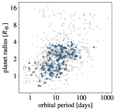
Figure 1: Planetary radius and orbital period, for all the known transiting planets associated with the 153 planet hosts in our sample.

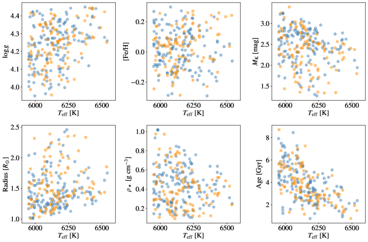
Figure 2: Comparison between the properties of the planet hosts (blue) and control stars (red). The precision of the measurements of $T_{\rm eff}$, $\log g$, [Fe/H], and $v\sin i$ is 60 K, 0.10 dex, 0.04 dex, and 1.0 km s^-1, respectively. In the the upper right panel, the vertical coordinate is the absolute magnitude based on the 2MASS apparent magnitude $m_{K}$ and the Gaia DR2 parallax, with no allowance for extinction. The radius, mean density, and age are from fits to MIST isochrones, and have typical internal uncertainties of 3%, 6%, and 30%, respectively.

We used two-sided Kolmogorov-Smirnov tests to check on the “null hypothesis” that the planet hosts and control stars have spectroscopic parameters drawn from the same parent distribution. The null hypothesis cannot be ruled out for $T_{\rm eff}$ ($p=0.57$), $\log g$ ($p=0.99$), or [Fe/H] ($p=0.44$). Likewise, the Anderson-Darling test cannot reject the null hypothesis for any of those three parameters ($p=0.66$, 0.99, and 0.43, respectively).

The preceding tests did not find any differences in the distributions of individual parameters, but are not capable of checking for differences in the joint distribution of two parameters. For this, we performed the two-dimensional generalization of the Kolmogorov-Smirnov test described by Press & Teukolsky (1988), which they attributed to earlier work by Fasano & Franceschini (1987) and Peacock (1983). We tested the joint distributions of $(T_{\rm eff},\log g)$, $(T_{\rm eff},{\rm[Fe/H]})$, and $(\log g,{\rm[Fe/H]})$. In all three cases, the test result was compatible with the hypothesis that the parameters are drawn from the same joint distribution ($p>0.3$). While these tests are only 2-d and not 3-d, and share the same shortcomings as the original KS test (see, e.g., Feigelson & Babu, 2012), they give us some confidence that the control stars are similar to the planet hosts.

Figure 2 shows the distributions of the spectroscopic parameters and other parameters of interest. This includes the $K$-band absolute magnitude, computed from the 2MASS apparent magnitude (Cutri et al., 2003) and the Gaia parallax (Gaia Collaboration et al., 2018) without any correction for extinction. The other parameters depicted are the mass, radius, mean density, and age of the stars, based on fitting the spectroscopic parameters to the MIST stellar-evolutionary models (Choi et al., 2016), using the method described by Fulton & Petigura (2018).

4 Model-Independent Tests

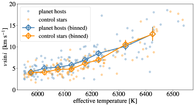
Figure 3: Measurements of projected rotation velocity versus effective temperature, for planet hosts (blue) and control stars (orange). The diamonds are binned values of $v\sin i$. For effective temperatures cooler than 6250 K, the planet hosts have higher mean values of $v\sin i$ than the control stars, indicating a tendency toward spin-orbit alignment.

Figure 3 shows the projected rotation velocity as a function of effective temperature, both for individual stars and for averages within temperature bins. The bins were chosen to have a width of 50 K for stars cooler than 6250 K, and 100 K for the less numerous hotter stars. For both samples, the average value of $v\sin i$ rises with $T_{\rm eff}$, as expected; this temperature range spans the well-known “Kraft break” above which stars are observed to rotate faster (Struve, 1930; Kraft, 1967). This trend is attributed to the reduced rate of magnetic braking for hot stars that lack thick outer convective envelopes.

It appears from Figure 3 that the relatively cool planet-hosting stars ($T_{\rm eff}<6250$ K) tend to have higher $v\sin i$ values than the control stars. This is a sign that these planet hosts have systematically higher values of $\sin i$ and therefore have low obliquities. We performed two statistical tests to quantify the difference in the $v\sin i$ distributions.

First, we performed the two-dimensional Kolmogorov-Smirnov test referenced earlier, using $T_{\rm eff}$ and $v\sin i$ as the two dimensions. The null hypothesis that the planet hosts and control stars have values of these two parameters drawn from the same joint distribution is assigned $p=0.028$. When applied only to the planet hosts and control stars with $T_{\rm eff}<6250$ K, the same test gives $p=0.0034$, representing a stronger rejection of the null hypothesis.

The second test was based on the observation that the planet hosts have a mean $v\sin i$ that exceeds that of the control stars in all of the first 6 temperature bins shown in Figure 3. How often would differences at this level occur by chance, if $T_{\rm eff}$ and $v\sin i$ for all the stars were drawn from the same two-dimensional distribution? We answered this question through a Monte Carlo procedure. We quantified the difference between the two distribution with the statistic

$$S\equiv\sum_{n=1}^{8}\frac{\langle v\sin i\rangle_{{\rm p},n}-\langle v\sin i\rangle_{{\rm c},n}}{\sqrt{\sigma^{2}_{{\rm p},n}+\sigma^{2}_{{\rm c},n}}},$$ (2)

where $\langle v\sin i\rangle_{n}$ is the mean value $v\sin i$ within the $n$th temperature bin; $\sigma_{n}$ is the corresponding standard deviation of the mean; and “p” and ”c” refer to the planet sample and the control sample, respectively. The real data have $S_{\rm obs}=8.3$. To create simulated data sets, we combined the 150 planet hosts and 101 control stars to form a combined sample of 251 stars, and then randomly drew (with replacement) 150 members of the combined sample to serve as “planet hosts” and 101 members to serve as “control stars.” By construction, the simulated data sets have parameters that are drawn from the same joint distribution. We computed the $S$ statistic for each of $10^{5}$ simulated data sets; in no case did we find $S>S_{\rm obs}$. Therefore, according to this test, $p<10^{5}$.

These model-independent tests confirmed the visual impression that the $v\sin i$ distributions of the planet hosts and control stars are significantly different, at least for the stars with $T_{\rm eff}<6250$ K. In the following sections, we use a simple model to quantify the resulting constraints on the obliquity distribution of the planet-hosting stars.

5 A Simple Model

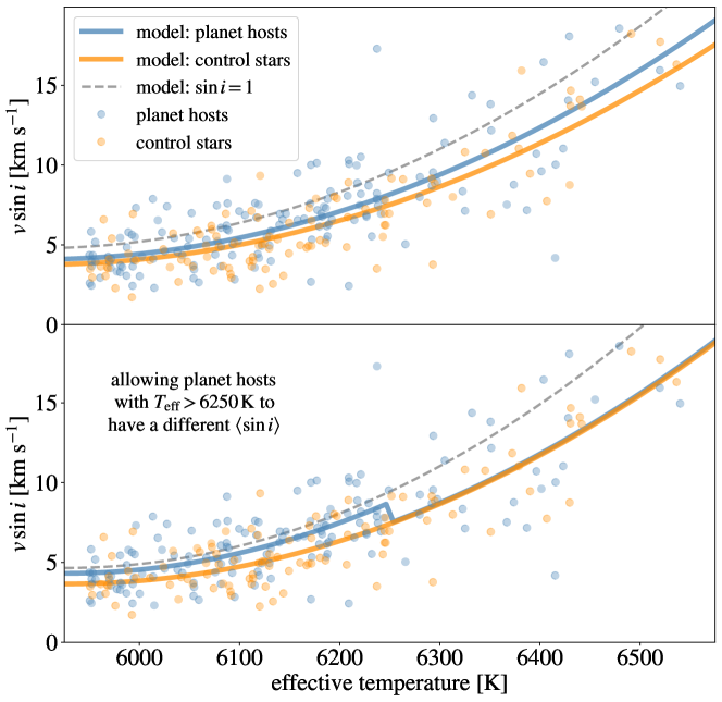
Figure 4: Measurements of projected rotation velocity versus effective temperature, for planet host (blue) and control stars (orange). The curves illustrate the best-fitting models. In the top panel, all the planet hosts are assumed to have the same value of $\langle\sin i\rangle$. In the bottom panel, the hosts cooler than 6250 K were allowed to have a different value of $\langle\sin i\rangle$ from the hosts hotter than 6250 K. In both panels, the gray dashed curve is the mean rotation velocity $\langle v\rangle$, the blue curve is $\langle v\rangle\langle\sin i\rangle$ fitted to the planet hosts, and the orange curve is $\langle v\rangle\times\pi/4$ fitted to the control stars.

5.1 Premises

Our model is based on the following premises:

1. A star’s rotation velocity $v$ and inclination $i$ are independent variables. This seems uncontroversial, since the rotation velocity is an intrinsic quantity, while the inclination depends on our arbitrary position within the galaxy.

2. For any value of the effective temperature, the control stars and the planet hosts have the same distribution of rotation velocities. This is justified by the sample construction and comparisons presented in Section 3.

3. The mean rotation velocity $\langle v\rangle$ is a quadratic function of effective temperature. This is a simplifying assumption based on the trend observed in Figure 3.

4. The measurements of $v\sin i$ for the control stars and the planet hosts are subject to the same systematic uncertainties. Ensuring this is the case was the motivation for obtaining all the spectra with the same instrument and analyzing them with the same code.

5. The control stars are randomly oriented in space.

To these, we add a sixth premise, and consider two different cases:

• The obliquities of the transiting planet hosts are all drawn from the same distribution.

• There are two different obliquity distributions: one for hosts cooler than 6250 K, and one for hosts hotter than 6250 K.

The second case is inspired by the appearance of Figure 3, as well as the fact that the obliquity distribution of hot Jupiter hosts has been observed to broaden as the temperature is increased past 6250 K, the approximate location of the Kraft break.

The only aspect of the obliquity distribution that is well constrained by the data is $\langle\sin i\rangle$, the mean value of $\sin i$ for the planet hosts. For this reason, our models include $\langle\sin i\rangle$ as a free parameter but do not adopt a particular functional form for the obliquity distribution. A population of randomly oriented stars would have $\langle\sin i\rangle=\pi/4\approx 0.785$, and a population of transiting-planet hosts with low obliquities would have $\langle\sin i\rangle\approx 1$.

We fitted a single model to all of the stars, both the planet hosts and the control stars. For all the stars, the mean rotation velocity in the model is

$$\langle v\rangle(\tau)=c_{0}+c_{1}\tau+c_{2}\tau^{2},$$ (3)

where

$$\tau\equiv\frac{T_{\rm eff}-6250\,{\rm K}}{300\,{\rm K}}$$ (4)

varies from $-1$ to $+1$, and $c_{0}$, $c_{1}$, and $c_{2}$ are free parameters. The mean $v\sin i$ value in the model depends on whether the star is a control star or a planet host:

$$\langle v\sin i\rangle_{n} = \langle v\rangle_{n}\times\frac{\pi}{4}~{}~{}({\rm control~{}stars})$$ (5)

$$\langle v\sin i\rangle_{n} = \langle v\rangle_{n}\times\langle\sin i\rangle~{}~{}({\rm planet~{}hosts}),$$ (6)

where we have used the fact that $v$ and $\sin i$ are uncorrelated. Thus, in this model, the polynomial coefficients are constrained by all of the stars, and the $\langle\sin i\rangle$ parameter is constrained by the planet hosts.

The goodness-of-fit statistic was taken to be

$$\chi^{2}=\sum_{n=1}^{251}\left(\frac{v\sin i_{{\rm obs},n}-\langle v\sin i\rangle_{{\rm calc},n}}{1\,{\rm km\,s}^{-1}}\right)^{2},$$ (7)

where $v\sin i_{{\rm obs},j}$ is the observed value of $v\sin i$ of the $n$th star, $\langle v\sin i\rangle_{{\rm calc},i}$ is the mean value of $v\sin i$ calculated according to the model, and $1\,{\rm km\,s}^{-1}$ is the measurement uncertainty.

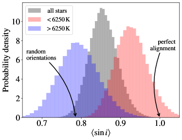
Figure 5: Posterior probability distributions for $\langle\sin i\rangle$, marginalized over all other parameter values. The gray curve shows the case in which the obliquities of all the planet hosts were assumed to be drawn from the same distribution. The red and blue curves shows the case in which the stars with $T_{\rm eff}<6250$ K were allowed to have a different obliquity distribution from the stars with $T_{\rm eff}>6250$ K.

5.2 Results

For the case of a single obliquity distribution (premise 5a), the best-fitting model has $\langle\sin i\rangle=0.856$ and $\chi^{2}_{\rm min}=935$, with 247 degrees of freedom (251 data points and 4 free parameters). The model does not fit the data points to within the measurement uncertainties, nor should we expect it to fit so well. An individual measurement of $v\sin i$ departs from the calculated $\langle v\sin i\rangle$ not only because of the measurement uncertainty, but also because of the intrinsic dispersion in the rotation velocities and the dispersion in $\sin i$. These deviations are drawn from different distributions, neither of which is known well. For this reason, we used a bootstrap procedure to establish the confidence intervals for the model parameters.

We created $10^{5}$ simulated data sets, each with the same number of planet hosts and control stars as the real data set, by drawing data points randomly (with repetitions allowed) from the real data. The model was fitted to each simulated data set by minimizing the $\chi^{2}$ statistic. The resulting collection of $10^{5}$ parameter sets was interpreted as a sampling from the joint probability density of the parameter values.

For the case of a single obliquity distribution (premise 6a), the bootstrap procedure gave $\langle\sin i\rangle=0.856\pm 0.036$, where the uncertainty interval encompasses 68% of the bootstrap simulation results. For the case of two different obliquity distributions (premise 6b), the stars cooler than 6250 K have $\langle\sin i\rangle=0.928\pm 0.042$. The higher value obtained in this case implies a stronger tendency toward spin-orbit alignment; indeed, the result differs by only 1.7-$\sigma$ from the condition of perfect alignment. Conversely, the stars hotter than 6250 K have $\langle\sin i\rangle=0.794\pm 0.052$, which is consistent with random orientations ($\pi/4\approx 0.785$). Table 1 gives the results for all the parameters. Figure 4 show the best-fitting model curves, and Figure 5 shows the probability distributions for the key parameters.

Table 1: Parameter values.

Parameter	Single obliquity	Two obliquity
value	distribution	distributions
$\langle\sin i\rangle$	$0.856\pm 0.036$	$0.928\pm 0.042$, $<$6250 K
		$0.794\pm 0.052$, $>$6250 K
$c_{0}$	$9.57\pm 0.29$	$9.44\pm 0.28$
$c_{1}$	$8.01\pm 0.54$	$8.87\pm 0.61$
$c_{2}$	$3.30\pm 0.62$	$4.05\pm 0.62$

5.3 von-Mises Fisher distribution

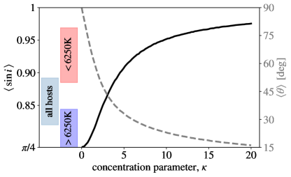
Figure 6: Relationship between the concentration parameter $\kappa$ of the von-Mises Fisher distribution and the mean values of $\sin i$ (solid black line, left-side axis) and obliquity (gray dashed line, right-side axis). On the left, the colored bars indicate the 1-$\sigma$ allowed ranges of $\langle\sin i\rangle$ for the planet hosts, using the model described in Section 5.

Further steps are needed to obtain quantitative constraints on the obliquity distribution, because $\sin i$ is only one aspect of the obliquity. The other aspect is the position angle $\Omega$ of the projection of the spin axis onto the orbital plane. The relationship is

$$\sin i=\sqrt{1-\sin^{2}\theta\cos^{2}\Omega}.$$ (8)

Even though our model is not committed to a specific shape for the obliquity distribution, we find it useful to interpret the results with reference to a von-Mises Fisher (vMF) distribution,

$$p(\hat{n}_{\star})\propto\exp(\kappa\hat{n}_{\star}\!\mathbin{\mathchoice{\hbox to5.74991pt{\hfil\raise 0.0pt\hbox{\scalebox{0.5}{\lower 0.0pt\hbox{$\displaystyle\bullet$}}}\hfil}}{\hbox to5.74991pt{\hfil\raise 0.0pt\hbox{\scalebox{0.5}{\lower 0.0pt\hbox{$\textstyle\bullet$}}}\hfil}}{\hbox to4.79156pt{\hfil\raise 0.0pt\hbox{\scalebox{0.5}{\lower 0.0pt\hbox{$\scriptstyle\bullet$}}}\hfil}}{\hbox to4.15268pt{\hfil\raise 0.0pt\hbox{\scalebox{0.5}{\lower 0.0pt\hbox{$\scriptscriptstyle\bullet$}}}\hfil}}}\!\,\hat{n}_{\rm o}),$$ (9)

where $\hat{n}_{\star}$ and $\hat{n}_{\rm o}$ are the unit vectors in the directions of the spin axis and the orbital axis, respectively, and the obliquity $\theta$ is equal to $\cos^{-1}(\hat{n}_{\star}\mathbin{\mathchoice{\hbox to5.74991pt{\hfil\raise 0.0pt\hbox{\scalebox{0.5}{\lower 0.0pt\hbox{$\displaystyle\bullet$}}}\hfil}}{\hbox to5.74991pt{\hfil\raise 0.0pt\hbox{\scalebox{0.5}{\lower 0.0pt\hbox{$\textstyle\bullet$}}}\hfil}}{\hbox to4.79156pt{\hfil\raise 0.0pt\hbox{\scalebox{0.5}{\lower 0.0pt\hbox{$\scriptstyle\bullet$}}}\hfil}}{\hbox to4.15268pt{\hfil\raise 0.0pt\hbox{\scalebox{0.5}{\lower 0.0pt\hbox{$\scriptscriptstyle\bullet$}}}\hfil}}}\hat{n}_{\rm o})$. The vMF distribution is a widely-used model in directional statistics that resembles a two-dimensional Gaussian distribution wrapped around a sphere. Just as the Gaussian distribution has the maximum entropy for a given variance, the vMF distribution has the maximum entropy for a fixed value of the mean obliquity (Mardia, 1975). As $\kappa\rightarrow 0$, the distribution becomes isotropic, and as $\kappa\rightarrow\infty$, it approaches a delta-function centered on $\hat{n}_{\rm o}$.

We numerically computed the relationship between $\kappa$ and the mean obliquity $\langle\theta\rangle$, as well as $\langle\sin i\rangle$, assuming that $\Omega$ is uniformly distributed between $0^{\circ}$ and $360^{\circ}$. The results are shown in Figure 6, along with the constraints on $\langle\theta\rangle$ obtained from our best-fitting models of the data. When all of the planet hosts are modeled together (premise 5a), the 1-$\sigma$ allowed range for $\kappa$ is from 1.7 to 4.2, and the mean obliquity ranges from 37 to 58 degrees. When the planet hosts are divided into two samples according to effective temperature (premise 5b), the stars cooler than 6250 K have 1-$\sigma$ ranges of $\kappa=3.8$-16 and $\langle\theta\rangle=18$-38 degrees, while the ranges for the hotter stars are $\kappa=0$-2.3 and $\langle\theta\rangle=49$-88 degrees.

These results can be compared to previous inferences of $\kappa$ from different techniques and different samples of planet-hosting stars. Fabrycky & Winn (2009) found $\kappa>7.6$ (95% conf.) based on the first 11 observations of the Rossiter-McLaughlin effect, all of which were hot Jupiter hosts. Since that time, many more misaligned hot Jupiters have been found; a more up-to-date analysis by Muñoz & Perets (2018) gave $\kappa=2.2_{-0.6}^{+0.2}$. This is comparable to the obliquity distribution of the hotter half of the stars in our sample, while the cooler half of the stars have a greater tendency to be well-aligned.

Previous inferences of the obliquity distribution of Kepler stars have mainly focused on the subset of stars with detected rotation periods. Such samples may be suffer from biases related to orientation and transiting planet detection, as noted in the Introduction. Nevertheless, in practice, our results are in agreement with the prior results. Since the stars in the previous studies were almost all cooler than $6250$ K, the appropriate comparison is to cooler half of our sample, for which we obtained $\kappa=3.8$-16. Morton & Winn (2014) analyzed 70 Kepler stars, finding $\kappa=19_{-12}^{+73}$ for stars with multiple transiting planets, and $4.8_{-1.6}^{+2.0}$ for stars with only one detected transiting planet. To these results, Campante et al. (2016) added asteroseismic determinations of $\sin i$ for 25 Kepler stars, finding $\kappa=11.5_{-5.7}^{+7.5}$ for the entire sample. Winn et al. (2017) expanded the work by Morton & Winn (2014) to include 156 stars and found $\kappa\gtrsim 5$ regardless of transit multiplicity. Likewise, Muñoz & Perets (2018) analyzed a sample of 257 cool Kepler stars, and found $\kappa=14.5_{-6}^{+13.5}$. All of the confidence intervals of these previous studies overlap with ours, although in many cases the intervals are large.

5.4 Model validation

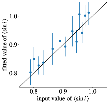
Figure 7: Results of applying our modeling procedure to simulated data with different assumed values of $\langle\sin i\rangle$, as described in Section 5.4. The fitted values and uncertainties are consistent with the input values across the range of possible values.

To validate our modeling procedure, we fitted simulated data sets. We generated simulated data sets with different input values of $\langle\sin i\rangle$, and used our modeling procedure to “recover” the best-fitting value of $\langle\sin i\rangle$ and test for agreement. Each simulated data set was created as follows. The 101 control stars were assigned random orientations, and the 151 planet hosts were assigned fictitious obliquities drawn from a vMF distribution. For all the stars, a fictitious position angle was drawn from a uniform distribution. We assumed a quadratic relationship between $\langle v\rangle$ and $T_{\rm eff}$ based on the best-fitting model to the real data. Then, we assigned a $v\sin i$ value to each star:

$$v\sin i=\langle v\rangle(1+0.2x_{1})\sin i+(1\,{\rm km\,s}^{-1})x_{2},$$ (10)

where $x_{1}$ and $x_{2}$ are independent random draws from a standard normal distribution $\mathcal{N}(0,1)$, to account for the intrinsic dispersion of rotation velocities (assumed to be 20%) and the measurement uncertainty, respectively.

Simulated data sets were created based on values of $\kappa$ ranging from 0 to 40, corresponding to nearly the full range of possible values of $\langle\sin i\rangle$. We fitted the simulated data sets using the same code that was used on the actual data. Figure 7 shows the results: the recovered values of $\langle\sin i\rangle$ agree with the input values to within the reported uncertainties, providing support for the validity of our procedure.

6 Discussion

Overall, the Kepler planet-hosting stars of spectral types from early-G to late-F have systematically higher values of the projected rotation velocity than similar stars chosen without regard to planets or spin-axis orientation. Although this trend had been seen by Winn et al. (2017) and Muñoz & Perets (2018), the improved control sample makes it possible to be more confident in quantitative comparisons. To explain the difference in terms of geometry, the obliquity distribution of the planet hosts must be intermediate between the limiting cases of perfect alignment and random directions.

We analyzed the data using simple models for the obliquity distribution, and presented evidence that the hottest stars in the sample have a broader distribution than the less hot stars. Regardless of the details, the important point is that many of the stars in our sample (especially the late-F stars) appear to have larger obliquities than the Sun. This has been known for a decade for the hosts of hot Jupiters, but to this point it has not been clear that it is also generally true of the hosts of other types of planets.

A key assumption in our study is that the rotation velocities of the planet hosts and control stars are drawn from the same distribution. We tried to ensure this is the case through careful matching of observable spectroscopic parameters. Still, it remains possible that systematic differences exist. In principle, the control stars, being situated in a different and more nearby location in the Galaxy, may have systematically different rotation velocities than the planet hosts even for fixed values of the spectroscopic parameters, due to subtle differences in chemical composition or formation history. There might also be physical processes specific to the formation and evolution of Kepler-type planets that alter a star’s rotational history. Tidal interactions with the known planets are generally too weak to affect the star’s rotation, but one might speculate about previously ingested planets, or differing magnetic and accretion histories. Any such differences would be muted, though, by the fact that between one-third and one-half of the control stars also have Kepler-type planets that do not happen to be transiting.

Despite these caveats, our conclusions are supported by two complementary lines of evidence. The first is the work by Mazeh et al. (2015), noted in Section 1. They studied the obliquities of Kepler stars using photometric variability data. Stronger variability is expected for stars viewed at high inclination, the perspective that allows spots and plages to rotate into and out of view. Therefore, if the transiting-planet hosts have low obliquities, they should show stronger variability than a sample of randomly-oriented stars, whereas for random obliquities, the planet hosts would show the same level of variability as the randomly-oriented stars. For stars cooler than about 6000 K, Mazeh et al. (2015) found the planet hosts to show stronger variability than stars without detected transiting planets, by approximately the factor of $4/\pi\approx 1.3$ that is expected if the planet hosts have low obliquities and the other stars are randomly oriented.

They also found that this trend reverses for the hotter stars: the planet hosts display weaker variability than the randomly-oriented stars, with an amplitude ratio of 0.6. This was surprising, because even in the seemingly extreme case in which the planet hosts are randomly oriented, the amplitude ratio would be 1.0. For this ratio to fall below unity due only to differences in viewing angles, we would be led to the unexpected conclusion that the obliquities of the hot stars are preferentially near 90^∘.

However, Mazeh et al. (2015) found that at least part of the difference between the variability levels of the hot planet hosts and the randomly-oriented stars is due to a selection effect. Namely, transiting planets are more readily detected around stars with intrinsically lower levels of photometric variability. Simulations of this selection effect showed that it was indeed significant, but not large enough to have reduced an intrinsic amplitude ratio of 1.3 all the way down to the observed ratio of 0.6. Thus, this study left open the possibility that the hot Kepler stars have a broader obliquity distribution than the cool stars, an interpretation that harmonizes with our findings.

The second line of evidence for high obliquities among hot stars with planets other than hot Jupiters comes from recent observations of individual systems. We are aware of only two obliquity measurements for stars with effective temperatures between 5900 K and 6450 K that do not involve hot Jupiters, and in both cases, the obliquity is high. The first case is Kepler-408 ($T_{\rm eff}=6088$ K), which has an Earth-sized planet in a 2.5-day orbit. Asteroseismology revealed that the obliquity is approximately 45^∘ (Kamiaka et al., 2019). The second case is K2-290 ($T_{\rm eff}=6302$ K), which has a 3 $R_{\oplus}$ planet in a 9.2-day orbit and a Jupiter-sized planet in a 48-day orbit. Observations of the Rossiter-McLaughlin effect show that the star’s rotation is retrograde (Hjorth et al., submitted). Another relevant case is Kepler-56 (Huber et al., 2013), which has two planets of sizes 6.5 and 9.8 $R_{\oplus}$ and orbital periods of 10.5 and 21 days. The host star is a subgiant with a mass of 1.3 $M_{\odot}$ and an effective temperature of 4840 K, although it was probably about 6400 K when it was on the main sequence. The stellar obliquity is at least 45^∘, based on an asteroseismic analysis. Some day we may accumulate enough of these individual measurements to measure the obliquity distribution more directly.

While this is not the place to evaluate specific theories in detail, we can list the previously published theories for obliquity excitation that have the desired property that they do not require the presence of a close-orbiting giant planet:
$\bullet$ A misalignment between the protoplanetary disk due to inhomogeneities in the molecular cloud (Bate et al., 2010; Fielding et al., 2015; Takaishi et al., 2020), magnetic interactions (Lai et al., 2011), or a companion star (Batygin, 2012; Spalding & Batygin, 2015; Zanazzi & Lai, 2018).
$\bullet$ Ongoing nodal precession driven by a stellar companion or wide-orbiting giant planet on a highly inclined orbit (Anderson & Lai, 2018).
$\bullet$ A resonance between the nodal precession rates of an inner planet and an outer planet that occurs during the dissipation of the protoplanetary disk (Petrovich et al., 2020).
$\bullet$ Random tumbling of the spin-axis orientation of the photosphere due to stochastic internal gravity waves (Rogers et al., 2012).

Another desired property is that cooler stars with small planets should have low obliquities. The dividing line of about $6250$ K is significant in stellar-evolutionary theory because the hot stars have thin or absent outer convective zones, leading to weaker or absent magnetic braking, more rapid rotation, and weaker tidal dissipation. Thus, it seems likely that a successful theory will involve these distinctions. At least two of the theories listed above make an explicit distinction between cool and hot stars: those of Rogers et al. (2012) (which pertains only to hot stars) and Spalding & Batygin (2015) (which appeals to the weaker magnetic field of hot stars). Of course, obliquities might be excited and damped by different mechanisms in different situations, including some that theoreticians have not yet identified.

Table 2: Spectroscopic properties of the planet hosts.

KIC no.	KOI no.	$T_{\mathrm{eff}}$ [K]	$\log g$	[Fe/H]	$v\sin i$ [km s-1]
1724719	4212	6215	4.35	$0.14$	6.56
1871056	1001	6298	4.15	$0.14$	8.97
1996180	2534	6118	4.36	$0.02$	4.43
2142522	2403	6186	4.37	$0.18$	5.34
2307415	2053	6183	4.27	$0.08$	6.77
2854914	1113	6099	4.27	$0.04$	5.24
2989404	1824	5987	4.35	$-0.16$	3.07
3114811	1117	6401	4.12	$-0.05$	9.61
3120904	3277	5997	3.95	$-0.02$	7.33
3447722	1198	6323	4.39	$0.10$	8.36
3632418	975	6186	4.08	$-0.05$	7.31
3642289	301	5995	4.10	$-0.08$	5.51
3656121	386	5983	4.40	$0.06$	3.60
3661886	2279	5950	4.25	$0.05$	2.60
3867615	2289	6048	4.28	$0.09$	4.90
3939150	1215	6054	4.02	$0.09$	2.90
3964109	393	6280	4.34	$-0.19$	7.99
3969687	2904	6077	3.96	$0.30$	7.47
4242692	3928	6192	4.31	$-0.05$	6.59
4278221	1615	6013	4.43	$0.22$	7.88
4349452	244	6280	4.31	$-0.03$	9.25
4478168	626	6131	4.33	$-0.17$	3.99
4563268	627	6050	4.18	$0.18$	5.39
4656049	629	6059	4.34	$-0.29$	2.65
4741126	1534	6208	4.29	$0.04$	8.07
4833421	232	5994	4.25	$-0.06$	4.03
4914566	2635	6052	4.09	$-0.14$	6.99
5120087	639	6184	4.34	$0.05$	7.39
5175024	2563	6119	4.00	$0.11$	7.53
5183357	1669	6140	4.24	$-0.05$	6.94
5281113	4411	6119	4.44	$-0.14$	4.18
5350244	2555	6180	4.38	$-0.07$	6.14
5384079	2011	6455	4.44	$-0.02$	15.21
5514383	257	6220	4.36	$0.12$	7.49
5561278	1621	6089	4.06	$0.02$	5.90
5613330	649	6244	4.10	$0.22$	7.80
5631630	2010	6416	4.27	$-0.00$	10.03
5866724	85	6229	4.22	$0.15$	8.71
5880320	1060	6351	4.16	$-0.29$	12.17
5966154	655	6171	4.25	$-0.02$	2.69
6026924	4276	6221	4.00	$0.12$	8.20
6105462	2098	6305	4.33	$-0.13$	11.39
6125481	659	6374	4.45	$-0.03$	8.77
6196457	285	5952	4.03	$0.20$	3.96
6206214	2252	6116	4.02	$0.08$	7.61
6269070	2608	6429	4.40	$0.06$	18.06
6289257	307	6035	4.41	$-0.08$	5.44
6310636	1688	5993	4.08	$0.18$	5.64
6345732	2857	6189	4.15	$0.24$	6.28
6442377	176	6423	4.44	$-0.19$	11.03
6599975	3438	6054	4.38	$-0.14$	3.72
6716545	2906	6087	4.15	$-0.28$	5.98
6937529	4382	6217	4.24	$-0.12$	9.98
7040629	671	6093	4.24	$0.03$	5.06
7133294	4473	5952	4.00	$0.04$	5.83
7175184	369	6227	4.37	$-0.12$	6.86
7215603	1618	6209	4.16	$0.13$	10.07
7219825	238	6131	4.27	$-0.10$	5.88
7259298	2561	6014	4.16	$0.04$	4.12
7375348	266	6232	4.42	$-0.02$	5.53
7673192	2722	6140	4.38	$-0.07$	6.26
7755636	1921	6479	4.33	$0.04$	18.56
7831264	171	6237	4.30	$0.10$	7.88
8013439	2352	6387	4.29	$-0.14$	7.17
8073705	3245	6115	4.31	$-0.10$	3.57
8077137	274	6081	4.09	$-0.04$	6.07
8081187	1951	6093	4.33	$-0.20$	4.35
8121310	317	6520	4.28	$0.05$	15.94
8158127	1015	5950	4.16	$-0.10$	4.37
8161561	688	6218	4.27	$-0.06$	8.88
8193178	572	6003	4.16	$-0.06$	4.28
8212002	2593	6238	4.28	$0.22$	7.46
8292840	260	6292	4.34	$-0.16$	8.71
8394721	152	6428	4.39	$0.07$	14.05
8410727	1148	6127	4.27	$0.16$	5.51
8494142	370	6117	4.09	$0.07$	6.71
8636434	3946	6325	4.26	$-0.22$	7.13
8644365	3384	5956	4.18	$0.05$	3.94
8738735	693	6018	4.08	$-0.03$	6.54
8751796	3125	6293	4.32	$-0.11$	9.55
8773015	4301	6266	4.44	$-0.14$	5.04
8822366	1282	6087	4.16	$-0.13$	6.22
8883329	2595	6332	4.30	$0.04$	14.37
8972058	159	6055	4.40	$-0.01$	3.46
9009036	4585	6158	4.18	$-0.11$	9.50
9015738	1616	6067	4.29	$0.18$	5.32
9026749	2564	6087	4.03	$-0.13$	9.13
9070666	3008	5981	4.07	$-0.08$	5.44
9277896	1632	6088	4.16	$0.02$	7.60
9412623	4640	6396	4.28	$-0.06$	10.71
9450647	110	6241	4.38	$-0.16$	6.95
9451706	271	6158	4.23	$0.27$	6.56
9458613	707	5953	4.07	$0.14$	4.36
9466429	2786	6367	4.25	$-0.13$	7.52
9467404	2717	6025	4.25	$-0.02$	4.61
9529744	1806	6146	4.27	$-0.05$	6.94
9530945	708	6100	4.19	$-0.10$	7.11
9549648	1886	6221	4.18	$0.05$	10.52
9579641	115	5961	4.39	$-0.08$	2.94
9590976	710	6540	4.26	$-0.06$	14.96
9649706	2049	5972	4.15	$0.07$	4.14
9696358	2545	6105	3.99	$0.14$	6.86
9717943	2273	6038	4.25	$0.25$	4.55
9763348	1852	6415	4.35	$-0.17$	4.18
9782691	590	5981	4.42	$-0.00$	3.72
9881662	327	6043	4.28	$-0.02$	4.35
9886361	2732	6082	4.07	$0.08$	4.90
9892816	1955	6249	4.25	$0.09$	9.52
9904006	2135	6171	4.20	$0.05$	7.60
9965439	722	6188	4.38	$-0.11$	5.54
10227020	730	5952	4.19	$0.27$	2.45
10253547	2153	6023	4.19	$-0.06$	5.79
10337258	333	6237	4.41	$0.11$	8.23
10460984	474	5981	4.42	$0.02$	3.28
10471515	2961	6078	4.27	$0.13$	5.24
10615440	4765	6227	4.31	$0.15$	6.76
10916600	2623	6178	4.10	$0.13$	7.18
10963065	1612	6095	4.27	$-0.14$	2.83
11019987	3060	6187	4.10	$-0.06$	6.17
11043167	1444	6191	4.11	$0.10$	8.35
11086270	124	5977	4.27	$-0.10$	3.33
11121752	2333	6081	4.35	$-0.15$	3.66
11127479	2792	5969	4.17	$0.21$	4.26
11133306	276	5993	4.34	$-0.01$	2.43
11259686	294	6076	4.36	$0.05$	4.39
11336883	1445	6351	4.26	$0.14$	13.81
11337566	2632	6209	4.07	$-0.02$	10.31
11342416	2366	6165	4.31	$0.01$	6.64
11401755	277	5987	4.13	$-0.19$	4.84
11401767	2195	6130	4.24	$-0.12$	4.96
11442793	351	5993	4.24	$0.09$	3.64
11457726	2047	6172	4.37	$-0.02$	5.33
11460462	2110	6404	4.28	$0.23$	16.45
11499228	2109	6028	4.07	$0.04$	7.41
11560897	2365	5952	4.17	$0.21$	3.66
11572193	3109	6237	4.05	$0.09$	17.29
11621223	355	6122	4.25	$0.20$	4.94
11656246	1532	6143	4.21	$0.15$	6.59
11666881	167	6209	4.15	$0.04$	2.43
11807274	262	6171	4.18	$-0.09$	10.01
11811193	2260	6188	4.22	$0.01$	7.88
11905011	297	6181	4.31	$0.12$	6.96
12024120	265	6015	4.18	$0.14$	2.31
12058931	546	5971	4.24	$0.12$	3.55
12120484	2407	5956	4.12	$0.19$	5.19
12206313	2714	5989	4.02	$-0.02$	5.79
12254909	2372	5970	4.17	$-0.09$	3.92
12314973	279	6294	4.27	$0.18$	12.93
12416661	3122	6177	4.01	$0.23$	10.13
12600735	548	6000	4.23	$-0.06$

Note. — The uncertainties in $T_{\mathrm{eff}}$, $\log g$, [Fe/H], and $v\sin i$ are 60 K, 0.1, 0.1, and 1 km s^-1, respectively.

Table 3: Spectroscopic properties of the control stars.

Note. — The uncertainties in $T_{\mathrm{eff}}$, $\log g$, [Fe/H], and $v\sin i$ are 60 K, 0.1, 0.1, and 1 km/s, respectively.

References

- Anderson & Lai (2018) Anderson, K. R., & Lai, D. 2018, MNRAS, 480, 1402, doi: 10.1093/mnras/sty1937
- Bate et al. (2010) Bate, M. R., Lodato, G., & Pringle, J. E. 2010, MNRAS, 401, 1505, doi: 10.1111/j.1365-2966.2009.15773.x
- Batygin (2012) Batygin, K. 2012, Nature, 491, 418, doi: 10.1038/nature11560
- Borucki (2017) Borucki, W. J. 2017, Proceedings of the American Philosophical Society, 161, 38
- Campante et al. (2016) Campante, T. L., Lund, M. N., Kuszlewicz, J. S., et al. 2016, ApJ, 819, 85, doi: 10.3847/0004-637X/819/1/85
- Choi et al. (2016) Choi, J., Dotter, A., Conroy, C., et al. 2016, ApJ, 823, 102, doi: 10.3847/0004-637X/823/2/102
- Cutri et al. (2003) Cutri, R. M., Skrutskie, M. F., van Dyk, S., et al. 2003, 2MASS All Sky Catalog of point sources.
- Dawson (2014) Dawson, R. I. 2014, ApJ, 790, L31, doi: 10.1088/2041-8205/790/2/L31
- Fabrycky & Winn (2009) Fabrycky, D. C., & Winn, J. N. 2009, ApJ, 696, 1230, doi: 10.1088/0004-637X/696/2/1230
- Fasano & Franceschini (1987) Fasano, G., & Franceschini, A. 1987, MNRAS, 225, 155, doi: 10.1093/mnras/225.1.155
- Feigelson & Babu (2012) Feigelson, E. D., & Babu, G. J. 2012, Modern Statistical Methods for Astronomy
- Fielding et al. (2015) Fielding, D. B., McKee, C. F., Socrates, A., Cunningham, A. J., & Klein, R. I. 2015, MNRAS, 450, 3306, doi: 10.1093/mnras/stv836
- Fulton & Petigura (2018) Fulton, B. J., & Petigura, E. A. 2018, AJ, 156, 264, doi: 10.3847/1538-3881/aae828
- Gaia Collaboration et al. (2018) Gaia Collaboration, Brown, A. G. A., Vallenari, A., et al. 2018, A&A, 616, A1, doi: 10.1051/0004-6361/201833051
- Huber et al. (2013) Huber, D., Carter, J. A., Barbieri, M., et al. 2013, Science, 342, 331, doi: 10.1126/science.1242066
- Johnson et al. (2017) Johnson, J. A., Petigura, E. A., Fulton, B. J., et al. 2017, AJ, 154, 108, doi: 10.3847/1538-3881/aa80e7
- Kamiaka et al. (2019) Kamiaka, S., Benomar, O., Suto, Y., et al. 2019, AJ, 157, 137, doi: 10.3847/1538-3881/ab04a9
- Kraft (1967) Kraft, R. P. 1967, ApJ, 150, 551, doi: 10.1086/149359
- Lai et al. (2011) Lai, D., Foucart, F., & Lin, D. N. C. 2011, MNRAS, 412, 2790, doi: 10.1111/j.1365-2966.2010.18127.x
- Mardia (1975) Mardia, K. V. 1975, Journal of the Royal Statistical Society. Series B (Methodological), 37, 349. http://www.jstor.org/stable/2984782
- Mazeh et al. (2015) Mazeh, T., Perets, H. B., McQuillan, A., & Goldstein, E. S. 2015, ApJ, 801, 3, doi: 10.1088/0004-637X/801/1/3
- Morton & Winn (2014) Morton, T. D., & Winn, J. N. 2014, ApJ, 796, 47, doi: 10.1088/0004-637X/796/1/47
- Muñoz & Perets (2018) Muñoz, D. J., & Perets, H. B. 2018, AJ, 156, 253, doi: 10.3847/1538-3881/aae7d0
- Peacock (1983) Peacock, J. A. 1983, MNRAS, 202, 615, doi: 10.1093/mnras/202.3.615
- Petigura (2015) Petigura, E. A. 2015, PhD thesis, University of California, Berkeley
- Petigura et al. (2017) Petigura, E. A., Howard, A. W., Marcy, G. W., et al. 2017, AJ, 154, 107, doi: 10.3847/1538-3881/aa80de
- Petrovich et al. (2020) Petrovich, C., Muñoz, D. J., Kratter, K. M., & Malhotra, R. 2020, ApJ, 902, L5, doi: 10.3847/2041-8213/abb952
- Press & Teukolsky (1988) Press, W. H., & Teukolsky, S. A. 1988, Computers in Physics, 2, 74, doi: 10.1063/1.4822753
- Ren et al. (2016) Ren, A., Fu, J., De Cat, P., et al. 2016, ApJS, 225, 28, doi: 10.3847/0067-0049/225/2/28
- Rogers et al. (2012) Rogers, T. M., Lin, D. N. C., & Lau, H. H. B. 2012, ApJ, 758, L6, doi: 10.1088/2041-8205/758/1/L6
- Schlaufman (2010) Schlaufman, K. C. 2010, ApJ, 719, 602, doi: 10.1088/0004-637X/719/1/602
- Spalding & Batygin (2015) Spalding, C., & Batygin, K. 2015, ApJ, 811, 82, doi: 10.1088/0004-637X/811/2/82
- Struve (1930) Struve, O. 1930, ApJ, 72, 1, doi: 10.1086/143256
- Takaishi et al. (2020) Takaishi, D., Tsukamoto, Y., & Suto, Y. 2020, MNRAS, 492, 5641, doi: 10.1093/mnras/staa179
- Thompson et al. (2018) Thompson, S. E., Coughlin, J. L., Hoffman, K., et al. 2018, ApJS, 235, 38, doi: 10.3847/1538-4365/aab4f9
- Triaud (2018) Triaud, A. H. M. J. 2018, The Rossiter-McLaughlin Effect in Exoplanet Research, 2, doi: 10.1007/978-3-319-55333-7_2
- Winn et al. (2010) Winn, J. N., Fabrycky, D., Albrecht, S., & Johnson, J. A. 2010, ApJ, 718, L145, doi: 10.1088/2041-8205/718/2/L145
- Winn & Fabrycky (2015) Winn, J. N., & Fabrycky, D. C. 2015, ARA&A, 53, 409, doi: 10.1146/annurev-astro-082214-122246
- Winn et al. (2017) Winn, J. N., Petigura, E. A., Morton, T. D., et al. 2017, AJ, 154, 270, doi: 10.3847/1538-3881/aa93e3
- Zanazzi & Lai (2018) Zanazzi, J. J., & Lai, D. 2018, MNRAS, 478, 835, doi: 10.1093/mnras/sty1075