The Exomoon Corridor: Half of all exomoons exhibit TTV frequencies within a narrow window due to aliasing

Abstract

Exomoons are expected to produce potentially detectable transit timing variations (TTVs) upon their parent planet. Unfortunately, distinguishing moon-induced TTVs from other sources, in particular planet-planet interactions, has severely impeded its usefulness as a tool for identifying exomoon candidates. A key feature of exomoon TTVs is that they will always be undersampled, due to the simple fact that we can only observe the TTVs once per transit/planetary period. We show that it is possible to analytically express the aliased TTV periodicity as a function of planet and moon period. Further, we show that inverting an aliased TTV period back to a true moon period is fraught with hundreds of harmonic modes. However, a unique aspect of these TTV aliases is that they are predicted to occur at consistently short periods, irrespective of what model one assumes for the underlying moon population. Specifically, 50% of all exomoons are expected to induce TTVs with a period between 2 to 4 cycles, a range that planet-planet interactions rarely manifest at. This provides an exciting and simple tool for quickly identifying exomoons candidates and brings the TTV method back to the fore as an exomoon hunting strategy. Applying this method to the candidate, Kepler-1625b i, reveals that its TTV periodicity centers around the median period expected for exomoons.

1 Introduction

One of the first methods proposed to look for moons of extrasolar planets, exomoons, is through transit timing variations (TTVs; Sartoretti & Schneider 1999). The amplitude of these variations is proportional to satellite-to-planet mass ratio, $(M_{S}/M_{P})$, multiplied by the moon’s semi-major axis ($a_{S}$), and can anywhere from less than a second to up to an hour (Kipping & Teachey, 2020).

Unfortunately, the detection of such signals is frustrated by two major obstacles. First, planet-planet interactions are a frequent source of TTVs (e.g. Holman et al. 2010; Nesvorný et al. 2014; Hadden & Lithwick 2017), making it difficult to assess whether a given TTV signal is truly caused by a satellite (e.g. see Szabó et al. 2013; Kipping et al. 2014). Second, any satellite orbiting within the Hill sphere will have an orbital period much shorter than the planetary period - which represents the sampling rate via transits. Accordingly, the signal is undersampled, as first proved in Kipping (2009a). A key conclusion of that work was that “the period of the exomoon cannot be reliably determined from TTVs, only a set of harmonic frequencies”.

Despite the awareness of this issue since 2009, there has been no effort (that we are aware of) to actually predict what this aliasing looks like. This is important because characteristics of this aliasing may present a means of distinguishing, even if only in a probabilistic sense, exomoon-induced TTVs versus planet-planet interactions. At the most basic level, such an investigation provides at lease some insight as to how exomoons should be expected to manifest in the frequency domain of TTVs.

This is perhaps a product of the availability of other proposed methods to distinguish between moons and planets in the literature at the time. For example, several authors had expected that transits of the moons themselves would be likely detected in conjunction with the TTVs (Brown et al., 2001; Szabó et al., 2006; Simon et al., 2007), which would indeed permit a unique inversion (Kipping, 2011), as well offering the exomoon radius. Additionally, transit duration variations (TDVs) had been proposed as an additional observable which could uniquely identify exomoons (Kipping, 2009a, b) and resolve the exomoon period. Thus, there was some optimism that moons with Mars-to-Earth like masses should be detectable with Kepler and other facilities (Simon et al., 2009; Kipping et al., 2009; Awiphan et al., 2013; Simon et al., 2015).

Unfortunately, the stark reality is that these methods have not succeeded in discovering a catalog of exomoons over the past decade. This is likely not because some of fundamental flaw in the proposed techniques, but rather a product of the fact Mars-to-Earth mass moons are apparently quite rare around the known transiting planets (Kipping et al., 2015; Teachey et al., 2018). Moons akin to the Galilean satellites, with mass ratios of $10^{-4}$, are simply far too small to be detectable through TDVs with Kepler (Kipping, 2009a; Awiphan et al., 2013). Similarly, their transits would be almost always undetectable due to Kepler’s poor completeness for long-period sub-Earths (Christiansen et al., 2016). However, widely-separated low-mass moons can still produce plausibly detectable TTVs, which can be seen by re-parameterizing the moon TTV equation and employing canonical units:

$$\mathrm{TTV}_{\mathrm{amp.}} =(34.2\,\mathrm{sec})\,f\Bigg{(}\frac{M_{P}/M_{\star}}{M_{J}/M_{\odot}}\Bigg{)}^{1/3}\Bigg{(}\frac{M_{S}/M_{P}}{10^{-4}}\Bigg{)}\Bigg{(}\frac{P_{P}}{\mathrm{years}}\Bigg{)},$$ (1)

where $f$ is the semi-major axis of the satellites, $a_{S}$, divided by the planet’s Hill radius, $R_{H}$. On this basis, intermediate-mass moons (sub-Earth but larger than the Galilean moons) could have evaded efforts focussed on the photometric detection of exomoon transits (e.g. Kipping et al. 2015), yet be presenting detectable-but-ambiguous TTV signatures in the current data.

In what follows, we therefore revisit the theory underpinning exomoon TTVs, with particular attention to the aliasing effect thus far ignored.

2 Theory

2.1 Why moons are always undersampled

Consider a satellite orbiting a planet with a semi-major axis, $a_{S}$, equal to some fraction, $f$, of the planet’s Hill radius, $R_{H}$. From Kipping (2009a), one can show that the exomoon period is related to the planet’s period via the relationship

$$P_{S}\simeq P_{P}\sqrt{\frac{f^{3}}{3}},$$ (2)

under the assumption that $M_{P}\ll M_{\star}$ and $M_{S}\ll M_{P}$. As a frequency, this becomes $\nu_{S}=\sqrt{3/f^{3}}/P_{P}$. Since we only measure a TTV once per orbital period of the planet, then the sampling rate is $\nu_{P}=1/P_{P}$. This in turn means that the Nyquist frequency is $\nu_{\mathrm{Nyquist}}\equiv 0.5\nu_{P}=0.5/P_{P}$, above which any frequency will be undersampled and become aliased. It is easy to see that this is indeed always the case for a stable bound satellite, since

$$\sqrt{3/f^{3}}/P_{P}>0.5/P_{P}$$ (3)

for all $f<2^{2/3}3^{1/3}=2.289$. Given that moons must lie within the Hill sphere for stability requirements (i.e. $f<1$), then this establishes that exomoons will always manifest as an undersampled TTV signature.

2.2 Calculating the aliased frequency

Given that the moon signal will be undersampled, it will still manifest in the TTVs but as an aliased signal i.e. a frequency not equal to the true frequency of the underlying signal. The sampling frequency, $\nu_{P}$, will mix with the satellite frequency, $\nu_{S}$, to produce an aliased frequency we denote as $\nu_{\mathrm{TTV}}$ (which will be below the Nyquist rate).

In searching for a solution to this problem, we are guided by the analogy that can be drawn between this problem and one described in a seminal paper by Dawson & Fabrycky (2010). In that paper, the authors analyzed the radial velocity (RV) measurements of the several stars, including 55-Cancri, and argued that an aliasing effect was misleading previous analyses of the inferred periodicities. In particular, radial velocity surveys at the time commonly observed each star no more than once per night, leading to a sampling rate of approximately one day. Thus, planets with periods less than 2 days would be undersampled and manifest as aliases in the frequency analysis of such RVs. Dawson & Fabrycky (2010) argued that this was likely the case for planet 55-Cancri e, a signal with an apparent period of 2.8 days argued to be an alias of a true period at 0.74 d. This was later confirmed through transit observations of the system using Spizter by Demory et al. (2011).

We follow Dawson & Fabrycky (2010) and McClellan et al. (1999) in considering the effect of undersampling on our closely related problem. McClellan et al. (1999) showed that an undersampled signal (in our case the TTV signal) is exactly fit by frequencies satisfying

$$\nu =\nu_{S}\pm m\nu_{P}=\frac{1}{P_{S}}\pm m\frac{1}{P_{P}},$$ (4)

where $m$ is a positive real integer. If we compute a periodogram/power spectra of the TTV signal, any aliased negative frequencies in the above will still manifest, such that our observed aliased peaks would occur at

$$\nu =\Big{|}\frac{1}{P_{S}}\pm m\frac{1}{P_{P}}\Big{|}.$$ (5)

In order for these frequencies to be included in the periodogram, they must satisfy $\nu<\nu_{\mathrm{Nyquist}}$ (since periodograms are conventionally not computed for frequencies above the Nyquist rate), and thus we require

$$\Big{|}\frac{1}{P_{S}}\pm m\frac{1}{P_{P}}\Big{|}<\frac{0.5}{P_{P}}.$$ (6)

We are free to work in whatever units we wish, so multiplying through $P_{P}$, the above becomes

$$\Big{|}\frac{P_{P}}{P_{S}}\pm m\Big{|}<\frac{1}{2}.$$ (7)

Since $P_{P}>P_{S}$ (see Equation 2), then the majority of choices of $m$ will not satisfy the equation above. Let’s say that the ratio was 13.37, as an arbitrary example (this is the ratio for the Earth-Moon). Only the choice $m=13$ with a negative sign will satisfy the expression, as $m=12$ would lead to 1.37 inside the modulus and $m=14$ would lead to 0.63. In fact, since $P_{P}>P_{S}$ for all stable moons, then there will always only be one valid solution to the above which occurs when $\pm$ takes the negative sign and we have

$$m =\mathrm{round}[P_{P}/P_{S}].$$ (8)

Ergo, the aliased TTV frequency will always appear uniquely at

$$\nu_{\mathrm{TTV}} =\nu_{S}-\mathrm{round}\big{[}\tfrac{\nu_{S}}{\nu_{P}}\big{]}\nu_{P},$$ (9)

giving an observed TTV periodicity of

$$P_{\mathrm{TTV}} =\frac{1}{\tfrac{1}{P_{S}}-\mathrm{round}\big{[}\tfrac{P_{P}}{P_{S}}\big{]}\tfrac{1}{P_{P}}}.$$ (10)

As an illustrative example of the aliasing effect, Figure 1 shows an example of 10 epochs of a planet with a Hill radius exomoon. The true waveform, shown in gray, is only sampled once per planetary period (black points) and is perfectly fit by the longer period alias shown in red. This can be also be seen in periodogram of Figure 1.

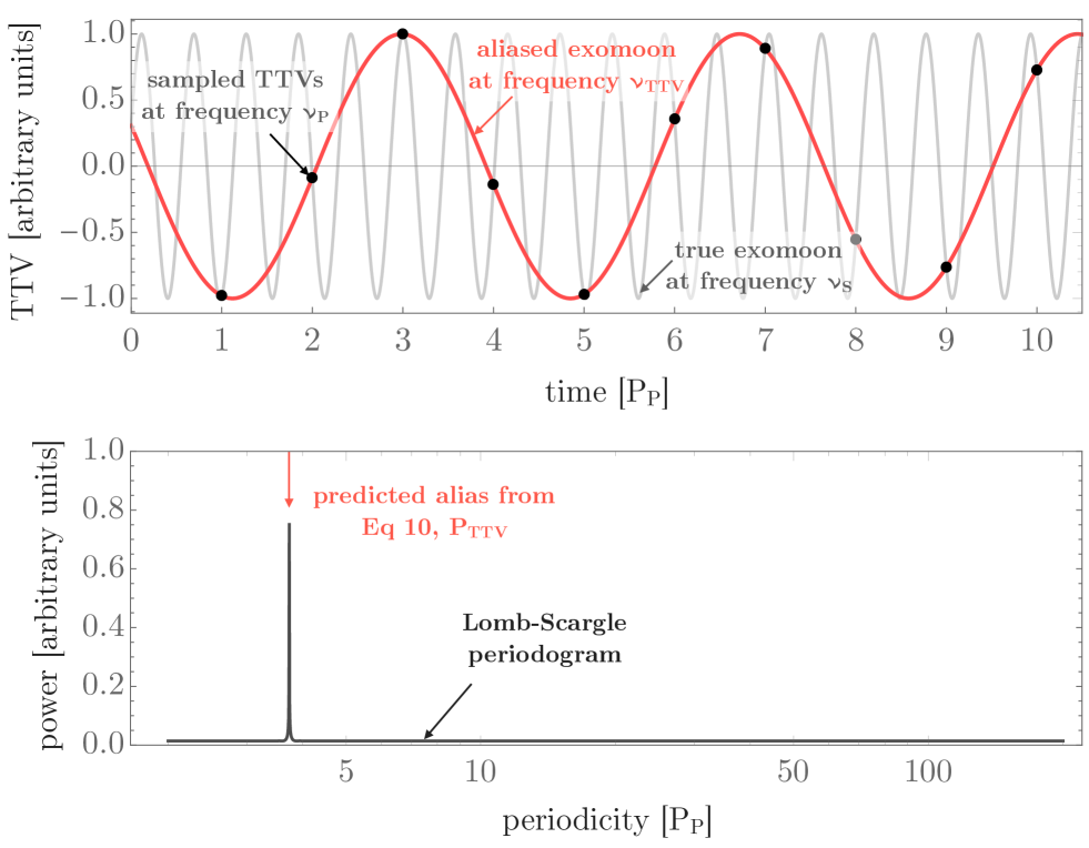
Figure 1: Example of TTV aliasing for a Hill radius exomoon. The moon’s TTV signal (shown in gray) has frequency above the Nyquist rate (this is always true for moons) and thus is perfectly fit by the longer period alias shown in red. The periodogram computed below shows the same effect in the frequency domain.

2.3 Going from observed period to exomoon period

If one observes a TTV signal with a periodicity of $P_{\mathrm{TTV}}$, one now needs to invert Equation (10) back to the true period, $P_{S}$. We find that any $P_{S}$ which satisfies the below expression will be an exact solution to Equation (10):

$$P_{S} =\Big{(}\frac{1}{P_{\mathrm{TTV}}}+n\frac{1}{P_{P}}\Big{)}^{-1},$$ (11)

where $n$ is a positive real integer. If we require that $f<1$ (the satellite is inside the Hill sphere), then we can impose

$$n>\frac{\sqrt{3}}{f^{3/2}}-\frac{P_{P}}{P_{\mathrm{TTV}}}.$$ (12)

For $f<1$ and $P_{\mathrm{TTV}}>2P_{P}$ (the Nyquist periodicity), this always excludes $n=1$ but leaves anything greater than or equal to 2 as a possibility.

A maximum limit on $n$ could be proposed if one adopts some lower limit for $P_{S}$. Io is perhaps the most extreme example of a large moon in close proximity to its planet, residing within at 0.8% of Jupiter’s Hill radius. If we take $f=0.01$ as a fiducial lower limit, then we find that one can fit 1731 unique solutions for $P_{S}$ in-between this limit and the Hill radius. This highlights how challenging and multimodal the exomoon parameter space truly is.

2.4 Probability distribution of TTV periods due to aliased moons

We have now established that i) exomoons always induce undersampled TTVs which manifest as an aliased TTV, and ii) inverting an aliased periodicity back to the true exomoon period is highly multimodal. The last task we address here considers what the probability distribution of these aliased TTV periods are expected to be.

In order to address this, we first need to choose a probability distribution for the exomoon periods. It is convenient to work in units of planetary period for the TTV periods and frequencies, since then the distribution of the $P_{P}$ does not actually affect our results. However, we do still need to choose some distribution for the moons themselves. To this end, we considered four possible toy models:

• Exomoon periods distributed such that they are uniform in frequency space (i.e. uniform in $1/P_{S}$).

• Log-uniformly distribution for $f$, which is equivalent to a log-uniform distribution for semi-major axis $a_{S}$ (and also $P_{S}$).

• Uniformly distribution for $f$, which is equivalent to a log-uniform distribution for semi-major axis $a_{S}$ (but not in $P_{S}$).

• A linearly weighted distribution in moon semi-major axis such that $\mathrm{Pr}(a_{S})\propto a_{S}$.

Whilst the first three are broadly designed to be diffuse, uninformative distributions, the last one encodes a selection bias effect that we are more likely to detect wider orbit moons, since the TTV amplitude is itself proportional to $a_{S}$ (Sartoretti & Schneider, 1999).

We assume a minimum allowed $f=0.01$ and a maximum of $f=0.5$ (Domingos et al., 2006) and generated $10^{6}$ samples from these distributions. The resulting distributions for $\log_{10}f$, $f$, $\nu_{\mathrm{TTV}}$ and $\log_{10}P_{\mathrm{TTV}}$, for all four models, are shown in Figure 2.

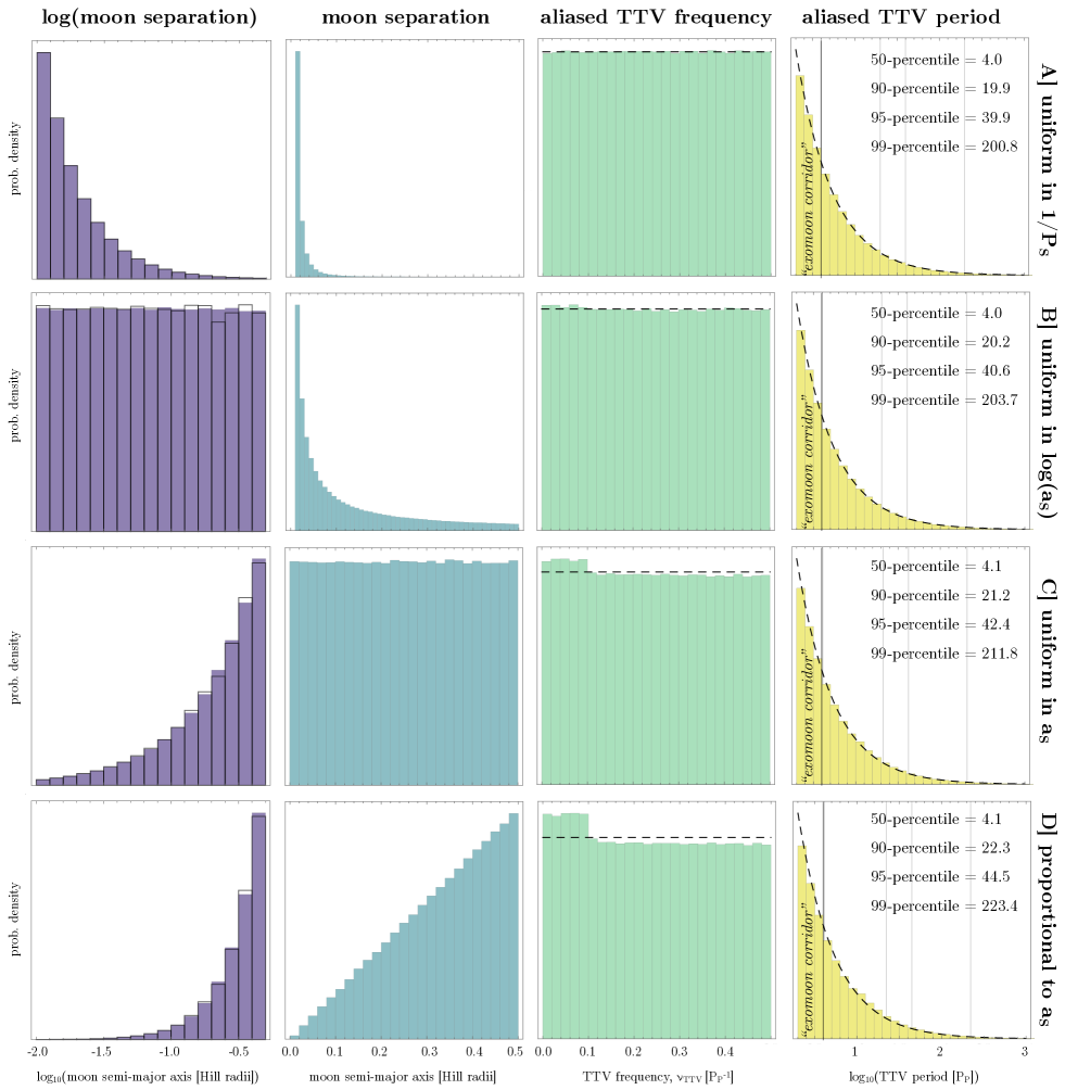
Figure 2: The distribution of four relevant exomoon TTV parameters (the four columns) for four different assumed distributions of exomoons (the four rows). Although the models produce wildly different distributions for the moon separations (left columns), the knock-on effect to the distribution of aliased TTVs is fairly self-similar and thus robust. Vertical grid lines show the median, 90%, 95% and 99% quantiles. Black histograms overlaid on the left column shows the same distribution but applying the filter that the moons must manifest in the labelled “exomoon corridor”. Black dashed lines show an closed-form approximation given by Equation (13).

As evident from the figure, there are very pronounced differences between how the moons are distributed spatially amongst the four models. Yet, despite this, the resulting distribution of aliased TTV frequencies and periodicities are remarkably self consistent. In every experiment, we recover an exponential-like distribution in $\log_{10}P_{\mathrm{TTV}}$ piling up at the Nyquist period. One can see from the quantiles listed on the far right column that the median aliased TTV period is about 4 cycles. In other words, 50% of all exomoons should be expected to produce a TTV aliased period between 2 and 4 cycles, a region we refer to as the “exomoon corridor”.

From Figure 2, we note that the TTV frequency panels exhibit an approximately uniform distribution. If we adopt this as a formal approximation, we can use it to transform into period-space and express a closed-form expression for the period distribution:

$$\mathrm{Pr}(P)\,\mathrm{d}P=\begin{cases}2P^{-2}\,\mathrm{d}P&\text{if }P>2,\\ 0&\text{otherwise }.\end{cases}$$ (13)

This distribution is overplotted in the right-hand panels of Figure 2, where one can see that it provides good agreement to the numerical experiments. The cumulative distribution function of Equation (13) can be trivially shown to yield a median of 4 - thus recovering the observation that 50% of the samples produce a period in the range of 2 to 4 cycles.

2.5 The exomoon corridor as a detection strategy

Given that half of all moons manifest in the corridor, broadly irrespective of their true underlying distribution, this means that any TTV signal in this region could be potentially rapidly identified as an exomoon candidate. If this strategy were implemented, it is natural to ask whether the recovered moons would be in any way biased towards a certain region of parameter space.

To investigate this, we took our four fake moon populations, and filtered on only those samples which ended up in the corridor when considering $P_{\mathrm{TTV}}$. This sub-sample, which represents about the half the population, was then compared to the original injected population to see if any systematic changes had occurred. This is visualized in Figure 2 in the left column, where the colored histograms show the original, injected population and the black outline histograms show the filtered subset. As evident from the figure, the distributions are nearly identical and thus selecting exomoons that live in the corridor will not noticeably bias the recovery of the true population.

Although we have shown that half of all moons will appear in the corridor, this would not be of much practical value if false-positives also preferentially pile-up in this region. As discussed in the introduction of this paper, the most common source of large TTVs is planet-planet interactions and thus it is natural to ask what their $P_{\mathrm{TTV}}$ distribution looks like. One can analytically predict $P_{\mathrm{TTV}}$ for planet-planet interactions, which are typically dominated by the so-called “super-period” of circulating line of conjunctions (Lithwick et al., 2012) and to a lesser degree the “chopping” effect caused by the conjunctions themselves (Nesvorný et al., 2014; Deck & Agol, 2015). However, this calculation is highly sensitive to precise period ratios between planets, which cannot be assumed to be drawn from independent distributions due to the mutual interactions themselves.

Instead, we took the largest catalog of confirmed TTV planets available in the literature from Hadden & Lithwick (2017). Specifically, their Table 2 lists 90 adjacent planet pairs with mutual interactions, from which we calculate the dominant super-period as $P_{\mathrm{TTV}}$ for 180 planets. A histogram of these periods is shown in Figure 3, where one can clearly see a quite distinct distribution from those shown earlier in Figure 2.

Only two out of 180 TTV planets exhibit a TTV super-period in the exomoon corridor i.e ${\simeq}1$%. Given that 50% of moons manifest in the corridor, it might be tempting to assign a ${\sim}$50:1 odds ratio that any signal in this region is moon-like. However, such a simple analysis ignores the observational bias that planet-planet interactions are generally much larger than that due to moons, sometimes of order of many days (Nesvorný et al., 2013), and thus would be overrepresented versus this naive fraction. An accurate false-positive rate would require knowledge of the mass distribution of both interacting planets and exomoons, which for the latter we certainly do not have. Further, there are expected to be other sources of false-positives besides planet-planet interactions, such as spurious TTVs induced by stellar activity (Ioannidis et al., 2016), and transit-phase sampling effects (Kipping & Bakos, 2011; Szabó et al., 2013).

Nevertheless, it is encouraging that planet-planet interactions are expected to rarely produce TTVs in the exomoon corridor. Signals in the region are thus immediately interesting for exomoon follow-up analysis, such as detailed photodynamical modeling (Kipping, 2011). Since such an analysis is computationally expensive (only $\sim 60$ out of the several thousand Kepler candidates have been analyzed thus far; Kipping et al. 2015), the exomoon corridor provides a useful means of rapidly prioritizing interesting candidates for subsequent investigation.

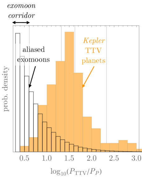
Figure 3: Comparison of the TTV periods for Kepler planet-planet pairs (orange) exhibiting gravitational interactions (Hadden & Lithwick, 2017), versus the predicted distribution of TTV periods caused by aliased exomoons (black). Only ${\simeq}1$% of TTV planets manifest in the “exomoon corridor” of 2-4 cycles.

2.6 Application to Kepler-1625b

As a demonstration of the described technique on an exomoon candidate, we here apply the outlined method to Kepler-1625b i. However, using the 4 available transit times reported in (Teachey & Kipping, 2018), a naive periodogram analysis is problematic. This is because the problem is underdetermined with 5 unknown parameters; 2 linear ephemeris parameters ($P$ and $\tau$) + 3 sinusoid parameters ($A_{\mathrm{TTV}}$, $P_{\mathrm{TTV}}$ and $\phi_{\mathrm{TTV}}$).

A common approach would be to fit a linear ephemeris first, then compute the four residuals to that fit - which defines TTVs. At this point, the problem might seem now overdetermined, since we’d next model the 4 TTVs with a 3-parameter sinusoid. However, this approach is formally wrong since inference of the sinusoid terms would be strictly conditional upon the previously adopted ephemeris. Critically, that ephemeris has uncertainty, it is not known to infinite precision - especially with just 4 available transits. The inter-parameter degeneracies, described by the mutual covariances, mean that this simple approach will not in general yield accurate solutions.

Progress can be made in underdetermined problems through regularization, or in Bayesian parlance, the use of priors. As an example, in machine learning, Lasso regularization is a common strategy to further constrain a problem by appending a new term to the merit function that penalizes large parameter values (Tibshirani, 1995). Priors have a similar effect to regularization, since they add too extra constraints/information into the inference and in many ways can be thought of as an equivalent approach.

To gain some insight into the appropriate regularization here, we first attempted a naive periodogram despite the overdetermined nature (see Figure 4A). Using a log-uniform grid of candidate TTV periods, we fit the now four-parameter model (since $P_{\mathrm{TTV}}$) at each period - yielding in almost every case a perfect fit in a $\chi^{2}$-sense. The only exception to this was at $P_{\mathrm{TTV}}=3$ cycles, which curiously was the only period unable to obtain a perfect fit, with $\chi^{2}=4.75$ (red line in Figure 4B). On the face of it, this periodogram teaches us very little - every period is as good as any other (with one exception). However, if we plot the amplitude of the maximum likelihood sinusoids at each period (see Figure 4A purple line), one sees extremely large amplitudes often being invoked to explain the data. For example, at $P_{\mathrm{TTV}}=2.65$ cycles, the amplitude is nearly 7 days (blue line in Figure 4B and C). Given that the RMS of the four data points is 16 minutes, it seems highly improbable that four randomly drawn points from a 7 day amplitude sinusoid would be so small. Much like Lasso regularization then, we seek to instruct our inference to prefer low amplitude TTVs over high amplitude ones. This can be formally encoded by adding a log-uniform prior to the amplitude of the form $\mathrm{Pr}(A)\sim 1/A_{\mathrm{TTV}}$. We can then add the logarithm of this prior onto the log-likelihood from a simple least squares normal) likelihood function to express a log-posterior probability (unnormalized) for each period grid point. A similar approach has been used for Bayesian radial velocity periodograms (e.g. see Gregory 2007). The resulting periodogram is shown in Figure 4 in black.

The maximum a-posteriori peak is broad, which is not surprising given the poor constraints, but centers on 4.4 cycles. In the context of this paper, this occurs very close to the median period expected from an exomoon. We also note that the existence of TTVs is quite secure at $\Delta\chi^{2}=17.5$; an issue which should not be conflated with the distinct issue of parameter determination. These two points thus show that Kepler-1625b is indeed consistent with the exomoon hypothesis claimed by Teachey & Kipping (2018), using just the transit times alone. To share this maximum a-posteriori best model, we report $A_{\mathrm{TTV}}=17.08$ mins, $P_{\mathrm{TTV}}=4.405$ cycles, $\phi_{\mathrm{TTV}}=1.5478$ rads, $P=287.37221$ days and $\tau=2456043.95957$ BJD_UTC, where we define the median Kepler epoch as the reference ($0^{\mathrm{th}}$) epoch.

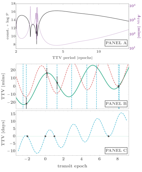
Figure 4: Panel A: Periodogram of the TTVs, with a broad peak occurring at 4.4 cycles (corresponding to $\Delta\chi^{2}=17.7$) - approximately the median TTV period that would be expected from an exomoon. Panel B: Observed transit times of Kepler-1625b from Teachey & Kipping (2018) after subtracting the maximum a-posteriori ephemeris, to yield TTVs. The maximum a-posteriori sinusoid is shown in green with a period of 4.4 cycles. The red line shows the one “bad” period for which a perfect fit could not be obtained. Panel C: A zoom-out of the TTVs showing an example of a perfect fit with a ridiculous amplitude (blue line, which is also present in Panel B). Such fits are strongly disfavoured in our final periodogram through the use of regularization.

3 Discussion

We have shown that TTVs due exomoons will always manifest as longer period aliases in the frequency analysis of such observations. It is possible to analytically express the exact relationship between the exomoon period and the aliased frequency, as given by Equation (10) in this work. Converting these aliased periods back to unique exomoon periods appears intractable with TTVs alone, due to the many hundreds of harmonic solutions which can fit the data. Thus, unique solutions to exomoon data will surely depend on auxiliary information such as transits (Brown et al., 2001; Szabó et al., 2006; Simon et al., 2007; Kipping, 2011) or TDVs (Kipping, 2009a, b; Awiphan et al., 2013).

However, we note that injecting a variety of radically different distributions for the exomoon population into our formula leads to nearly identical resulting distributions for the aliased TTV period (given by Equation 13). Specifically, exomoons produce aliased TTVs that preferentially peak close to the Nyquist periodicity of 2 cycles. Indeed, we estimate that 50% of all exomoons will manifest in a narrow TTV period corridor of 2 to 4 cycles, broadly independent of the assumed exomoon distribution.

This remarkable feature provides an immediate and powerful tool for identifying exomoon candidates. Any TTV signal with a strong peak below 4 cycles is an excellent target for further analysis. Naturally, this information alone does not demonstrate the moon hypothesis and so we caution readers to not abuse this tool. Although planet-planet interactions less frequently manifest at such short periodicities, chopping signals (due to conjunctions) can mimic shorter term variability (Nesvorný et al., 2014; Deck & Agol, 2015), as well as false positives from spots for example (Ioannidis et al., 2016). A detailed investigation of the power spectra of these effects is encouraged for future work. Similarly, planets with very large TTVs would provide non-uniform sampling that may offer access to higher frequencies (Murphy et al., 2013; VanderPlas, 2018), and thus would also be a worthwhile topic of further investigation.

Nevertheless, this work provides a simple and straight forward tool to quickly identifying high priority exomoon candidates suitable for further analysis with tools such as photodynamical modeling.

Data Availablity

The data underlying this article are available via Columbia Academic Commons, at https://doi.org/10.7916/D8795NHS. The datasets were derived from sources in the public domain (Teachey & Kipping, 2018).

References

- Awiphan et al. (2013) Awiphan, S. & Kerins, E., 2013, MNRAS, 432, 2549
- Brown et al. (2001) Brown, T. M., Charbonneau, D., Gilliland, R. L., Noyes, R. W., Burrows, A., 2001, ApJ, 52, 699
- Christiansen et al. (2016) Christiansen, J. L., Clarke, B. D., Burke, C. J., et al., 2016, ApJ, 828, 99
- Dawson & Fabrycky (2010) Dawson, R. I. & Fabrycky, D. C., 2010, ApJ, 722, 937
- Deck & Agol (2015) Deck, K. M. & Agol, E., 2015, ApJ, 821, 96
- Demory et al. (2011) Demory, B. -O., Gillon, M., Deming, D., et al., 2011, A&A, 533, 114
- Domingos et al. (2006) Domingos, R. C., Winter, O. C., Yokoyama, T., 2006, MNRAS, 373, 1227
- Gregory (2007) Gregory P. C., 2007, MNRAS, 374, 1321
- Hadden & Lithwick (2017) Hadden, S. & Lithwick, Y., 2017, ApJ, 154, 5
- Holman et al. (2010) Holman, M. J., Fabrycky, D. C., Ragozzine, D., et al., 2010, Science, 330, 51
- Ioannidis et al. (2016) Ioannidis, P., Huber, K. F., Schmitt, J. H. M. M., 2016, A&A, 585, 72
- Kipping (2009a) Kipping, D. M., 2009a, MNRAS, 392, 181
- Kipping (2009b) Kipping, D. M., 2009b, MNRAS, 396, 1797
- Kipping et al. (2009) Kipping, D. M., Fossey, S. J., Campanella, G., 2009, MNRAS, 400, 398
- Kipping (2011) Kipping, D. M., 2011, MNRAS, 416, 689
- Kipping & Bakos (2011) Kipping, D. M. & Bakos, G. Á., 2011, ApJ, 730, 50
- Kipping et al. (2014) Kipping, D. M., Nesvorný, D., Buchhave, L. A., Hartman, J., Bakos, G. Á., Schmitt, A. R., 2014, ApJ, 784, 28
- Kipping et al. (2015) Kipping, D. M., Schmitt, A. R., Huang, X., Torres, G., Nesvorný, D., Buchhave, L. A., Hartman, J., Bakos, G. Á., 2015, ApJ, 813, 14
- Kipping & Teachey (2020) Kipping, D. M. & Teachey, A., 2020, MNRAS, submitted (arXiv e-prints:2004.04230)
- Lithwick et al. (2012) Lithwick, Y., Xie, J. & Wu, Y., 2012, ApJ, 761, 122
- McClellan et al. (1999) McClellan, J. H., Schafer, R. W., & Yoder, M. A. 1999, DSP First: A Multimedia Approach (Upper Saddle River, NJ: Prentice-Hall)
- Murphy et al. (2013) Murphy, S. J., Shibahashi, H., Kurtz, D. W., 2013, MNRAS, 430, 2986
- Nesvorný et al. (2013) Nesvorný, D., Kipping, D. M., Terrell, D., Hartman, J., Bakos, G. Á., Buchhave, L. A., 2013, ApJ, 777, 3
- Nesvorný et al. (2014) Nesvorný, D., Kipping, D. M., Terrell, D., Feroz, F., 2014, ApJ, 790, 31
- Nesvorný et al. (2014) Nesvorný, D. & Vokrouhlický, D., 2014, ApJ, 790, 58
- Sartoretti & Schneider (1999) Sartoretti, P. & Schneider, J., 1999, A&AS, 14, 550
- Simon et al. (2007) Simon, A., Szatmáry, K., Szabó, Gy. M., 2007, A&A, 470, 727
- Simon et al. (2009) Simon, A., Szabó, Gy. M., Szatmáry, K., 2009, EM&P, 105, 385
- Simon et al. (2015) Simon, A., Szabó, Gy. M., Kiss, L. L., Fortier, A., Benz, W., 2015, PASP, 127, 1084
- Szabó et al. (2006) Szabó, Gy. M., Szatmáry, K., Divéki, Zs., Simon, A., 2006, A&A, 450, 395
- Szabó et al. (2013) Szabó, R., Szabó, Gy. M., Dálya, G., Simon, A. E., Hodosán, G., Kiss, L. L., 2013, A&A, 553, 17
- Teachey et al. (2018) Teachey, A., Kipping, D. M., Schmitt, A. R., 2018, ApJ, 155, 36
- Teachey & Kipping (2018) Teachey, A. & Kipping, D. M., 2018, Science Advances, 4, 178
- Tibshirani (1995) Tibshirani, R., 1995, J. R. Statist. Soc. B., 58, 267
- VanderPlas (2018) VanderPlas, J. T., 2018, ApJS, 236, 16