Identification of AKARI infrared sources by Deep HSC Optical Survey:
Construction of New Band-Merged Catalogue in the NEP-Wide field

Abstract

The north ecliptic pole (NEP) field is a natural deep field location for many satellite observations. It has been targeted many times since it was surveyed by the AKARI space telescope with its unique wavelength coverage from the near- to mid-infrared (mid-IR). Many follow-up observations have been carried out and made this field one of the most frequently observed areas with a variety of facilities, accumulating abundant panchromatic data from X-ray to radio wavelength range. Recently, a deep optical survey with the Hyper Suprime-Cam (HSC) at the Subaru telescope covered the NEP-Wide (NEPW) field, which enabled us to identify faint sources in the near- and mid-IR bands, and to improve the photometric redshift (photo-z) estimation. In this work, we present newly identified AKARI sources by the HSC survey, along with multi-band photometry for 91,861 AKARI sources observed over the NEPW field. We release a new band-merged catalogue combining various photometric data from GALEX UV to the submillimetre (sub-mm) bands (e.g., Herschel/SPIRE, JCMT/SCUBA-2). About $\sim$ 20,000 AKARI sources are newly matched to the HSC data, most of which seem to be faint galaxies in the near- to mid-infrared AKARI bands. This catalogue motivates a variety of current research, and will be increasingly useful as recently launched (eROSITA/ART-XC) and future space missions (such as $JWST$, Euclid, and SPHEREx) plan to take deep observations in the NEP field.

1 Introduction

To answer the questions concerning cosmic star formation history and galaxy evolution, it is critical to have a comprehensive understanding of the infrared (IR) luminous population of galaxies (Casey et al., 2014; Kirkpatrick et al., 2012; Madau & Dickinson, 2014; Sanders et al., 2014). They are presumably star-forming systems containing a large amount of dust, where the critical phase in their activities of star formation (SF) or active galactic nuclei (AGN) take place, hidden behind the obscuring dust (Galliano et al., 2018; Goto et al., 2010; Hickox & Alexander, 2018; Lutz, 2014).

Wide-field cosmological surveys at IR wavelengths are the most efficient way to collect data for various populations of galaxies, especially for dusty star-forming galaxies (dusty SFGs, DSFGs) and obscured AGNs, at different cosmological epochs (Matsuhara et al., 2006; Hwang et al., 2007, 2010; Toba et al., 2015). Statistically significant samples of dusty galaxies based on large-area surveys covering significant cosmological volumes have to be obtained. Also, follow-up surveys should be made to sample spectral energy distributions (SEDs): a comprehensive physical description requires wide wavelength coverage to capture the range of processes involved. Most importantly, a deep optical follow-up survey is necessary because the optical identification is an essential prerequisite to understand nature of the sources (Sutherland & Saunders, 1992; Hwang et al., 2012), e.g., star-galaxy separation or to derive photometric redshift (photo-z).

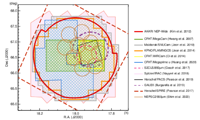
Figure 1: An overall map showing a variety of surveys around the NEP. The red circular area shows the AKARI’s NEP-Wide field (Kim et al., 2012). The green and grey (meshed) areas represent the optical surveys done with the CFHT MegaCam (Hwang et al., 2007) and the Maidanak SNUCam (Jeon et al., 2010), respectively. The yellow square shows a slightly deeper observation with the MegaCam as well as the WIRCam on the NEP-Deep field (Oi et al., 2014). The area surrounded by blue line shows the additional u-band observation by the MegaPrime (Huang et al., 2020). The pink shaded area indicates the recent near-IR survey with Spitzer (Nayyeri et al., 2018). The small black square inside the yellow box shows the area observed by the Herschel/PACS (Pearson et al., 2019). A broken magenta circle overlaid with the black square indicates the area observed by S2CLS (Geach et al., 2017). Nine brown circles around the S2CLS show the areas surveyed by NEPSC2 850 $\mu$m mapping program with SCUBA-2 (Shim et al., 2020). The largest rhombus (brown long-dashed line) shows the Herschel/SPIRE coverage (Pearson et al., 2017).

The north ecliptic pole (NEP; $\alpha=18^{h}00^{m}00^{s}$, $\delta=66^{\circ}33^{\prime}88^{\prime\prime}$) has been a good target for deep, unbiased, and contiguous surveys for extra-galactic objects such as galaxies, galaxy clusters and AGNs because the NEP is a natural deep field location for a wide class of observatory missions (Serjeant et al., 2012). Many astronomical satellites, such as ROSAT (Henry et al., 2006), GALEX (Burgarella et al., 2019), Spitzer Space Telescope (Jarrett et al., 2011; Nayyeri et al., 2018), have accumulated a large number of exposures towards the NEP area because the Earth-orbiting satellites pass over the ecliptic poles and, for the Earth-trailing satellites, these poles are always in the continuous viewing zone. The AKARI (Murakami et al., 2007) also devoted a large amount of observing time (a span of more than a year) to cover a wide area over the NEP using the infrared camera (IRC, Onaka et al., 2007) with excellent visibility thanks to its polar sun-synchronous orbit (Matsuhara et al., 2006).

A noticeable aspect of this NEP field surveyed by AKARI is that the ancillary optical data sets are abundant, supporting the identification of the infrared sources which enabled subsequent analyses properly (Kim et al., 2012). In addition, many other surveys or follow-up observations on the NEP (but on a limited area) have been carried out from X-ray to radio wavelengths to cover the NEP area (Krumpe et al., 2015; Burgarella et al., 2019; Pearson et al., 2019; Geach et al., 2017; White et al., 2010, 2017) since the AKARI obtained valuable data sets (see Figure 1). However, a fraction ($\sim 30\%$ at $N4$) of the IR sources detected by AKARI has been left unidentified by optical data because of the insufficient depths and incomplete areal coverage of the previous optical surveys. The different photometric filter systems used at different surveys also hampered homogeneous analyses based on unbiased sample selection, therefore a deeper and coherent optical survey on this field was necessarily required.

A new deep optical survey consistently covering the entire NEP-Wide (NEPW) field was carried out by the Hyper Suprime-Cam (HSC: Miyazaki et al., 2018) with five photometric filter bands ($g$, $r$, $i$, $z$ and $y$). These HSC data were reduced (Oi et al., 2020) by the recent version of the pipeline (v6.5.3, Bosch et al., 2018), which allowed the depth of the new optical data to reach down to $\sim$ 2 mag deeper (at $g$ and $i$ band) than the previous optical survey with Canada-France-Hawaii Telescope (CFHT, Hwang et al., 2007). In addition, supplemental observation using the CFHT/MegaPrime (Huang et al., 2020) replenished the insufficient coverage of $u^{*}$-band from the previous CFHT surveys, which brings photo-z accuracy improvement along with this new HSC data (Ho et al., 2020). The source matching and band merging process (see Section 2 for the details) have been encouraging various subsequent works such as the recent luminosity function (LF) update (Goto et al., 2019), properties of mid-IR (MIR) galaxies detected at 250$\mu$m (Kim et al, 2019), estimation of number fraction of AGN populations (Chiang et al., 2019), study on high-z population (Barrufet et al., 2020), obscured AGN activity (Wang et al., 2020), merger fraction depending on star formation mode (Kim et al. in prep), AGN activities depending on the environments (Santos et al. in prep), machine learning algorithms to classify/separate IR sources (Poliszczuk et al. in prep; Chen et al. in prep), cluster candidates finding (Huang et al. in prep), and even on the AKARI sources without any HSC counterpart (Toba et al., 2020). The science on the NEP initiated by AKARI is now entering a new era with a momentum driven by Subaru/HSC observations as well as current survey projects, such as homogeneous spectroscopic survey (MMT2020A/B, PI: H. S. Hwang) and the 850 $\mu$m mapping over the entire NEP area using with the Submillimetre Common-User Bollometric Array 2 (SCUBA-2) at the James Clerk Maxwell Telescope (Shim et al., 2020). More extensive imaging observations with HSC are still on going with spectroscopy with Keck/DEIMOS+MOSFIRE as part of the Hawaii Two-O project (H20). Spitzer also finished its ultra deep NIR observations recently as one of the Legacy Surveys (PI: Capak) before it retired early 2020 to carry out precursor survey for Euclid (Laureijs et al., 2011), the James Webb Space Telescope (JWST, Gardner et al., 2006) and the Wide Field InfraRed Survey Telescope (WFIRST: Spergel et al., 2015) over this field. The Spektr-RG was launched in 2019 to the L2 point of the Sun-Earth system (1.5 million km away from us) and eROSITA(Merloni et al., 2012) started mission towards the NEP. Spectro-Photometer for the History of the Universe, Epoch of Reinonization, and Ice Explorer (SPHEREx: Doré et al., 2016, 2018) are also planning to target this field.

The main goal of this work is to identify optical counterparts of the AKARI/NEPW sources with more reliable optical photometry of the HSC images (even for the faint NIR sources), and cross-check with all available supplementary data covering this field to build the panchromatic data. We briefly describe various data supporting AKARI/NEPW data, but mostly focus on explaining how we matched sources and combined all the data together. This paper is organised as follows. Sec. 2 introduces the HSC and AKARI data, and gives the detailed process how we cross-matched the sources between them. In Sec. 3, we present the complementary data sets used to construct the multi bands catalogue. We describe their optical-IR properties (in statistical ways) in Sec. 4. Sec. 5 gives the summary and conclusions. All magnitudes are presented in AB the magnitude system.

2 Identification of the AKARI’s NEP-Wide sources using deep HSC data

2.1 AKARI NEP-Wide survey data

The NEP-Wide (NEPW) survey (Matsuhara et al., 2006; Lee et al., 2009; Kim et al., 2012), as one of the large area survey missions of the AKARI space telescope (Murakami et al., 2007), has provided us with a unique IR data set, sampling the near- to mid-IR wavelength range without large gaps between the filter bands (the circular area surrounded by a thick red line in Figure 1). In this program, they observed the 5.4 deg² circular area centred at the NEP using nine photometric bands covering the range from 2 to 25 $\mu$m continuously. The overall strategy of the survey was explained by Lee et al. (2009). Kim et al. (2012) presented the description of the data reduction, source detection, photometry, and catalogue. They also combined the nine separated catalogues (i.e., for $N2$, $N3$, $N4$ in the NIR, $S7$, $S9W$, $S11$ in the MIR-S, and $L15$, $L18W$, $L24$ in the MIR-L channel) along with the optical identification/photometry. Before combining, they carefully discriminated the spurious objects and false detection, in order to confirm the validity of the IR sources: they tried to identify the optical counterparts using the CFHT (Hwang et al., 2007) and Maidanak (Jeon et al., 2010) data and then cross-checked against the NIR $J$, $K$ band data obtained from the KPNO/FLAMINGOS (Jeon et al., 2014).

The number of sources detected at the nine IRC bands (DETECT_THRESH=3, DETECT_MINAREA=5) by SExtractor (Bertin & Arnouts, 1996) are 87858, 104170, 96159, 15390, 18772, 15680, 13148, 15154, and 4019 (the detection limits are 21 mag in NIR, 19.5 - 19 mags in MIR-S, and 18.6 - 17.8 mags in MIR-L), respectively (Kim et al., 2012). A significant fraction of these sources (17 % of the $N2$, 26 % of the $N3$, and 30 % of $N4$ sources) did not have optical data (mostly because they are not detected in optical surveys). In addition, $\sim$ 4 % of the NIR sources were finally rejected because they are detected at only one NIR band (e.g., $N2$, $N3$, or $N4$) and are strongly suspected to be false objects: they suffered from the ‘multiplexer bleeding trails’ (MUX-bleeding) due to the characteristics of the InSb detector array (Holloway, 1986; Offenberg et al., 2001) so that the source detection near the MUX-bleeding was strongly affected by artificial effects and spurious objects near the abnormally bright pixels. Also, the false detection caused by cosmic ray hits were serious at the $N4$ band mostly because the telescope time to take dithering frames was sometimes assigned to the telescope maneuvering (by the IRC03 observation template). If a certain source were detected at only one NIR band, it could potentially be an artifact or false detection. Therefore, the sources detected at only one NIR band were excluded in the first release of the band-merged NEPW catalogue. In the MIR bands, cosmic ray hits and other artifacts are not numerous, and so the sources detected by only one MIR band were included.

Note that the AKARI NEP-Deep (NEPD) survey data (Wada et al., 2008; Takagi et al., 2012), which is similar to the NEPW survey (with the consistent photometries and the same astrometric accuracy) but different in terms of the coverage (0.7 deg²) and the depth ($\sim$ 0.5 mag deeper), is not included in this work.

We expect that the new optical data obtained by the HSC (Oi et al., 2020) will allow us to identify more IR sources, most of which are faint in the IR as well as the optical bands. Also, we may be able to examine if there are any real NIR sources that have been rejected just because they did not have any counterpart against the other bands (from the optical to MIR). We, therefore, repeated the merging of nine AKARI bands without any exclusion process, in order to attempt to recover possibly real AKARI sources not included in the study of Kim et al. (2012). The sources detected at least one AKARI band can be included in the new AKARI 9 bands merged catalogue. Spurious objects or artifacts can be excluded later if we find any, during further analyses.

When we carried out this procedure, we began with the matching between $N2$ and $N3$ band first. After that, we used these results against the $N4$ band using $N3$ coordinates. In the case without $N3$ coordinates (i.e., a source detected at $N2$ but not detected at $N3$), we took $N2$ coordinates for the matching against $N4$. This process went through down to the $L18W$ or $L24$. In the resulting catalogue, we kept the coordinates from the shortest and the longest bands in this matching process. Therefore, if a certain source was detected at neither $N2$ nor $L24$ but at the other bands, then the coordinates information for the shortest band is from $N3$ and the longest from $L18W$. There is no systematic offset among the astrometry from different AKARI bands (all of them are fixed at the same focal plane). We eventually registered 130,150 IR sources in the new NEPW catalogue, which were detected at least one of the AKARI bands from $N2$ to $L24$.

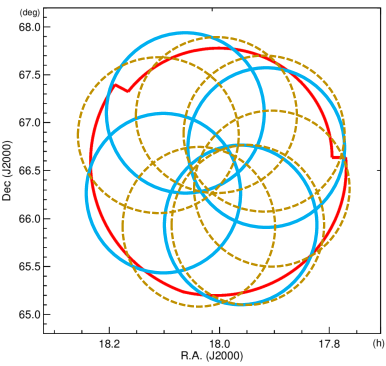
Figure 2: The map showing the HSC coverage over the NEPW survey area (a red circular area; Kim et al. 2012). The areas marked by yellow dashed circles show the region observed by the HSC $r$-band, while the four blue solid circles indicate the region observed by the $g$, $i$, $z$, and $y$-band (Oi et al. 2020).

2.2 Deep Optical Survey with HSC over the NEP

A deep optical survey covering the whole NEP field with the HSC was proposed (Goto et al., 2017) in order to detect all the IR sources observed by AKARI. Two optical datasets, one obtained with the CFHT (the central green square in Figure 1; Hwang et al., 2007) and one with Maidanak telescope (the grey area in Figure 1; Jeon et al., 2010) have been supporting the AKARI IR data. However, the depths (5$\sigma$) of these optical surveys (25.4 and 23.1 AB mag at $r^{\prime}$ and $R$ band, respectively) were insufficient to identify all the AKARI IR sources. A slightly deeper observation by MegaCam, (Oi et al., 2014) on a smaller field was also carried out, but the areal coverage (0.67 deg²) was only for the NEPD field (a yellow box in Figure 1).

Goto et al. (2017) intended to use the large field of view (FoV; 1.5 deg in diameter, see Figure 2) of the HSC so that the entire NEPW field of AKARI was able to be covered by taking only 4 FoVs (for the $g$, $i$, $z$, and $y$ bands; the blue circles in Figure 2). Ten FoVs, in total, were allocated in six nights (Goto et al., 2017; Oi et al., 2020) including $r$ band to take the whole NEPW field using those five HSC filter bands. The $r$ band imaging was taken earlier during the first observation in 2014, where the observations suffered from air disturbance (including the dome shutter opening error), which made the seeing at $r$ band worse (1^′′.25) than those of the other four (0.7 – 0.8^′′ ) obtained later in the second observations (Aug. 2015) (Oi et al., 2020).

The data reduction was carried out with the official HSC pipeline, hscPipe 6.5.3 (Bosch et al., 2018). Apart from the fundamental pre-processing procedures (e.g., bias, dark, flat, fringe, etc.), the performance in the sky subtraction and artifact rejection was enhanced in this recent version. In particular, the peak culling procedure was included to cull the spurious or unreliable detections, which improved the source detection results in the pipeline process. Owing to the bad seeing ($\sim 1^{\prime\prime}.25$) in the $r$ band, the source detection was carried out on the $gizy$ band stacked image. However the photometry was forced to be performed at all five bands. All these procedures with recent pipeline (e.g., updated flag information of the hscPipe 6.5.3 (Bosch et al., 2018)) eventually helped resolve the issues that have been reported for a few years regarding false detections (e.g., damaged sources near the boundary or along the image edge of each frame, and effects from the saturation of bright stars, etc.). The 5$\sigma$ detection limits are 28.6, 27.3, 26.7, 26.0, and 25.6 mag at $g$, $r$, $i$, $z$, and $y$, respectively. The limiting magnitudes of the $g$, $r$, $i$, and $z$ band of the previous CFHT data were 26.1, 25.6, 24.8, and 24.0 mag, respectively. We, therefore, obtained 1.7 – 2.5 mags deeper optical data at the corresponding filter bands (even though the effective wavelengths of the filters are slightly different; see Table 1). Finally, we catalogued 3.25 million sources observed by the optical survey with the HSC along with a large number of parameters appended from the HSC data pipeline.

The magnigude at each band was given in terms of the Cmodel photometry, which performs well for galaxies and asymptotically approaches PSF photometry for compact sources. The colours estimated with Cmodel flux are robust against seeing conditions (Huang et al., 2018). As we mentioned in the previous paragraph, seeing conditions for $r$-band are different from the other four bands, therefore by taking Cmodel flux to calculate colours, these different seeing condition effects can be compensated.

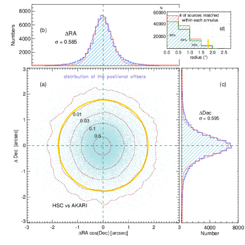
Figure 3: The positional offset distribution of the matched sources between the HSC and AKARI data. On the bottom left panel (a), the dotted contours with numbers represent the density levels normalised by the central peak density. The yellow circle is the matching radius determined based on the 3-sigma ($\sigma$) of the Gaussian, fitted to the histograms (magenta curves), on the top left (b) and bottom right (c) panels, shown in terms of 0.2^′′ bin. On a top right box (d), bars show how many sources were matched within the 0.5^′′ annuli (the green bars indicate the number of clean sources, the red bars above green ones show the increments by the flagged sources. See sec. 2.3 for the details).

2.3 Matching of the AKARI Infrared sources against the HSC optical data

After AKARI band merging (Section 2.1), we performed source matching between the AKARI and HSC data. To identify the counterparts from each other by positional matching, a reasonable search radius was assigned. Figure 3 summarises how we decided the radius for the source matching between the AKARI and the HSC data.

In Figure 3, the bottom left panel (Figure 3a) shows the distribution of the positional offsets of the matched sources on the $\Delta$RA versus $\Delta$Dec plane (before the decision of the radius, we used 3^′′ as a tentative criterion). The contours in the reddish dotted lines with numbers represent the number density of the green dots normalised by the peak value at the center. A yellow circle indicates the 3-sigma ($\sigma$) radius determined based on the Gaussian (magenta curves) fitted to the histograms on the top left (Figure 3b) and the bottom right (Figure 3c) panels. Here, 3-$\sigma$ radius corresponds to 1^′′.78, where the source density in the $\Delta$RA$cos$(dec) vs $\Delta$Dec plane approaches down to the 1 $\%$ level compared to the density peak.

Within this matching radius, we have 111,535 AKARI sources matched against the HSC optical data, which were finally divided into two groups: the clean (91,861) vs. flagged (19,674) sources based on the HSC flag information such as base$\_$PixelFlags$\_$flag$\_$bad (to discriminate bad pixels in the source footprint), base$\_$PixelFlags$\_$flag$\_$edge (to indicate a source is in the masked edge region or has no data), base$\_$PixelFlags$\_$flag$\_$saturatedCenter (to notice that saturated pixels are in the center of a source). These parameters helped us when we discriminated unreliable results with the saturated sources or ones lying at the image edge/border. In this work, we construct a band-merged catalogue only for the “clean" sources, excluding the flagged ones because the derivation of photo-z or physical modeling by SED-fitting requires accurate photometry.

The remaining 23,620 sources did not match to any HSC data (i.e., none-HSC, hereafter), some of which seem to be obscured objects in the optical bands, residing in the high-z ($>1$) universe (Toba et al., 2020).

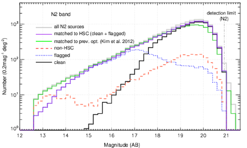
Figure 4: The number distribution of $N2$ sources as a function of magnitude (0.2 mag^-1 deg^-2). All $N2$ sources are divided into three sub-categories according to the matching results against the HSC data: clean (sold black), flagged (dotted blue), and none HSC (dashed red). The violet line shows the optically matched sources (i.e., the sum of the clean and flagged sources). The grey line shows all the $N2$ sources (i.e., the sum of the clean, flagged, and none HSC sources). Green line represents the $N2$ sources matched to the previous optical data from the CFHT or Maidanak (Kim et al., 2012).

The histogram on the top right panel (in Figure 3d) shows the distribution of the matched sources as a function of radius interval. The green (red) bars show the number of the clean (flagged) sources matched in each radius bin with the 0.5^′′ width. A yellow mark indicates the matching radius (1.78^′′, therefore all the sources in the 1.5–2.0 bin are matched within this radius). The green histogram shows that half of the clean sources (48%, 43,789) are matched within 0.5^′′ positional offsets and 34% (31,215) are matched with the offsets between 0.5 – 1.0^′′. Therefore, within a 1^′′ radius, we have 82$\%$ (75,000) sources in total, matched between the AKARI and the HSC data without flagging. Within a 1.5^′′ radius, we have 95$\%$ of the sources (87,645) matched.

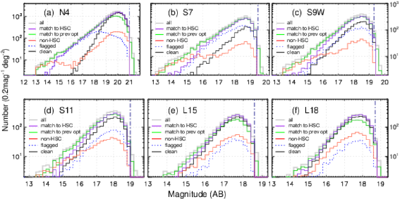
Figure 5: The number distribution of the sources as a function of magnitude, plotted in the same fashion as Figu. 4, but for the sources in the other AKARI bands. Distribution for three different sub-categories are given in the same colour as shown in Figure 4. Vertical dot-dashed line in each panel represents the detection limit in Table 1.

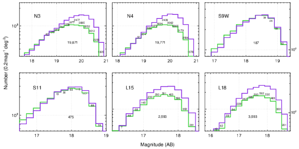
Figure 6: Selected narrow ranges from the Figure 5 near the peak of the histograms (to show the green and violet lines), which give the comparison between the sources matched to the HSC data (violet) and to the previous optical data obtained with the CFHT and Maidanak (green). The small numbers written on the green histogram represent the difference between the violet and green histogram in each magnitude bin, i.e., newly matched to the HSC data. The sum of the small numbers are presented in the middle of each panel. In this range, the violet histogram lower than green one (in the bright side) seems mostly due to the flagged sources (blue dotted line in Figure 5) excluded in this work.

We describe the details of the matching results in Figure 4, which compares the distribution of sub-categories of the sources divided into three (clean, flagged, and none-HSC) as a function of $N2$ magnitude. A grey-coloured histogram indicates all the $N2$ sources which corresponds to the sum of three (clean $+$ flagged $+$ none-HSC) groups. A violet histogram shows the $N2$ sources that have HSC counterpart (clean $+$ flagged). On the other hand, the green line shows the distribution of the $N2$ sources matched to the previous optical data (CFHT and/or Maidanak).

In the bright magnitude range (up to 14.8 mag), there are no clean sources: all the sources are ‘flagged (blue dotted)’ or ‘none HSC (red dashed)’, which means that most of the bright $N2$ sources are accompanied by one of three HSC flags used to filter out the problematic sources or do not have HSC counterpart. This indicates that their HSC counterparts were affected by saturated/bad pixels, masked/edge region, or do not have valid HSC parameters, otherwise they did not match to any HSC sources. Between 13.5 and 17.5 mag, the flagged sources prevail. The clean sources (black line) begin to appear around 15 and go above the flagged sources at 17.5, and this predominance continues to the faint end. The N2 source counts decrease rapidly before the detection limit due to source confusion (Kim et al., 2012). We did not include the sources fainter than the detection limit (i.e., a small number of objects fainter than the vertical dot-dashed line as shown in Figure 4). Some of the none-HSC sources have optical counterparts in the previous CFHT/Maidanak data (in the brightest range) because they are located in the region where the $gizy$ bands (which were used for the source detection) did not cover but the CFHT/Maidanak surveys provided normal photometric measurements (see the small bump in the red dashed histogram below the green one around 13 – 14 mag.). These sources are beyond the concern of this work and the AKARI sources classified into flagged and/or none HSC group might be discussed later (in separate works).

The same description for the other AKARI bands are summarised in Figure 5. The overall trends in the NIR bands is similar to $N2$: the red histogram on the top left panel (Figure 5a for the $N4$ band) shows a smaller bump around 14 mag and the other peak around 20 mag. The smaller bump is ascribed to the unobserved area, otherwise they are probably the brightest stars (almost all the NIR sources brighter than 15 mag seem to be stars; (Kim et al., 2012)), but rejected by the pipeline or classified as flagged. Figure 5a also shows there is no clean source brighter than 16 mag. This trend in the bright end weakens/disappears as we move to the mid-IR bands. It seems that the saturation levels of the HSC bands (17 - 18 mag, Aihara et al., 2018) correspond to the valley between two red bumps in the NIR bands, where the clean sources begin to appear. The smaller red bump fades out in the longer wavelength (MIR) bands: it becomes weak in the $S7$ (Figure 5b), appears weaker in the $S9W$ (Figure 5c), and completely disappears in the MIR-L bands, implying the Rayleigh-Jeans tail of the stars fades out. In the NIR bands, the number of clean sources (black solid line) are higher than those of flagged sources (blue dotted) near the broad peak. In the $S9W$ bands, these two classes become comparable, while the none-HSC sources are much lower. In the $S9W$ and $S11$ bands, the fraction of the flagged sources (blue dotted) are between the black and the red lines. In the MIR-L bands, the blue dotted line becomes lower than none HSC sources (red line).

While some of the bright IR sources are not fully available in this work consequentially because they are unobserved/rejected or eventually classified as flagged sources, on the other hand, there are many more fainter sources newly matched to the deeper HSC data as shown in Figure 6 (for example, 19,771 at $N4$, and 2,593 at $L15$, respectively). Only small ranges were presented in the figure: note the range where the violet histogram is higher than the green one. The number in each magnitude bin indicate the sources newly matched to the HSC data.

However, the bigger red bumps (in Figure 5) near the faint ends indicate our HSC survey was still not deep enough to identify all the faint IR sources, which left some of the AKARI sources unmatched against the HSC data. On the AKARI colour-colour diagrams (in sec. 4), these faint IR sources are located in the same area as the other (optically identified) sources, which implies that they have the similar IR properties. They are probably infrared luminous SFGs, but appear to have dropped out in the HSC bands. Seemingly, they might be a certain kind of highly obscured dusty systems in high-z. A detailed discussion based on the selected sample is presented in Toba et al. (2020).

Table 1: Summary of the multiwavelength data sets: the detection limits

Data	Band	Effective wavelength	(5$\sigma$) detection limit
		($\mu$m)	AB / $\mu$Jy
	$N2$	2.3	20.9 / 15.4
	$N3$	3.2	21.1 / 13.3
AKARI/IRC	$N4$	4.1	21.1 / 13.6
NEP-Wide Survey	$S7$	7	19.5 / 58.6
5.4 deg2	$S9W$	9	19.3 / 67.3
(Kim et al., 2012)	$S11$	11	19.0 / 93.8
	$L15$	15	18.6 / 133
	$L18W$	18	18.7 / 120
	$L24$	24	17.8 / 274
	$g$	0.47	28.6 / 0.01
Subaru/HSC	$r$	0.61	27.3 / 0.04
5.4 deg2	$i$	0.76	26.7 / 0.08
(Oi et al., 2020)	$z$	0.89	26.0 / 0.14
	$y$	0.99	25.6 / 0.21
CFHT/MegaPrime	$u$	0.36	25.4 / 0.25
3.6deg2(Huang et al., 2020)
	$u^{*}$	0.39	26.0 / 0.16
CFHT/MegaCama	$g$	0.48	26.1 / 0.13
2 deg2 (Hwang et al., 2007)	$r$	0.62	25.6 / 0.21
0.7 deg2 (Oi et al., 2014)	$i$	0.75	24.8 / 0.39
	$z$	0.88	24.0 / 0.91
Maidanak/SNUCam	$B$	0.44	23.4 / 1.58
4 deg2 (Jeon et al., 2010)	$R$	0.61	23.1 / 2.09
	$I$	0.85	22.3 / 4.36
KPNO/FLAMINGOS	$J$	1.2	21.6 / 8.32
5.1 deg2 (Jeon et al., 2014)	$H$	1.6	21.3 / 10.96
CFHT/WIRCam	$Y$	1.02	23.4 / 1.58
0.7 deg2 (Oi et al., 2014)	$J$	1.25	23.0 / 2.29
	$K_{S}$	2.14	22.7 / 3.02
Spitzer/IRAC	IRAC1	3.6	21.8 / 6.45
7 deg2 (Nayyeri et al., 2018)	IRAC2	4.5	22.4 / 3.95
0.4 deg2 (Jarrett et al., 2011)	IRAC3	5.8	20.3 / 27.0
	IRAC4	8	19.8 / 45.0
	W1	3.4	18.1 / 18
WISE	W2	4.6	17.2 / 23
(Jarrett et al., 2011)	W3	12	18.4 / 139
	W4	22	16.1 / 800
Herschel/PACSb	Green	100	14.7 / 4.6 mJy
0.44 deg2 (Pearson et al., 2019)	Red	160	14.1 / 8.7 mJy
Herschel/SPIREc	PSW	250	14 / 9.0 mJy
9 deg2 (Pearson et al., 2017)	PMW	350	14.2 / 7.5 mJy
	PLW	500	13.8 / 10.8 mJy
SCUBA-2/NEPSC2d	850	850	1.0 - 2.3 mJy
2 deg2 (Shim et al., 2020)

(a) The detection limits refer to the 4$\sigma$ flux over a circular area with a diameter of 1^′′. (b) The detection limits refer to 3$\sigma$ instrumental noise sensitivities. (c) The detection limits refer to the Open Time 2 (OT2) sensitivity. (d) The detection limits refer to the 1-$\sigma$ rms noise (or 4.7-11 mJy at 80% completeness).

3 Complementary Data Sets

After the identification of $AKARI$ IR sources with the HSC optical data, we used all available photometric catalogue/data over the NEPW field to construct multi-band catalogue. In this section, we briefly describe the data sets used in this work. Just as Figure 1 showed the coverages of various surveys, Table 1 and Figure 7 summarise the photometric bands and depths of the surveys. Figure 7a also shows why source detection changes in different instrument/filter systems.

3.1 Ancillary Optical Data: CFHT and Maidanak

It is not easy to take the entire 5.4 deg² area in a uniform manner unless we have a large-FoV instrument with an appropriate filter system covering a good enough wavelength range. This was what made our previous optical surveys divided into two different data sets 10 years ago: one obtained with the MegaCam ($u^{*}$, $g$, $r$, $i$, $z$) on the central 2 deg² area, and the other with SNUCAM $B$, $R$, and $I$ (Im et al., 2010) of the Maidanak observatory over the remaining part of the NEPW field. The detailed description of these two surveys can be found from Hwang et al. (2007) and Jeon et al. (2010), respectively. However, the western half of the central CFHT field was not observed by $u^{*}$ band. Also, due to the different filter systems and depths between these two optical surveys, homogeneous analysis with optical counterparts over the whole field was practically impossible. Another optical survey was carried out later (Oi et al., 2014) on the NEPD field ($\sim$0.7 deg²) and finally provided MegaCam $u^{*}$ data for the western half area as well as the supplementary WIRcam data ($Y,J,K_{s}$). In addition, the CFHT MegaPrime $u$-band observation was performed over a 3.6 deg² area on the eastern side of the NEPW field (Huang et al., 2020) to replenish the insufficient (central 2 deg² only; see Figure 1) coverage of the MegaCam $u^{*}$-band. Because how to calibrate photo-z is a significant issue under the circumstances that a huge number of sources remain without redshift information, availability of u-band data is crucial to check the UV extinction properties and to improve photo-z accuracy (Ho et al., 2020). We combined all these supplementary optical data: a small systematic shift of WCS ($<1^{\prime\prime}$) in each optical data with respect to the HSC were corrected first, and the matching radii for each data were decided based on the mean positional differences (see Figure 8). The number of sources matched to the HSC data are summarised in Table 2.

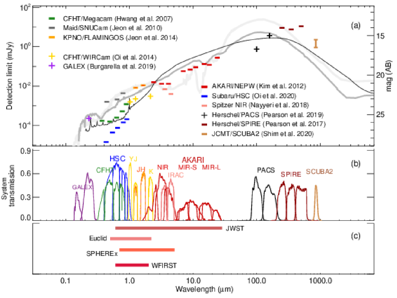
Figure 7: (Top) The depths of various surveys with different instruments/filter systems over the NEP, in terms of the 5-sigma limiting magnitude. The cross symbols (+) imply that the survey was dedicated only to the NEPD field. Typical templates (Polletta et al., 2007) are given to show how a local ULIRG (e.g., Arp220-type at z=0.3, faintest thick line), a type-1 Seyfert (at z=0.6, dark grey), or a dusty torus model (at z=1.0, black thin line) looks in this plot. All of them are normalised at $N2$ detection limit. (Middle) The system transmission/filter shapes are presented. (Bottom) The comparison of the spectral range in the IR to be covered by the future space missions is presented, as shown by the horizontal bars.

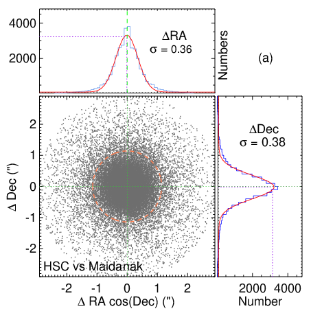
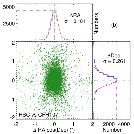
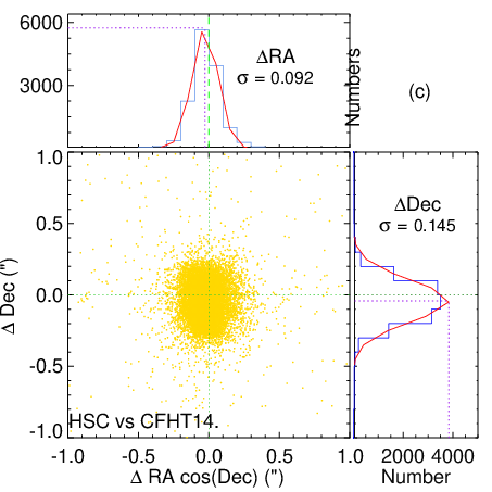
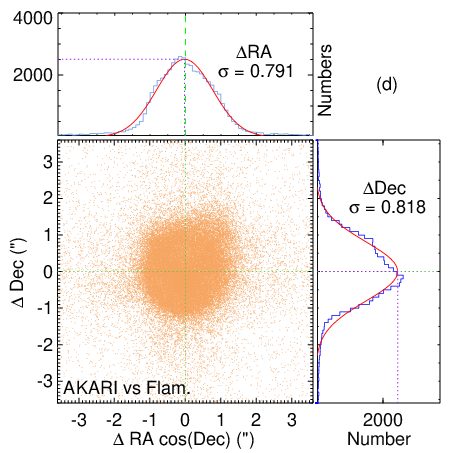
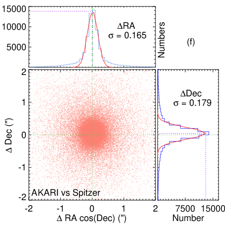
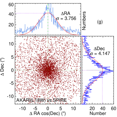
Figure 8: Some examples of the astrometry-offset distributions of the sources matched between the clean (HSC-AKARI) and the other supplementary data. The matching circles (or ellipses) were decided based on the representative value of the offset (width of the offset histogram), 3-$\sigma$ derived from the Gaussian fit to the histogram of $\Delta$RA and $\Delta$Dec. Most of them appear to be circular shape except for the matching against the CFHT data. (a) HSC vs Maidanak (b) HSC vs CFHT (2007) (c) HSC vs CFHT (2014) (d) AKARI vs FLAMINGOS (e) AKARI vs WISE (f) AKARI vs Spitzer (g) AKARI (MIR-L) vs SPIRE.

Table 2: Summary of the Matching against the Supplementary Data

Main Data	Supplementary Data	3-$\sigma$ Radius	PSF Size	Number of
	(Reference)	(′′)	(FWHM, ′′)	matched sources
HSC	Maidanak/SNUCam (Jeon et al., 2010)	1.14	1.1 - 1.4	33,485
Subaru	CFHT/MegaCam (Hwang et al., 2007)	0.54/0.78a	0.7 - 1.1	23,432
	CFHT/Mega-WIR (Oi et al., 2014)	0.28/0.44a	0.8 - 0.9	15,261
	CFHT/MegaPrime-u (Huang et al., 2020)	0.43/0.55a	0.8 - 1	31,851
	GALEX (Burgarella et al., 2019)	3.2	5.0	58
AKARI	KPNO/FLAMINGOS (Jeon et al., 2014)	2.2	1.7 - 1.8	46,544
	WISE (Jarrett et al., 2011)	0.9	$\sim$ 6	60,062
	Spitzer (Nayyeri et al., 2018)	1.2	1.78	79,070
	PACS (Pearson et al., 2019)	3.6/ 6.3b	6.8/ 11.3	882/ 463
	SPIRE (Pearson et al., 2017)	8.1c	17.6	3,109

(a) The matching radii along the RA and Dec are not the same (see Figure 8). (b) The radii for the 100 $\mu$m and 160 $\mu$m band, respectively. (c) The source extraction was done on the 250 $\mu$m map, and the sources were catalogued with photometry in all three SPIRE bands.

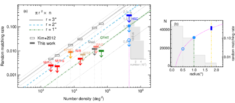
Figure 9: (Left) Random matching rate in terms of the source density and matching radius. The open boxes are taken from the Fig 14 in Kim et al. (2012), which represent the actual tests, i.e., number counts of the sources randomly matched to each data using 3 ^′′ radius. The grey thick line shows these measurements are described by a simple relation ($n\pi r^{2}$). If we use 2^′′ or 1^′′ radius, the random matching rate will be decreased as described by cyan dashed and green dot-dashed lines. The faint dotted lines between them indicate 0.5^′′ increments. The filled boxes in different colours show the random matching estimates when a certain source is matched against the data with our radii determined in this work. The grey histogram is taken from Fig 3d. (Right) The embedded grey histogram on the left panel can be plotted with random matching rate as shown in the right panel. The magenta curve shows the random matching rate when the number density of source is 4.5$\times 10^{5}$ (which corresponds to the magenta vertical line in the left panel). Vertical yellow line represents the matching radius from Figure 3.

3.2 Spectroscopic and Photometric Redshifts

Following the optical identification of the AKARI sources with the deep HSC data, we incorporated all available spectroscopic redshifts (spec-z) data to the clean AKARI-HSC sources (therefore, the redshift information matched to the flagged sources are not included here.). There have been many spectroscopic observations over the AKARI’s NEP area. The most extensive and massive campaign covering the entire NEPW field was done by Shim et al. (2013): they targeted the NEPW sources selected primarily based on the MIR fluxes at 11 $\mu$m ($S11<18.5$ mag) and at 15 $\mu$m ($L15<17.9$ mag) to see the properties of the MIR selected SFGs. Most of these flux-limited sources turned out to be various types of IR luminous populations of galaxies. A smaller number of secondary targets (35$\%$ out of their targets) are also selected to catch some rare types of objects, such as obscured AGNs, BzKs, super cluster candidates, etc. They provided the spectra of 1796 sources (primary targets: 1155, secondary targets: 641), and the redshifts for 1645 sources were measured. These spectroscopic sources are classified into several types (e.g., star, type1 AGN, type2 AGNs, galaxy, unknown). Recently, a new spectroscopic campaign over the whole NEPW area with the MMT/Hectospec has been initiated to carry out a homogeneous survey for the 9 $\mu$m selected galaxies (MMT2020A/B, PI: H. S. Hwang).

We also took the redshift/type information from many other spectroscopic surveys on the NEPD field. For example, Keck/DEIMOS observations were conducted in order to measure the spectroscopic redshift and calibrate photo-zs for MIR galaxies (DEIMOS08) (Takagi et al., 2010), and to measure [OII] luminosity against 8$\mu$m luminosity (DEIMOS11) (Shogaki et al., 2018), and more recently, to check the line emission evidence of AGNs and metallicity diagnostics of SFGs, etc. (DEIMOS14, DEIMOS15, DEIMOS17) (Kim et al., 2018). Another series of spectroscopic observations with Gran Telescope Canarias (GTC)/OSIRIS were carried out between 2014 and 2017 (e.g., GTC7-14AMEX, GTC4-15AMEX, GTC4-15BMEX, and GTC4-17MEX) (Díaz Tello et al., 2017) to see the X-ray signatures of highly obscured and/or Compton-thick (CT) AGNs along with the identification by the Chandra data (Krumpe et al., 2015). Subaru/FMOS spectroscopy was also obtained to investigate the mass-metallicity relation of IR SFGs in the NEP field (Oi et al., 2017). Ohyama et al. (2018) provided the polycyclic aromatic hydrocarbons (PAHs) galaxy sample with redshift measurements through the SPICY projects done by AKARI/slitless spectroscopy. We combined all these redshift information.

Using these spectroscopic redshifts as a calibration sample, Ho et al. (2020) estimated photo-zs using the photometry from $u^{*}$-band to the NIR band (IRAC2 and/or WISE2). They checked photometry by comparing colours/magnitudes to discriminate the unreasonable data so that they could obtain reliable results when they use the software Le PHARE. After the photo-zs were assigned, they presented effective star-galaxy separation scheme based on the $\chi^{2}$ values.

3.3 Supplementary Near-/Mid-IR Data

While the optical data are crucial for identifying the nature of the corresponding AKARI sources, the $J$-, $H$-, and $K$-band data are useful to bridge the gap in wavelength between optical $y$ and $N2$ band. The CFHT/WIRCam covered a limited area, but provided useful $J$- and $K$-band photometry (Oi et al., 2014). The NIR ($J$, $H$) survey that covered almost the entire NEPW area ($\sim$ 5.2 deg²) was done by FLAMINGOS of the Kitt Peak National Observatory (KPNO) 2.1 m telescope although the depth is shallower than WIRcam data (see Figure 1 and 7). For complementary photometry in the near- to mid-IR, we also included the publicly available data taken by Spitzer (Werner et al., 2004) and WISE (Wright et al., 2010). The catalogue by Nayyeri et al. (2018) provides 380,858 sources covering the entire NEPW field ($\sim$ 7 deg²) with higher sensitivity (21.9 and 22.4 mag at the IRAC1 and IRAC2, respectively) and slightly better spatial resolutions compared to the $N3$ and $N4$, which are useful to cross check against the longer wavelength data having larger PSFs (e.g., the SPIRE or SCUBA-2 data).

3.4 FIR/Smm Data from the Herschel and SCUBA-2

Herschel carried out the 0.44 deg² and 9 deg² surveys over the NEP field with the Photoconductor Array Camera and Spectrometer (PACS: Poglitsch et al., 2010) and Spectral and Photometric Imaging REceiver instrument (SPIRE: Griffin et al., 2010), respectively. From the PACS NEP survey (Pearson et al., 2019; Burgarella et al., 2019), the Green (100 $\mu$m) and Red (160 $\mu$m) bands provide 1380 and 630 sources over the NEPD field, with the flux densities of 6 mJy and 19 mJy at the 50% completeness level, respectively. The SPIRE also carried out NEP survey as an open time 2 program (PI: S. Serjeant, in 2012), and completely covered the entire NEPW field, at the 250, 350, and 500 $\mu$m (achieving 9.0, 7.5, and 10.8 mJy sensitivities at each band). Source extraction was carried out on the 250 $\mu$m map, and approximately $\sim$4800 sources were catalogued with the photometry in all three SPIRE bands. The more detailed description of the data reduction and photometry can be found in Pearson et al. (2017). Compared to the optical or NIR data, the Herschel (PACS or SPIRE) data have larger positional uncertainties with much larger PSF sizes. This can make the identification of sources against the AKARI data potentially ambiguous when we carry out the positional matching, even though the radius was determined reasonably (the 3-sigma radii are smaller than the PSF sizes, in general, as shown in Table 2). In our catalogue, the cases that multiple AKARI clean sources are lying within the searching radius around the SPIRE/PACS positions were not included so that we clearly chose only one AKARI counterpart against the Herschel sources. The 850 $\mu$m submilimetre (sub-mm) mapping on the NEPW field is currently ongoing by one of the large programs with the JCMT/SCUBA-2 (Shim et al., 2020). They released a mosaic map and a catalogue for the central 2 deg² area first. They provide 549 sources above 4-$\sigma$ with a depth of 1.0–2.3mJy per beam. The source matching against the AKARI-HSC clean catalogue was carried out based on the likelihood ratio. We derived the probability of counterpart for a 850$\mu$m source, using both the magnitudes distribution of IRAC1 and IRAC2 bands (which are deeper than those of the AKARI NIR bands) and their colour as well as those of three SPIRE bands. We took 46 sources as robust AKARI counterparts for the 850 $\mu$m sources because they are matched to both IRAC and SPIRE with high (95$\%$) probability. We also included 16 sources as decent AKARI counterpart because in these examples there is only one IRAC/SPIRE source within the 850$\mu$m beam. Lastly, 4 sources matched to IRAC with high probablity but we are uncertain about the SPIRE cross-identification. However, when multiple optical sources were associated with any given SPIRE or SCUBA-2 source, if real optical counterpart was already classified as flagged sources, then it could be complicated/a potential issue.

4 The properties of the AKARI sources Identified by HSC Survey Data

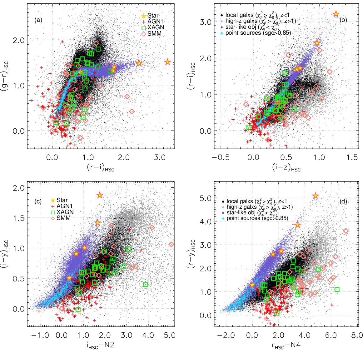
Figure 10: Colour-colour diagrams based on the HSC optical and AKARI NIR bands. Violet dots represent the sources classified as star-like sources, and black dots represent the extra-galactic sources with z${}_{\rm phot}<1$ while the grey dots are the source with z${}_{\rm phot}>1$ (Ho et al., 2020). Cyan dots are high-stellarity (sgc$>0.8$) sources. Yellow stars represent the Galactic stars observed by the spectroscopic survey (Shim et al., 2013). Red crosses are AGNs (type1), also confirmed by Shim et al. (2013). Green boxes are AGNs that have X-ray data (Krumpe et al., 2015; Díaz Tello et al., 2017). Salmon diamons are galaxies observed by the SCUBA-2 survey (Shim et al., 2020). All axes are in units of AB mag.

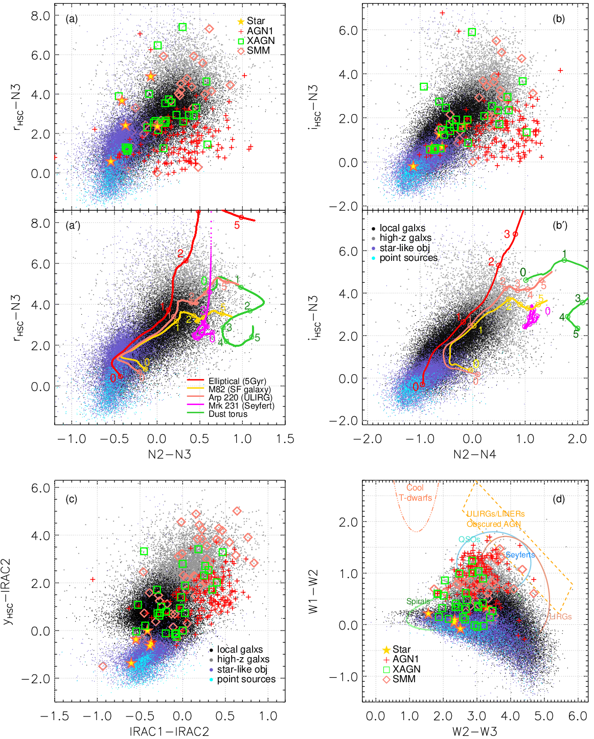
Figure 11: Colour-colour diagrams based on the HSC and various NIR bands (AKARI, Spitzer, and WISE), with the symbols in the same fashion as presented in Figure 10: star-galaxy separation and how their locations change in different colour-colour diagrams are described. For top panels (a and b), we present the evolutionary tracks of several model templates from Polletta et al. (2007). All axes are in units of AB mag except for the lower right panel (d), which is given in units of Vega mag to compare with the diagram from Wright et al. (2010). The mag offsets ($\Delta m$) between AB and Vega system ($m_{\textrm{AB}}=m_{\textrm{Vega}}+\Delta m$) are 2.70, 3.34, 5.17 mag for W1, W2, and W3, respectively.

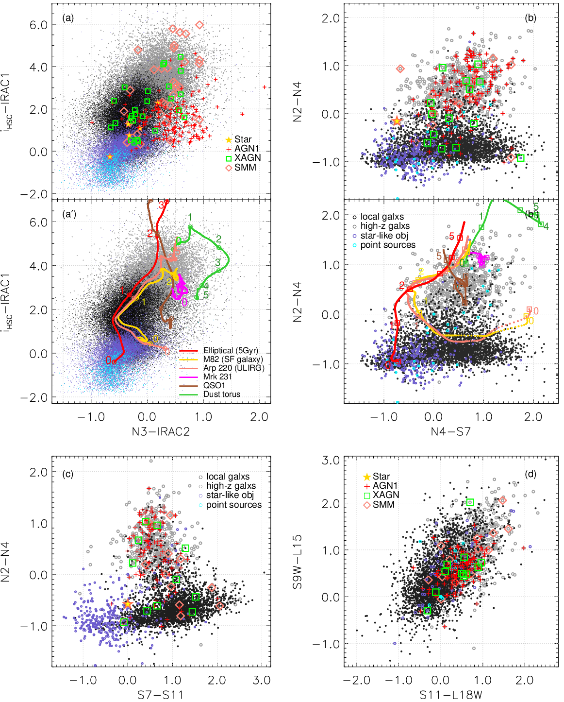
Figure 12: Colour-colour diagrams based on the various combination of NIR to MIR bands, in the same fashion as presented in Figure 10 and 11. Stars begin to fade out in MIR bands. For top panels (a and b), we also present the evolutionary tracks (a^′ and b^′ of several model templates from Polletta et al. (2007). All axes are in units of AB mag

4.1 Overview: reliability vs random matching

When we seek to find a counterpart against a certain data using a searching radius ($r$), there is always a possibility that we could encounter a random source (which is not associated with real counterpart) inside the circle defined by the radius ($\pi r^{2}$). This is the probability that a source can be captured simply by this circular area at any random position of the data. The higher the source density of data we match against, the higher the random matching rate becomes. If we use a larger radius, then the probability is also increased. Kim et al. (2012) showed that it can be expressed in terms of number density ($n$) of data and cross-section. See the open boxes and grey solid lines in Figure 9a, which are taken from the Figure 14 in Kim et al. (2012).

Practically, these have to be regarded as upper limits of a false match possibilities (the worst case), because, in general, two data sets for source matching are correlated with each other: these data are obtained from the same field of view, not from two different arbitrary sky positions. Therefore, the matching results are generally better than this estimation (as indicated by the downward arrows).

To give how to interpret the source matching in a consistent way with Kim et al. (2012), we used the same analyses, using our matching radii determined in sections 2 and 3, and compared with the plots in the previous work. In Kim et al. (2012), they used the uniform radius (3^′′, the open boxes in Figure 9a). In this work, however, the matching radii were chosen based on the mean positional offset of the matched sources between the data. This gives much smaller radii compared to those from Kim et al. (2012), even smaller than the PSF sizes which are also used frequently for matching criteria. In Figure 9a, the highest number density of the HSC data ($\sim 4.5\times 10^{5}$ sources per deg²) seems to have a high random matching (the filled blue box). Here, we should remind that only 5% of the sources are matched outside 1.5^′′ and 82% of the sources are matched within 1^′′, as shown by the grey background histogram, which is the same as Figure 3d (but x- and y-axis are transposed/rotated here). Therefore, the random matching rate is better than the filled circle on the green dot-dashed line. On the right panel (b) in Figure 9, this grey histogram is re-plotted with random matching rate, which gives more straightforward description. However, it should be noted that this is just an estimation of the probability when the test was performed on random positions. Only a small fraction will suffer from the random matching, in reality. The sources matched within 0.^′′5 seem obviously reliable (downward below the open circle). In the same fashion, the matching with the other supplementary data (in green, grey, salmon boxes, and so on), which have a much lower number density, are less affected by random matching and relatively safe compared to the HSC data.

4.2 Colour-colour Diagrams

We describe the photometric properties of the NEPW infrared sources matched to the HSC optical data using various colour-colour diagrams (Figures 10 to 12). The colour-colour diagrams are also helpful to see, from a statistical standpoint, if the source matching was accomplished properly. In each diagram, we used several different colours and symbols to distinguish between the different types of sources. Violet dots indicate the sources classified as star-like, which were fitted better to the stellar model templates rather than the galaxy templates, following the diagnostics ($\chi^{2}_{\rm star}<\chi^{2}_{\rm galaxy}$) by Ilbert et al. (2009) when the photo-z estimation was performed with Le PHARE (Ho et al., 2020). The sources fitted better to the galaxy templates are divided into two groups by redshift: black dots represent the local (z${}_{\rm phot}<1$) galaxies and the grey dots represent the high-z ($>1$) objects. To see if the star-like sources are classified appropriately, we over-plotted (in cyan) the sources having high stellarity (i.e., star-galaxy classifier; sgc$>0.85$ ), measured with the SExtractor on the CFHT data (Hwang et al., 2007; Jeon et al., 2010). The stellar sequence appears prominently in the optical colour space because the stellar SED shows blackbody-like behaviors, which naturally generate a systematically and statistically well-defined sequence.

In our spectroscopic sample (as explained in sec. 3.2), we have various types classified by the line emission diagnostics. We also plotted some of them here: spectroscopically confirmed stars (marked by yellow star), type-1 AGNs (red cross), AGNs identified in X-ray data (green square), as well as the sub-mm galaxies detected in SCUBA-2 survey (salmon diamond).

Figure 10 shows the colour-colour diagrams using the photometry in the HSC and AKARI NIR bands. The violet dots form a well-distinct track, cyan dots are exactly tracing this track, and five spectrocopic stars are overlaid on them. Those star-like sources (as well as the point sources) seem to be the representative of the Galactic stars, but it is obvious that not all of them are stars (i.e., quite a few real galaxies, which just happen to fall on the stellar locus, are included in the vicinity of the sequence). This implies that the source matching was properly achieved and the star-galaxy separation was also effectively done. In the optical colour-colour diagrams, the stellar sequence overlaps with extragalactic sources, positionally entangled with them on the same area (Figure 10a and 10b), but when the NIR bands are involved, this stellar sequence gets separated from the extra-galactic populations (Figure 10c, 10d). In the NIR colour-colour diagrams, however, stars seem to stay together in a rather circular/elliptical area, not in the form of a track (Figure 11). They gradually disappear in the longer wavelengths (Figure 12).

In the optical colour-colour diagrams (Figure 10), the black and grey dots (local and high-z galaxies, respectively) are gathered mostly in the same area, but the grey dots seem to be more widespread. In Figure 11, the black dots seem to be gathering in an apparently different place from the grey dots which are spread towards the redder direction, being consistent with the photo-z classification and implying high-z populations. This separation becomes obvious in $N2-N4$ colour (Figure 12b and 12c), which appears to be a very good selector of high-z objects or AGNs, seemingly related to hot dust heated by energetic sources (Fritz et al., 2006; Lee et al., 2009).

In Figure 11 and 12, we present the redshift tracks ($0<$z$<5.5$) to compare with the colour-colour diagrams based on the HSC and AKARI NIR bands (See Figure 11a^′, 11b^′, 12a^′, and 12b^′). They enable us to seize the characteristics of the sources by comparing the trajectories of typical models with real galaxies observed by the optical-IR surveys (as well as the symbols in the top panels, Figure 11a, 11b, 12a, and 12b). In Figure 12, it should be noted that the model tracks show some overlaps in a certain area suggesting there seems to be partly a mixture of SFGs and AGNs. To select AGN types, the $N2-N4$ colour seems to be more effective when we use a combination with MIR bands (e.g., $N4-S7$ or $S7-S11$).

The AGN types and SMM galaxies stay close to the black/grey dots. It is not easy to discern clear trends. However, the green boxes are widely overlapped with all the extragalacic sources (black and grey dots), while the red crosses (type-1) tend to stay in a specific area, all through the colour-colour diagrams. Salmon diamonds (SMM galaxies) are also spread over the black and grey dots, but more widely spread compared to the green boxes and they seem to prefer to stay around the grey dots, implying the SMM galaxies are more likely to be high-z populations. On the other hand, it would be interesting to see the follow-up studies (e.g., Poliszczuk et al. in prep; Chen et al. in prep) if machine learning algorithms such as the support vector machine or deep neural network, etc. can do more effective separations in various color/parameter spaces (not just in two-dimensional projections of them).

5 Summary and Conclusion

The NEP field has been a long-standing target since it was surveyed by the legacy program of AKARI space telescope (Serjeant et al., 2012). Previous optical surveys (Hwang et al., 2007; Jeon et al., 2010) were incomplete, which was a strong movitation to obtain deep Subaru/HSC optical data covering the entire NEP field (Goto et al., 2017). We achieved the faint detection limits (Oi et al., 2020), which enabled us to identify faint AKARI sources in the near and mid-IR bands, and initiated a variety of new studies. We constructed a band-merged catalogue containing photometric information for 42 bands from UV to the sub-mm 500$\mu$m. The photo-zs for the NEPW sources were derived based on this data with all available redshift information (Ho et al., 2020), and were incorporated into the catalogue as well. We investigated the photometric properties of the NEPW sources observed by the HSC using colour-colour diagrams based on this band-merged catalogue. We are able to roughly see how the shape of stellar sequence changes and which areas the AGN types prefer to stay in different colour spaces, as the observed wavelength increases, although it is difficult to tell about the clear trend of extragalactic populations because none of the quantitative analysis has been made.

This band-merging gives us the benefits of constructing full SEDs for abundant dusty galaxy samples for SED modeling, e.g., using CIGALE (Boquien et al., 2019) or MAGPHYS (da Cunha et al., 2008), especially taking advantage of the uniqueness of the continuous MIR coverage as well as a wide range of panchromatic photometry. It provides more opportunities to disentangle otherwise degenerate properties of galaxies or to excavate hidden information for a better understanding of the physics behind various IR features.

Due to the uniqueness of the filter coverage by AKARI, this legacy data remains the only survey having continuous mid-IR imaging until JWST carries out its first look at the sky. The science on this NEP field is currently driven by Subaru/HSC (Oi et al., 2020), SCUBA-2 (Shim et al., 2020), and homogeneous spectroscopic surveys. Since many future space missions are planning to conduct deep observations of this area – e.g., Euclid (Laureijs et al., 2011), JWST (Gardner et al., 2006), SPHEREx (Doré et al., 2016, 2018), etc., a great deal of synergy is expected together with the legacy data as well as our ongoing campaigns.

Data availability

The band-merged catalogue in this work is available at Zenodo (https://zenodo.org/record/4007668$\#$.X5aG8XX7SuQ). Other data addressed in this work will be shared on reasonable request to the corresponding author.

References

- Aihara et al. (2018) Aihara H. et al., 2018, PASJ, 70, S4
- Barrufet et al. (2020) Barrufet L., Pearson C., Serjeant S., et al., 2020, A&A, 641, A129
- Bertin & Arnouts (1996) Bertin E., & Arnouts S. 1996, A&AS, 117, 393
- Boquien et al. (2019) Boquien M., Burgarella D., Roehlly Y., et al., 2019, A&A, 622, A103
- Bosch et al. (2018) Bosch J., Armstrong R., Bickerton S., et al., 2018, PASJ, 70, S5
- Burgarella et al. (2019) Burgarella D., et al., 2019, PASJ, 71, 12
- Casey et al. (2014) Casey C. M., Narayanan D., & Cooray A., 2014, Phys. Rep., 541, 45
- Chiang et al. (2019) Chiang C-Y., Goto T., Hashimoto T., et al., 2019. PASJ, 71, 31
- da Cunha et al. (2008) da Cunha E., Charlot S., & Elbaz D., 2008
- Díaz Tello et al. (2017) Díaz Tello J., Miyaji T., Ishigaki T., et al., 2017, A&A, 604, A14
- Doré et al. (2016) Doré O., Werner M. W., et al., 2016, arXiv:1606.07039
- Doré et al. (2018) Doré O., Werner M. W., et al., 2018, arXiv:1805.05489
- Fritz et al. (2006) Fritz J., Franceschini A., & Hatziminaoglou E., 2006, MNRAS, 366, 767
- Galliano et al. (2018) Galliano F., Galametz M., & Jones A. P., 2018, ARA&A
- Gardner et al. (2006) Gardner J. P., Mather J. C., et al., 2006, Space Sci. Rev., 123, 485
- Geach et al. (2017) Geach J. E., Dunlop J. S., et al., 2017, MNRAS, 465, 1789
- Goto et al. (2010) Goto T., Takagi T., Matsuhara H, et al., 2010, MNRAS, 514, A6
- Goto et al. (2017) Goto T., Toba Y., Utsumi Y., Oi, N., et al., 2017, PKAS, 32, 225
- Goto et al. (2019) Goto T., Oi N., Utsumi Y., et al., 2019, PASJ, 71, 30
- Griffin et al. (2010) Griffin M. J., Abergel A., Abreu A., et al., 2010, A&A, 518, L3
- Henry et al. (2006) Henry J. P., Mullis C., R., Gioia I. M., & Huchra J. P., 2006, ApJS
- Hickox & Alexander (2018) Hickox R. C., & Alexander D. M., 2018, ARA&A, 56, 625
- Ho et al. (2020) Ho C.-C., Goto T., Oi N., et al., 2020, MNRAS, submitted
- Huang et al. (2018) Huang S., Leauthaud A., Murata R., et al., 2018, PASJ, 70, S6
- Huang et al. (2020) Huang T.-C., Matsuhara H., Goto T., et al. 2020, MNRAS, 498, 609
- Hwang et al. (2007) Hwang H. S., Serjeant S., Lee M. G., 2007, MNRAS, 375, 115
- Hwang et al. (2010) Hwang H. S., Elbaz D., Magdis G., et al., 2010, MNRAS, 409, 75
- Hwang et al. (2012) Hwang H. S., Geller M. J., Kurtz M. J., 2012, A&A, 758, 25
- Hwang et al. (2007) Hwang N., Lee M. G., Lee H. M., et al., 2007, ApJS, 172, 583
- Ilbert et al. (2009) Ilbert O., Capak P., et al., 2009, ApJ, 690, 1236
- Im et al. (2010) Im M., Ko J., Choi Y., et al., 2010, J. Korean Astron. Soc., 43, 75
- Ishihara et al. (2010) Ishihara D., Onaka T., Kataza H., et al., 2010, A&A, 514, 1
- Jarrett et al. (2011) Jarrett T. H., Cohen M., et al., 2011, ApJ, 735, 112
- Jansen & Windhorst (2018) Jansen R. A., & Windhorst R. A., 2018, PASP, 130, 124001
- Jeon et al. (2010) Jeon Y., Im M., Ibrahimov M., et al., 2010, ApJS, 190, 166
- Jeon et al. (2014) Jeon Y., Im M., Kang E., et al., 2014, ApJS, 214, 20
- Holloway (1986) Holloway J., 1986, J. Appl. Phys., 60, 1091
- Kim et al. (2018) Kim H. K., Malkan M. A., et al., 2018, in Ootsubo T., Yamamura I., Murata K., Onaka T., eds, The Cosmic Wheel and the Legacy of the AKARI Archive: From Galaxies and Stars to Planets and Life. pp 371-374
- Kim et al. (2012) Kim S. J., Lee H. M., Matsuhara H., et al., 2012, A&A, 548, A29
- Kim et al (2019) Kim S. J., Jeong W-S., Goto T., et al., 2019, PASJ, 71, 11
- Kirkpatrick et al. (2012) Kirkpatrick et al., 2012, ApJ, 759, 139
- Komatsu et al. (2011) Komatsu E., Smith K. M., Dunkley J., et al., 2011, ApJS, 192, 18
- Krumpe et al. (2015) Krumpe M., Miyaji T., Brunner H., et al., 2015, MNRAS, 446, 911
- Laureijs et al. (2011) Laureijs R. et al., 2011, arXiv:1110.3193
- Lee et al. (2009) Lee H. M., Kim S. J., Im M., et al., 2009, PASJ, 61, 375
- Lutz (2014) Lutz D., 2014, ARA&A, 52, 373
- Madau & Dickinson (2014) Madau P., & Dickinson, M., 2014, ARA&A, 52, 415
- Małek et al. (2014) Małek K., Pollo A., Takeuchi T. T., et al., 2014, A&A, 562, A15
- Matsuhara et al. (2006) Matsuhara H., Wada T., Matsuura S., et al., 2006, PASJ, 58, 673
- Merloni et al. (2012) Merloni A. et al., 2012, arXiv:1209.3114
- Miyazaki et al. (2018) Miyazaki S., Komiyama Y., Kawanomoto S., et al., 2018, PASJ, 70, S1
- Murakami et al. (2007) Murakami H., Baba H., Barthel P., et al., 2007, PASJ, 59, S369
- Nayyeri et al. (2018) Nayyeri H., Ghotbi N., Cooray A., et al., 2018, ApJS, 234, 38
- Offenberg et al. (2001) Offenberg J., Fixen D. J., Fauscher B. J., et al., 2001, PASJ, 113, 240
- Oi et al. (2014) Oi N., Matsuhara H., Murata K, Goto T., et al., 2014, A&A, 566, A60
- Ohyama et al. (2018) Ohyama Y., Wada T., Matsuhara H., Takagi T., et al., 2018, A&A, 618, A101
- Oi et al. (2017) Oi N., Goto T., Malkan M., Pearson C., & Matsuhara H., 2017, PASJ, 69, 70
- Oi et al. (2020) Oi N., Goto T., Matsuhara H., et al., 2020, MNRAS, accepted
- Onaka et al. (2007) Onaka T., Matsuhara H., Wada K., et al., 2007, PASJ, 59, S401
- Pearson et al. (2017) Pearson C., Cheale R., Serjeant S., et al., 2017, PKAS, 32, 219
- Pearson et al. (2019) Pearson C., Barrufet L., Campos Varillas M. d. C., et al., 2019, PASJ, 71, 13
- Pilbratt et al. (2010) Pilbratt G. L., Riedinger J. R., Passvogel T., et al., 2010, A&A, 518, L1
- Poglitsch et al. (2010) Poglitsch A., Waelkens C., Geis N., et al., 2010, A&A, 518, L2
- Poliszczuk et al. (2019) Poliszczuk A., Solarz A., Pollo A., et al., 2019, PASJ, 71, 65
- Polletta et al. (2007) Polletta M. Tajer M., et al., 2007, ApJ, 663, 81
- Sanders et al. (2014) Sanders D. B., 2014 AdSpR, 34, 535
- Serjeant et al. (2012) Serjeant S., et al., 2012, arXiv:1209.3790.
- Shim et al. (2013) Shim H., Im M., Ko J., et al., 2013, ApJS, 207, 37
- Shim et al. (2020) Shim H., Kim Y., Lee D., Lee H. M., 2020, MNRAS, 498, 5065
- Shogaki et al. (2018) Shogaki A., Matsuura S., et al., 2018, in Ootsubo T., Yamamura I., Murata K. Onaka T., eds, The Cosmic Wheel and the Legacy of the AKARI Archive: From Galaxies and Stars to Planets and Life. pp 367-370
- Spergel et al. (2015) Spergel D., Gehrels N. et al., 2015, arXiv:1503.03757
- Sutherland & Saunders (1992) Sutherland W. & Saunders W., 1992, MNRAS
- Takagi et al. (2010) Takagi T., Oyama Y., Goto T., et al., 2010, A&A, 514, A5
- Takagi et al. (2012) Takagi T., Matsuhara H., Goto T., Hanami H., et al., 2012, A&A, 537, A24
- Toba et al. (2015) Toba Y., Nagao T., Strauss M. A., et al., 2015, PASJ, 67, 86
- Toba et al. (2020) Toba Y., Goto T., Oi N., Wang T. -W., Kim S. J., et al., 2020, ApJ, 899, 35
- Wada et al. (2008) Wada T., Matsuhara H., Oyabu S., et al., 2008, PASJ, 60, S517
- Wang et al. (2020) Wang T.-W., Goto T., Kim S. J., et al., 2020, MNRAS, accepted
- Werner et al. (2004) Werner M. W., Roellig T. L., Low F. J., et al., 2004, ApJS, 154, 1
- White et al. (2017) White G. J., Barrufet Laia, et al., 2017, PKAS, 32, 231
- White et al. (2010) White G. J., Pearson C., Braun R., et al., 2010, A&A, 517, A54
- Wright et al. (2010) Wright E. L., Eisenhardt P. R. M., Mainzer A. K., et al., 2010, AJ, 140, 1868