On the Gaussian Approximation to Bayesian Posterior Distributions

Abstract

The present article derives the minimal number $N$ of observations needed to consider a Bayesian posterior distribution as Gaussian. Two examples are presented. Within one of them, a chi-squared distribution, the observable $x$ as well as the parameter $\xi$ are defined all over the real axis, in the other one, the binomial distribution, the observable $x$ is an entire number while the parameter $\xi$ is defined on a finite interval of the real axis. The required minimal $N$ is high in the first case and low for the binomial model. In both cases the precise definition of the measure $\mu$ on the scale of $\xi$ is crucial.

Keywords Bayesian posterior  $\cdot$ Gaussian approximation  $\cdot$ chi-squared and binomial distributions

1 General Notions and Definitions

Bayesian statistics distinguishes the observations $x_{1}\,,\dots\,,x_{N}\,$ from the parameter $\xi$ that “conditions” them. Bayes’ theorem — given below — expresses the uncertainty about $\xi$ via a probability distribution of $\xi$ conditioned by the observations $x_{1}\,,\dots\,,x_{N}\,.$ This so-called posterior distribution becomes always narrower with increasing $N\,.$ By consequence the “true value” of $\xi$ is approached more and more closely. Simultaneously the posterior approaches a Gaussian distribution. This is a consequence of the fact that the posterior after $N$ observations becomes the $N$-th power of the posterior from one observation.

The present article, based on Bayesian statistics, derives the minimal $N$ needed for the Gaussian approximation. In the first part, comprising Sects. 2 and 3, the variables $x$ and $\xi$ are defined along the real axis as a whole. A chi-squared distribution provides an example. In the second part, i.e. in Sects. 4 and 5, the parameter $\xi$ is defined on a finite interval of the real axis. The so-called trigonometric distribution serves as example.

We explain some notions used throughout the following text.

A statistical model $p(x|\xi)$ formulates the relation between the observations $x$ and the parameter $\xi\,.$ A statistical model is normalised according to

$$\int_{domain\,x}{\rm d}x\,p(x|\xi)\,=\,1$$ (1)

for every $\xi\,.$ Here, “$domain\,x$” means that the integral extends over the domain of definition of the observed $x\,.$

Bayes’ theorem [4] states the posterior distribution

$$P(\xi|x)\,=\,\frac{p(x|\xi)\mu(\xi)}{m(x)}\,,$$ (2)

of $\xi$ conditioned by $x\,.$ The Bayesian prior distribution $\mu(\xi)$ serves also as the measure of integration over $\xi\,,$ see Eq. (33) and the explanation there. The quantity

$$m(x)\,=\,\int_{domain\,\xi}{\rm d}\xi\,p(x|\xi)\mu(\xi)$$ (3)

normalises $P(x|\xi)$ to unity. Equation (2) gives the posterior in the case of a single observation $x\,.$ There is usually more than one observation, but in the present text there shall be only one parameter $\xi\,.$ For the case of $N$ observations $\mathbb{x}=(x_{1},\dots,x_{N})$ the posterior is formulated in Sects. 2.4 and 4.4.

The Fisher information [16, 17, 18, 19] is the expectation value

$$F(\xi)\,=\,\int_{domain\,x}{\rm d}x\,p(x|\xi)\left[\frac{\partial}{\partial\xi}\ln p(x|\xi)\right]^{2}$$ (4)

of the quantity $[\partial/\partial\xi\,\ln p(x|\xi)]^{2}\,.$ The Fisher information is always positive. When $p$ is a Gaussian distribution then $F$ is the inverse of the mean square value of the Gaussian.

Form invariance is a symmetry relation between the observation $x$ and the condition $\xi\,.$ It is defined by a group — in the sense of the theory of Lie groups [24, 32] — of transformations that leave $p(x|\xi)$ unchanged when applied to both, $x$ and $\xi\,.$ See Chap. 6 of [25] and the textbooks [1, 7].

In the examples of the present text the symmetry shows up by the fact that the model $p(x|\xi)$ depends on the difference $x-\xi\,.$ The symmetry group then consists of all possible simultaneous translations of $x$ and $\xi$ by the same shift. Many statistical models can be reformulated such as to display translational form invariance. In section 2 the details of translational form invariance are discussed. It is taken as the starting point for a Gaussian approximation to the posterior distribution since the Gaussian itself is form invariant under translations. The invariant measure of the group of translations is identified with the prior distribution. Here, this implies

$$\mu(\xi)\,\equiv\,{\rm const}\,.$$ (5)

In Sects. 2 and 4 two different cases are considered: Continuous $x$ and $\xi$ within a chi-squared model and dichotomic $x$ within the binomial model. Both cases are widespread and of practical interest for many applications.

A likelihood function ${\cal L}_{N}(\xi)$ is proportional to the probability density $p_{N}(\mathbb{x}|\xi)$ of $N$ observations $\mathbb{x}$ considered as a function of $\xi$ while $\mathbb{x}$ is given. When — in the present context of Eq. (5) — the domain of definition of $\xi$ extends over the whole real axis, the likelihood function possesses a maximum: Since the posterior is normalised, it must tend to zero when $\xi$ goes to infinity.

The value $\xi^{\rm ML}$ where the maximum occurs, is called the maximum likelihood or ML estimator of the “true value” of $\xi\,.$ For every series of observations $\mathbb{x}$ there is a ML estimator $\xi^{\rm ML}=\xi^{\rm ML}(\mathbb{x})\,.$ In sections 2.4 and 4.4 one shall see that $\xi^{\rm ML}$ is the sufficient statistic [37] of the model — a notion widely discussed in the development of the Rasch model [53, 49, 55, 13, 14, 21, 25].

It might appear that the constancy of the prior is nothing but the "principle of indifference", well-known in the history of statistical and Bayesian reasoning, well-known also for its difficulties when applied to transform probability densities [11, 20]. Note that in the present paper the constancy of the prior occurs as a consequence of the well-defined group theoretical property of “form invariance” [26].

In Sects. 3.1 and 5 the likelihood function of a model $p(x|\xi)$ is compared to the Gaussian model

$$G(x|\xi)\,=\,(2\pi\sigma^{2})^{-1/2}\exp\left(-\frac{(x-\xi)^{2}}{2\sigma^{2}}\right)\,,\quad\quad-\infty<x,\xi<\infty\,.$$ (6)

The $N$-fold Gaussian model, i.e. the distribution of $N$ observations $\mathbb{x}=(x_{1},\dots,x_{N})\,,$ is

$$G_{N}(\mathbb{x}|\xi)\,=\,\left(\frac{1}{2\pi\sigma^{2}}\right)^{N/2}\prod_{k=1}^{N}\,\exp\left(-\frac{(x_{k}-\xi)^{2}}{2\sigma^{2}}\right)\,.$$ (7)

This yields the posterior distribution

$$G_{N}(\xi|\mathbb{x})\,=\,\left(\frac{N}{2\pi\sigma^{2}}\right)^{1/2}\exp\left(-\frac{N}{2\sigma^{2}}(<x>-\xi)^{2}\right)\,,$$ (8)

where $<x>$ is the average

$$<x>\,=\,\frac{1}{N}\sum_{k=1}^{N}\,x_{k}\,,$$ (9)

see appendix I. The Fisher information of the Gaussian (6) is

$$F^{\rm Gauss}\,\equiv\,\sigma^{-2}\,.$$ (10)

With increasing number $N$ of observations the posterior of any model $p$ with the prior (5) assumes the Gaussian form and becomes always narrower tending towards Dirac’s delta distribution. We shall determine the minimal $N$ which allows to approximate a given posterior by the Gaussian (8) within the interval $|\xi^{\rm ML}-\xi|<3\sigma/\sqrt{N}\,.$ This interval contains $99.73$ percent of the area under the Gaussian function. Two examples are studied, the chi-squared model in Sect. 3 and the binomial model in Sect. 5. In the two cases the minimal $N$ strongly differ.

2 Form Invariance Along the Real Axis

The present section considers a statistical model $p(x|\xi)$ where both, the observable $x$ and the parameter $\xi\,,$ are defined all along the real axis. Furthermore, $x$ and $\xi$ shall be related via form invariance. These two properties allow a general approximation to the logarithmic likelihood function which contains the sum over $\ln p(x_{k}-\xi)\,.$ These logarithms are $N$ random numbers since the $x_{k}$ are random, whence the sum over the $\ln p(x_{k}-\xi)$ will have a Gaussian distribution for sufficiently large $N\,.$ Yet the central limit theorem does not allow to answer the question, how large $N$ must be for the Gaussian approximation to apply. However, the sum over the $\ln p(x_{k}-\xi)$ becomes equal to the $N$-fold (negative) Kullback-Leibler divergence $H(\xi^{\rm ML}|\xi)\,,$ see Ref. [38] and Eq. (24). The Kullback-Leibler divergence is a quantity that measures the distance between the distributions $p(x|\xi^{\rm ML})$ and $p(x|\xi)\,.$ It will be represented by a Taylor expansion with respect to $\xi\,.$ With increasing $N$ its terms of higher order become negligible as compared to the term of second order. This leads to the criterion for the Gaussian approximation.

2.1 The prior distribution

The above-mentioned two properties of the model $p(x|\xi)$ entail that $p$ depends on the difference $x-\xi$ and only on this difference. Thus the model reads

$$p(x|\xi)\,=\,p(x-\xi)\,,\quad\quad-\infty<x,\xi<\infty\,.$$ (11)

Neither Bayes [4] nor Laplace [39] who independently established Bayes’ theorem, gave a prescription to obtain the prior distribution. Form invariance gives us the prescription: The prior shall be invariant under the symmetry group of translations [32, 34, 35, 25].

Under the translation

$$\xi^{\prime}\,=\,\xi+a$$ (12)

the prior transforms as a density, i.e. $\mu(\xi)$ goes over into

$$\mu_{T}\, = \,\mu(\xi^{\prime}-a)\left|\frac{{\rm d}\xi}{{\rm d}\xi^{\prime}}\right|$$ (13)

$$= \,\mu(\xi^{\prime}-a)\,.$$

This shall be independent of $a\,;$ thus $\mu$ is constant as foreseen in Eq. (5). See also Eq. (33) in Sect. 2.3.

For $N$ events $\mathbb{x}\,,$ conditioned by one and the same value of $\xi\,,$ the model is

$$p_{N}(\mathbb{x}|\xi)\,=\,\prod_{k=1}^{N}\,p(x_{k}-\xi)\,,\quad\quad-\infty<x_{k},\xi<\infty\,.$$ (14)

The posterior is

$$P_{N}(\xi|\mathbb{x})\,=\,\mu(\xi)\frac{\prod_{k=1}^{N}\,p(x_{k}-\xi)}{m(\mathbb{x})}\,,$$ (15)

where

$$m(\mathbb{x})\,=\,\int_{-\infty}^{\infty}{\rm d}\xi\,\mu(\xi)\prod_{k=1}^{N}\,p(x_{k}-\xi)\,.$$ (16)

Since $\mu$ is constant its value drops out of the posterior and $P$ becomes

$$P_{N}(\xi|\mathbb{x})\,=\,\frac{\prod_{k=1}^{N}\,p(x_{k}-\xi)}{\int_{-\infty}^{\infty}{\rm d}\xi^{\prime}\,\prod_{k=1}^{N}\,p(x_{k}-\xi^{\prime})}\,.$$ (17)

One can numerically calculate this expression, determine the shortest interval in which $\xi$ is found with the probability of $99.73$ percent, and thus obtain an error interval for $\xi\,,$ see Chap. 3 of [25]. In Sect. 2.4 this procedure is replaced by considering the logarithm of the likelihood function. This will show that the posterior $P_{N}$ of Eq. (17) tends towards a Gaussian with increasing $N\,.$

2.2 The Maximum-Likelihood Estimator

The expression $p_{N}(\mathbb{x}|\xi)$ of Eq. (14) is called a likelihood function ${\cal L}_{N}(\xi)$ when it is considered as a function of $\xi\,,$ while $\mathbb{x}$ is given.

A likelihood function in the context of translational invariance possesses a maximum since it is a normalisable function defined all along the real axis. When there are several maxima, one must look for the absolute maximum or even redefine the model such that there is an absolute maximum. The place $\xi^{\rm ML}\,,$ where the maximum occurs, depends on the observed $\mathbb{x}\,.$ Hence, $\xi^{\rm ML}=\xi^{\rm ML}(\mathbb{x})$ is a function of $\mathbb{x}\,.$ The value $\xi^{\rm ML}$ is called the maximum likelihood (ML) estimator of the parameter $\xi\,.$ For the example of the chi-squared model in Sect. 3.2 the ML estimator is given in appendix B.

The ML estimator has been introduced by R.A. Fisher [15, 16, 2]. It estimates the “true value” of $\xi$ which conditions the observations $\mathbb{x}\,.$ For every finite $N\,,$ however, the true value remains hidden. With $N\to\infty$ the ML estimator converges to it. An example is given by the Gaussian model (7); the average (9) is its ML estimator.

Section 2.4 shows that $\xi^{\rm ML}(\mathbb{x})$ is the sufficient statistic of the model $p\,,$ i.e. the observations $\mathbb{x}$ enter into the posterior distribution only via $\xi^{\rm ML}\,.$ Compare page 22 of [36] and Sect. 3.1.3 of [21] and chapters 2 and 3 of Ref. [25].

Neyman and Scott [45] have argued against ML estimation. Their argument says that a bias may remain between the expectation value of $\xi$ and the ML estimator. This has caused a considerable debate [58, 56]. The argument of Neyman and Scott is bound to the distinction between between a “structural” and an “incidental” parameter. The model they studied, is form invariant which means that there is a Lie group of transformations that leaves it invariant. Each of the two parameters describes a subgroup. The elements of the different subgroups do not commute with each other. One of the subgroups describes translations, the other one describes dilations, see, e.g., Sect. 7.3 of [25]. The present article describes a more basic situation. We also have two parameters; however, the present subgroups are identical. Both are translational.

At least in the present context of translational form invariance such a bias becomes arbitrarily small with increasing $N$ — as is shown for the chi-squared model of Eq. (45) in Sect. 3.2. It possesses such a bias; but the fact that the posterior tends to a Gaussian with increasing $N$ implies that the bias goes to zero. Future research sould show whether this holds also for the model discussed by Neyman and Scott.

We study the transition of the posterior to a Gaussian distribution by help of the logarithm of $P_{N}$ given in Eq. (15). Since both, $\mu(\xi)$ and $m(\mathbb{x})\,,$ are independent of $\xi\,,$ this likelihood function is proportional to the product of the $p(x_{k}-\xi)\,,$ i.e.

$${\cal L}_{N}(\xi)\,\propto\,\prod_{k=1}^{N}\,p(x_{k}-\xi)\,.$$ (18)

Therefore the logarithm of ${\cal L}_{N}$ is — up to an additive constant — the sum over the logarithms $\ln p(x_{k}-\xi)\,,$

$${\rm const}+\ln{\cal L}_{N}(\xi)\,=\,\sum_{k=1}^{N}\,\ln p(x_{k}-\xi)\,.$$ (19)

For sufficiently large $N$ the sum over the logarithms is expressed by the expectation value of $\ln p(x-\xi)$ which in principle requires

$${\rm const}+\ln{\cal L}_{N}(\xi)\,=\,N\int_{\infty}^{\infty}{\rm d}x\,p(x-\xi^{\rm true})\ln p(x-\xi)\,.$$ (20)

This integral is the expectation value of $\ln p(x-\xi)$ taken with the distribution conditioned by the “true value” of $\xi\,.$ Jaynes and Bretthorst [31] have called it the “asymptotic” likelihood function, asymptotic in the sense of $N\to\infty\,.$ The true value of $\xi$ remains, however, hidden for every finite $N\,.$ We replace it by the ML estimator $\xi^{\rm ML}$ obtained from the observations $\mathbb{x}=(x_{1},\dots,x_{N})\,.$ Then the “asymptotic” likelihood function becomes

$${\rm const}+\ln{\cal L}_{N}(\xi)\,=\,N\int_{\infty}^{\infty}{\rm d}x\,p(x-\xi^{\rm ML})\ln p(x-\xi)\,.$$ (21)

We want to define $\rm const$ such that $\ln{\cal L}_{N}$ becomes a Kullback-Leibler distance. This is reached when $\rm const$ is set to

$${\rm const}\,=\,-N\int_{\infty}^{\infty}{\rm d}x\,p(x-\xi^{\rm ML})\ln p(x-\xi^{\rm ML})$$ (22)

Then the “asymptotic” likelihood function becomes

$$\ln{\cal L}_{N}(\xi)\,=\,N\int_{{\rm domain}\,x}{\rm d}x\,p(x-\xi^{\rm ML})\ln\frac{p(x-\xi)}{p(x-\xi^{\rm ML})}\,.$$ (23)

We call this integral the functional

$$H(\xi^{\rm ML}|\xi)\,=\,\int_{{\rm domain}\,x}{\rm d}x\,p(x-\xi^{\rm ML})\ln\frac{p(x-\xi)}{p(x-\xi^{\rm ML})}\,.$$ (24)

It is the negative of the Kullback-Leibler divergence [38, 27, 9] between the distributions conditioned by $\xi^{\rm ML}$ and by $\xi\,.$ Thus the logarithmic likelihood function becomes

$$\ln{\cal L}_{N}(\xi)\,=\,N\,H(\xi^{\rm ML}|\xi)\,.$$ (25)

The Taylor expansion of $H$ with respect to $\xi$ will yield our criterion by requiring that terms of higher than the second order be negligible.

How large must $N$ be for $\ln{\cal L}_{N}$ to become equal to the expectation value (23)? We follow the assumption that there is such an $N\,.$ For this and larger $N$ equation (23) holds: The logarithmic likelihood function of the Gaussian (8) is

$$\ln{\cal L}_{N}^{\rm Gauss}(\xi)\,=\,N\left[-\frac{(<x>-\xi)^{2}}{2\sigma^{2}}\right]\,,$$ (26)

where the quantity in rectangular brackets is the functional (24) for the Gaussian (6),

$$H^{\rm Gauss}(\xi^{\rm ML}|\xi)\,=\,-\frac{(<x>-\xi)^{2}}{2\sigma^{2}}\,.$$ (27)

The quantity $<x>\,,$ given in Eq. (9), is the ML estimator of the Gaussian model. One sees that Eqs.  (21) and (25) are fulfilled by the Gaussian model.

Equation (103) in appendix A shows that the maximum value of $H(\xi^{\rm ML}|\xi)$ — and thus of the logarithmic likelihood — occurs at $\xi=\xi^{\rm ML}$ for every distribution of the form $p(x-\xi)\,.$

According to Eq. (25) the likelihood ${\cal L}_{N}(\xi)$ has the form of the $N$-th power of ${\cal L}_{N=1}(\xi)$ since $\ln{\cal L}_{N}(\xi)$ is proprotional to $N\,.$ The translational invariance of $p$ given by Eq. (11) leads to a translational invariance of $H$ since

$$H(\xi^{\rm ML}|\xi)\, = \,\int_{-\infty}^{\infty}{\rm d}x\,p(x-\xi^{\rm ML})\ln\frac{p(x-\xi)}{p(x-\xi^{\rm ML})}$$ (28)

$$= \,\int_{-\infty}^{\infty}{\rm d}x^{\prime}\,p(x^{\prime}-\xi^{\rm ML}+\xi)\ln\frac{p(x^{\prime})}{p(x^{\prime}-\xi^{\rm ML}+\xi)}$$

$$= \,H(\xi^{\rm ML}-\xi)|0)\,.$$

This result has been obtained by substituting

$$x^{\prime}\,=\,x-\xi\,.$$ (29)

Thus $H(\xi^{\rm ML}|\xi)$ depends on the difference $\xi^{\rm ML}-\xi$ and only on this difference.

When there are isolated points where $p(x^{\prime})$ or $p(x^{\prime}-\xi^{\rm ML}+\xi)$ vanish, then appendix H shows that the integral exists despite the divergence of the integrand in (28).

2.3 The Fisher Information

The information that carries the name of R.A. Fisher [17] is a central concept of statistics and estimation theory. It provides the prior, if form invariance holds. The Fisher information $F$ is defined as the expectation value of the squared derivative of the logarithmic likelihood function, see Refs. [16, 17, 18, 19] and Sect. 4.2 of [21], i.e.

$$F(\xi)\, = \,\int_{domain\,x}{\rm d}x\,p(x|\xi)\left[\frac{\partial}{\partial\xi}\ln p(x|\xi)\right]^{2}$$ (30)

$$= \,-\int_{domain\,x}{\rm d}x\,p(x|\xi)\frac{\partial^{2}}{\partial\xi^{2}}\ln p(x|\xi)\,.$$

The two expressions equal each other because $p$ is normalised to unity for every $\xi\,,$ see appendix C. Note that the definition (30) refers to a single observation, see [42]. Other authors, however, define the Fisher information for multiple observations [47]. The integration in (30) extends over the full domain of definition of $x\,.$ Given the domain of Eq. (11) one has by use of the substitution (29)

$$F\, = \,-\int_{-\infty}^{\infty}{\rm d}x\,p(x-\xi)\frac{\partial^{2}}{\partial\xi^{2}}\ln p(x-\xi)$$ (31)

$$= \,-\int_{-\infty}^{\infty}{\rm d}x^{\prime}\,p(x^{\prime})\frac{{\rm d}^{2}}{{\rm d}{x^{\prime}}^{2}}\ln p(x^{\prime})\,.$$

Thus the Fisher information of the model (11) is independent of $\xi\,.$ This is a consequence of form invariance under translations.

By the definitions of $H$ in (24) and $F$ in (30) one recognises that

$$F\,=\,-\left.\frac{\partial^{2}}{\partial\xi^{2}}H(\xi^{\rm ML}|\xi)\right|_{\xi=\xi^{\rm ML}}\,.$$ (32)

Since $F$ is positive, the second derivative of $H$ is seen to be negative at $\xi=\xi^{\rm ML}\,.$ This means that the second derivative of ${\cal L}(\xi)$ is negative, as it should be at a maximum.

The prior distribution $\mu$ is proportional to the square root of $F\,,$

$$\mu\,\propto\,\sqrt{F}\,,$$ (33)

according to Hartigan [26] and Jaynes [30]. A measure is the inverse unit of length on the scale of $\xi\,.$

By identifying the integration measure on the scale of $\xi$ with the Bayesian prior distribution, we follow Jeffreys [32] as was done by other authors [33, 29, 35, 48]. The prior is independent of $N\,.$ Since it is independent of $\xi$ and $\xi^{\rm ML}\,,$ a given difference $\xi^{\rm ML}-\xi$ describes the same length of way everywhere on the scale of $\xi\,.$ See also [3, 5, 60, 59, 25] and the footnote .

2.4 The Posterior of a Form Invariant Model

>From Eq. (25) and the fact that the prior is constant follows that the posterior distribution is

$$P_{N}(\xi|\mathbb{x})\,=\,{\cal N}_{N}\exp\Big{(}NH(\xi^{\rm ML}|\xi)\Big{)}\,,$$ (34)

where ${\cal N}_{N}$ normalises $P_{N}$ to unity. The posterior from $N$ observations has the form of the $N$-th power of the posterior for $N=1\,.$ Therefore with increasing $N$ the posterior is more and more restricted to the immediate neighborhood of the maximum at $\xi=\xi^{\rm ML}\,.$ At this maximum $H(\xi^{\rm ML}|\xi^{\rm ML})$ vanishes, since $H$ equals the Kullback-Leibler distance between the distributions $p(x-\xi^{\rm ML})$ and $p(x-\xi)\,.$ Thus for $\xi=\xi^{\rm ML}$ the exponential in (34) has the value of unity,

$$\exp\left(NH(\xi^{\rm ML}|\xi^{\rm ML})\right)\,=\,1\,.$$ (35)

With increasing $N$ the curvature of the likelihood function $\exp(NH(\xi^{\rm ML}|\xi))$ at its maximum increases according to $NF\,,$ were $F$ is the Fisher information at $N=1\,.$ The Fisher information is independent of $\xi$ in the present context. Thus the likelihood function behaves as the Gaussian (8), see Eqs. (26) and (27). It does so in a suitable interval around the maximum value (35) of the likelihood. Thus within that interval the likelihood becomes a Gaussian function.

One also sees that the posterior depends on the observations $\mathbb{x}$ via and only via the estimator $\xi^{\rm ML}=\xi^{\rm ML}(\mathbb{x})\,;$ this means that $\xi^{\rm ML}(\mathbb{x})$ is the sufficient statistic [36]. The notion of sufficient statistic has been widely discussed in the development of the Rasch model of item response theory [53, 49, 13, 14, 55, 21, 25]. We shall come to it in Sect. 4.5 where the binomial model is treated.

3 The Criterion for the Gaussian Approximation

A criterion will now be formulated that allows to find the minimal $N$ so that the Gaussian distribution (8) can be accepted as approximating the posterior $P_{N}$ in Eq. (34).

The Gaussian approximation is justified whenever the Taylor expansion of $\ln{\cal L}_{N}(\xi)$ up to the second order in $\xi$ is “sufficiently precise”. This is the expansion of $H(\xi^{\rm ML}|\xi)$ with respect to $\xi$ at the point $\xi=\xi^{\rm ML}\,.$ In Sect. 3.1 the Taylor expansion is written down and our understanding of “sufficiently precise” is defined. This yields the desired criterion. In Sect. 3.2, the criterion is applied to a chi-squared model.

3.1 Formulation of the Criterion

The Taylor expansion of $H$ up to an arbitrary order $n$ is

$$H(\xi^{\rm ML}|\xi)\,=\,\sum_{\nu=1}^{n}\,\frac{(\xi-\xi^{\rm ML})^{\nu}}{\nu!}\left.\left[\frac{\partial^{\nu}}{\partial\xi^{\nu}}H(\xi^{\rm ML}|\xi)\right]\right|_{\xi=\xi^{\rm ML}}\,+\,R\,.$$ (36)

The quantity $R$ is the remainder. The zero-th order, $\nu=0\,,$ of this expansion vanishes. We expand up to $n=2$ and choose Lagrange’s remainder among several versions suggested in Sect. 0.317 of [22]. This is

$$R\,=\,\frac{(\xi-\xi^{\rm ML})^{3}}{3!}\left.\frac{\partial^{3}}{\partial\xi^{\prime 3}}H(\xi^{\rm ML}|\xi^{\prime})\right|_{\xi^{\prime}=\xi^{\rm ML}+(\xi-\xi^{\rm ML})\Theta}\,,\quad 0<\Theta<1\,.$$ (37)

The value of $\Theta$ remains open except for the fact that it lies between $0$ and $1\,.$

After $N$ observations the Gaussian (8) is accepted as a valid approximation if the remainder $R$ is negligible for all $\xi-\xi^{\rm ML}$ in the interval

$$-3\sigma\frac{1}{\sqrt{N}}\,<\,\xi-\xi^{\rm ML}\,<\,3\sigma\frac{1}{\sqrt{N}}\,.$$ (38)

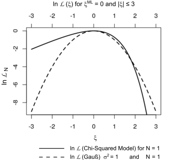
Figure 1: The graph compares a logarithmic likelihood function of a Chi-squared model to that of a Gaussian (i.e. a parabola). The former is taken from Eq. (25) together with (49) and $N=1\,;$ the latter taken from (27) with $\sigma^{2}=F=1\,.$ The likelihood function of a Chi-squared model has a considerable skewness as compared to the Gaussian which is symmetric with respect to $\xi^{\rm ML}-\xi=0\,.$ The figure illustrates that skewness.

containing $99.73$ percent of the area of the Gaussian function. We call it the $3\sigma$-interval of the Gaussian approximation (8), See FIG. 1. The value of $\sigma$ is given by the Fisher information

$$F\,=\,\sigma^{-2}$$ (39)

of the model $p\,.$ This value is the expected curvature of the likelihood function. The Fisher information together with the measure $\mu$ has been defined in Sect. 2.3.

The term of $\nu=0$ in the expansion (36) vanishes according to the definition (24) of the functional $H\,.$ The first derivative $\frac{\partial}{\partial\xi}H$ vanishes at $\xi=\xi^{\rm ML}$ because $H$ attains its maximum value for $\xi=\xi^{\rm ML}\,.$ The second derivative $\frac{\partial^{2}}{\partial\xi^{2}}H$ at $\xi=\xi^{\rm ML}$ yields the negative Fisher information according to Eq. (32). The third derivative — in the remainder — is calculated by help of the translational invariance (28) of H. This gives

$$\left.\frac{\partial^{3}}{\partial\xi^{\prime 3}}H(\xi^{\rm ML}|\xi^{\prime})\right.|_{\xi^{\prime}=\xi^{\rm ML}+(\xi-\xi^{\rm ML})\Theta}\, = \,\left.\int_{-\infty}^{\infty}{\rm d}x\,p(x-\xi^{\rm ML})\frac{\partial^{3}}{\partial\xi^{\prime 3}}\ln p(x-\xi^{\prime})\right.|_{\dots}$$

$$= \,-\left.\int_{-\infty}^{\infty}{\rm d}x\,\frac{\partial^{3}}{\partial\xi^{\prime 3}}p(x-\xi^{\rm ML}+\xi^{\prime})\ln p(x)\right.|_{\dots}$$ (40)

The subscripts $|_{\dots}$ in the r.h.s. of this equation mean repetitions of the subscript on the l.h.s.

In order to decide whether the remainder $R$ is small enough to be neglected, we must find below the largest absolute value $|H^{(3)}|_{\rm max}$ of (40). The largest value of $(\xi-\xi^{\rm ML})^{3}$ occurs at the upper end of the interval (38), whence the maximum absolute value of the remainder is

$$|R|_{\rm max}\,=\,\frac{1}{3!}\left(\frac{3\sigma}{\sqrt{N}}\right)^{3}\,|H^{(3)}|_{\rm max}\,.$$ (41)

This shall be small compared to the second-order-term

$$\frac{1}{2}\left(\frac{3\sigma}{\sqrt{N}}\right)^{2}\,F$$

everywhere in the interval (38). Thus we require

$$\frac{1}{2}\left(\frac{3\sigma}{\sqrt{N}}\right)^{2}\,F\,\gg\,\frac{1}{6}\left(\frac{3\sigma}{\sqrt{N}}\right)^{3}\,|H^{(3)}|_{\rm max}\,.$$ (42)

This gives, by use of (39),

$$1\,\gg\,\frac{|H^{(3)}|_{\rm max}}{N^{1/2}F^{3/2}}\,.$$ (43)

We consider this condition to be fulfilled if

$$0.1\,\geq\,\frac{|H^{(3)}|_{\rm max}}{N^{1/2}F^{3/2}}\,.$$ (44)

The last unequality is our criterion for the validity of the Gaussian approximation. Replacing the requirement (43) by (44), we follow a convention. A step of one “order of magnitude” is usually considered to realise the requirement that one object be large compared to another one.

3.2 The Chi-Squared Model

As an example let us consider the model

$$p(x-\xi)\,=\,\exp\left(x-\xi-e^{x-\xi}\right)\,,\quad\quad-\infty<x,\xi<\infty\,.$$ (45)

It is normalised to unity, see section 8.312, no. 10 of [22]. This is a chi-squared distribution with two degrees of freedom transformed such that it depends on the difference $x-\xi$ between event and parameter, see Eq. (114) in appendix D. The ML estimator is $\xi^{\rm ML}=x\,,$ see Eq. (106) in appendix B.

In the expansion (36) the terms of order $\nu=0,1$ vanish according to Sect. 3.1. The derivatives of $H$ are obtained as follows. The first line of (28) with (45) gives

$$\frac{\partial}{\partial\xi}H(\xi^{\rm ML}|\xi)\, = \,\frac{\partial}{\partial\xi}\int_{-\infty}^{\infty}{\rm d}x\,\Bigl{(}\exp(x-\xi^{\rm ML}-e^{x-\xi^{\rm ML}})\Bigr{)}\left[\xi^{\rm ML}-\xi-e^{x-\xi}+e^{x-\xi^{\rm ML}}\right]$$ (46)

$$= \,\int_{-\infty}^{\infty}{\rm d}x\,\Bigl{(}\exp(x-\xi^{\rm ML}-e^{x-\xi^{\rm ML}})\Bigr{)}\Bigl{[}-1+e^{x-\xi}\Bigr{]}$$

$$= \,-\int_{-\infty}^{\infty}{\rm d}x\,\exp\bigl{(}x-\xi^{\rm ML}-e^{x-\xi^{\rm ML}}\bigr{)}$$

$$\quad\quad\quad\,+\,\int_{-\infty}^{\infty}{\rm d}x\,\exp\bigl{(}x-\xi^{\rm ML}-e^{x-\xi^{\rm ML}}+x-\xi\bigr{)}\,.$$

In the last line the first term on the r.h.s. has the value $-1$ due to the normalisation of the model 45. Whence, we obtain

$$\frac{\partial}{\partial\xi}H(\xi^{\rm ML}|\xi)\,=\,-1\,+\,\int_{-\infty}^{\infty}{\rm d}x\,\bigl{(}\exp(x-\xi^{\rm ML}-e^{x-\xi^{\rm ML}}+x-\xi)\bigr{)}\,.$$ (47)

The substitution

$$x^{\prime}\,=\,x-\xi^{\rm ML}$$ (48)

yields

$$\frac{\partial}{\partial\xi}H(\xi^{\rm ML}|\xi)\,=\,-1\,+\,\int_{-\infty}^{\infty}\,{\rm d}x^{\prime}\,\bigl{(}\exp(2x^{\prime}-e^{x^{\prime}}-\xi+\xi^{\rm ML})\bigr{)}\,.$$ (49)

For $\xi=\xi^{\rm ML}$ this becomes

$$\frac{\partial}{\partial\xi}H(\xi^{\rm ML}|\xi)\left|{}_{\xi=\xi^{\rm ML}}\right.\, = \,-1\,+\,\int_{-\infty}^{\infty}\,{\rm d}x^{\prime}\,\exp\bigl{(}2x^{\prime}-e^{x^{\prime}}\bigr{)}$$ (50)

$$= \,-1\,+\,\Gamma(2)\,,$$

see appendix E. This yields

$$\frac{\partial}{\partial\xi}H(\xi^{\rm ML}|\xi)\left|{}_{\xi=\xi^{\rm ML}}\right.\, = \,-1\,+\,1$$ (51)

$$= \,0\,.$$

This result was expected since $H(\xi^{\rm ML}|\xi)$ has an extreme value at $\xi=\xi^{\rm ML}\,.$

The second derivative of $H$ with respect to $\xi$ is

$$\frac{\partial^{2}}{\partial\xi^{2}}H(\xi^{\rm ML}|\xi)\, = \,-\int_{-\infty}^{\infty}\,{\rm d}x^{\prime}\,\exp\bigl{(}2x^{\prime}-e^{x^{\prime}})\bigr{)}e^{-\xi+\xi^{\rm ML}}$$ (52)

$$= \,-e^{\xi^{\rm ML}-\xi}\,\int_{-\infty}^{\infty}\,{\rm d}x^{\prime}\,\exp\bigl{(}2x^{\prime}-e^{x^{\prime}})\bigr{)}$$

$$= \,-e^{\xi^{\rm ML}-\xi}\,\Gamma(2)$$

$$= \,-e^{\xi^{\rm ML}-\xi}\,.$$

The definition of $H(\xi^{\rm ML}|\xi)$ in the first line of Eq. (28) together with the substitution (48) yields a symmetry relation of the functional $H\,,$

$$H(\xi^{\rm ML}|\xi)\, = \,\int_{-\infty}^{\infty}\,{\rm d}x^{\prime}\,\exp\bigl{(}x^{\prime}-e^{x^{\prime}})\bigr{)}\ln\frac{\exp\bigl{(}x^{\prime}-e^{x^{\prime}+\xi^{\rm ML}-\xi}+\xi^{\rm ML}-\xi\bigr{)}}{\exp\bigl{(}x^{\prime}-e^{x^{\prime}}\bigr{)}}$$ (53)

$$= \,H(0|\xi-\xi^{\rm ML})\,.$$

The last line of Eq. (52) yields the derivatives

$$\frac{\partial^{\nu}}{\partial\xi^{\nu}}H(\xi^{\rm ML}|\xi)\,=\,(-1)^{\nu+1}e^{\xi^{\rm ML}-\xi}\,,\quad\quad\quad\nu\geq 2\,.$$ (54)

One especially obtains the Fisher information

$$F\, = \,-\left.\frac{\partial^{2}}{\partial\xi^{2}}H(0|\xi-\xi^{\rm ML})\right|_{\xi=\xi^{\rm ML}}$$ (55)

$$= \,1\,.$$

Equation (54) gives the maximum $|H^{(3)}|_{\rm max}$ of the absolute value of (40) in the interval (38) to be

$$|H^{(3)}|_{\rm max}\, = \,\exp\left(3\frac{\sigma}{N^{1/2}}\right)$$ (56)

$$= \,\exp\left(\frac{3}{F^{1/2}N^{1/2}}\right)$$

$$= \,\exp\left(\frac{3}{N^{1/2}}\right)\,.$$

Then Eq. (44) yields the criterion

$$0.1\,\geq\,\frac{1}{N^{1/2}}\exp\left(\frac{3}{N^{1/2}}\right)\,.$$ (57)

Table 1 shows that the unequality (57) is satisfied if

$$N\,\geq\,160\,.$$ (58)

Thus the posterior of the chi-squared distribution (45) with two degrees of freedom can be considered Gaussian when the number $N$ of events is larger than or equal to $160\,.$ This shows that an intuition based on the central limit theorem, were a current “rule of thumb” says $N\approx 30\,,$ can be misleading. See Sect. 7.4.2 of [54] or Hogg et al. [28].

Table I
$N$	r.h.s. of (57)
3	3.263
4	2.241
5	1.711
10	0.817
20	0.437
30	0.316
40	0.254
50	0.216
75	0.163
100	0.135
150	0.104
155	0.102
160	0.100
165	0.098

Table 1: Right hand side of inequality (57) for various values of $N$.

To find the necessessary $N\,,$ we have not used the article by Berry [6] on the accuracy of the Gaussian approximation because Berry does not discuss the measure on the scales of the variables.

4 The Binomial Model

In the following Sects. 4 and 5 the binomial model $q(x|\xi)$ is considered. It is also called the model of the “simple alternative” since its event $x$ is restricted to two possible values $x=0$ or $x=1$ while $\xi$ is a continuous variable which conditions the probability to find $x\,.$ By consequence, form invariance cannot be expressed by the difference between $x$ and $\xi\,.$ Yet form invariance under translations is found by reformulating the model such that it depends on the difference between the ML estimator $\xi^{\rm ML}$ and the parameter $\xi\,,$ and only on this difference.

4.1 Definition of the Binomial Model

The binomial model is given by

$$q(x|\xi)\,=\,\left[R(\xi)\right]^{x}\left[1-R(\xi)\right]^{1-x}\,,\quad x=0,1\,.$$ (59)

Here, $x=1$ can be interpreted as the “correct” and $x=0$ as the “false” answer to a given question. Instead of correct or false, the two possibilities may also mean one or the other side of a thrown coin. The function $R$ of the continuous variable $\xi$ is called item response function.

The name of item response function (IRF) is due to authors who discussed the ideas of “item response theory” [43, 12, 41, 44, 53, 50, 51, 52] applied in intelligence tests as well as educational tests, e.g. the PISA tests [46]. Differing from them we define the IRF by the requirement that the measure $\mu$ on the scale of $\xi$ should be constant. This means that the Fisher information $F$ shall be independent of $\xi\,,$ see Eq. (33). The Fisher information of the binomial model is defined much as in Eq. (4), except for the integral over $x$ which becomes a sum over $x=1,2\,.$ We make use of the second version of Eq. (30) and obtain a differential equation with the solution

$$R(\xi)\,=\,\cos^{2}\xi\,,\quad\quad-\pi/2\leq\xi\leq\pi/2\,,$$ (60)

see appendix J. The domain of definition of the parameter $\xi$ makes sure that the likelihood function possesses a maximum and vanishes towards the ends of the domain. This is analogous to the model $p(x-\xi)$ introduced in Sect. 2.1. The binomial model with the IRF (60) is called the trigonometric model.

By the definition of the IRF (60) the Fisher information of the model (59) becomes

$$F\,\equiv\,4\,,$$ (61)

see appendix J; whence the measure (33) on the scale of $\xi$ is

$$\mu\,\equiv\,2\,.$$ (62)

G. Rasch did not consider the measure on the scale of the IRF, he derived the IRF by requiring the property of “specific objectivity” to any measurement [53, 50, 51, 52]. By this property the score of correct answers became the sufficient statistic in his model. The trigonometric IRF, however, is compatible with specific objectivity, see Sect. 3.1 of [21].

For $N$ events $\mathbb{x}=(x_{1},\dots,x_{N})$ conditioned by one and the same $\xi$, the binomial model reads

$$q_{N}(\mathbb{x}|\xi)\,=\,\prod_{k=1}^{N}\,\left[R(\xi)\right]^{x_{k}}\left[1-R(\xi)\right]^{1-x_{k}}\,,\quad x_{k}=0,1\,.$$ (63)

This can be rewritten by help of the score $s_{c}$ of the answers that yield $x=1$ as well as the number $N-s_{c}$ of the answers that yield $x=0\,.$ One obtains

$$q_{N}(s_{c}|\xi)\,=\,\Big{(}\begin{array}[]{c}N\\ s_{c}\end{array}\Big{)}\left[R(\xi)\right]^{s_{c}}\left[1-R(\xi)\right]^{N-s_{c}}\,,\quad 0\leq s_{c}\leq N\,,\,N\geq 1\,.$$ (64)

The quantity $\Big{(}\begin{array}[]{c}N\\ s_{c}\end{array}\Big{)}$ is a binomial coefficient. By applying the binomial formula one finds that $q_{N}$ is normalised,

$$\sum_{s_{c}=0}^{N}\,q_{N}(s_{c}|\xi)\,=\,1\,.$$ (65)

The posterior distribution will be obtained in Sect. 4.5.

4.2 The ML Estimator for the Trigonometric Model

Given the event $s_{c}$ in the framework of the distribution (64), the ${\rm ML}$ estimator is found by solving the the ML equation

$$\frac{\partial}{\partial\xi}\ln q_{N}(s_{c}|\xi)\,=\,0\,.$$ (66)

This leads to

$$0\, = \,\frac{\partial}{\partial\xi}\left[s_{c}R(\xi)+(N-s_{c})\ln\big{(}1-R(\xi)\big{)}\right]$$ (67)

$$= \,s_{c}\frac{R^{\prime}}{R}\,-\,(N-s_{c})\frac{R^{\prime}}{1-R}\,.$$

With the IRF (60) this ML-equation becomes

$$0\, = \,-2\cos\xi\sin\xi\left[\frac{s_{c}}{\cos^{2}\xi}-\frac{N-s_{c}}{\sin^{2}\xi}\right]$$ (68)

$$= \,-2\frac{s_{c}-N\cos^{2}\xi}{\cos\xi\sin\xi}$$

which is solved by $\xi^{\rm ML}(s_{c})$ such that

$$\cos^{2}\xi^{\rm ML}\,=\,\frac{s_{c}}{N}\,.$$ (69)

The denominator of the r.h.s. of (68) seems to exclude the values $\xi^{\rm ML}=\pm\pi/2$ and $\xi^{\rm ML}=0$ because it vanishes there. These values correspond to the “uniform answers” $s_{c}=0$ and $s_{c}=N\,,$ respectively. We show that the uniform answers are not excluded. In the case of $s_{c}=0$ equation (68) turns into

$$0\,=\,\frac{\cos\xi}{\sin\xi}$$ (70)

and has the solutions $\xi^{\rm ML}=\pm\pi/2\,.$ This is conform with (69). In the case of $s_{c}=N$ equation (68) becomes

$$0\, = \,\frac{1-\cos^{2}\xi}{\cos\xi\sin\xi}$$ (71)

$$= \,\frac{\sin\xi}{\cos\xi}$$

which is solved by $\xi^{\rm ML}=0$ and again conforms with Eq. (69).

4.3 The Likelihood Function of the Trigonometric Model in the case of $N=1$

The likelihood function of the trigonometric model $q_{N=1}$ with $R$ according to (60) is form invariant. To show this we study again the two cases of $s_{c}=0,1\,.$

(i) Let $s_{c}=0$ be observed. Then the likelihood function is proportional to $1-R(\xi)$ and the ML estimator is $\xi^{\rm ML}=\pm\pi/2\,.$ Thus the likelihood function is

$${\cal L}_{N=1}(\xi)\,\propto\,\sin^{2}\xi\,,\quad\quad\quad-\pi/2<\xi<\pi/2\,.$$ (72)

This can also be expressed as

$${\cal L}_{N=1}(\xi)\,\propto\,\cos^{2}(\xi-\xi^{\rm ML})\,.$$ (73)

(ii) Now let $s=1$ be observed. Then the likelihood function is proportional to $R(\xi)\,$ whence the ML estimator is $\xi^{\rm ML}=0\,,$ according to the case of Eq. (71). Thus the likelihood function is

$${\cal L}_{N=1}(\xi)\,\propto\,\cos^{2}\xi\,.$$ (74)

Since now $\xi^{\rm ML}=0$ this is again expressed by Eq. (73).

Thus if $N=1$ and $R$ given by (60) the likelihood function of the trigonometric model depends on the difference $\xi-\xi^{\rm ML}$ and only on this difference. This is what we call form invariance under translations. In summary: The posterior of the trigonometric model $q$ is obtained with a constant prior and it is form invariant for $N=1\,.$

The result (73) is found for every value of $\xi^{\rm ML}$ given by Eq. (69). Thus it remains true for any number $N$ of observations. The posterior of the trigonometric model is form invariant under translations in the sense that it depends on the difference $\xi-\xi^{\rm ML}\,.$ However, the variables $\xi$ and $\xi^{\rm ML}$ do not “make the same use” of the interval $-\pi/2<\xi<\pi/2$ given in Eq. (72): The variable $\xi$ is defined everywhere on this interval. The ML estimator $\xi^{\rm ML}$ assumes only a finite number of values within that interval. In the following Sect. 4.4 the trigonometric model itself — not only its posterior — will be brought into translational form invariance.

4.4 The Trigonometric Model with Translational Invariance

For arbitrary $N$ the ML estimator given by Eq. (69) is not restricted to two values. For sufficiently large $N$ any value in the interval $-\pi/2\leq\,\xi^{\rm ML}\,\leq 0$ can be approached arbitrarily closely. Is it possible to define the binomial model such that the model itself is translationally form invariant? Yes, this is possible and leads to the same Fisher information (61).

Consider the model

$$t(s|\xi)\,=\,{\cal N}\cos^{2}(s-\xi)\,,\quad\quad-\pi/2\,\leq\,s,\xi\,\leq\pi/2\,,$$ (75)

which depends on the difference between the observation $s$ and the condition $\xi\,.$

According to the argument Sect. 32 on the posterior of the trignometric model, the ML estimator comes arbitrarily close to every value in the interval $-\pi/2\leq\xi^{\rm ML}\leq\pi/2$ since, for arbitrary $N\,,$ it assumes every rational number in this interval. Thus the trigonometric model can be extended to the model 75. The fact that $\xi^{\rm ML}$ is defined within, $-\pi/2\leq\xi^{\rm ML}\leq\pi/2$ means that $\xi$ is defined in the same interval.

We shall show that (75) is translationally form invariant and has the Fisher information (61) in agreement with the trigonometric model (59) with (60).

The normalisation ${\cal N}$ in (75) equals the integral over the domain of $s\,;$ it is independent of $\xi$ because the domain given in (75) is an interval of length $\pi$ which is equal to one period of the periodic function $\cos^{2}(x-\xi)\,.$ Thus ${\cal N}$ is given by the integral

$${\cal N}^{-1}\, = \,\int_{-\pi/2}^{\pi/2}{\rm d}s\,\cos^{2}(s-\xi)$$ (76)

$$= \,\int_{-\pi/2}^{\pi/2}{\rm d}s\,\cos^{2}s\,.$$

One obtains

$${\cal N}\,=\,2/\pi\,,$$ (77)

see appendix G.

The ML estimator $\xi^{\rm ML}$ for a given event $s$ occurs at

$$\xi^{\rm ML}\,=\,s$$ (78)

since the likelihood function $t(s|\xi)$ of (75) becomes maximal when the argument of the $\cos^{2}$-function is zero.

The posterior of $t(s|\xi)$ shall be a function of $\xi^{\rm ML}-\xi$ as it is in the context of the model (45) in Sect. 3. This requires to shift — within the posterior — the value of $\xi^{\rm ML}$ to the value of zero. We can do so since the measure on the scale of $\xi$ is constant. The shift avoids that the distance $|\xi^{\rm ML}-\xi|$ bacomes larger than the length $\pi$ of the interval in which $\xi$ is defined. In the context of the model (45) such a shift was not needed since every difference $\xi^{\rm ML}-\xi$ was contained in the infinite domain $-\infty<\xi<\infty\,,$ where $\xi$ was defined.

Since $\xi^{\rm ML}$ is the sufficient statistic of the model (75) the score $s_{c}$ of correct answers determines the sufficient statistic when $N$ is given. In this sense the model (75) confirms the requirement of G. Rasch [53, 49, 55, 13, 14] that the score should be the sufficient statistic of the binomial model. See especially Chap. 4.6 of [21] and Chap. 12.3.1 of [25], were so-called Guttman schemes [23] are analysed.

The Fisher information of the model (75) is

$$F(\xi)\,=\,-{\cal N}\int_{-\pi/2}^{\pi/2}{\rm d}s\,\cos^{2}(s-\xi)\frac{\partial^{2}}{\partial\xi^{2}}\ln\cos^{2}(s-\xi)$$ (79)

by Eq. (30). For the second derivative in the integrand one finds

$$\frac{\partial^{2}}{\partial\xi^{2}}\ln\cos^{2}(s-\xi)\,=\,-\frac{2}{\cos^{2}(s-\xi)}\,.$$ (80)

Together with (77) this gives

$$F(\xi)\,\equiv\,4\,.$$ (81)

Thus the Fisher information of the translationally invariant model (75) agrees with the Fisher information (61) obtained from the binomial model (59).

4.5 The Functional $H$ for the Trigonometric Model with Translational Invariance

We express the logarithmic likelihood function $\ln{\cal L}_{N}$ for $N$ events given by the model (75) in analogy to Eq. (25) as

$$\ln{\cal L}_{N}\, = \,\,N\,H(\xi^{\rm ML}|\xi)$$ (82)

$$= \,N\,\int_{-\pi/2}^{\pi/2}{\rm d}s\,t(s-\xi^{\rm ML})\ln\frac{t(s-\xi)}{t(s-\xi^{\rm ML})}\,.$$

The integration extends over one period of the $\cos^{2}$-function. Inserting (75) into (82) one obtains

$$\ln{\cal L}_{N}\,=\,N\,{\cal N}\int_{-\pi/2}^{\pi/2}{\rm d}s\,\cos^{2}(s-\xi^{\rm ML})\ln\frac{\cos^{2}(s-\xi)}{\cos^{2}(s-\xi^{\rm ML})}\,.$$ (83)

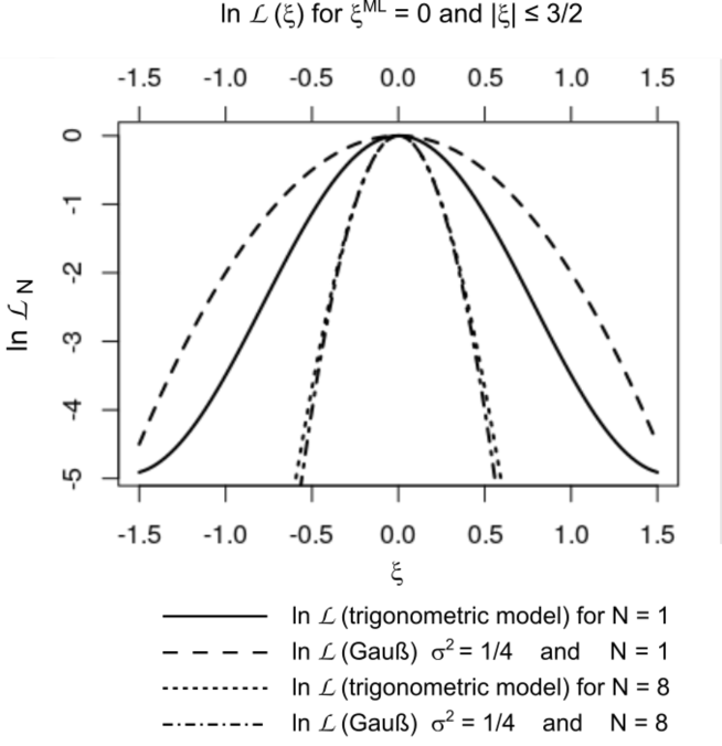
Figure 2: The graph compares a logarithmic likelihood function of the trigonometric model with form invariance to that of a Gaussian (i.e. a parabola) for $N=1\,$ and $N=8\,$. The former is taken from Eq. (83), the latter from Eq. (27) with $\sigma^{2}=F^{-1}=1\,.$ The curvature of the Gaussian agrees with the curvature of the likelihood function at their maxima. This figure also illustrates the reflection symmetry of the trigonometric model with respect to $\xi=0\,.$ With increasing $N$ the likelihood functions are ever more concentrated around their maximum value. This is illustrated by the comparison between $N=1$ and $N=8\,.$

The functional $H(\xi^{\rm ML}|\xi)$ exists and has the property (28) because the integral in (83) exists although the function $\cos^{2}s^{\prime}$ with, e.g.,

$$s^{\prime}\,=\,s-\xi$$ (84)

will vanish at an isolated point $s_{0}^{\prime}$ and $\ln\cos^{2}s_{0}^{\prime}$ will diverge. Appendix H shows that the integral over an $\epsilon$-interval that includes $s_{0}^{\prime}$, does exist. Here, $\epsilon$ may be arbitrarily small. The value of this integral is not proportional to $\epsilon\,;$ instead it is proportional to $\epsilon\ln\epsilon\,.$ Although this is not as small as $\epsilon\,,$ it approaches zero when $\epsilon\to 0\,.$ Thus the logarithmic likelihood $\ln{\cal L}_{N}$ of Eq. (83) exists even if the integration runs over a point where $\ln\cos^{2}$ diverges.

Applying the substitution (84) to the integrand in (83) one obtains

$$\ln{\cal L}_{N}\, = \,N{\cal N}\int_{-\pi/2}^{\pi/2}{\rm d}s^{\prime}\,\cos^{2}s^{\prime}\ln\frac{\cos^{2}(s^{\prime}-\xi+\xi^{\rm ML})}{\cos^{2}s^{\prime}}$$ (85)

$$= \,NH(0|\xi-\xi^{\rm ML})\,.$$

The substitution does not require a shift of the limits of integration because the integrand is periodic with a period of length $\pi$ and the integration covers one period. Thus the functional $H(\xi^{\rm ML}|\xi)$ for the translationally invariant trigonometric model has the property (28) which was found earlier for models defined on the entire real axis.

The fact that ${\cal L}_{N}$ equals $N$ times $H(0|-\alpha)$ shows that Eq. (34) holds here, too: The posterior distribution from $N$ events of the trigonometric model is proportional to the $N$-th power of the posterior from one event.

5 The Gaussian Approximation to the Trigonometric Model with Translational Invariance

The present section establishes the criterion for the validity of the Gaussian approximation to the likelihood function of the trigonometric model with translational invariance. In analogy to the procedure in Sect. 3 we expand $H(\xi^{\rm ML}|\xi)$ into a Taylor series with respect to $\xi$ at $\xi^{\rm ML}\,.$ Again the zero-th order of this expansion vanishes by the definition of $H$ in Eq. (24). Again the likelihood function is related to $H$ via Eq. (25). Using the abbreviation (120), introduced in appendix F, we obtain

$$H(0|\xi-\xi^{\rm ML})\,=\,H(\xi^{\rm ML}-\xi|0)\,.$$ (86)

Appendix F furthermore shows that the expression (86) is mirror symmetric with respect to $\xi^{\rm ML}-\xi=0\,,$ i.e.

$$H(0|\xi-\xi^{\rm ML})\,=\,H(0|\xi^{\rm ML}-\xi)\,.$$ (87)

Therefore all odd derivatives of $H(0|\xi^{\rm ML}-\xi)$ vanish at $\xi^{\rm ML}-\xi=0\,,$ thus

$$\left.\frac{\partial^{2\nu+1}}{\partial\xi^{2\nu+1}}\,H(0|\\ xi^{\rm ML}-\xi)\right|_{\xi=\xi^{\rm ML}}\,=\,0\,,\quad\quad\quad\nu=\,0,1,2,\dots\,.$$ (88)

By consequence, the remainder of the present expansion is not of the third order as it is in Sect. 3.1; it rather is of the fourth order.

All even derivatives $\frac{\partial^{2\nu}}{\partial\alpha^{2\nu}}H(0|\alpha)$ exist. Therefore in the present context the Taylor expansion (36) becomes

$$H(\xi^{\rm ML}|\xi)\,=\,-\frac{(\xi^{\rm ML}-\xi)^{2}}{2}F\,+\,\frac{(\xi^{\rm ML}-\xi)^{4}}{4!}\left.\frac{\partial^{4}}{\partial\xi^{4}}H(\xi^{\rm ML}|\xi)\right|_{\xi=\xi^{\rm ML}+(\xi^{\rm ML}-\xi)\Theta}\,.$$ (89)

In analogy to Sect. 3.1 the Gaussian approximation is considered valid when the term of fourth order is negligible as compared to the term of second order for all $\xi-\xi^{\rm ML}$ in the interval (38). See FIG. 2. For these values of $\xi$ we have to find the maximum of the absolute value of the fourth derivative in Eq. (89). We call it $|H^{(4)}|_{\rm max}\,.$ In analogy to Eq. (42) the Gaussian approximation is accepted when

$$\frac{1}{2}\big{(}\frac{3\sigma}{\sqrt{N}}\big{)}^{2}F\,\gg\,\frac{1}{24}\big{(}\frac{3\sigma}{\sqrt{N}}\big{)}^{4}|H^{(4)}|_{\rm max}$$ (90)

or

$$1\,\gg\,\frac{3}{4}\frac{\sigma^{2}}{N}\frac{|H^{(4)}|_{\rm max}}{F}\,.$$ (91)

As in Eq. (39) the Fisher information $F$ equals $\sigma^{-2}$ and we obtain the condition

$$1\,\gg\,\frac{3|H^{(4)}|_{\rm max}}{4NF^{2}}\,.$$ (92)

In appendix F the value of $|H^{(4)}|_{\rm max}$ is found to be

$$|H^{(4)}|_{\rm max}\,=\,16\,.$$ (93)

The value of the Fisher information $F$ is given by Eq. (81). Whence, the condition (92) for the Gaussian approximation becomes

$$1\,\gg\,\frac{3}{4N}\,.$$ (94)

We consider it to be fulfilled if

$$0.1\,\geq\,\frac{3}{4N}$$ (95)

or

$$N\,\geq\,8\,.$$ (96)

Thus the condition (96) for the Gaussian approximation to the binomial model is much more easily fulfilled than the corresponding condition (44) for the chi-squared model. The reason is: In Sect. 3.1 the remainder was of third order; in the present case it is of fourth order.

The step from (94) to (95) is due to the common idea that a given positive $x$ be large against $y>0$ when $x$ is one order of magnitude larger than $y\,.$ This idea is commonly used for approximations in mathematics [8] and physics [10]. If a higher accuracy is required, this rule can easily be adapted.

In Chap. 12 of [25] a version of Item Response Theory is presented which makes use of the trigonometric IRF (60). In that context a (simulated) competence test was discussed which asked $20$ questions. From the present result (96) follows that the estimated person-parameters have a Gaussian posterior distribution.

In Sect. 3.2 as well as in the present section the condition for the Gaussian approximation is independent of the value of $\xi^{\rm ML}\,.$ In the case of the binomial model, this means that the Gaussian approximation is valid even for uniform or close to uniform patterns of answers.

6 Conclusions

The present text presents a criterion for the validity of the Gaussian approximation to the likelihood function of a statistical model $p$ when $N$ observations $\mathbb{x}=(x_{1},\dots,x_{N})$ have been collected.

We require that a statistical model possesses a symmetry between the observed quantity $x$ and the parameter $\xi\,.$ This symmetry is defined in terms of a Lie group. It has been called form invariance. It allows to formally specify the prior distribution — required by Bayes but not specified by him. The model $p$ can then be parameterised such that it depends on the difference between the observed quantity $x$ and the parameter $\xi$ which conditions the observations. The model $p(x-\xi)$ remains invariant when both quantities are shifted by the same amount. We call this property translational form invariance. Then the likelihood function ${\cal L}_{N}(\xi)$ is shown to depend on the difference $\xi^{\rm ML}-\xi$ between the maximum likelihood estimator $\xi^{\rm ML}$ and the parameter $\xi\,.$ This means that the Bayesian posterior distribution, too, depends on $\xi^{\rm ML}-\xi\,.$ One can even shift the scale of $\xi$ such that the ML estimator is found at $\xi^{\rm ML}=0\,.$

A total of $N$ observations conditioned by one and the same parameter $\xi$ is generally expected to lead to a Gaussian likelihood function for sufficiently large $N\,.$ The question of how large $N$ must be, in order to justify the Gaussian approximation, is answered in Sects. 3 and 5 for two quite different examples. The basic idea is, that a valid Gaussian approximation to the posterior distribution means that the error assigned to the parameter $\xi$ equals $\sigma=(NF)^{-1/2}$ within the interval $|\xi^{\rm ML}-\xi|<3\sigma\,.$ Here, $F$ is the Fisher information yielded by the model $p\,.$ The probability for $\xi$ to lie outside this $3\sigma$-interval is neglected. A stricter condition for the Gaussian approximation would be achieved by requiring an interval larger than $3\sigma$ for its validity.

The example of Sect. 3 is a version of the chi-squared model with two degrees of freeedom. This distribution, as well as its posterior, has a considerable skewness. In this case one needs $N=160$ observations for the Gaussian approximation to be acceptable. The large number of required observations is due to the skewness.

The example of Sect. 5 is the trigonometric model, a specific form of the binomial model based on form invariance. It strongly differs from the chi-squared model since the observations are not taken from a continuum of real numbers but rather from the alternative of $0$ or $1\,.$ The likelihood function turns out to exhibit a mirror symmetry — as the Gaussian exhibits, too. This helps to approach the Gaussian distribution. We find: For $N\geq 8$ the posterior of the trigonometric model can be considered as Gaussian. This holds for every value of the ML estimator. It is a favorable result for the application of the binomial model to competence tests such as the PISA studies [46].

In general, we see a practical interest in our results since the normal distribution is the basis of parametric methods in applied statistics, widely used in many areas (education, medicine, science, etc.). To know whether the normal distribution is applicable or not, is of interest for practitioners in these fields.

Appendix A Comparing Two Distributions

We show that for any two normalised distributions $p$ and $q$ the unequality

$$\sum_{l}\,p_{l}\ln\frac{q_{l}}{p_{l}}\,\leq\,0$$ (97)

holds provided that $p$ and $q$ are labelled by the entire numbers $l$ and are normalised according to

$$\sum_{l}\,q_{l}\, = \,1\,,$$

$$\sum_{l}\,p_{l}\, = \,1\,.$$ (98)

The l.h.s. of (97) attains its maximum value of zero when and only when $p_{l}$ and $q_{l}$ agree for every $l\,.$

The unequality (97) is a consequence of the unequality

$$\ln s\,\leq\,s-1\,\quad\quad\quad{\rm for}\,\,\,s>0\,.$$ (99)

The linear function $s-1$ is tangent to the function $\ln s\,.$ The common point lies at $s=1\,,$ where both functions have the value of $1\,.$ Setting $s=q_{l}/p_{l}$ the unequality entails

$$\ln\frac{q_{l}}{p_{l}}\,\leq\,\frac{q_{l}}{p_{l}}-1$$ (100)

or

$$p_{l}\ln\frac{q_{l}}{p_{l}}\,\leq\,q_{l}-p_{l}$$ (101)

for every $l\,.$ The quantity on the l.h.s. has also been introduced by Campbell in Sect. 1 of Chap. 5 of [9]. Summing (101) over $l$ yields the unequality (97). When the distributions $p$ and $q$ agree whith each other, the l.h.s. of (97) vanishes. Then and only then the expression assumes its maximum value.

One can interprete $p_{l}$ as the probability $p(x_{l}-\xi^{\rm ML})\frac{\Delta x}{N}$ contained in a bin centered at the value $x_{l}$ of the real variable $x$ and having the width $\frac{\Delta x}{N}\,.$ Here, $p$ shall be a normalised probability density. Similarly one can interprete $q_{l}$ as the probability $p(x_{l}-\xi)\frac{\Delta x}{N}\,.$ In the limit of $\frac{\Delta x}{N}\to 0$ the unequality (97) then yields the unequality

$$\frac{1}{N}\int_{{\rm domain}\,x}{\rm d}x\,p(x-\xi^{\rm ML})\ln\frac{p(x-\xi)}{p(x-\xi^{\rm ML})}\,\leq\,0.$$ (102)

or

$$\int_{{\rm domain}\,x}{\rm d}x\,p(x-\xi^{\rm ML})\ln p(x-\xi)\,\leq\,\int_{{\rm domain}\,x}p(x-\xi^{\rm ML})\ln p(x-\xi^{\rm ML})\,.$$ (103)

Appendix B The ML Estimator of the Chi-Squared Model

The ML estimator of the chi-squared model (45) is calculated.

Up to an additive constant (independent of $\xi$) the logarithmic likelihood function is given by

$$\ln{\cal L}_{N}(\xi)\,=\,{\rm const}+[x-\xi-\exp(x-\xi)]\,.$$ (104)

The ML estimator $\xi^{\rm ML}$ solves the ML equation

$$0\, = \,\frac{\rm d}{{\rm d}\xi}\ln{\cal L}_{N}(\xi)$$ (105)

$$= \,-1+\exp(x-\xi)$$

The solution is

$$\xi^{\rm ML}\,=\,x\,.$$ (106)

Appendix C Two Versions of the Fisher Information

It shall be shown that the two lines of Eq. (30) agree with each other. Let us start from the second line which we write as

$$\frac{\partial^{2}}{\partial\xi^{2}}p(\mathbb{x}|\xi)\,=\,\left.\frac{\partial^{2}}{\partial\xi^{\prime 2}}\int_{-\infty}^{\infty}{\rm d}x\,p(x|\xi)\ln p(x|\xi^{\prime})\right|_{\xi^{\prime}=\xi}\,.$$ (107)

This expression can be rewritten

$$F(\xi) = \,-\left.\frac{\partial}{\partial\xi^{\prime}}\int{\rm d}x\,p(x|\xi)\,\frac{\frac{\partial}{\partial\xi^{\prime}}p(x|\xi^{\prime})}{p(x|\xi^{\prime})}\right|_{\xi^{\prime}=\xi}$$ (108)

$$= \,-\int{\rm d}x\,p(x|\xi)\left[\frac{\frac{\partial^{2}}{\partial\xi^{\prime 2}}p(x|\xi^{\prime})}{p(x|\xi^{\prime})}-\left(\frac{\frac{\partial}{\partial\xi^{\prime}}p(x|\xi^{\prime})}{p(x|\xi^{\prime})}\right)^{2}\right]_{\xi^{\prime}=\xi}$$

$$= \,-\int{\rm d}x\,\left[\frac{\partial^{2}}{\partial\xi^{2}}p(x|\xi)-p(x|\xi)\left(\frac{\partial}{\partial\xi}\ln p(x|\xi)\right)^{2}\right]$$

$$= -\frac{\partial^{2}}{\partial\xi^{2}}\int_{-\infty}^{\infty}{\rm d}x\,p(x|\xi)\,+\,\int_{-\infty}^{\infty}{\rm d}x\,p(x|\xi)\left(\frac{\partial}{\partial\xi}\ln p(x|\xi)\right)^{2}\,.$$

The first one of the two integrals in the last line vanishes since $p$ is normalised to unity for every $\xi\,.$ The second integral in the last line corresponds to the first line of Eq. (30).

Appendix D The Chi-Squared Model

Each of the quantities $x_{k}\,,$ where $k=1,2\,,$ shall have the Gaussian distribution

$$w(x_{k}|\sigma)\,=\,(2\pi\sigma^{2})^{-1/2}\exp\Big{(}-\frac{x_{k}^{2}}{2\sigma^{2}}\Big{)}\,,\quad\quad-\infty<x_{k}<\infty\,,$$ (109)

with one and the same root mean square value $\sigma\,.$ The chi-squared model $\chi_{2}^{\rm sq}(T|\sigma)$ with two degrees of freedom is the distribution of the quantity

$$T\,=\,x_{1}^{2}+x_{2}^{2}\,.$$ (110)

It is given by

$$\chi_{2}^{\rm sq}(T|\sigma)\,=\,\frac{1}{2\sigma^{2}\Gamma(1)}\exp\Big{(}-\frac{T}{2\sigma^{2}}\Big{)}\,,\quad\quad 0<T,\tau<\infty\,,$$ (111)

see e.g. Eq. (4.34) of Ref. [25]. This distribution is normalised to unity. The transformations

$$z\, = \,\ln T\,,$$

$$\zeta\, = \,\ln(2\sigma^{2})$$ (112)

lead to

$$\tilde{\chi}_{2}^{\rm sq}(z|\zeta)\, = \,\frac{{\rm d}T}{{\rm d}z}\,\chi_{2}^{\rm sq}(T|\sigma)$$ (113)

$$= \,T\,\chi_{2}^{\rm sq}(T|\sigma)\,,$$

where $T$ and $\sigma$ must be expressed by $z$ and $\zeta\,.$ This gives

$$\tilde{\chi}_{2}^{\rm sq}(z|\zeta)\,=\,\,\exp\Big{(}z-\zeta-e^{z-\zeta}\Big{)}$$ (114)

which corresponds to Eq. (45).

Appendix E Derivatives of the Functional $H$ for the chi-Squared Distribution

The integral in the first line of Eq. (50) yields $\Gamma(2)\,.$ It is a special case of the formula

$$\Gamma(z)\,=\,\int_{-\infty}^{\infty}{\rm d}t\,\exp(zt-e^{t})$$ (115)

given in Sect. 8.312, no. 10 of Ref. [22]. The value of the Gamma function required in Eq. (50) is

$$\Gamma(2)\,=\,2\,.$$ (116)

Appendix F The Functional $H$ for the Trigonometric Model with Translational Invariance

The functional $H(\xi^{\rm ML}|\xi)$ for the trigonometric model model (75) is given by Eq. (83) to be

$$H(\xi^{\rm ML}|\xi)\,=\,{\cal N}\int_{-\pi/2}^{\pi/2}{\rm d}s\,\cos^{2}(s-\xi^{\rm ML})\ln\frac{\cos^{2}(s-\xi)}{\cos^{2}(s-\xi^{\rm ML})}\,.$$ (117)

The substitution

$$s^{\prime}\,=\,s-\xi^{\rm ML}$$ (118)

yields

$$H(\xi^{\rm ML}|\xi)\, = \,{\cal N}\int_{-\pi/2+\xi^{\rm ML}}^{\pi/2+\xi^{\rm ML}}{\rm d}s^{\prime}\,\cos^{2}s^{\prime}\ln\frac{\cos^{2}(s^{\prime}-\xi+\xi^{\rm ML})}{\cos^{2}s^{\prime}}$$ (119)

$$= \,{\cal N}\int_{-\pi/2}^{\pi/2}{\rm d}s^{\prime}\,\cos^{2}s^{\prime}\ln\frac{\cos^{2}(s^{\prime}-\xi+\xi^{\rm ML})}{\cos^{2}s^{\prime}}$$

$$= \,H(0|\xi-\xi^{\rm ML})\,.$$

Here, the second line is obtained from the first one because the integrand is periodic with a period of $\pi\,,$ hence, the shift of the limits of integration is immaterial. With the abbreviation

$$\alpha=\xi^{\rm ML}-\xi$$ (120)

this reads

$$H(\xi^{\rm ML}|\xi)\, = \,H(0|-\alpha)$$ (121)

$$= \,{\cal N}\int_{-\pi/2}^{\pi/2}{\rm d}s\,\cos^{2}s\ln\frac{\cos^{2}(s+\alpha)}{\cos^{2}s}\,.$$

Substituting

$$s^{\prime}\,=\,-s$$ (122)

in the integral (121) one obtains

$$H(0|-\alpha)\, = \,-{\cal N}\int_{\pi/2}^{-\pi/2}{\rm d}s^{\prime}\,\cos^{2}s^{\prime}\ln\frac{\cos^{2}(-s^{\prime}+\alpha)}{\cos^{2}s^{\prime}}$$ (123)

$$= \,{\cal N}\int_{-\pi/2}^{\pi/2}{\rm d}s^{\prime}\,\cos^{2}s^{\prime}\ln\frac{\cos^{2}(s^{\prime}-\alpha)}{\cos^{2}s^{\prime}}$$

$$= \,H(0|\alpha)\,.$$

Although $\cos(s-\alpha)$ vanishes at a point within the domain of integration, the integral (123) exists and can be obtained as if the integrand were simply undefined at this isolated point, see appendix H.

Comparing (121) with (123) shows that $H(0|-\alpha)$ is a mirror-symmetrical function of the difference $\alpha\,.$ By consequence, all odd derivatives vanish at $\alpha=0\,,$

$$\left.\frac{\partial^{2\nu+1}}{\partial\alpha^{2\nu+1}}H(0|-\alpha)\right|_{\alpha=0}\,=\,0\,,\quad\quad\quad\nu=0,1,2,\dots\,.$$ (124)

We calculate the derivatives with respect to $\alpha\,.$ The first derivative is the basis of all higher ones. It must be rewritten in order to see that all derivatives exist. Starting from Eq. (123) we find

$$\frac{\partial}{\partial\alpha}H(0|-\alpha)\, = \,{\cal N}\frac{\partial}{\partial\alpha}\int_{-\pi/2}^{\pi/2}{\rm d}s\,\left[\cos^{2}s\ln\cos^{2}(s-\alpha)\,-\cos^{2}s\ln\cos^{2}s\right]$$ (125)

$$= \,{\cal N}\frac{\partial}{\partial\alpha}\int_{-\pi/2}^{\pi/2}{\rm d}s\,\cos^{2}s\ln\cos^{2}(s-\alpha)\,.$$

By use of the substitution

$$s^{\prime}\,=\,s-\alpha$$ (126)

one obtains from the integral (125)

$$\frac{\partial}{\partial\alpha}H(0|-\alpha)\, = \,{\cal N}\frac{\partial}{\partial\alpha}\int_{-\pi/2}^{\pi/2}{\rm d}s\,\cos^{2}(s+\alpha)\ln\cos^{2}s$$ (127)

$$= \,2{\cal N}\frac{\partial}{\partial\alpha}\int_{-\pi/2}^{\pi/2}{\rm d}s\,\cos^{2}(s+\alpha)\ln\cos s\,.$$

We express $\cos(s+\alpha)$ by the sum

$$\cos(s+\alpha)\,=\,\cos s\cos\alpha-\sin s\sin\alpha$$ (128)

and obtain

$$\frac{\partial}{\partial\alpha}H(0|-\alpha)\,=\,2{\cal N}\frac{\partial}{\partial\alpha}\int_{-\pi/2}^{\pi/2}{\rm d}s\,\left[\cos s\cos\alpha-\sin s\sin\alpha\right]^{2}\ln\cos s\,.$$ (129)

The square $\left[\dots\right]^{2}$ of a binomial expression displays two squares and a mixed term. Here, the mixed term, as a function of $s\,,$ is antisymmetric with respect to $s=0\,.$ Therefore the integral over the mixed term vanishes and we obtain

$$\frac{\partial}{\partial\alpha}H(0|-\alpha)\,=\,2{\cal N}\frac{\partial}{\partial\alpha}\int_{-\pi/2}^{\pi/2}{\rm d}s\,\left[\cos^{2}s\cos^{2}\alpha+\sin^{2}s\sin^{2}\alpha\right]\ln\cos s\,.$$ (130)

This integrand, as a function of $s\,,$ is symmetric with respect to $s=0\,.$ Therefore we have

$$\frac{\partial}{\partial\alpha}H(0|-\alpha)\, = \,4{\cal N}\frac{\partial}{\partial\alpha}\cos^{2}\alpha\int_{0}^{\pi/2}{\rm d}s\,\cos^{2}s\ln\cos s+\,4{\cal N}\frac{\partial}{\partial\alpha}\sin^{2}\alpha\int_{0}^{\pi/2}{\rm d}s\,\sin^{2}s\ln\cos s$$ (131)

$$= \,8{\cal N}\cos\alpha\sin\alpha\left[-\int_{0}^{\pi/2}{\rm d}s\,\cos^{2}s\ln\cos s+\int_{0}^{\pi/2}{\rm d}s\,\sin^{2}s\ln\cos s\right]\,.$$

Let us introduce the integrals

$$I_{0}\,=\,\int_{0}^{\pi/2}{\rm d}s\,\ln\cos s$$ (132)

and

$$I_{2}\,=\,\int_{0}^{\pi/2}{\rm d}s\,\sin^{2}s\ln\cos s\,.$$ (133)

They allow to write Eq. (131) as

$$\frac{\partial}{\partial\alpha}H(0|-\alpha)\,=\,8{\cal N}[-I_{0}+2I_{2}]\cos\alpha\sin\alpha$$ (134)

which gives

$$\frac{\partial}{\partial\alpha}H(0|-\alpha)\,=\,-4{\cal N}[I_{0}-2I_{2}]\sin(2\alpha)$$ (135)

by help of the identity

$$\sin(2\alpha)\,=\,2\cos\alpha\sin\alpha\,.$$ (136)

The derivative (135) vanishes at $\alpha=0\,,$ as expected from Eq. (124).

The values of the integrals (132) and (133) can be taken from the table of integrals [22]. According to the entries 4.387 no. 3 and 8.366 no. 1,2 of [22], the integral (132) has the value

$$I_{0}\,=\,-\frac{\pi}{2}\ln 2$$ (137)

while the entries 4.387 no. 8 and 8.365 no. 1 as well as 8.366 no.1 yield

$$I_{2}\,=\,-\frac{\pi}{8}[2\ln 2+1]\,.$$ (138)

These two values lead to

$$I_{0}-2I_{2}\,=\,\frac{\pi}{4}\,.$$ (139)

Together with the value of ${\cal N}$ in Eq. (77) the derivative (135) becomes

$$\frac{\partial}{\partial\alpha}H(0|-\alpha)\,=\,-2\sin(2\alpha)\,.$$ (140)

Therefore the second derivative of $H(0|-\alpha)$ becomes

$$\frac{\partial^{2}}{\partial\alpha^{2}}H(0|-\alpha)\,=\,-4\cos(2\alpha)$$ (141)

and the fourth derivative becomes

$$\frac{\partial^{4}}{\partial\alpha^{4}}H(0|-\alpha)\,=\,16\cos(2\alpha)\,.$$ (142)

The maximum of the absolute value of the fourth derivative is found at $\alpha=0$ which means

$$|H^{(4)}|_{\rm max}\,=\,16\,.$$ (143)

Note that the second derivative in Eq. (141) for $\alpha=0$ gives the value

$$\left.\frac{\partial^{2}}{\partial\alpha^{2}}H(0|\alpha)\right|_{\alpha=0}\,=\,-4$$ (144)

which is, up to its sign, the Fisher information (81) of the trigonometric model with translational invariance.

Appendix G The Normalisation of the Trigonometric Model with Translational Invariance

By partial integration of the $\cos^{2}$-function one finds

$$\int_{-\pi/2}^{\pi/2}{\rm d}s\,\cos^{2}s\,=\,\big{[}\sin s\cos s\big{]}_{-\pi/2}^{\pi/2}\,+\,\int_{-\pi/2}^{\pi/2}{\rm d}s\,\sin^{2}s\,.$$ (145)

This leads to

$$\int_{-\pi/2}^{\pi/2}{\rm d}s\,\cos^{2}s\,=\,\int_{-\pi/2}^{\pi/2}{\rm d}s\,(1-\cos^{2}s)$$ (146)

or

$$2\int_{-\pi/2}^{\pi/2}{\rm d}s\,\cos^{2}s\,=\,\pi$$ (147)

which proves Eq. (77).

Appendix H Integrating over a Logarithmic Divergence

In the $\epsilon$-interval

$$-\epsilon\,<\,s^{\prime}-s_{0}^{\prime}\,<\,\epsilon\,,\quad\quad\epsilon>0\,,$$ (148)

around the point $s_{0}^{\prime}\,,$ where $\cos^{2}$ vanishes, the $\cos^{2}$-function behaves as

$$\cos^{2}s^{\prime}\,=\,c(s^{\prime}-s_{0}^{\prime})^{2}$$ (149)

since the $\cos^{2}$-function does not become negative and $\epsilon$ can be chosen arbitrarily small. Here, $c$ is a positive number. We show that the integral over the $\epsilon$-interval

$$\int_{s_{0}^{\prime}-\epsilon}^{s_{0}^{\prime}+\epsilon}{\rm d}s^{\prime}\,\ln\cos^{2}s^{\prime}\,=\,2\epsilon\ln c\,+\,\int_{s_{0}^{\prime}-\epsilon}^{s_{0}^{\prime}+\epsilon}{\rm d}s^{\prime}\,\ln(s^{\prime}-s_{0}^{\prime})^{2}$$ (150)

exists.

For this we rewrite

$$\int_{s_{0}^{\prime}-\epsilon}^{s_{0}^{\prime}+\epsilon}{\rm d}s^{\prime}\,\ln(s^{\prime}-s_{0}^{\prime})^{2} = \,\int_{s_{0}^{\prime}-\epsilon}^{s_{0}^{\prime}}{\rm d}s^{\prime}\,\ln(s^{\prime}-s_{0}^{\prime})^{2}\,+\,\int_{s_{0}^{\prime}}^{s_{0}^{\prime}+\epsilon}{\rm d}s^{\prime}\,\ln(s^{\prime}-s_{0}^{\prime})^{2}$$

$$= \,2\int_{s_{0}^{\prime}-\epsilon}^{s_{0}^{\prime}}{\rm d}s^{\prime}\,\ln(s_{0}^{\prime}-s^{\prime})\,+\,2\int_{s_{0}^{\prime}}^{s_{0}^{\prime}+\epsilon}{\rm d}s^{\prime}\,\ln(s^{\prime}-s_{0}^{\prime})$$

so that the arguments of the logarithms are non-negative. In the first integral of the second line we substitute

$$s_{0}^{\prime}-s^{\prime}\,=\,x$$ (152)

and obtain

$$2\int_{s_{0}^{\prime}-\epsilon}^{s_{0}^{\prime}}{\rm d}s^{\prime}\,\ln(s_{0}^{\prime}-s^{\prime})\, = \,-2\int_{\epsilon}^{0}{\rm d}x\,\ln x$$ (153)

$$= \,2\int_{0}^{\epsilon}{\rm d}x\,\ln x$$

$$= \,2\big{[}x\ln x-1\big{]}_{x=0}^{x=\epsilon}$$

$$= \,2\epsilon\ln\epsilon\,.$$

In a similar way one finds the same result for the second integral on the second line of (LABEL:H.4). Thus Eq. (150) yields

$$\int_{s_{0}^{\prime}-\epsilon}^{s_{0}^{\prime}+\epsilon}{\rm d}s^{\prime}\,\ln\cos^{2}s_{0}^{\prime}\,=\,2\epsilon\ln c\,+\,4\epsilon\ln\epsilon\,,$$ (154)

and this contributes a negligible amount to the expression (82) when $\epsilon$ is small. Thus $\ln{\cal L}_{N}$ and the functional $H(\xi^{\rm ML}|\xi)$ exist.

Appendix I The Likelihood Function of a Gaussian Model

The $N$-fold Gaussian model

$$G_{N}(\mathbb{x}|\xi)\,=\,(2\pi\sigma^{2})^{-N/2}\prod_{k=1}^{N}\,\exp\left(-\frac{(x_{k}-\xi)^{2}}{2\sigma^{2}}\right)$$ (155)

is given in Eq. (7). We write it as

$$G_{N}(\mathbb{x}|\xi)\, = \,(2\pi\sigma^{2})^{-N/2}\exp\left(-\frac{1}{2\sigma^{2}}\sum_{k=1}^{N}\,(x_{k}^{2}-2x_{k}\xi+\xi^{2})\right)$$ (156)

$$= \,(2\pi\sigma^{2})^{-N/2}\exp\left(-\frac{1}{2\sigma^{2}}\sum_{k=1}^{N}\,(<x^{2}>-2<x>\xi+\xi^{2})\right)$$

by introducing the averages

$$<x^{2}>\, = \,\frac{1}{N}\sum_{k=1}^{N}\,x_{k}^{2}\,,$$

$$<x>\, = \,\frac{1}{N}\sum_{k=1}^{N}\,x_{k}\,.$$ (157)

It is not difficult to factorise this according to

$$G_{N}(\mathbb{x}|\xi)\,=\,(2\pi\sigma^{2})^{-N/2}\left(\exp(-\frac{N}{2\sigma^{2}}(<x^{2}>-<x>^{2})\right)\exp\left(-\frac{N}{2\sigma^{2}}(<x>-\xi)^{2}\right)\,.$$ (158)

The posterior distribution $G_{N}(\xi|\mathbb{x})$ is given by the factor that depends on $\xi\,,$ i.e.

$$G_{N}(\xi|\mathbb{x})\,\propto\,\exp\left(-\frac{N}{2\sigma^{2}}(<x>-\xi)^{2}\right)$$ (159)

in agreement with Eq. (8). The maximum of the likelihood function occurs at

$$\xi^{\rm ML}\,=\,<x>\,.$$ (160)

Appendix J The Fisher Information of the Binomial Model

The Fisher information of the model binomial model (59) shall be independent of $\xi\,.$ This means that the expression

$$F(\xi)\, = \,\sum_{x=0}^{1}\,q(x|\xi)\left[\frac{\partial}{\partial\xi}\ln q(x|\xi)\right]^{2}$$ (161)

$$= \,[1-R]\left[\frac{R^{\prime}}{1-R}\right]^{2}\,+\,R\left[\frac{R^{\prime}}{R}\right]^{2}$$

$$= \,\frac{[R^{\prime}]^{2}}{1-R}\,+\,\frac{[R^{\prime}]^{2}}{R}$$

$$= \,\frac{[R^{\prime}]^{2}}{R[1-R]}$$

be independent of $\xi\,.$ Here, $R^{\prime}$ is the derivative of $R(\xi)\,.$ Thus the numerator of (161) should be proportional to the denominator. This is reached when we set

$$R(\xi)\,=\,\cos^{2}\xi\,,\quad\quad\quad-\pi/2\leq\xi\leq\pi/2$$ (162)

and obtain

$$F(\xi)\,\equiv\,4\,.$$ (163)

References

- [1] J. Frank Adams. Lectures on Lie Groups. W.A. Benjamin, New York, 1969.
- [2] John Aldrich. R.A. Fisher and the Making of the Maximum Likelihood 1912–1922. Statistical Science, 12(3):172–176, 1997.
- [3] A. Aykac and C. Brumat, editors. New Methods in the Applications of Bayesian Methods, volume 1. North Holland, Amsterdam, 1977.
- [4] Thomas Bayes. An essay towards solving a problem in the doctrine of chances. Phil. Trans. Roy. Soc., 53:330–418, 1763. Reprinted in Biometrika 45, 293–315 (1958) and in ‘Studies in the History of Statistics and Probability’ E.S. Pearson and M.G. Kendall eds., C.Griffin and Co. Ltd., London 1970 and in ’Two papers by Bayes with commentaries’ W.E. Deming ed., Hafner Publishing Co., New York, 1963.
- [5] J.M. Bernardo, M.H. DeGroot, D.V. Lindley, and A.F.M Smith, editors. Bayesian Statistics 3. Proceedings of the third International Meeting held at Valencia on June 1–5, 1987, Oxford, 1988. Oxford University Press.
- [6] Andrew C. Berry. The accuracy of the Gaussian approximation to the sum of independent variables. Transactions of the American Mathematical Society, 49:122–136, 1941.
- [7] Theodor Bröcker and Tammo tom Dieck. Representations of Compact Lie Groups. Springer, New York, 1985.
- [8] I.N. Bronstein, K.A. Semendyayev, G. Musiol, and H. Muehlig. Handbook of Mathematics. Springer, New York, 4th edition, 2014.
- [9] L. Lore Campbell. Geometric ideas in minimum cross-entropy. In Jawaharlal Karmeshu, editor, Entropy measures, maximum entropy principle, and emerging applications, chapter 5, pages 103–114. Springer, Berlin, 2003.
- [10] K. Cummings, P.W. Laws, E.F. Redish, and P.J. Cooney. Understanding Physics. John Wiley and Sons, Hoboken N.J., 2004.
- [11] A.W.F. Edwards. Likelihood. Johns Hopkins University Press, Baltimore, 1992.
- [12] George A. Ferguson. Item selection by the constant process. Psychometrika, 7(1):19–29, 1942.
- [13] G.H. Fischer. On the existence and uniqueness of maximum-likelihood estimates in the Rasch model. Psychometrika, 46(1):59–77, 1981.
- [14] G.H. Fischer. Derivations of the Rasch model. In Rasch models: foundations, recent developments and applications, pages 15–38, New York, 1995. Workshop held at the University of Vienna, Feb. 25–27, 1993.
- [15] R.A. Fisher. An absolute criterion for fitting frequency curves. Messenger of Math., 41:155–160, 1912.
- [16] R.A. Fisher. On the mathematical foundations of theoretical statistics. Philos. Trans. Royal Soc. London Ser. A, 222:309–368, 1922.
- [17] R.A. Fisher. Theory of statistical information. Proc. Cambridge Philos. Soc., 22:700–725, 1925.
- [18] R.A. Fisher. Statistical Methods and Scientific Inference. Oliver and Boyd, Edinburgh, 2nd edition, 1959.
- [19] R.A. Fisher. Statistical Methods for Research Workers. Oliver and Boyd, Edinburgh, 1967. 13-th edition.
- [20] P.F. Fougère, editor. Maximum Entropy and Bayesian Methods, Dartmouth, 1989, Dordrecht, 1990. Kluwer.
- [21] Christoph Fuhrmann. Eine trigonometrische Parametrisierung von Kompetenzen. Zur Methodologie der probabilistischen Bildungsforschung. PhD thesis, Ruhr-Universität, Bochum, Germany, 2016. This dissertation is published by Springer VS, Wiesbaden (Germany), 2017.
- [22] I.S. Gradshteyn and I.M. Ryzhik. Table of Integrals, Series, and Products. Academic Press, New York, eighth edition, 2015. Edited by D. Zwillinger.
- [23] Louis Guttman. The basis of scalogram analysis, pages 60–90. Smith, Gloucester, Mass., 1973.
- [24] A. Haar. Der Maßbegriff in der Theorie der kontinuierlichen Gruppen. Ann. Math., 34:147–169, 1933.
- [25] H.L. Harney. Bayesian Inference. Parameter Estimation and Decisions. Springer, Heidelberg, 2016. Second edition.
- [26] J. Hartigan. Invariant prior distributions. Ann. Math. Statist., 35:836–845, 1964.
- [27] A. Hobson and B.K. Cheng. A comparison of the Shannon and Kullback information measures. J. of Statistical Physics, 7(4):301–310, 1973.
- [28] R.V. Hogg, E.A. Tanis, and D.L. Zimmermann. Probability and Statistical Inference. Pearson, Boston, 2015.
- [29] Shun ichi Amari. Differential Geometrical Methods in Statistics, volume 28 of Lecture Notes in Statistics. Springer, Heidelberg, 1985.
- [30] E.T. Jaynes. Prior probabilities. IEEE Transactions on Systems Science and Cybernetics, SSC-4(3):227–241, September 1968.
- [31] E.T. Jaynes and G.L. Bretthorst. Probability theory: The logic of Science. Cambridge Univ. Press, Cambridge, Mass., 2012.
- [32] H. Jeffreys. An invariant form of the prior probability in estimation problems. Proc. of the Roy. Soc., 186 A:453–461, 1946.
- [33] R.E. Kass. The Riemannian Structure of Model Spaces: A Geometrical Approach to Inference. PhD thesis, University of Chicago, 1980. See especially pages 94–95.
- [34] R.E. Kass. Data translated likelihood and Jeffreys’s rules. Biometrika, 77:107–114, 1990.
- [35] R.E. Kass and L. Wasserman. The selection of prior distributions by formal rules. J. Am. Statist. Assoc., 91:1343–1370, 1996.
- [36] Maurice Kendall and Alan Stuart. The Advanced Theory of Statistics, volume 2. Griffin, London, third edition, 1951. For the notion of sufficient statistic see p. 22.
- [37] Maurice Kendall and Alan Stuart. The Advanced Theory of Statistics. Griffin, London, fourth edition, 1976.
- [38] S. Kullback and R.A. Leibler. On information and sufficiency. Ann. Math. Statist., 22:79–86, 1951.
- [39] Pierre Simon de Laplace. Mémoire sur la probabilité des causes par les événements. Mém. de math. et phys. présentés à l’Acad. roy. des sci., 6:621–656, 1774. Reprinted in [40], vol. 8, pages 27–65. An English translation can be found in [57].
- [40] Pierre Simon de Laplace. Œuvres complètes de Laplace. Gauthier-Villars, Paris, 1886–1912. 14 volumes.
- [41] Paul F. Lazarsfeld. The logical and mathematical foundation of latent structure analysis. In Samuel A. Stouffer and Louis Guttman et al., editors, Measurement and Prediction. Smith, Gloucester, Mass., reprinted edition, 1973.
- [42] E.L. Lehmann and G. Casella. Theory of Point Estimation. Springer, New York, 1998.
- [43] Thurstone L.L.\̇lx@bibnewblockA method of scaling psychological and educational tests. Journal of Educational Psychology, 16(October):433–451, 1925.
- [44] Frederic M. Lord. Applications of item response theory to practical testing problems. Erlbaum, Hillsdale NJ, 1980.
- [45] J. Neyman and Elizabeth L. Scott. Consistent estimates based on partially consistent observations. Econometrica, 16:1–32, 1948.
- [46] OECD. PISA 2015. Technical report. www.oecd.org/pisa/sitedocument/PISA-2015-technical-report-final.pdf. This website was visited on November 3, 2018.
- [47] A. Papoulis and S.U. Pillai. Probability, random variables, and stochastic processes. McGraw-Hill, New York, 2002.
- [48] C. Radakrishna Rao. Differential metrics in probability spaces based on entropy and divergence measures. Technical Report Report No. AD-A160301, AFOSR-TR-85-0864, Air Force Office of Scientific Research, Bolling AFB, DC, 1985.
- [49] G. Rasch. An individual approach to item analysis. In P.F. Lazarsfeld and N.W. Henry, editors, Readings in mathematical social science, pages 89–108, Cambridge, 1966. Massachusetts Institute of Technology.
- [50] G. Rasch. An informal report on a theory of objectivity in comparisons. In L.J.Th. van der Kamp and C.A.J. Vlek, editors, Measurement theory. Proceedings of the NUFFIC international summer session in science at ‘Het Oude Hof‘. The Hague, July 14–28, 1966, pages 1–19, Leiden, 1967. University of Leiden.
- [51] G. Rasch. On specific objectivity: An attempt at formalising the request for generality and validity of scientific statements. Danish Yearbook of Philosophy, 14:58–94, 1977.
- [52] G. Rasch. Probabilistic Models for Some Intelligence and Attainment Tests. The University of Chicago Press, Chicago, 1980.
- [53] Georg Rasch. Probabilistic models for some intelligence and attainment tests with a foreword and afterword by Benjamin D. Wright. Danish Institute for Educational Research, 1960. expanded edition 1980 published by University of Chicago Press.
- [54] S.M. Ross. Introductory Statistics. Elsevier/AP, Amsterdam, 2017.
- [55] Jürgen Rost. Lehrbuch Testtheorie — Testkonstruktion. Hans Huber, Bern, second revised edition, 2004.
- [56] Aris Spanos. Revisiting the Neyman-Scott model: an inconsistent MLE or an ill-defined model?, 2013. arXiv:1301.6278v1 [stat.ME] 26 January 2013.
- [57] S.M. Stigler. Laplace’s 1774 memoir on inverse probability. Statist. Sci., 1:359–378, 1986.
- [58] S.M. Stigler. The epic story of maximum likelihood. Statistical Science, 22(4):598–620, 2007.
- [59] A. Zellner. An introduction to Bayesian inference in econometrics. Wiley, New York, 1996.
- [60] Arnold Zellner. Maximal Data Information Prior Distributions, chapter 12. Volume 1 of Aykac and Brumat [3], 1977.