Fully Convolutional Networks for Panoptic Segmentation

Abstract

In this paper, we present a conceptually simple, strong, and efficient framework for panoptic segmentation, called Panoptic FCN. Our approach aims to represent and predict foreground things and background stuff in a unified fully convolutional pipeline. In particular, Panoptic FCN encodes each object instance or stuff category into a specific kernel weight with the proposed kernel generator and produces the prediction by convolving the high-resolution feature directly. With this approach, instance-aware and semantically consistent properties for things and stuff can be respectively satisfied in a simple generate-kernel-then-segment workflow. Without extra boxes for localization or instance separation, the proposed approach outperforms previous box-based and -free models with high efficiency on COCO, Cityscapes, and Mapillary Vistas datasets with single scale input. Our code is made publicly available at https://github.com/Jia-Research-Lab/PanopticFCN.

1 Introduction

Panoptic segmentation, aiming to assign each pixel with a semantic label and unique identity, is regarded as a challenging task. In panoptic segmentation [19], countable and uncountable instances (i.e., things and stuff) are expected to be represented and resolved in a unified workflow. One main difficulty impeding unified representation comes from conflicting properties requested by things and stuff. Specifically, to distinguish among various identities, countable things usually rely on instance-aware features, which vary with objects. In contrast, uncountable stuff would prefer semantically consistent characters, which ensures consistent predictions for pixels with the same semantic meaning. An example is given in Fig. 1, where embedding of individuals should be diverse for inter-class variations, while characters of grass should be similar for intra-class consistency.

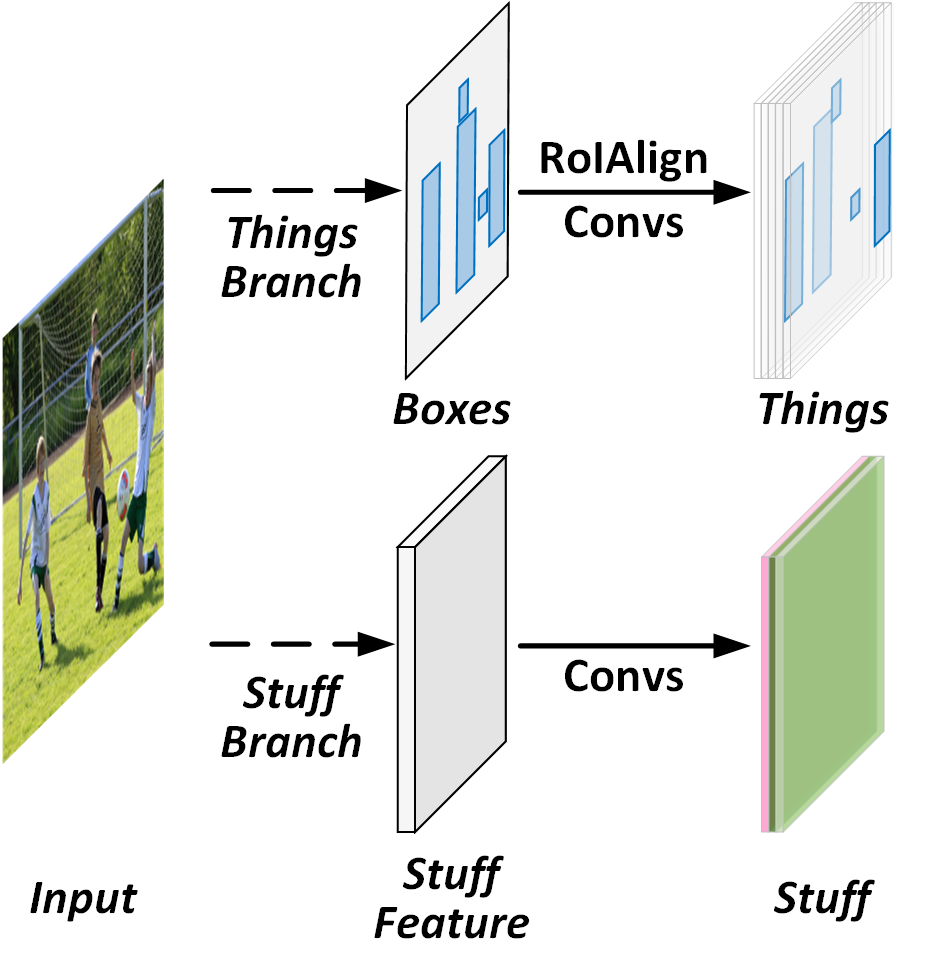
(a) Separate representation

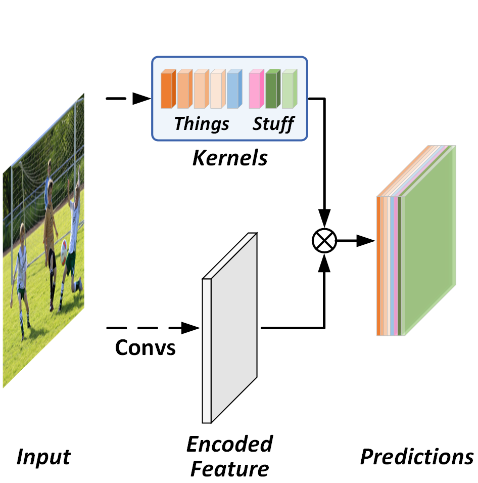
(b) Unified representation

Figure 1: Compared with traditional methods, which often utilize separate branches to handle things and stuff in 1(a), the proposed Panoptic FCN 1(b) represents things and stuff uniformly with generated kernels. Here, an example with box-based stream for things is given in 1(a). The shared backbone is omitted for concision.

For conflict at feature level, specific modules are usually tailored for things and stuff separately, as presented in Fig. 1(a). In particular, instance-aware demand of things is satisfied mainly from two streams, namely box-based [18, 50, 25] and box-free [51, 10, 6] methods. Meanwhile, the semantic-consistency of stuff is met in a pixel-by-pixel manner [33], where similar semantic features would bring identical predictions. A classic case is Panoptic FPN [18], which utilizes Mask R-CNN [12] and FCN [33] in separated branches to respectively classify things and stuff, similar to that of Fig. 1(a). Although attempt [51, 10, 6] has been made to predict things without boxes, extra predictions (e.g., affinities [10], and offsets [51]) together with post-process procedures are still needed to distinguish among instances, which slow down the whole system and hinder it from being fully convolutional. Consequently, a unified representation is required to bridge this gap.

In this paper, we propose a fully convolutional framework for unified representation, called Panoptic FCN. In particular, Panoptic FCN encodes each instance into a specific kernel and generates the prediction by convolutions directly. Thus, both things and stuff can be predicted together with a same resolution. In this way, instance-aware and semantically consistent properties for things and stuff can be respectively satisfied in a unified workflow, which is briefly illustrated in Fig. 1(b). To sum up, the key idea of Panoptic FCN is to represent and predict things and stuff uniformly with generated kernels in a fully convolutional pipeline.

To this end, kernel generator and feature encoder are respectively designed for kernel weights generation and shared feature encoding. Specifically, in kernel generator, we draw inspirations from point-based object detectors [20, 55] and utilize the position head to locate as well as classify foreground objects and background stuff by object centers and stuff regions, respectively. Then, we select kernel weights [17] with the same positions from the kernel head to represent corresponding instances. For the instance-awareness and semantic-consistency described above, a kernel-level operation, called kernel fusion, is further proposed, which merges kernel weights that are predicted to have the same identity or semantic category. With a naive feature encoder, which preserves the high-resolution feature with details, each prediction of things and stuff can be produced by convolving with generated kernels directly.

In general, the proposed method can be distinguished from two aspects. Firstly, different from previous work for things generation [12, 4, 45], which outputs dense predictions and then utilizes NMS for overlaps removal, the deigned framework generates instance-aware kernels and produces each specific instance directly. Moreover, compared with traditional FCN-based methods for stuff prediction [53, 3, 9], which select the most likely category in a pixel-by-pixel manner, our approach aggregates global context into semantically consistent kernels and presents results of existing semantic classes in a whole-instance manner.

The overall approach, named Panoptic FCN, can be easily instantiated for panoptic segmentation, which will be fully elaborated in Sec. 3. To demonstrate its superiority, we give extensive ablation studies in Sec. 4.2. Furthermore, experimental results are reported on COCO [29], Cityscapes [8], and Mapillary Vistas [35] datasets. Without bells-and-whistles, Panoptic FCN outperforms previous methods with efficiency, and respectively attains 44.3% PQ and 47.5% PQ on COCO val and test-dev set. Meanwhile, it surpasses all similar box-free methods by large margins and achieves leading performance on Cityscapes and Mapillary Vistas val set with 61.4% PQ and 36.9% PQ, respectively.

2 Related Work

Panoptic segmentation. Traditional approaches mainly conduct segmentation for things and stuff separately. The benchmark for panoptic segmentation [19] directly combines predictions of things and stuff from different models, causing heavy computational overhead. To solve this problem, methods have been proposed by dealing with things and stuff in one model but in separate branches, including Panoptic FPN [18], AUNet [25], and UPSNet [50]. From the view of instance representation, previous work mainly formats things and stuff from different perspectives. Foreground things are usually separated and represented with boxes [18, 52, 5, 24] or aggregated according to center offsets [51], while background stuff is often predicted with a parallel FCN [33] branch. Although methods of [23, 10] represent things and stuff uniformly, the inherent ambiguity cannot be resolved well merely with the pixel-level affinity, which yields the performance drop in complex scenarios. In contrast, the proposed Panoptic FCN represents things and stuff in a uniform and fully convolutional framework with decent performance and efficiency.

Instance segmentation. Instance segmentation aims to discriminate objects in the pixel level, which is a finer representation compared with detected boxes. For instance-awareness, previous works can be roughly divided into two streams, i.e., box-based methods and box-free approaches. Box-based methods usually utilize detected boxes to locate or separate objects [12, 32, 1, 21, 38]. Meanwhile, box-free approaches are designed to generate instances without assistance of object boxes [10, 4, 45, 46]. Recently, AdaptIS [40] and CondInst [42] are proposed to utilize point-proposal for instance segmentation. However, the instance aggregation or object-level removal is still needed for results. In this paper, we represent objects in a box-free pipeline, which generates the kernel for each object and produces results by convolving the detail-rich feature directly, with no need for object-level duplicates removal [15, 37].

Semantic segmentation. Semantic segmentation assigns each pixel with a semantic category, without considering diverse object identities. In recent years, rapid progress has been made on top of FCN [33]. Due to the semantically consistent property, several attempts have been made to capture contextual cues from wider perception fields [53, 2, 3] or establish pixel-wise relationship for long-range dependencies [54, 16, 41]. There is also work to design network architectures for semantic segmentation automatically [30, 26], which is beyond the scope of this paper. Our proposed Panoptic FCN adopts a similar method to represent things and stuff, which aggregates global context into a specific kernel to predict corresponding semantic category.

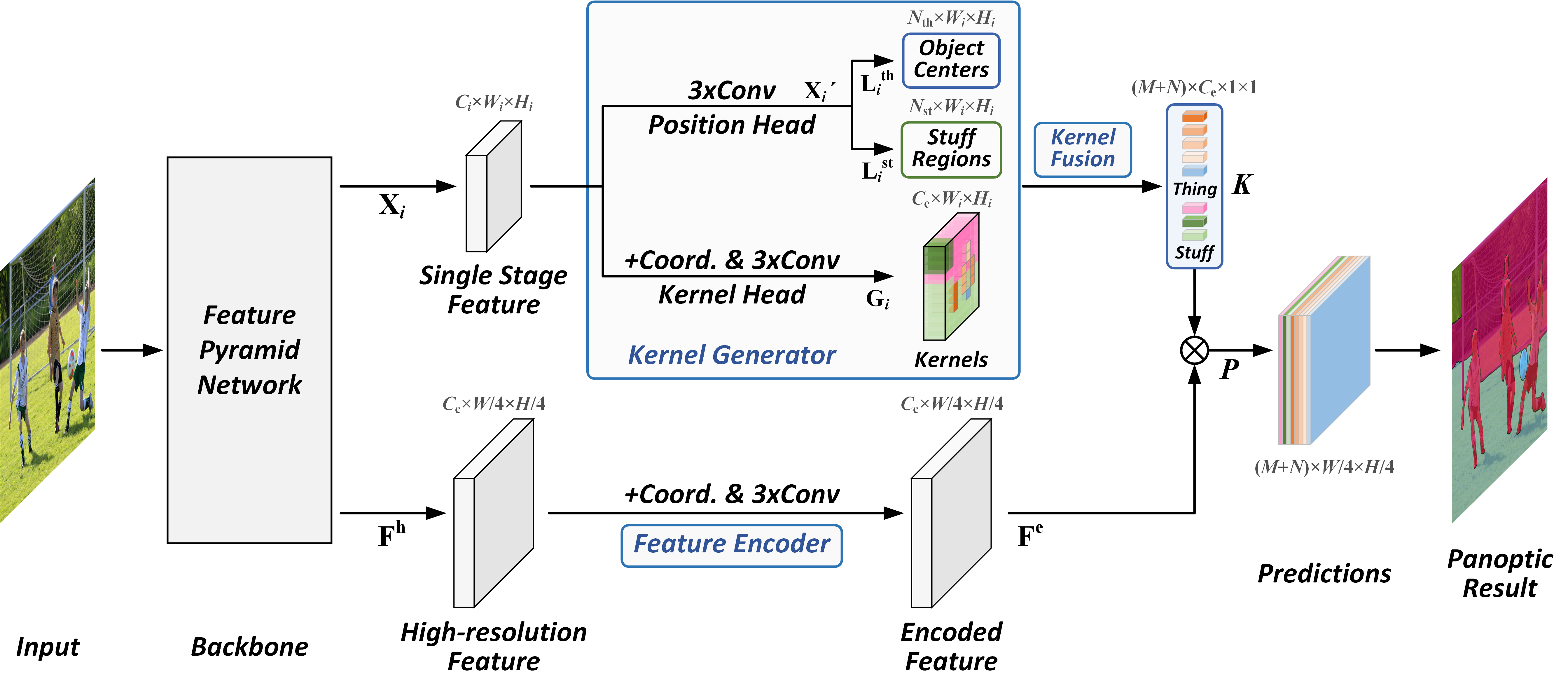
Figure 2: The framework of Panoptic FCN. The proposed framework mainly contains three components, namely kernel generator, kernel fusion, and feature encoder. In kernel generator, position head is designed to locate and classify object centers along with stuff regions; kernel head in each stage is used to generate kernel weights for both things and stuff. Then, kernel fusion is utilized to merge kernel weights with the same identity from different stages. And feature encoder is adopted to encode the high-resolution feature with details. With the generated kernel weight for each instance, both things and stuff can be predicted with a simple convolution directly. Best viewed in color.

3 Panoptic FCN

Panoptic FCN is conceptually simple: kernel generator is introduced to generate kernel weights for things and stuff with different categories; kernel fusion is designed to merge kernel weights with the same identity from multiple stages; and feature encoder is utilized to encode the high-resolution feature. In this section, we elaborate on the above components as well as the training and inference scheme.

3.1 Kernel Generator

Given a single stage feature $\mathbf{X}_{i}$ from the $i$-th stage in FPN [27], the proposed kernel generator aims at generating the kernel weight map $\mathbf{G}_{i}$ with positions for things $\mathbf{L}_{i}^{\mathrm{th}}$ and stuff $\mathbf{L}_{i}^{\mathrm{st}}$, as depicted in Fig. 2. To this end, position head is utilized for instance localization and classification, while kernel head is designed for kernel weight generation.

Position head.   With the input $\mathbf{X}_{i}\in\mathbb{R}^{C_{i}\times W_{i}\times H_{i}}$, we simply adopt stacks of convolutions to encode the feature map and generate $\mathbf{X}^{\prime}_{i}$, as presented in Fig. 2. Then we need to locate and classify each instance from the shared feature map $\mathbf{X}^{\prime}_{i}$. However, according to the definition [19], things can be distinguished by object centers, while stuff is uncountable. Thus, we adopt object centers and stuff regions to respectively represent position of each individual and stuff category. It means background regions with the same semantic meaning are viewed as one instance. In particular, object map $\mathbf{L}_{i}^{\mathrm{th}}\in\mathbb{R}^{N_{\mathrm{th}}\times W_{i}\times H_{i}}$ and stuff map $\mathbf{L}_{i}^{\mathrm{st}}\in\mathbb{R}^{N_{\mathrm{st}}\times W_{i}\times H_{i}}$ can be generated by convolutions directly with the shared feature map $\mathbf{X}^{\prime}_{i}$, where $N_{\mathrm{th}}$ and $N_{\mathrm{st}}$ denote the number of semantic category for things and stuff, respectively.

To better optimize $\mathbf{L}_{i}^{\mathrm{th}}$ and $\mathbf{L}_{i}^{\mathrm{st}}$, different strategies are adopted to generate the ground truth. For the $k$-th object in class $c$, we split positive key-points onto the $c$-th channel of the heatmap $\mathbf{Y}_{i}^{\mathrm{th}}\in\left[0,1\right]^{N_{\mathrm{th}}\times W_{i}\times H_{i}}$ with Gaussian kernel, similar to that in [20, 55]. With respect to stuff, we produce the ground truth $\mathbf{Y}_{i}^{\mathrm{st}}\in\left[0,1\right]^{N_{\mathrm{st}}\times W_{i}\times H_{i}}$ by bilinear interpolating the one-hot semantic label to corresponding sizes. Hence, the position head can be optimized with ${\mathcal{L}}_{\mathrm{pos}}^{\mathrm{th}}$ and ${\mathcal{L}}_{\mathrm{pos}}^{\mathrm{st}}$ for object centers and stuff regions, respectively.

$$~{}\begin{aligned} {\mathcal{L}}_{\mathrm{pos}}^{\mathrm{th}}=&\sum_{i}\mathrm{FL}(\mathbf{L}_{i}^{\mathrm{th}},\mathbf{Y}_{i}^{\mathrm{th}})/N_{\mathrm{th}},\\ {\mathcal{L}}_{\mathrm{pos}}^{\mathrm{st}}=&\sum_{i}\mathrm{FL}(\mathbf{L}_{i}^{\mathrm{st}},\mathbf{Y}_{i}^{\mathrm{st}})/{W_{i}H_{i}},\\ {\mathcal{L}}_{\mathrm{pos}}=&{\mathcal{L}}_{\mathrm{pos}}^{\mathrm{th}}+{\mathcal{L}}_{\mathrm{pos}}^{\mathrm{st}},\end{aligned}$$ (1)

where $\mathrm{FL}(\cdot,\cdot)$ represents the Focal Loss [28] for optimization. For inference, $D^{\mathrm{th}}_{i}=\left\{(x,y):\mathbbm{1}(\mathbf{L}^{\mathrm{th}}_{i,c,x,y})=1\right\}$ and $D^{\mathrm{st}}_{i}=\left\{(x,y):\mathbbm{1}(\mathbf{L}^{\mathrm{st}}_{i,c,x,y})=1\right\}$ are selected to respectively represent the existence of object centers and stuff regions in corresponding positions with predicted categories $O_{i}$. This process will be further explained in Sec. 3.4.

Kernel head. In kernel head, we first capture spatial cues by directly concatenating relative coordinates to the feature $\mathbf{X}_{i}$, which is similar with that in CoordConv [31]. With the concatenated feature map $\mathbf{X}^{\prime\prime}_{i}\in\mathbb{R}^{(C_{i}+2)\times W_{i}\times H_{i}}$, stacks of convolutions are adopted to generate the kernel weight map $\mathbf{G}_{i}\in\mathbb{R}^{C_{\mathrm{e}}\times W_{i}\times H_{i}}$, as presented in Fig. 2. Given predictions $D^{\mathrm{th}}_{i}$ and $D^{\mathrm{st}}_{i}$ from the position head, kernel weights with the same coordinates in $\mathbf{G}_{i}$ are chosen to represent corresponding instances. For example, assuming candidate $(x_{c},y_{c})\in D^{\mathrm{th}}_{i}$, kernel weight $\mathbf{G}_{i,:,x_{c},y_{c}}\in\mathbb{R}^{C_{\mathrm{e}}\times 1\times 1}$ is selected to generate the result with predicted category $c$. The same is true for $D^{\mathrm{st}}_{i}$. We represent the selected kernel weights in $i$-th stage for things and stuff as $G^{\mathrm{th}}_{i}$ and $G^{\mathrm{st}}_{i}$, respectively. Thus, the kernel weight $G^{\mathrm{th}}_{i}$ and $G^{\mathrm{st}}_{i}$ together with predicted categories $O_{i}$ in the $i$-th stage can be produced with the proposed kernel generator.

3.2 Kernel Fusion

Previous work [39, 12, 45] utilized NMS to remove duplicate boxes or instances in the post-processing stage. Different from them, the designed kernel fusion operation merges repetitive kernel weights from multiple FPN stages before final instance generation, which guarantees instance-awareness and semantic-consistency for things and stuff, respectively. In particular, given aggregated kernel weights $G^{\mathrm{th}}$ and $G^{\mathrm{st}}$ from all the stages, the $j$-th kernel weight $K_{j}\in\mathbb{R}^{C_{\mathrm{e}}\times 1\times 1}$ is achieved by

$$K_{j}=\mathrm{AvgCluster}(G_{j}^{\prime}),$$ (2)

where $\mathrm{AvgCluster}$ denotes average-clustering operation, and the candidate set $G_{j}^{\prime}=\{G_{m}:\mathrm{ID}(G_{m})=\mathrm{ID}(G_{j})\}$ includes all the kernel weights, which are predicted to have the same identity $\mathrm{ID}$ with $G_{j}$. For object centers, kernel weight $G^{\mathrm{th}}_{m}$ is viewed as identical with $G^{\mathrm{th}}_{j}$ if the cosine similarity between them surpasses a given threshold $thres$, which will be further investigated in Table 3. For stuff regions, all kernel weights in $G^{\mathrm{st}}$, which share a same category with $G^{\mathrm{st}}_{j}$, are marked as one identity $\mathrm{ID}$.

With the proposed approach, each kernel weight $K^{\mathrm{th}}_{j}$ in $K^{\mathrm{th}}=\{K^{\mathrm{th}}_{1},...,K^{\mathrm{th}}_{m}\}\in\mathbb{R}^{M\times C_{\mathrm{e}}\times 1\times 1}$ can be viewed as an embedding for single object, where the total number of objects is $M$. Therefore, kernels with the same identity are merged as a single embedding for things, and each kernel in $K^{\mathrm{th}}$ represents an individual object, which satisfies the instance-awareness for things. Meanwhile, kernel weight $K^{\mathrm{st}}_{j}$ in $K^{\mathrm{st}}=\{K^{\mathrm{st}}_{1},...,K^{\mathrm{st}}_{n}\}\in\mathbb{R}^{N\times C_{\mathrm{e}}\times 1\times 1}$ represents the embedding for all $j$-th class pixels, where the existing number of stuff is $N$. With this method, kernels with the same semantic category are fused into a single embedding, which guarantees the semantic-consistency for stuff. Thus, both properties requested by things and stuff can be fulfilled with the proposed kernel fusion operation.

3.3 Feature Encoder

To preserve details for instance representation, high-resolution feature $\mathbf{F}^{\mathrm{h}}\in\mathbb{R}^{C_{\mathrm{e}}\times W/4\times H/4}$ is utilized for feature encoding. Feature $\mathbf{F}^{\mathrm{h}}$ can be generated from FPN in several ways, e.g., P2 stage feature, summed features from all stages, and features from semantic FPN [18]. These methods are compared in Table 6. Given the feature $\mathbf{F}^{\mathrm{h}}$, a similar strategy with that in kernel head is applied to encode positional cues and generate the encoded feature $\mathbf{F}^{\mathrm{e}}\in\mathbb{R}^{C_{\mathrm{e}}\times W/4\times H/4}$, as depicted in Fig. 2. Thus, given $M$ and $N$ kernel weights for things $K^{\mathrm{th}}$ and stuff $K^{\mathrm{st}}$ from the kernel fusion, each instance is produced by $\mathbf{P}_{j}=K_{j}\otimes\mathbf{F}^{\mathrm{e}}$.

Here, $\mathbf{P}_{j}$ denotes the $j$-th prediction, and $\otimes$ indicates the convolutional operation. That means $M+N$ kernel weights generate $M+N$ instance predictions with resolution $W/4\times H/4$ for the whole image. Consequently, the panoptic result can be produced with a simple process [18].

3.4 Training and Inference

Training scheme. In the training stage, the central point in each object and all the points in stuff regions are utilized to generate kernel weights for things and stuff, respectively. Here, Dice Loss [34] is adopted to optimize the predicted segmentation, which is formulated as

$$~{}{\mathcal{L}}_{\mathrm{seg}}=\sum_{j}\mathrm{Dice}(\mathbf{P}_{j},\mathbf{Y}_{j}^{\mathrm{seg}})/(M+N),\\$$ (3)

where $\mathbf{Y}_{j}^{\mathrm{seg}}$ denotes ground truth for the $j$-th prediction $\mathbf{P}_{j}$. To further release the potential of kernel generator, multiple positives inside each object are sampled to represent the instance. In particular, we select $k$ positions with top predicted scores $s$ inside each object in $\mathbf{L}_{i}^{\mathrm{th}}$, resulting in $k\times M$ kernels as well as instances in total. This will be explored in Table 7. As for stuff regions, the factor $k$ is set to 1, which means all the points in same category are equally treated. Then, we replace the original loss with a weighted version

$$\mathrm{WDice}(\mathbf{P}_{j},\mathbf{Y}_{j}^{\mathrm{seg}})=\sum_{k}w_{k}\mathrm{Dice}(\mathbf{P}_{j,k},\mathbf{Y}_{j}^{\mathrm{seg}}),\\$$ (4)

where $w_{k}$ denotes the $k$-th weighted score with $w_{k}=s_{k}/\sum_{i}s_{i}$. According to Eqs. (1) and (3), optimized target ${\mathcal{L}}$ is defined with the weighted Dice Loss ${\mathcal{L}}_{\mathrm{seg}}$ as

$$~{}{\mathcal{L}}_{\mathrm{seg}}=\sum_{j}\mathrm{WDice}(\mathbf{P}_{j},\mathbf{Y}_{j}^{\mathrm{seg}})/(M+N),\\$$ (5)

$${\mathcal{L}}=\lambda_{\mathrm{pos}}{\mathcal{L}}_{\mathrm{pos}}+\lambda_{\mathrm{seg}}{\mathcal{L}}_{\mathrm{seg}}.$$ (6)

Inference scheme. In the inference stage, Panoptic FCN follows a simple generate-kernel-then-segment pipeline. Specifically, we first aggregate positions $D^{\mathrm{th}}_{i}$, $D^{\mathrm{st}}_{i}$ and corresponding categories $O_{i}$ from the $i$-th position head, as illustrated in the Sec. 3.1. For object centers, we preserve the peak points in $\mathrm{MaxPool}(\mathbf{L}^{\mathrm{th}}_{i})$ utilizing a similar method with that in [55]. Thus, the indicator for things $\mathbbm{1}(\mathbf{L}^{\mathrm{th}}_{i,c,x,y})$ is marked as positive if point $(x,y)$ in the $c$-th channel is preserved as the peak point. Similarly, the indicator for stuff regions $\mathbbm{1}(\mathbf{L}^{\mathrm{st}}_{i,c,x,y})$ is viewed as positive if point $(x,y)$ with category $c$ is kept. With the designed kernel fusion and the feature encoder, the prediction $\mathbf{P}$ can be easily produced. Specifically, we keep the top 100 scoring kernels of objects and all the kernels of stuff after kernel fusion for instance generation. The threshold 0.4 is utilized to convert predicted soft masks to binary results. It should be noted that both the heuristic process or direct $argmax$ could be used to generate non-overlap panoptic results. The $argmax$ could accelerate the inference but bring performance drop (1.4% PQ). For fair comparison both from speed and accuracy, the heuristic procedure [18] is adopted in experiments.

4 Experiments

In this section, we first introduce experimental settings for Panoptic FCN. Then we conduct abundant studies on the COCO [29] val set to reveal the effect of each component. Finally, comparison with previous methods on COCO [29], Cityscapes [8], and Mapillary Vistas [8] dataset is reported.

4.1 Experimental Setting

Architecture. From the perspective of network architecture, ResNet [13] with FPN [27] are utilized for backbone instantiation. P3 to P7 stages in FPN are used to provide single stage feature $\mathbf{X}_{i}$ for the kernel generator that is shared across all stages. Meanwhile, P2 to P5 stages are adopted to generate the high-resolution feature $\mathbf{F}^{\mathrm{h}}$, which will be further investigated in Table 6. All convolutions in kernel generator are equipped with $\mathrm{GroupNorm}$ [47] and $\mathrm{ReLU}$ activation. Moreover, a naive convolution is adopted at the end of each head in kernel generator for feature projection.

Datasets. COCO dataset [29] is a widely used benchmark, which contains 80 thing classes and 53 stuff classes. It involves 118K, 5K, and 20K images for training, validation, and testing, respectively. Cityscapes dataset [8] consists of 5,000 street-view fine annotations with size $1024\times 2048$, which are divided into 2,975, 500, and 1,525 images for training, validation, and testing, respectively. Mapillary Vistas [8] is a traffic-related dataset with resolutions ranging from $1024\times 768$ to more than $4000\times 6000$. It includes 37 thing classes and 28 stuff classes with 18K, 2K, and 5K images for training, validation, and testing, respectively.

Optimization. Network optimization is conducted using SGD with weight decay $1e^{-4}$ and momentum 0.9. And poly schedule with power 0.9 is adopted. Experimentally, $\lambda_{\mathrm{pos}}$ is set to a constant 1, and $\lambda_{\mathrm{seg}}$ are respectively set to 3, 4, and 3 for COCO, Cityscapes, and Mapillary Vistas datasets. For COCO, we set initial rate to 0.01 and follow the $1\times$ strategy in $\mathrm{Detectron2}$ [48] by default. We randomly flip and rescale the shorter edge from 640 to 800 pixels with 90K iterations. Herein, annotated object centers with instance scale range {(1,64), (32,128), (64,256), (128,512), (256,2048)} are assigned to P3-P7 stages, respectively. For Cityscapes, we optimize the network for 65K iterations with an initial rate 0.02 and construct each mini-batch with 32 random $512\times 1024$ crops from images that are randomly rescaled from 0.5 to 2.0$\times$. For Mapillary Vistas, the network is optimized for 150K iterations with an initial rate 0.02. In each iteration, we randomly resize images from 1024 to 2048 pixels at the shorted side and build 32 crops with the size $1024\times 1024$. Due to the variation in scale distribution, we modify the assigning strategy to {(1,128), (64,256), (128,512), (256,1024), (512,2048)} for Cityscapes and Mapillary Vistas datasets.

Table 1: Comparison with different settings of the kernel generator on the COCO val set. deform and conv num respectively denote deformable convolutions for position head and number of convolutions in both heads of the kernel generator.

deform	conv num	PQ	PQth	PQst	AP	mIoU
✗	1	38.4	43.4	31.0	28.3	39.9
✗	2	38.9	44.1	31.1	28.9	40.1
✗	3	39.2	44.7	31.0	29.6	40.2
✗	4	39.2	44.9	30.8	29.4	39.9
✓	3	39.9	45.0	32.4	29.9	41.2

Table 2: Comparison with different positional settings on the COCO val set. coord_w and coord_f denote combining coordinates for the kernel head, and feature encoder, respectively.

coordw	coordf	PQ	PQth	PQst	AP	mIoU
✗	✗	39.9	45.0	32.4	29.9	41.2
✓	✗	39.9	45.0	32.2	30.0	41.1
✗	✓	40.2	45.3	32.5	30.4	41.6
✓	✓	41.3	46.9	32.9	32.1	41.7

Table 3: Comparison with different similarity thresholds of kernel fusion on the COCO val set. class-aware denotes only merging kernel weights with the same predicted class. And thres indicates the cosine similarity threshold thres for kernel fusion in Sec. 3.2.

class-aware	thres	PQ	PQth	PQst	AP	mIoU
✓	0.80	39.7	44.3	32.9	29.9	41.7
✓	0.85	40.8	46.1	32.9	31.5	41.7
✓	0.90	41.3	46.9	32.9	32.1	41.7
✓	0.95	41.3	47.0	32.9	31.1	41.7
✓	1.00	38.7	42.6	32.9	25.4	41.7
✗	0.90	41.2	46.7	32.9	30.9	41.7

Table 4: Comparison with different methods of removing repetitive predictions. kernel-fusion and nms indicates the proposed kernel-level fusion method and Matrix NMS [46], respectively.

kernel-fusion	nms	PQ	PQth	PQst	AP	mIoU
✗	✗	38.7	42.6	32.9	25.4	41.7
✗	✓	38.7	42.6	32.9	27.8	41.7
✓	✗	41.3	46.9	32.9	32.1	41.7
✓	✓	41.3	46.9	32.8	32.3	41.7

4.2 Component-wise Analysis

Kernel generator. Kernel generator plays a vital role in Panoptic FCN. Here, we compare several settings inside kernel generator to improve the kernel expressiveness in each stage. As presented in Table 1, with the number of convolutions in each head increasing, the network performance improves steadily and achieves the peak PQ with 3 stacked $\mathrm{Conv3\times 3}$ whose channel number is 256. Similar with [55], deformable convolutions [56] are adopted in position head to extend the receptive field, which brings further improvement, especially in stuff regions (1.4% PQ).

Position embedding. Due to the instance-aware property of objects, position embedding is introduced to provide essential cues. In Table 2, we compare among several positional settings by attaching relative coordinates [31] to different heads. An interesting finding is that the improvement is minor (up to 0.3% PQ) if coordinates are attached to the kernel head or feature encoder only, but it boosts to 1.4% PQ when given the positional cues to both heads. It can be attributed to the constructed correspondence in the position between kernel weights and the encoded feature.

Table 5: Comparison with different channel numbers of the feature encoder on the COCO val set. channel num represents the channel number $C_{\mathrm{e}}$ of the feature encoder.

channel num	PQ	PQth	PQst	AP	mIoU
16	39.9	45.0	32.1	30.8	41.3
32	40.8	46.3	32.5	31.7	41.6
64	41.3	46.9	32.9	32.1	41.7
128	41.3	47.0	32.6	32.6	41.7

Table 6: Comparison with different feature types for the feature encoder on the COCO val set. feature type denotes the method to generate high-resolution feature $\mathbf{F}^{\mathrm{h}}$ in Sec. 3.3.

feature type	PQ	PQth	PQst	AP	mIoU
FPN-P2	40.6	46.0	32.4	31.6	41.3
FPN-Summed	40.5	46.0	32.1	31.7	41.1
Semantic FPN [18]	41.3	46.9	32.9	32.1	41.7

Table 7: Comparison with different settings of weighted dice loss on the COCO val set. weighted and $k$ denote weighted dice loss and the number of sampled points in Sec. 3.4, respectively.

weighted	$k$	PQ	PQth	PQst	AP	mIoU
✗	-	40.2	45.5	32.4	31.0	41.3
✓	1	40.0	45.1	32.4	30.9	41.4
✓	3	41.0	46.4	32.7	31.6	41.4
✓	5	41.0	46.5	32.9	32.1	41.7
✓	7	41.3	46.9	32.9	32.1	41.7
✓	9	41.3	46.8	32.9	32.1	41.8

Table 8: Comparison with different training schedules on the COCO val set. $\mathrm{1\times}$, $\mathrm{2\times}$, and $\mathrm{3\times}$ schedule denote the $\mathrm{90K}$, $\mathrm{180K}$, and $\mathrm{270K}$ training iterations in $\mathrm{Detectron2}$ [48], respectively.

schedule	PQ	PQth	PQst	AP	mIoU
$\mathrm{1\times}$	41.3	46.9	32.9	32.1	41.7
$\mathrm{2\times}$	43.2	48.8	34.7	34.3	43.4
$\mathrm{3\times}$	43.6	49.3	35.0	34.5	43.8

Table 9: Comparison with different settings of the feature encoder on the COCO val set. deform and channel num represent deformable convolutions and the channel number $C_{\mathrm{e}}$, respectively.

deform	channel num	PQ	PQth	PQst	AP	mIoU
✗	64	43.6	49.3	35.0	34.5	43.8
✓	256	44.3	50.0	35.6	35.5	44.0

Table 10: Upper-bound analysis on the COCO val set. gt position and gt class denote utilizing the ground-truth position $G_{i}$ and class $O_{i}$ in each position head for kernel generation, respectively.

gt position	gt class	PQ	PQth	PQst	AP	mIoU
✗	✗	43.6	49.3	35.0	34.5	43.8
✓	✗	49.8	52.2	46.1	38.2	54.6
✓	✓	65.9	64.1	68.7	45.5	86.6
		+22.3	+14.8	+33.7	+11.0	+42.8

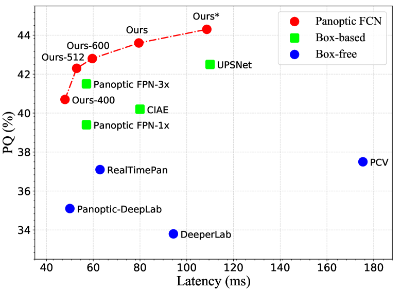
Figure 3: Speed-Accuracy trade-off curve on the COCO val set. All results are compared with Res50 except DeeperLab [51] based on Xception-71 [7]. The latency is measured end-to-end from single input to panoptic result. Details are given in Table 11.

Kernel fusion. Kernel fusion is a core operation in the proposed method, which guarantees the required properties for things and stuff, as elaborated in Sec. 3.2. We investigate the fusion type class-aware and similarity thresholds thres in Table 3. As shown in the table, the network attains the best performance with thres 0.90. And the class-agnostic manner could dismiss some similar instances with different categories, which yields drop in AP. Furthermore, we compare kernel fusion with Matrix NMS [46] which is utilized for pixel-level removal. As presented in Table 4, the performance saturates with the simple kernel-level fusion method, and extra NMS brings no more gain.

Table 11: Comparisons with previous methods on the COCO val set. Panoptic FCN-400, 512, and 600 denotes utilizing smaller input instead of the default setting. All our results are achieved on the same device with single input and no flipping. FPS is measured end-to-end from single input to panoptic result with an average speed over 1,000 images, which could be further improved with more optimizations. The simple enhanced version is marked with *. The model testing by ourselves according to released codes is denoted as †.

Method	Backbone	PQ	SQ	RQ	PQth	SQth	RQth	PQst	SQst	RQst	Device	FPS
box-based
Panoptic FPN [18]	Res50-FPN	39.0	-	-	45.9	-	-	28.7	-	-	-	-
Panoptic FPN†-$\mathrm{1\times}$	Res50-FPN	39.4	77.8	48.3	45.9	80.9	55.3	29.6	73.3	37.7	V100	17.5
Panoptic FPN†-$\mathrm{3\times}$	Res50-FPN	41.5	79.1	50.5	48.3	82.2	57.9	31.2	74.4	39.5	V100	17.5
AUNet [25]	Res50-FPN	39.6	-	-	49.1	-	-	25.2	-	-	-	-
CIAE [11]	Res50-FPN	40.2	-	-	45.3	-	-	32.3	-	-	2080Ti	12.5
UPSNet† [50]	Res50-FPN	42.5	78.0	52.5	48.6	79.4	59.6	33.4	75.9	41.7	V100	9.1
Unifying [24]	Res50-FPN	43.4	79.6	53.0	48.6	-	-	35.5	-	-	-	-
box-free
DeeperLab [51]	Xception-71	33.8	-	-	-	-	-	-	-	-	V100	10.6
Panoptic-DeepLab [6]	Res50	35.1	-	-	-	-	-	-	-	-	V100	20.0
AdaptIS [40]	Res50	35.9	-	-	40.3	-	-	29.3	-	-	-	-
RealTimePan [14]	Res50-FPN	37.1	-	-	41.0	-	-	31.3	-	-	V100	15.9
PCV [43]	Res50-FPN	37.5	77.7	47.2	40.0	78.4	50.0	33.7	76.5	42.9	1080Ti	5.7
SOLO V2 [46]	Res50-FPN	42.1	-	-	49.6	-	-	30.7	-	-	-	-
Panoptic FCN-400	Res50-FPN	40.7	80.5	49.3	44.9	82.0	54.0	34.3	78.1	42.1	V100	20.9
Panoptic FCN-512	Res50-FPN	42.3	80.9	51.2	47.4	82.1	56.9	34.7	79.1	42.7	V100	18.9
Panoptic FCN-600	Res50-FPN	42.8	80.6	51.6	47.9	82.6	57.2	35.1	77.4	43.1	V100	16.8
Panoptic FCN	Res50-FPN	43.6	80.6	52.6	49.3	82.6	58.9	35.0	77.6	42.9	V100	12.5
Panoptic FCN∗	Res50-FPN	44.3	80.7	53.0	50.0	83.4	59.3	35.6	76.7	43.5	V100	9.2

Feature encoder. To enhance expressiveness of the encoded feature $\mathbf{F}^{\mathrm{e}}$, we further explore the channel number and feature type used in feature encoder. As illustrated in Table 5, the network achieves 41.3% PQ with 64 channels, and extra channels contribute little improvement. For efficiency, we set the channel number of feature encoder to 64 by default. As for high-resolution feature generation, three types of methods are further discussed in Table 6. It is clear that Semantic FPN [18], which combines features from four stages in FPN, achieves the top performance 41.3% PQ.

Weighted dice loss. The designed weighted dice loss aims to release the potential of kernel generator by sampling $k$ positive kernels inside each object. Compared with the original dice loss, which selects a single central point in each object, improvement brought by the weighted dice loss reaches 1.1% PQ, as presented in Table 7. This is achieved by sampling 7 top-scoring kernels to generate results of each instance, which are optimized together in each step.

Training schedule. To fully optimize the network, we prolong the training iteration to the $3\times$ training schedule, which is widely adopted in recent one-stage instance-level approaches [4, 45, 46]. As shown in Table 8, $2\times$ training schedule brings 1.9% PQ improvements and increasing iterations to $3\times$ schedule contributes extra 0.4% PQ.

Enhanced version. We further explore model capacity by combining existing simple enhancements, e.g., deformable convolutions and extra channels. As illustrated in Table 9, the simple reinforcement contributes 0.7% improvement over the default setting, marked as Panoptic FCN*.

Upper-bound analysis. In Table 10, we give analysis to the upper-bound of generate-kernel-then-segment fashion with Res50-FPN backbone on the COCO val set. As illustrated in the table, given ground truth positions of object centers $\mathbf{L}_{i}^{\mathrm{th}}$ and stuff regions $\mathbf{L}_{i}^{\mathrm{st}}$, the network yields 6.2% PQ from more precise locations. And it will bring extra boost (16.1% PQ) to the network if we assign ground truth categories to the position head. Compared with the baseline method, there still remains huge potential to be explored (22.3% PQ in total), especially for stuff regions which could have even up to 33.7% PQ and 42.8% mIoU gains.

Speed-accuracy. To verify the network efficiency, we plot the end-to-end speed-accuracy trade-off curve on the COCO val set. As presented in Fig. 3, the proposed Panoptic FCN surpasses all previous box-free models by large margins on both performance and efficiency. Even compared with the well-optimized Panoptic FPN [18] from $\mathrm{Detectron2}$ [48], our approach still attains a better speed-accuracy balance with different image scales. Details about these data points are included in Table 11.

Table 12: Experiments on the COCO test-dev set. All our results are achieved with single scale input and no flipping. The simple enhanced version and val set for training are marked with * and ‡.

Method	Backbone	PQ	PQth	PQst
box-based
Panoptic FPN [18]	Res101-FPN	40.9	48.3	29.7
CIAE [11]	DCN101-FPN	44.5	49.7	36.8
AUNet [25]	ResNeXt152-FPN	46.5	55.8	32.5
UPSNet [50]	DCN101-FPN	46.6	53.2	36.7
Unifying‡ [24]	DCN101-FPN	47.2	53.5	37.7
BANet [5]	DCN101-FPN	47.3	54.9	35.9
box-free
DeeperLab [51]	Xception-71	34.3	37.5	29.6
SSAP [10]	Res101-FPN	36.9	40.1	32.0
PCV [43]	Res50-FPN	37.7	40.7	33.1
Panoptic-DeepLab [6]	Xception-71	39.7	43.9	33.2
AdaptIS [40]	ResNeXt-101	42.8	53.2	36.7
Axial-DeepLab [44]	Axial-ResNet-L	43.6	48.9	35.6
Panoptic FCN	Res101-FPN	45.5	51.4	36.4
Panoptic FCN	DCN101-FPN	47.0	53.0	37.8
Panoptic FCN∗	DCN101-FPN	47.1	53.2	37.8
Panoptic FCN∗‡	DCN101-FPN	47.5	53.7	38.2

Table 13: Experiments on the Cityscape val set. All our results are achieved with single scale input and no flipping. The simple enhanced version is marked with *.

Method	Backbone	PQ	PQth	PQst
box-based
Panoptic FPN [18]	Res101-FPN	58.1	52.0	62.5
AUNet [25]	Res101-FPN	59.0	54.8	62.1
UPSNet [50]	Res50-FPN	59.3	54.6	62.7
SOGNet [52]	Res50-FPN	60.0	56.7	62.5
Seamless [36]	Res50-FPN	60.2	55.6	63.6
Unifying [24]	Res50-FPN	61.4	54.7	66.3
box-free
PCV [43]	Res50-FPN	54.2	47.8	58.9
DeeperLab [51]	Xception-71	56.5	-	-
SSAP [10]	Res50-FPN	58.4	50.6	-
AdaptIS [40]	Res50	59.0	55.8	61.3
Panoptic-DeepLab [6]	Res50	59.7	-	-
Panoptic FCN	Res50-FPN	59.6	52.1	65.1
Panoptic FCN∗	Res50-FPN	61.4	54.8	66.6

Table 14: Experiments on the Mapillary Vistas val set. All our results are achieved with single scale input and no flipping. The simple enhanced version is marked with *.

Method	Backbone	PQ	PQth	PQst
box-based
BGRNet [49]	Res50-FPN	31.8	34.1	27.3
TASCNet [22]	Res50-FPN	32.6	31.1	34.4
Seamless [36]	Res50-FPN	36.2	33.6	40.0
box-free
DeeperLab [51]	Xception-71	32.0	-	-
AdaptIS [40]	Res50	32.0	26.6	39.1
Panoptic-DeepLab [6]	Res50	33.3	-	-
Panoptic FCN	Res50-FPN	34.8	30.6	40.5
Panoptic FCN∗	Res50-FPN	36.9	32.9	42.3

4.3 Main Results

We further conduct experiments on different scenarios, namely COCO dataset for common context, Cityscapes and Mapillary Vistas datasets for traffic-related environments.

COCO. In Table 11, we conduct experiments on COCO val set. Compared with recent approaches, Panoptic FCN achieves superior performance with efficiency, which surpasses leading box-based [24] and box-free [43] methods over 0.2% and 1.5% PQ, respectively. With simple enhancement, the gap enlarges to 0.9% and 2.2% PQ. Meanwhile, Panoptic FCN outperforms all top-ranking models on COCO test-dev set, as illustrated in Table 12. In particular, the proposed method surpasses the state-of-the-art approach in box-based stream with 0.2% PQ and attains 47.5% PQ with single scale inputs. Compared with the similar box-free fashion, our method improves 1.9% PQ over Axial-DeepLab [44] which adopts stronger backbone.

Cityscapes. Furthermore, we carry out experiments on Cityscapes val set in Table 13. Panoptic FCN exceeds the top box-free model [6] with 1.7% PQ and attains 61.4% PQ. Even compared with the leading box-based model [24], which utilizes Lovasz loss for further optimization, the proposed method still achieves comparable performance.

Mapillary Vistas. In Table 14, we compare with other state-of-the-art models on the large-scale Mapillary Vistas val set with Res50-FPN backbone. As presented in the table, the proposed Panoptic FCN exceeds previous box-free methods by a large margin in both things and stuff. Specifically, Panoptic FCN surpasses the leading box-based [36] and box-free [6] models with 0.7% and 3.6% PQ, and attains 36.9% PQ with simple enhancement in the feature encoder.

5 Conclusion

We have presented the Panoptic FCN, a conceptually simple yet effective framework for panoptic segmentation. The key difference from prior works lies on that we represent and predict things and stuff in a fully convolutional manner. To this end, kernel generator and kernel fusion are proposed to generate the unique kernel weight for each object instance or semantic category. With the high-resolution feature produced by feature encoder, prediction is achieved by convolutions directly. Meanwhile, instance-awareness and semantic-consistency for things and stuff are respectively satisfied with the designed workflow.

6 Acknowledgment

This research was partially supported by National Key R&D Program of China (No. 2017YFA0700800), and Beijing Academy of Artificial Intelligence (BAAI).

Appendix A Experimental Details

Herein, we provide more technical details of the training and inference process in the proposed Panoptic FCN.

A.1 Training Details

Position head. To better optimize the position head, we have explored different types of center assigning strategy. For object center generation, mass center is utilized to provide the $k$-th ground-truth coordinate $\widetilde{x}_{k}$ and $\widetilde{y}_{k}$ of the main paper. As presented in Table 15, compared with the box center for ground-truth generation, we find that mass center brings superior performance and higher robustness, especially in the designed weighted dice loss, which samples 7 top-scoring points inside each object. It could be attributed to that most of mass centers are located within the object area, while it is not the case for box centers. Moreover, the object size-adaptive deviation $\sigma_{k}$ of the main paper is set to $(2r+1)/3$, where $r$ denotes the gaussian radius of the $k$-th object similar to that in CornerNet [20].

Weighted dice loss. For objects, we select $k$ positions whose scores are predicted to be top-$k$ within the object region of $\mathbf{L}_{i,c}^{\mathrm{th}}$, where $c$ is the annotated class. This procedure utilizes $k$ top-scoring kernels to represent the same object and generates $k$ results of prediction $\mathbf{P}_{j}$. Thus, we generate the same ground-truth $\mathbf{Y}_{j}^{\mathrm{seg}}$ for $k$ results in $\mathbf{P}_{j}$, which can be optimized with Eq. (5). For stuff regions, we merge all positions with the same category in each stage using $\mathrm{AvgCluster}$, which brings a specific kernel. Hence, the factor $k$ can be viewed as 1 for each stuff region.

Table 15: Comparisons among different settings of center type on the COCO val set. weighted and center type denote weighted dice loss and center type for ground-truth generation, respectively.

weighted	center type	PQ	PQth	PQst	AP	mIoU
✗	box	39.7	44.7	32.3	30.3	41.2
✗	mass	40.2	45.5	32.4	31.0	41.3
✓	box	40.6	45.7	32.8	31.7	41.5
✓	mass	41.3	46.9	32.9	32.1	41.7

A.2 Inference Details.

Due to the variation of scale distribution among datasets, we simply modify some parameters in the inference stage. In particular, for COCO dataset, we preserve 100 top-scoring kernels for object prediction and utilize threshold 0.4 to convert soft masks to binary results, as illustrated in Sec. 3.4 of the main paper. For Cityscapes and Mapillary Vistas datasets, 200 kernels with top predicted scores are kept for object prediction, and cosine threshold 0.95 and mask threshold 0.5 are utilized to fuse repetitive kernels and convert binary masks, respectively. Meanwhile, a similar strategy with that in SOLO [45, 46] is adopted to adjust predicted object scores. Furthermore, our codes for training and inference will be released to provide more details.

Appendix B Qualitative Results

We further visualize qualitative results of Panoptic FCN on several datasets with common context and traffic-related scenarios, i.e., COCO, Cityscapes, and Mapillary Vistas.

COCO. As presented in Fig. 4, Panoptic FCN gives detailed characterization to the daily environment. Thanks to the pixel-by-pixel handling manner and unified representation, details in foreground things and background stuff can be preserved. Moreover, the proposed approach also validates its effectiveness on objects with various scales in Fig. 4.

Cityscapes. As for the street view, we visualize panoptic results on the Cityscapes val set, as illustrated in Fig. 5. In addition to the well-depicted cars and pedestrians, the proposed approach achieves satisfactory performance on slender objects, like street lamps and traffic lights.

Mapillary Vistas. In Fig. 6, we further present panoptic results on the Mapillary Vistas val set, which contains larger scales traffic-related scenes. It is clear in the figure that the proposed Panoptic FCN achieves surprising results, especially on vehicles and traffic signs. The coherence of qualitative results also reflects the fulfillment of instance-awareness and semantic-consistency in Panoptic FCN.

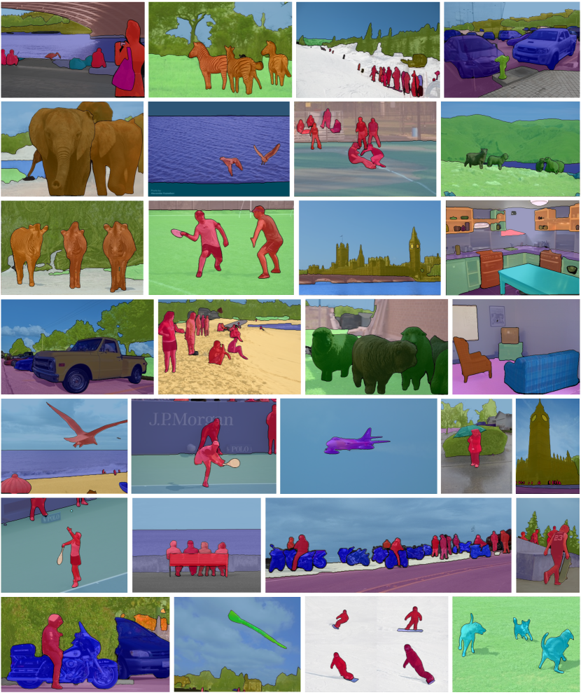
Figure 4: Visualization of panoptic results on the COCO val set.

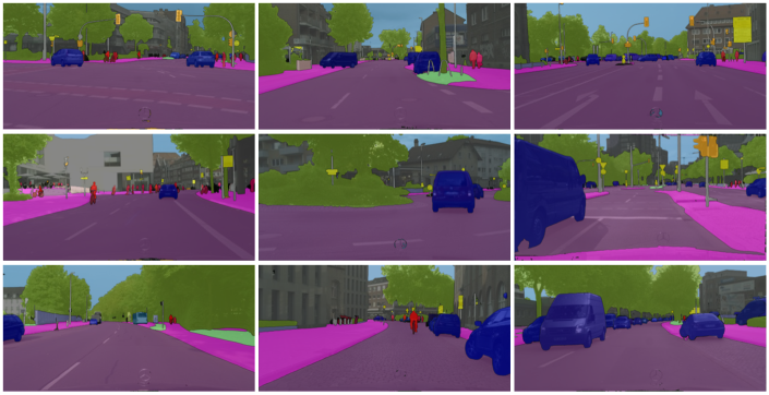
Figure 5: Visualization of panoptic results on the Cityscapes val set.

Figure 6: Visualization of panoptic results on the Mapillary Vistas val set.

References

- [1] Daniel Bolya, Chong Zhou, Fanyi Xiao, and Yong Jae Lee. Yolact: Real-time instance segmentation. In ICCV, 2019.
- [2] Liang-Chieh Chen, George Papandreou, Florian Schroff, and Hartwig Adam. Rethinking atrous convolution for semantic image segmentation. arXiv:1706.05587, 2017.
- [3] Liang-Chieh Chen, Yukun Zhu, George Papandreou, Florian Schroff, and Hartwig Adam. Encoder-decoder with atrous separable convolution for semantic image segmentation. In ECCV, 2018.
- [4] Xinlei Chen, Ross Girshick, Kaiming He, and Piotr Dollár. Tensormask: A foundation for dense object segmentation. In ICCV, 2019.
- [5] Yifeng Chen, Guangchen Lin, Songyuan Li, Omar Bourahla, Yiming Wu, Fangfang Wang, Junyi Feng, Mingliang Xu, and Xi Li. Banet: Bidirectional aggregation network with occlusion handling for panoptic segmentation. In CVPR, 2020.
- [6] Bowen Cheng, Maxwell D Collins, Yukun Zhu, Ting Liu, Thomas S Huang, Hartwig Adam, and Liang-Chieh Chen. Panoptic-deeplab: A simple, strong, and fast baseline for bottom-up panoptic segmentation. In CVPR, 2020.
- [7] François Chollet. Xception: Deep learning with depthwise separable convolutions. In CVPR, 2017.
- [8] Marius Cordts, Mohamed Omran, Sebastian Ramos, Timo Rehfeld, Markus Enzweiler, Rodrigo Benenson, Uwe Franke, Stefan Roth, and Bernt Schiele. The cityscapes dataset for semantic urban scene understanding. In CVPR, 2016.
- [9] Jun Fu, Jing Liu, Haijie Tian, Yong Li, Yongjun Bao, Zhiwei Fang, and Hanqing Lu. Dual attention network for scene segmentation. In CVPR, 2019.
- [10] Naiyu Gao, Yanhu Shan, Yupei Wang, Xin Zhao, Yinan Yu, Ming Yang, and Kaiqi Huang. Ssap: Single-shot instance segmentation with affinity pyramid. In ICCV, 2019.
- [11] Naiyu Gao, Yanhu Shan, Xin Zhao, and Kaiqi Huang. Learning category-and instance-aware pixel embedding for fast panoptic segmentation. arXiv:2009.13342, 2020.
- [12] Kaiming He, Georgia Gkioxari, Piotr Dollár, and Ross Girshick. Mask r-cnn. In ICCV, 2017.
- [13] Kaiming He, Xiangyu Zhang, Shaoqing Ren, and Jian Sun. Deep residual learning for image recognition. In CVPR, 2016.
- [14] Rui Hou, Jie Li, Arjun Bhargava, Allan Raventos, Vitor Guizilini, Chao Fang, Jerome Lynch, and Adrien Gaidon. Real-time panoptic segmentation from dense detections. In CVPR, 2020.
- [15] Han Hu, Jiayuan Gu, Zheng Zhang, Jifeng Dai, and Yichen Wei. Relation networks for object detection. In CVPR, 2018.
- [16] Zilong Huang, Xinggang Wang, Lichao Huang, Chang Huang, Yunchao Wei, and Wenyu Liu. Ccnet: Criss-cross attention for semantic segmentation. In ICCV, 2019.
- [17] Xu Jia, Bert De Brabandere, Tinne Tuytelaars, and Luc Van Gool. Dynamic filter networks. In NeurIPS, 2016.
- [18] Alexander Kirillov, Ross Girshick, Kaiming He, and Piotr Dollár. Panoptic feature pyramid networks. In CVPR, 2019.
- [19] Alexander Kirillov, Kaiming He, Ross Girshick, Carsten Rother, and Piotr Dollár. Panoptic segmentation. In CVPR, 2019.
- [20] Hei Law and Jia Deng. Cornernet: Detecting objects as paired keypoints. In ECCV, 2018.
- [21] Youngwan Lee and Jongyoul Park. Centermask: Real-time anchor-free instance segmentation. In CVPR, 2020.
- [22] Jie Li, Allan Raventos, Arjun Bhargava, Takaaki Tagawa, and Adrien Gaidon. Learning to fuse things and stuff. arXiv:1812.01192, 2018.
- [23] Qizhu Li, Anurag Arnab, and Philip HS Torr. Weakly-and semi-supervised panoptic segmentation. In ECCV, 2018.
- [24] Qizhu Li, Xiaojuan Qi, and Philip HS Torr. Unifying training and inference for panoptic segmentation. In CVPR, 2020.
- [25] Yanwei Li, Xinze Chen, Zheng Zhu, Lingxi Xie, Guan Huang, Dalong Du, and Xingang Wang. Attention-guided unified network for panoptic segmentation. In CVPR, 2019.
- [26] Yanwei Li, Lin Song, Yukang Chen, Zeming Li, Xiangyu Zhang, Xingang Wang, and Jian Sun. Learning dynamic routing for semantic segmentation. In CVPR, 2020.
- [27] Tsung-Yi Lin, Piotr Dollár, Ross Girshick, Kaiming He, Bharath Hariharan, and Serge Belongie. Feature pyramid networks for object detection. In CVPR, 2017.
- [28] Tsung-Yi Lin, Priya Goyal, Ross Girshick, Kaiming He, and Piotr Dollár. Focal loss for dense object detection. In ICCV, 2017.
- [29] Tsung-Yi Lin, Michael Maire, Serge Belongie, James Hays, Pietro Perona, Deva Ramanan, Piotr Dollár, and C Lawrence Zitnick. Microsoft coco: Common objects in context. In ECCV, 2014.
- [30] Chenxi Liu, Liang-Chieh Chen, Florian Schroff, Hartwig Adam, Wei Hua, Alan L Yuille, and Li Fei-Fei. Auto-deeplab: Hierarchical neural architecture search for semantic image segmentation. In CVPR, 2019.
- [31] Rosanne Liu, Joel Lehman, Piero Molino, Felipe Petroski Such, Eric Frank, Alex Sergeev, and Jason Yosinski. An intriguing failing of convolutional neural networks and the coordconv solution. In NeurIPS, 2018.
- [32] Shu Liu, Lu Qi, Haifang Qin, Jianping Shi, and Jiaya Jia. Path aggregation network for instance segmentation. In CVPR, 2018.
- [33] Jonathan Long, Evan Shelhamer, and Trevor Darrell. Fully convolutional networks for semantic segmentation. In CVPR, 2015.
- [34] Fausto Milletari, Nassir Navab, and Seyed-Ahmad Ahmadi. V-net: Fully convolutional neural networks for volumetric medical image segmentation. In 3DV, 2016.
- [35] Gerhard Neuhold, Tobias Ollmann, Samuel Rota Bulo, and Peter Kontschieder. The mapillary vistas dataset for semantic understanding of street scenes. In ICCV, 2017.
- [36] Lorenzo Porzi, Samuel Rota Bulo, Aleksander Colovic, and Peter Kontschieder. Seamless scene segmentation. In CVPR, 2019.
- [37] Lu Qi, Shu Liu, Jianping Shi, and Jiaya Jia. Sequential context encoding for duplicate removal. In NeurIPS, 2018.
- [38] Lu Qi, Xiangyu Zhang, Yingcong Chen, Yukang Chen, Jian Sun, and Jiaya Jia. Pointins: Point-based instance segmentation. arXiv:2003.06148, 2020.
- [39] Shaoqing Ren, Kaiming He, Ross Girshick, and Jian Sun. Faster r-cnn: Towards real-time object detection with region proposal networks. In NeurIPS, 2015.
- [40] Konstantin Sofiiuk, Olga Barinova, and Anton Konushin. Adaptis: Adaptive instance selection network. In ICCV, 2019.
- [41] Lin Song, Yanwei Li, Zeming Li, Gang Yu, Hongbin Sun, Jian Sun, and Nanning Zheng. Learnable tree filter for structure-preserving feature transform. In NeurIPS, 2019.
- [42] Zhi Tian, Chunhua Shen, and Hao Chen. Conditional convolutions for instance segmentation. arXiv preprint arXiv:2003.05664, 2020.
- [43] Haochen Wang, Ruotian Luo, Michael Maire, and Greg Shakhnarovich. Pixel consensus voting for panoptic segmentation. In CVPR, 2020.
- [44] Huiyu Wang, Yukun Zhu, Bradley Green, Hartwig Adam, Alan Yuille, and Liang-Chieh Chen. Axial-deeplab: Stand-alone axial-attention for panoptic segmentation. In ECCV, 2020.
- [45] Xinlong Wang, Tao Kong, Chunhua Shen, Yuning Jiang, and Lei Li. Solo: Segmenting objects by locations. In ECCV, 2020.
- [46] Xinlong Wang, Rufeng Zhang, Tao Kong, Lei Li, and Chunhua Shen. Solov2: Dynamic, faster and stronger. In NeurIPS, 2020.
- [47] Yuxin Wu and Kaiming He. Group normalization. In ECCV, 2018.
- [48] Yuxin Wu, Alexander Kirillov, Francisco Massa, Wan-Yen Lo, and Ross Girshick. Detectron2. https://github.com/facebookresearch/detectron2, 2019.
- [49] Yangxin Wu, Gengwei Zhang, Yiming Gao, Xiajun Deng, Ke Gong, Xiaodan Liang, and Liang Lin. Bidirectional graph reasoning network for panoptic segmentation. In CVPR, 2020.
- [50] Yuwen Xiong, Renjie Liao, Hengshuang Zhao, Rui Hu, Min Bai, Ersin Yumer, and Raquel Urtasun. Upsnet: A unified panoptic segmentation network. In CVPR, 2019.
- [51] Tien-Ju Yang, Maxwell D Collins, Yukun Zhu, Jyh-Jing Hwang, Ting Liu, Xiao Zhang, Vivienne Sze, George Papandreou, and Liang-Chieh Chen. Deeperlab: Single-shot image parser. arXiv:1902.05093, 2019.
- [52] Yibo Yang, Hongyang Li, Xia Li, Qijie Zhao, Jianlong Wu, and Zhouchen Lin. Sognet: Scene overlap graph network for panoptic segmentation. In AAAI, 2020.
- [53] Hengshuang Zhao, Jianping Shi, Xiaojuan Qi, Xiaogang Wang, and Jiaya Jia. Pyramid scene parsing network. In CVPR, 2017.
- [54] Hengshuang Zhao, Yi Zhang, Shu Liu, Jianping Shi, Chen Change Loy, Dahua Lin, and Jiaya Jia. Psanet: Point-wise spatial attention network for scene parsing. In ECCV, 2018.
- [55] Xingyi Zhou, Dequan Wang, and Philipp Krähenbühl. Objects as points. arXiv:1904.07850, 2019.
- [56] Xizhou Zhu, Han Hu, Stephen Lin, and Jifeng Dai. Deformable convnets v2: More deformable, better results. In CVPR, 2019.