Synchronizing subgrid scale models of turbulence to data

Abstract

Large Eddy Simulations of turbulent flows are powerful tools used in many engineering and geophysical settings. Choosing the right value of the free parameters for their subgrid scale models is a crucial task for which the current methods present several shortcomings. Using a technique called nudging we show that Large Eddy Simulations can synchronize to data coming from a high-resolution direct numerical simulation of homogeneous and isotropic turbulence. Furthermore, we found that the degree of synchronization is dependent on the value of the parameters of the subgrid scale models utilized, suggesting that nudging can be used as a way to select the best parameters for a model. For example, we show that for the Smagorinsky model synchronization is optimal when its constant takes the usual value of $0.16$. Analyzing synchronization dynamics puts the focus on reconstructing trajectories in phase space, contrary to traditional a posteriori tests of Large Eddy Simulations where the statistics of the flows are compared. These results open up the possibility of utilizing non-statistical analysis in a posteriori tests of Large Eddy Simulations.

I Introduction

Fluid turbulence, with its nonlinear and multiscale nature Davidson (2013); Frisch (1995), is a notoriously complicated and costly problem to solve numerically in a direct way. For these reasons, a whole array of turbulence models are regularly employed for both scientific research and industrial day-to-day tasks. Large Eddy Simulations (LES) are one particular family of models that achieve a good compromise between cost and accuracy and are widely used in engineering and geophysical applications. Their core approach consists of solving the larger scales of a fluid flow directly, while modeling the effects of the smaller eddies not resolved explicitly Meneveau and Katz (2000); Lesieur, Métais, and Comte (2005). The term modeled is the one associated with the stresses of the unresolved (or subgrid, as they are smaller than the computational grid) motions and the models, or closures, always introduce free parameters that must be set. In some cases, theoretical arguments can be used to determine the value of these parameters, as in the Lilly-Smagorinsky model for homogeneous and isotropic turbulence Smagorinsky (1963); Lilly (1967); Pope (2000). The usual approach though consists of comparing the models with data coming form either experiments or Direct Numerical Simulations (DNS) where all scales are resolved.

Tests of LES can be classified into a priori Piomelli, Moin, and Ferziger (1988); Buzzicotti et al. (2018) and a posteriori Cerutti and Meneveau (1998); Linkmann, Buzzicotti, and Biferale (2018); Biferale et al. (2019). The former approach consists of applying the models to filtered data generated in DNS or experiments to obtain a representation of how the stresses would look like in an LES and then compare against the true subgrid stresses, either by calculating the correlations between the two fields or comparing their one- Meneveau (1994) or two-points statistics Di Leoni et al. (2020). In the latter approach, actual LES are run and the results are compared against those of DNS or experiments, but as turbulence is chaotic these comparisons are usually solely statistical, as the different phase space trajectories do not match. Several tools coming from the data assimilation and optimization worlds are employed to effectively perform these comparisons and pick the results, such as Bayesian inference Kennedy and O’Hagan (2001); Chertkov et al. (2010); Héas et al. (2012); Pang et al. (2017); Bocquet et al. (2020), variational methods Rawlins et al. (2007); Wang, Wang, and Zaki (2019) and ensemble methods Anderson (2001); Ruiz, Pulido, and Miyoshi (2013); Mons, Wang, and Zaki (2019). But given the limitations of the testing methods and the high-dimensional and chaotic nature of turbulence, the questions of what is the best choice of parameters that best models a flow and how to find that value is not always clearly answered.

We approach the issue from a synchronization perspective Carrassi et al. (2008); Lalescu, Meneveau, and Eyink (2013) by using nudging Hoke and Anthes (1976); Lakshmivarahan and Lewis (2013); Di Leoni, Mazzino, and Biferale (2020). Nudging is a data assimilation method Kalnay (2003); Bauer, Thorpe, and Brunet (2015) that consists of adding a Newton relaxation term to the equations of motion with the purpose of nudging the flow to a prescribed field. The prescribed field is usually generated from data, either computational, experimental, or observational and the nudging term only acts where the data is available, i.e., the probe locations from where the data was extracted or the Fourier scales at which it was obtained. Nudging has been used to match boundary conditions in Numerical Weather Prediction von Storch, Langenberg, and Feser (2000); Waldron, Paegle, and Horel (1996); Miguez-Macho, Stenchikov, and Robock (2004) and has been shown to be capable of synchronizing a wide variety of flows to data Biswas et al. (2017); Foias, Mondaini, and Titi (2016); Albanez et al. (2016); Pazó, Carrassi, and López (2016); Farhat et al. (2019). Most importantly, nudging has proven to be effective at synchronizing three dimensional and fully developed turbulence Di Leoni, Mazzino, and Biferale (2020) and shows sensitivity to the value of the physical parameters of the flow Di Leoni, Mazzino, and Biferale (2018), meaning it can detect discrepancies between the data and the nudged flow.

In this work we harness the power of nudging to show that a LES can synchronize to DNS data and that the level of synchronization is dependant on the choice of parameters of the models. The flow of choice is homogeneous and isotropic turbulence and we test three different models: the classical Smagorinsky model, an Entropic Lattice Boltzmann inspired model and a Smagorinsky plus non-linear gradients model. In all three cases there exists an optimal choice of parameters that maximizes the degree of synchronization. The paper is structured as follow, in section II we introduce the three subgrid scales models considered in the work, how the nudging term can be added to the LES equations and the numerical set-up used in our simulations. In section III we present numerical results and in section IV we discuss our main conclusions.

II Equations and methods

II.1 Large Eddy Simulations

Incompressible fluid flow motion is described by the Navier-Stokes equations (NSE),

$$\frac{\partial u_{i}}{\partial t}+u_{k}\frac{\partial u_{i}}{\partial x_{k}}=-\frac{\partial p}{\partial x_{i}}+\nu\frac{\partial^{2}u_{i}}{\partial x^{2}_{k}},$$ (1)

where $\bm{u}$ is the three dimensional velocity field, $p$ is the pressure (divided by the density) and $\nu$ is the kinematic viscosity, plus the incompressibility condition

$$\frac{\partial u_{i}}{\partial x_{i}}=0,$$ (2)

and corresponding initial and boundary conditions.

Given a filtering operator $\mathcal{F}$ which filters out motions smaller than a prescribed length $\Delta$, the LES equations are obtained by applying $\mathcal{F}$ to the NSE, resulting in

$$\frac{\partial\tilde{u}_{i}}{\partial t}+\tilde{u}_{k}\frac{\partial\tilde{u}_{i}}{\partial x_{k}}=-\frac{\partial\tilde{p}}{\partial x_{i}}+\nu\frac{\partial^{2}\tilde{u}_{i}}{\partial x^{2}_{k}}-\frac{\partial\tau_{ik}}{\partial x_{k}},$$ (3)

where $\tilde{u}_{i}=\mathcal{F}(u_{i})$, $\tilde{p}=\mathcal{F}(p)$ and

$$\tau_{ij}= \mathcal{F}(u_{i}u_{j})-\mathcal{F}(u_{i})\mathcal{F}(u_{j})$$ (4)

$$-\frac{1}{3}\left(\mathcal{F}(u_{i}u_{i})-\mathcal{F}(u_{i})^{2}\right)\delta_{ij},$$

$$\tilde{p}=\mathcal{F}(p)+\frac{1}{3}\left(\mathcal{F}(u_{i}u_{i})-\mathcal{F}(u_{i})^{2}\right),$$ (5)

are the deviatoric part of the subgrid-scale stresses and the modified pressure, respectively. The incompressibility condition simply becomes the divergence free condition but for the filtered velocity fields.

As the subgrid-scale stresses depend on the product of unfiltered fields, the equations are closed by modeling $\tau_{ij}$ in terms of the filtered variables. In this work we analyze three different models. The first one is the classic Smagorinsky model

$$\tau^{S}_{ij}=-2\nu_{S}\tilde{S}_{ij},$$ (6)

where

$$\tilde{S}_{ij}=\frac{1}{2}\left(\frac{\partial\tilde{u}_{i}}{\partial x_{j}}+\frac{\partial\tilde{u}_{j}}{\partial x_{i}}\right),$$ (7)

are the filtered strain rates and

$$\nu_{S}=(c_{S}\Delta)^{2}\sqrt{2\tilde{S}_{kl}\tilde{S}_{kl}}$$ (8)

is the eddy viscosity Lilly (1967). The model has only one free parameter, the Smagorinsky constant $c_{S}$. In homogeneous and isotropic turbulence this constant usually takes values around $0.16$ Meneveau and Katz (2000).

The second model that we consider comes from the macroscopic formulation of the Entropic Lattice Boltzmann Model (ELBM) Karlin, Ferrante, and Öttinger (1999); Ansumali and Karlin (2002). In particular, we define the modeled subgrid stress tensor as,

$$\tau^{E}_{ij}=-2\nu_{E}\tilde{S}_{ij},$$ (9)

where the eddy viscosity now takes the interesting formulation derived in Malaspinas, Deville, and Chopard (2008),

$$\nu^{E}_{e}=(c_{E}\Delta)^{2}\frac{S_{\lambda\mu}S_{\mu\gamma}S_{\gamma\lambda}}{S_{\gamma\delta}S_{\gamma\delta}},$$ (10)

we will refer to this model as the ‘Entropic’ model hereafter. What makes $\nu^{E}_{e}$ particularly attractive is that it is not only proportional to the stress tensor as the Smagorinsky eddy viscosity but it results also in a non-positive definite subgrid scales closure. This means that the modeled subgrid tensor $\tau^{E}_{ij}$ as the exact one $\tau_{ij}$ can produce backscatter events of energy going to the resolved scales and not only from the resolved to the subgrid scales with a dissipative effect Waleffe (1992); Fang et al. (2012); Biferale, Musacchio, and Toschi (2012); Chen, Chen, and Eyink (2003). This model too only has one free parameter, $c_{E}$.

The third and last model that we considered consists in a combination between the Smagorinsky closure and the non-linear gradient or tensor eddy viscosity model, as discussed in Meneveau and Katz (2000),

$$(c_{nl}\Delta)^{2}\frac{\partial\tilde{u}_{i}}{\partial x_{k}}\frac{\partial\tilde{u}_{j}}{\partial x_{k}}.$$ (11)

As in the Entropic case, the gradient term is able to produce backscattering of energy. If this term is implemented just by itself simulations do not dissipate enough energy and typically produce inaccurate results. Therefore, the purely dissipative Smagorinsky terms is added to ensure stability. Following this idea, the mixed model can be written as

$$\tau^{nl}_{ij}=(c_{nl}\Delta)^{2}\frac{\partial\tilde{u}_{i}}{\partial x_{k}}\frac{\partial\tilde{u}_{j}}{\partial x_{k}}-(c_{S}\Delta)^{2}\sqrt{2\tilde{S}_{kl}\tilde{S}_{kl}}\,\,\tilde{S}_{ij}.$$ (12)

Contraty to other two cases, this model has two free parameters, $c_{nl}$ and $c_{S}$.

Traditionally, methods to estimate the values of the free parameters of every model can be classified into a priori and a posteriori approaches. In a priori methods data coming from either a DNS or experiments is first used to calculate the exact subgrid-scale stresses $\tau_{ij}$ as defined in (4), and then used to calculate the stresses according to the model being studied, finally the two fields are compared. While point-wise comparisons such as correlation coefficients and mean errors are commonly performed, these do not carry much prognosis power when it comes to predicting the statistic of a LES. Statistical comparisons, like comparing mean energy dissipation Meneveau (1994) or two-point correlations Di Leoni et al. (2020), have firmer foundations but still deal with filtered exact fields and not actual LES solutions. On the other hand, a posteriori approaches work by comparing the resulting flow statistics obtained by both DNS (and/or experiments) and LES. As turbulence is chaotic, the phase space trajectories coming from the different simulations can only be compared in a statistical sense. Methods such as ensemble Kalman filters Evensen (2006); Houtekamer and Zhang (2016) and variational optimization Talagrand and Courtier (1987); Rawlins et al. (2007) are then used to analyze the a posteriori simulations and find the optimal parameters.

II.2 Nudging the LES equations

Nudging is a data assimilation method based on adding a penalization term to the equations of motion with the purpose of keeping the evolution close to some data provided. In the context of LES, the nudging protocol takes the form:

$$\frac{\partial\tilde{u}_{i}}{\partial t}+\tilde{u}_{k}\frac{\partial\tilde{u}_{i}}{\partial x_{k}}=-\frac{\partial\tilde{p}}{\partial x_{i}}+\nu\frac{\partial^{2}\tilde{u}_{i}}{\partial x^{2}_{k}}-\frac{\partial\tau_{ki}}{\partial x_{k}}-\alpha\mathcal{I}(\tilde{u}_{i}-\tilde{u}^{\rm ref}_{i}),$$ (13)

where $\tilde{\bm{u}}^{\rm ref}$ is the reference data provided, $\mathcal{I}$ is a filtering operator that acts only where data is provided, and $\alpha$ is the magnitude of the nudging term.

Nudging will make the flow try to follow the data along the specific dynamical trajectory of the reference simulation. Nudging has been shown to be able to synchronize turbulence, both partially and fully, and is sensitive to the choice of parameters Di Leoni, Mazzino, and Biferale (2018, 2020).

II.3 Numerical set-up

The reference data was generated by solving Eq. (1) on a periodic cubic box using a pseudospectral approach with an Adams-Bashfort two-step method for the time integration and the $2/3$ rule for dealising. The grid had $N_{data}^{3}=2048^{3}$ points, the time step was equal to $dt=5\cdot 10^{-5}$. The size of the computational box is $2\pi$ and the the integral length is $L=1.1$. An isotropic, constant in time forcing term, $F$, acting only on the large scales $k_{f}=[1,2]$, was added to the RHS of Eq. (1). The characteristic speed of the flow is $U=0.92$. The viscosity used was equal to $\nu=1.6\cdot 10^{-4}$. The resulting Reynolds number $Re=UL/\nu$ is of the order of $6300$ and eddy turnover time is $T=L/U=1.22$.

The data from the fully resolved simulation were then filtered and used as reference, $\tilde{u}^{\rm ref}_{i}$, to nudge the LES equations (13) with the different models. The filter operators $\mathcal{F}$ and $\mathcal{I}$ used were both identical sharp Fourier cut-off filters

$$\mathcal{F}(\bm{u}(\bm{x},t))=\mathcal{I}(\bm{u}(\bm{x},t))=\sum_{|\bm{k}|\leq k_{n}}\hat{\bm{u}}(\bm{k},t)e^{i\bm{k}\cdot\bm{x}}$$ (14)

with $k_{n}=85$. The LES are performed with the same pseudo-spectral fully dealiased approach on the same periodic domain of size $2\pi$ but with a spatial resolution of $N^{3}=256^{3}$ grid points, resulting in a maximum wavenumber equal to $k_{n}$. Nudging does not need to have reference information available at every scale in order to work in more general settings Di Leoni, Mazzino, and Biferale (2020), but as we are interested in analyzing how the different scales synchronize and as the subgrid models activity is concentrated in the smaller scales, we nudge over the whole range of resolved scales. All simulations are forced with the same isotropic constant forcing mechanisms acting only on the large system scales ($k_{f}=[1,2]$). The choice of using the same deterministic forcing mechanism in both LES and reference simulations allows us to highlight the effects produced by the modeling of the subgrid term on the dynamics of the LES resolved scales. The value of the nudging amplitude $\alpha$ was always set to $10$ except when noted. The first snapshot of the fully resolved simulation, filtered as described in Eq. 14, was used as an initial condition in all LES simulations.

III Results

III.1 Smagorinsky model

In Fig. 1 we show the evolution of the kinetic energy of the reference simulation and of three nudged Smagorinsky simulations with different values of $c_{S}$. The figure inset shows a close up to the very early stages of the simulations. As the nudging acts on every resolved scale, none of the three nudged simulations have any trouble synchronizing, i.e. following, the reference simulation, although they all have distinct and different evolutions. All nudged simulations have a total energy which is slightly lower than the reference case, as was already observed in Di Leoni, Mazzino, and Biferale (2020). Let us stress that the nudging term allows the LES simulation to follow the reference data also when there is no subgrid scales model, see the red curve in Fig. 1 for $c_{S}=0$, acting itself as closure for the subgrid dynamics. The question then is: for which value of the free parameter the LES model synchronizes better?

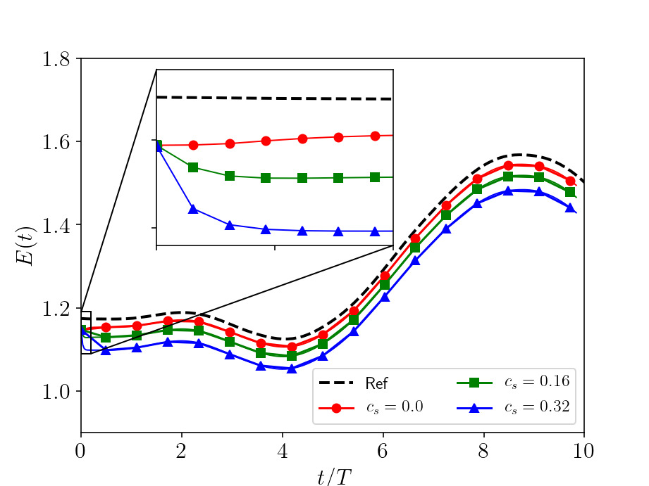
Figure 1: Energy evolution in time for the reference simulation at a resolution of $2048^{3}$ grid points (black dashed line) and for three different LES simulations equipped with the Smagorinsky closure at changing of the model free parameter, $c_{S}$.

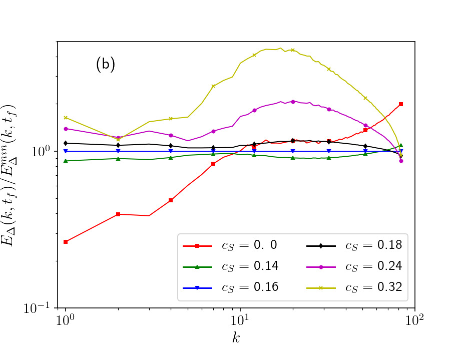
Figure 2: Panel (a): Energy spectra, $E(k,t_{f})$, of the reference simulation at a resolution of $2048^{3}$ grid points (black dashed line) and for the nudged LES simulations with a Smagorinsky closure at a resolution of $256^{3}$ grid points for different values of $c_{S}$. In the inset of the same figure we show the spectra of the difference, $E_{\Delta}(k,t_{f})$, measured for the same simulations of the main panel and compared with the energy spectra of the reference simulation. Panel (b): The spectra of the difference normalized by the $E_{\Delta}(k,t_{f})$ measured at $c_{S}=0.16$, the blue lines with downward triangles is equal to $1$ by definition.

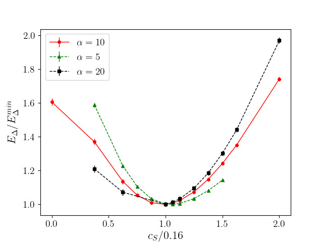
Figure 3: Time averaged relative errors, $E_{\Delta}$, for different amplitudes of the free parameter in the Smagorinsky model, $c_{S}$. The x- and y-axis are normalized respectively by $0.16$ and the relative error measured at $c_{S}=0.16$. The LES simulations where performed with different amplitudes of the nudging term, $\alpha=5$ (green line with triangles), $\alpha=10$ (red line with circles) and $\alpha=20$ (black line with squares).

In Fig. 2(a) we show the energy spectra,

$$E(k,t)=\frac{1}{2}\sum_{k\leq|\bm{k}|\leq k+1}|\hat{\bm{u}}(\bm{k},t)|^{2},$$ (15)

at the final time of the simulations, $t_{f}$ (see Fig. 1) for the reference flow and six nudged Smagorinsky simulations with different values of $c_{S}$. The spectra of the different nudged cases all coincide with the reference over almost the whole range of scales, differences between the different runs can be appreciated only at the highest wavenumbers. While the nudged simulation with $c_{S}=0$ is the one whose spectra is the closest to the reference one, it is important to remember that here we are only comparing the total amount of energy at each scale, not the actual configuration. To that end we calculate the spectra of the differences

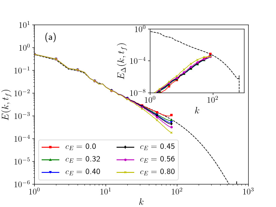
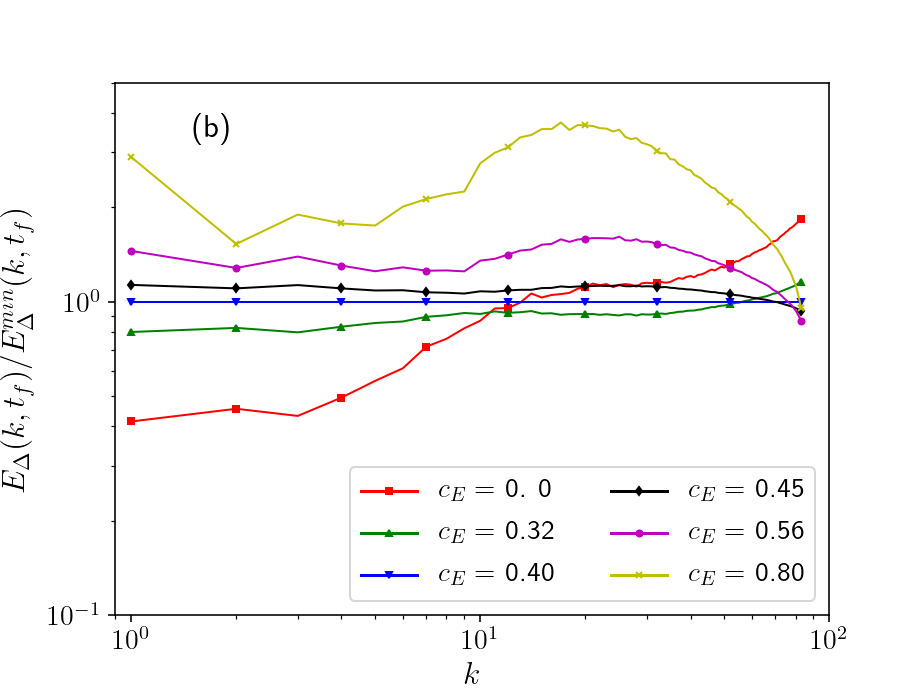
Figure 4: Panel (a): Energy spectra, $E(k,t_{f})$, of the reference simulation at a resolution of $2048^{3}$ grid points (black dashed line) and for the nudged LES simulations with the Entropic model closure at a resolution of $256^{3}$ grid points for different values of $c_{E}$. In the inset of the same figure we show the spectra of the difference, $E_{\Delta}(k,t_{f})$, measured for the same simulations of the main panel and compared with the energy spectra of the reference simulation. Panel (b): The spectra of the difference normalized by the $E_{\Delta}(k,t_{f})$ measured at $c_{E}=0.40$, the blue lines with downward triangles is equal to $1$ by definition.

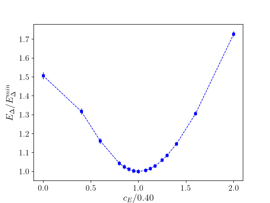
Figure 5: Time averaged relative errors, $E_{\Delta}$, for different amplitudes of the free parameter in the Entropic model, $c_{E}$. The x- and y-axis are normalized respectively by $0.40$ and the relative error measured at $c_{E}=0.40$. The LES simulations where performed with nudging amplitude $\alpha=10$.

$$E_{\Delta}(k,t)=\frac{1}{2}\sum_{k\leq|\bm{k}|\leq k+1}|\hat{\bm{u}}(\bm{k},t)-\hat{\bm{u}}^{\rm ref}(\bm{k},t)|^{2},$$ (16)

and show it in Fig. 2(a) alongside the spectra of the reference simulation (evaluted at final time $t_{f}$), while in Fig. 2(b) we show the same spectra (except for the reference one) but all normalized by the spectrum of the case with $c_{S}=0.16$, whose integral, i.e., total error, was found to be the smallest, as we discuss in detail below. Notice that the quantity $E_{\Delta}(k,t)$ tracks the kinetic energy of the difference of the two fields, not the difference of the energies of the two fields, and, as such, also takes into consideration any phase difference the Fourier coefficients of the two fields may have. These two figures show us how the models with lower values of $c_{S}$ do a slightly better job at synchronizing the largest scales of the flow but have problems at the smallest scales (compared to the case with $c_{S}=0.16$). On the other hand, simulations with a very high value of $c_{S}$ can have problems at all scales. This result suggests that the larger scales are less affected by the absence of the subgrid scales in the LES simulations, and their dynamics do not require any model. On the other hand, moving towards the filter cutoff, the missing degrees of freedom devolve on a larger deviation in the dynamics of such scales and the model becomes necessary. Let us stress once more that having found that the modelled LES can be synchronized to fully resolved simulations, now our aim to find the optimal parameters choice that maximizes the level of synchronization.

Finally, in Fig. 3 we make a global quantitative assessment of how well each simulation is synchronizing to the reference by showing the values of the time averaged relative errors $E_{\Delta}=\langle\sum_{1<k<k_{\eta}}E_{\Delta}(k,t)\rangle$ (where $\langle.\rangle$ denotes the time average) normalized by the value of $E_{\Delta}$ for the case with $c_{S}=0.16$ scanned over a range of $c_{S}$ and using different values of the nudging amplitude $\alpha$. Errorbars in the figure were obtained by calculating the standard deviation of $\sum_{1<k<k_{\eta}}E_{\Delta}(k,t)$. The dependence on $\alpha$ can be explained as follows. When $\alpha$ is too small the nudging term is less effective and the LES model is required to ensure stability at small scales, indeed, the error grows quickly when $c_{S}$ is too small (see green line with triangles). On the contrary, when $\alpha$ is large, the small scales stability is guaranteed by nudging also very small $c_{S}$, however in this case the simulations show larger deviations when increasing $c_{S}$, suggesting that synchronization becomes more sensitive to the error introduced at large scales by the model (see black line with squares). For all three scans, the lowest values are encountered when $c_{S}\approx 0.16$, in agreement with other statistical estimations based on a priori and a posteriori tests and on theoretical arguments Meneveau and Katz (2000). As expected too, the minimum around $0.16$ is not extremely sharp, as LES are known to produce accurate results with slightly different values of $c_{S}$.

III.2 Entropic model

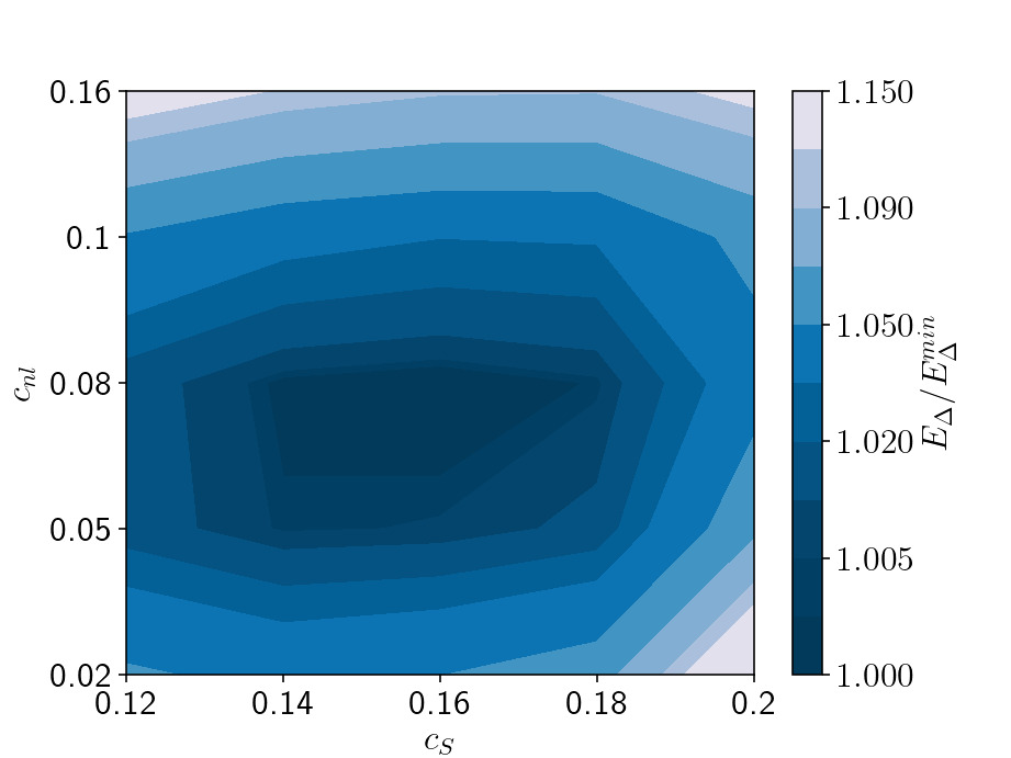
Figure 6: Time averaged relative error, normalized to its minimum, as a function of the non-linear model parameters, $(c_{S},c_{nl})$.

We now repeat the same analysis as above but for the Entropic model outlined in Eq. (10). In Fig. 4(a) we show the energy spectra at the final time of the simulations for the reference flow and six nudged Entropic simulations with different values of $c_{E}$. Again, the spectra of the different nudged cases all coincide with the reference over almost the whole range of scales, differences between the different runs can be appreciated only at the highest wavenumbers. In the inset of the same figure we show the spectra of the differences $E_{\Delta}(k,t_{f})$, alongside the spectra of the reference simulation, while in Fig. 4(b) we show the same spectra (except for the reference one) but normalized by the spectrum of the case with $c_{E}=0.40$. The results are very similar to what is observed for the Smagorinsky model, indicating that synchronization between LES and fully resolved data is possible not only for the specific case of the Smagorinsky model.

In Fig. 5 we show a scan of the time averaged total error $E_{\Delta}$ as a function of $c_{E}$. As with the previous case, the x- and y-axis are normalized respectively by the value of $c_{E}=0.40$ and its corresponding error, that is the value able to synchronize more closely to the reference data. Let us stress that while in the Smagorinsky case nudging provided us a result in agreement with the previous literature, this is the first time that the Entropic model has been used in a LES simulation, proving how nudging can be used to fit free parameters in new models.

III.3 Smagorinsky model with nonlinear gradients

Before concluding, we analyze the nudged LES simulations performed using the non-linear model, namely the Smagorinsky model plus the gradients term, outlined in Eq. (12). The reasons for choosing this third model are twofold. First, we wanted to investigate the possibility for nudged LES to synchronize with reference data also in the presence of more complex/non-linear models. Second, the non-linear model has two free parameters and it is interesting to understand if synchronization shows a minimum also in this 2-dimensional phase-space, $(c_{S},c_{nl})$. Results are summarized in Fig. 6, where we show the time averaged relative errors, $E_{\Delta}$, measured scanning the $(c_{S},c_{nl})$-space. We can conclude that also in this case the LES were able to synchronize with respect to the reference data, and that the relative averaged error presents a clear minimum around the point $(c_{S}=0.16,c_{nl}=0.07)$. This result further support the observation that LES can synchronize with reference data independently of the specific properties of model used.

IV Conclusions

We have shown that it is possible to synchronize a LES to data coming from a fully resolved simulation of homogeneous and isotropic turbulence, meaning that the LES can follow the particular trajectory of a fully resolved case. The analysis was repeated using three different models yielding successful results in all cases. Even more interestingly, we have shown that by varying the model parameters it is possible to change the level of synchronization between the LES and data, and that for each model there exists an optimal choice of parameters that minimizes the distance between the LES and the data. Therefore, nudging offers a way to get an estimate of the optimal model parameters that relies on reconstructing specific trajectories in phase space. We have also shown how nudging allows to have a scale-by-scale estimation of the errors introduced by the models considered. These results open up new ways in which to test LES models and choose their parameters. While in its current form the nudging algorithm presented lacks a proper optimization procedure to iterate over the parameters, the powers of synchronization could also be harnessed by different data assimilation and optimization methods.

Data Availability

The data that support the findings of this study are available from the corresponding author upon reasonable request.

References

- Davidson (2013) P. A. Davidson, Turbulence in Rotating, Stratified and Electrically Conducting Fluids (Cambridge University Press, 2013).
- Frisch (1995) U. Frisch, Turbulence : the legacy of A.N. Kolmogorov (Cambridge University Press, 1995) p. 296.
- Meneveau and Katz (2000) C. Meneveau and J. Katz, “Scale-Invariance and Turbulence Models for Large-Eddy Simulation,” Annual Review of Fluid Mechanics 32, 1–32 (2000).
- Lesieur, Métais, and Comte (2005) M. Lesieur, O. Métais, and P. Comte, Large-eddy simulations of turbulence (Cambridge University Press, 2005).
- Smagorinsky (1963) J. Smagorinsky, “General circulation experiments with the primitive equations: I. the basic experiment.” Monthly weather review 91, 99–164 (1963).
- Lilly (1967) D. K. Lilly, “The representation of small scale turbulence in numerical simulation experiments,” in Proc. IBM Scientific Computing Symposium on environmental sciences, edited by H. H. Goldstine (1967) pp. 195–210.
- Pope (2000) S. B. Pope, Turbulent Flows (Cambridge University Press, 2000).
- Piomelli, Moin, and Ferziger (1988) U. Piomelli, P. Moin, and J. H. Ferziger, “Model consistency in large eddy simulation of turbulent channel flows,” Phys. Fluids 31, 1884–1891 (1988).
- Buzzicotti et al. (2018) M. Buzzicotti, M. Linkmann, H. Aluie, L. Biferale, J. Brasseur, and C. Meneveau, “Effect of filter type on the statistics of energy transfer between resolved and subfilter scales from a-priori analysis of direct numerical simulations of isotropic turbulence,” Journal of Turbulence 19, 167–197 (2018).
- Cerutti and Meneveau (1998) S. Cerutti and C. Meneveau, “Intermittency and relative scaling of subgrid-scale energy dissipation in isotropic turbulence,” Phys. Fluids 10, 928 (1998).
- Linkmann, Buzzicotti, and Biferale (2018) M. Linkmann, M. Buzzicotti, and L. Biferale, “Multi-scale properties of large eddy simulations: correlations between resolved-scale velocity-field increments and subgrid-scale quantities,” Journal of Turbulence 19, 493–527 (2018).
- Biferale et al. (2019) L. Biferale, F. Bonaccorso, M. Buzzicotti, and K. P. Iyer, “Self-similar subgrid-scale models for inertial range turbulence and accurate measurements of intermittency,” Physical review letters 123, 014503 (2019).
- Meneveau (1994) C. Meneveau, “Statistics of turbulence subgrid-scale stresses: Necessary conditions and experimental tests,” Phys. Fluids 6, 815 (1994).
- Di Leoni et al. (2020) P. C. Di Leoni, T. A. Zaki, G. Karniadakis, and C. Meneveau, “Two-point stress-strain rate correlation structure and non-local eddy viscosity in turbulent flows,” arXiv preprint arXiv:2006.02280 (2020).
- Kennedy and O’Hagan (2001) M. C. Kennedy and A. O’Hagan, “Bayesian calibration of computer models,” Journal of the Royal Statistical Society: Series B (Statistical Methodology) 63, 425–464 (2001).
- Chertkov et al. (2010) M. Chertkov, L. Kroc, F. Krzakala, M. Vergassola, and L. Zdeborová, “Inference in particle tracking experiments by passing messages between images,” Proceedings of the National Academy of Sciences 107, 7663–7668 (2010).
- Héas et al. (2012) P. Héas, E. Mémin, D. Heitz, and P. D. Mininni, “Power laws and inverse motion modelling: application to turbulence measurements from satellite images,” Tellus A: Dynamic Meteorology and Oceanography 64, 10962 (2012).
- Pang et al. (2017) G. Pang, P. Perdikaris, W. Cai, and G. E. Karniadakis, “Discovering variable fractional orders of advection–dispersion equations from field data using multi-fidelity Bayesian optimization,” Journal of Computational Physics 348, 694–714 (2017).
- Bocquet et al. (2020) M. Bocquet, J. Brajard, A. Carrassi, and L. Bertino, “Bayesian inference of chaotic dynamics by merging data assimilation, machine learning and expectation-maximization,” Foundations of Data Science 2, 55 (2020).
- Rawlins et al. (2007) F. Rawlins, S. P. Ballard, K. J. Bovis, A. M. Clayton, D. Li, G. W. Inverarity, A. C. Lorenc, and T. J. Payne, “The met office global four-dimensional variational data assimilation scheme,” Quarterly Journal of the Royal Meteorological Society 133, 347–362 (2007).
- Wang, Wang, and Zaki (2019) M. Wang, Q. Wang, and T. A. Zaki, “Discrete adjoint of fractional-step incompressible Navier-Stokes solver in curvilinear coordinates and application to data assimilation,” Journal of Computational Physics 396, 427–450 (2019).
- Anderson (2001) J. L. Anderson, “An Ensemble Adjustment Kalman Filter for Data Assimilation,” Monthly Weather Review 129, 2884–2903 (2001).
- Ruiz, Pulido, and Miyoshi (2013) J. J. Ruiz, M. Pulido, and T. Miyoshi, “Estimating Model Parameters with Ensemble-Based Data Assimilation: A Review,” Journal of the Meteorological Society of Japan. Ser. II 91, 79–99 (2013).
- Mons, Wang, and Zaki (2019) V. Mons, Q. Wang, and T. A. Zaki, “Kriging-enhanced ensemble variational data assimilation for scalar-source identification in turbulent environments,” Journal of Computational Physics 398, 108856 (2019).
- Carrassi et al. (2008) A. Carrassi, M. Ghil, A. Trevisan, and F. Uboldi, “Data assimilation as a nonlinear dynamical systems problem: Stability and convergence of the prediction-assimilation system,” Chaos: An Interdisciplinary Journal of Nonlinear Science 18, 023112 (2008).
- Lalescu, Meneveau, and Eyink (2013) C. C. Lalescu, C. Meneveau, and G. L. Eyink, “Synchronization of chaos in fully developed turbulence,” Physical Review Letters 110, 084102 (2013).
- Hoke and Anthes (1976) J. E. Hoke and R. A. Anthes, “The initialization of numerical models by a dynamic-initialization technique,” Monthly Weather Review 104, 1551–1556 (1976).
- Lakshmivarahan and Lewis (2013) S. Lakshmivarahan and J. M. Lewis, “Nudging methods: A critical overview,” in Data Assimilation for Atmospheric, Oceanic and Hydrologic Applications (Vol. II) (Springer, 2013) pp. 27–57.
- Di Leoni, Mazzino, and Biferale (2020) P. C. Di Leoni, A. Mazzino, and L. Biferale, “Synchronization to big data: Nudging the navier-stokes equations for data assimilation of turbulent flows,” Physical Review X 10, 011023 (2020).
- Kalnay (2003) E. Kalnay, Atmospheric Modeling, Data Assimilation and Predictability (Cambridge University Press, 2003).
- Bauer, Thorpe, and Brunet (2015) P. Bauer, A. Thorpe, and G. Brunet, “The quiet revolution of numerical weather prediction,” Nature 525, 47–55 (2015).
- von Storch, Langenberg, and Feser (2000) H. von Storch, H. Langenberg, and F. Feser, “A Spectral Nudging Technique for Dynamical Downscaling Purposes,” Monthly Weather Review 128, 3664–3673 (2000).
- Waldron, Paegle, and Horel (1996) K. M. Waldron, J. Paegle, and J. D. Horel, “Sensitivity of a Spectrally Filtered and Nudged Limited-Area Model to Outer Model Options,” Monthly Weather Review 124, 529–547 (1996).
- Miguez-Macho, Stenchikov, and Robock (2004) G. Miguez-Macho, G. L. Stenchikov, and A. Robock, “Spectral nudging to eliminate the effects of domain position and geometry in regional climate model simulations,” Journal of Geophysical Research: Atmospheres 109, D13104 (2004).
- Biswas et al. (2017) A. Biswas, C. Foias, C. F. Mondaini, and E. S. Titi, “Downscaling data assimilation algorithm with applications to statistical solutions of the navier-stokes equations,” arXiv:1711.04067 [math] (2017).
- Foias, Mondaini, and Titi (2016) C. Foias, C. Mondaini, and E. Titi, “A discrete data assimilation scheme for the solutions of the two-dimensional navier–stokes equations and their statistics,” SIAM Journal on Applied Dynamical Systems 15, 2109–2142 (2016).
- Albanez et al. (2016) D. A. F. Albanez, N. Lopes, H. J, and E. S. Titi, “Continuous data assimilation for the three-dimensional Navier–Stokes- model,” Asymptotic Analysis 97, 139–164 (2016).
- Pazó, Carrassi, and López (2016) D. Pazó, A. Carrassi, and J. M. López, “Data assimilation by delay-coordinate nudging,” Quarterly Journal of the Royal Meteorological Society 142, 1290–1299 (2016).
- Farhat et al. (2019) A. Farhat, N. E. Glatt-Holtz, V. R. Martinez, S. A. McQuarrie, and J. P. Whitehead, “Data assimilation in large-prandtl rayleigh-bénard convection from thermal measurements,” arXiv:1903.01508 [physics] (2019).
- Di Leoni, Mazzino, and Biferale (2018) P. C. Di Leoni, A. Mazzino, and L. Biferale, “Inferring flow parameters and turbulent configuration with physics-informed data assimilation and spectral nudging,” Physical Review Fluids 3, 104604 (2018).
- Karlin, Ferrante, and Öttinger (1999) I. V. Karlin, A. Ferrante, and H. C. Öttinger, “Perfect entropy functions of the Lattice Boltzmann method,” Europhysics Letters (EPL) 47, 182–188 (1999).
- Ansumali and Karlin (2002) S. Ansumali and I. V. Karlin, “Single relaxation time model for entropic lattice boltzmann methods,” Physical Review E 65, 056312 (2002).
- Malaspinas, Deville, and Chopard (2008) O. Malaspinas, M. Deville, and B. Chopard, “Towards a physical interpretation of the entropic Lattice Boltzmann method,” Physical Review E 78, 066705 (2008).
- Waleffe (1992) F. Waleffe, “The nature of triad interactions in homogeneous turbulence,” Physics of Fluids A: Fluid Dynamics 4, 350–363 (1992).
- Fang et al. (2012) L. Fang, W. J. Bos, L. Shao, and J.-P. Bertoglio, “Time reversibility of navier–stokes turbulence and its implication for subgrid scale models,” Journal of Turbulence , N3 (2012).
- Biferale, Musacchio, and Toschi (2012) L. Biferale, S. Musacchio, and F. Toschi, “Inverse energy cascade in three-dimensional isotropic turbulence,” Physical review letters 108, 164501 (2012).
- Chen, Chen, and Eyink (2003) Q. Chen, S. Chen, and G. L. Eyink, “The joint cascade of energy and helicity in three-dimensional turbulence,” Physics of Fluids 15, 361–374 (2003).
- Evensen (2006) G. Evensen, Data Assimilation: The Ensemble Kalman Filter (Springer Science & Business Media, 2006).
- Houtekamer and Zhang (2016) P. L. Houtekamer and F. Zhang, “Review of the ensemble kalman filter for atmospheric data assimilation,” Monthly Weather Review 144, 4489–4532 (2016).
- Talagrand and Courtier (1987) O. Talagrand and P. Courtier, “Variational assimilation of meteorological observations with the adjoint vorticity equation. i: Theory,” Quarterly Journal of the Royal Meteorological Society 113, 1311–1328 (1987).