$C$-parameter hadronisation in the symmetric 3-jet limit and impact on $\alpha_{s}$ fits

Abstract

Hadronisation corrections are crucial in extractions of the strong coupling constant ($\alpha_{s}$) from event-shape distributions at lepton colliders. Although their dynamics cannot be understood rigorously using perturbative methods, their dominant effect on physical observables can be estimated in singular configurations sensitive to the emission of soft radiation. The differential distributions of some event-shape variables, notably the $C$ parameter, feature two such singular points. We analytically compute the leading non-perturbative correction in the symmetric three-jet limit for the $C$ parameter, and find that it differs by more than a factor of two from the known result in the two-jet limit. We estimate the impact of this result on strong coupling extractions, considering a range of functions to interpolate the hadronisation correction in the region between the 2 and 3-jet limits. Fitting data from ALEPH and JADE, we find that most interpolation choices increase the extracted $\alpha_{s}$, with effects of up to $4\%$ relative to standard fits. This brings a new perspective on the long-standing discrepancy between certain event-shape $\alpha_{s}$ fits and the world average.

1 Introduction

The strong coupling constant $\alpha_{s}$ is the least well known coupling in the gauge sector of the Standard Model. The latest Particle Data Group (PDG) average of $\alpha_{s}$ has an uncertainty of about 1% Tanabashi:2018oca ; PDGQCD2019 , considerably larger than the error in the other gauge coupling determinations. Given the importance of QCD at LHC collider experiments, and rapid progress in perturbative calculations Ellis:2019qre and experimental accuracy, the uncertainty on $\alpha_{s}$ is becoming increasingly critical for precision collider phenomenology. However, the headline figure of 1% uncertainty from the PDG average masks significant discrepancies between different extractions. In particular two of the most precise $\alpha_{s}$ determinations come from event-shapes studies: $\alpha_{s}=0.1135\pm 0.0010$ Abbate:2010xh from fitting thrust data and $\alpha_{s}=0.1123\pm 0.0015$ Hoang:2015hka from $C$-parameter data. These results are several standard deviations away from the world average of $0.1179\pm 0.0010$ Zyla:2020zbs ; PDGQCD2019 and from other individual precise extractions, such as $0.1185\pm 0.0008$ from lattice step scaling Bruno:2017gxd and $0.1188\pm 0.0013$ from jet rates Verbytskyi:2019zhh .

These particular event-shape and jet-rate fits are among the most precise of a wide variety of fits to $e^{+}e^{-}$ hadronic final-state data Jones:2003yv ; Dissertori:2007xa ; Bethke:2008hf ; Becher:2008cf ; Davison:2008vx ; Dissertori:2009ik ; Gehrmann:2009eh ; Chien:2010kc ; Abbate:2010xh ; OPAL:2011aa ; Gehrmann:2012sc ; Abbate:2012jh ; Hoang:2015hka ; Kardos:2018kqj ; Dissertori:2009qa ; Schieck:2012mp ; Verbytskyi:2019zhh ; Kardos:2020igb . Many of them use high-precision perturbative calculations, however they also all require input on non-perturbative (hadronisation) effects. These can be estimated either using Monte Carlo (MC) event generators Bethke:2008hf ; Dissertori:2009ik ; OPAL:2011aa ; Kardos:2018kqj ; Verbytskyi:2019zhh or via analytic non-perturbative models Gardi:2003iv ; Davison:2008vx ; Abbate:2010xh ; Gehrmann:2012sc ; Hoang:2015hka . The use of MC event generators has long been criticised on two main grounds: they are tuned on less accurate perturbative (shower) calculations, and the separation between perturbative and non-perturbative components cannot easily be related to today’s highest-accuracy perturbative calculations. Conversely the analytic models fit a non-perturbative parameter and the perturbative coupling in a single, consistent framework. The low $\alpha_{s}$ values from Refs. Abbate:2010xh ; Gehrmann:2012sc ; Hoang:2015hka use the latter method. The price to pay in this approach is that the non-perturbative component is not controlled beyond the first order in an expansion in powers of $1/Q$ (the centre-of-mass energy) and furthermore only in the $2$-jet limit, while fits cover both the $2$ and $3$-jet regions.

In this article we examine specifically the issue of going beyond the $2$-jet limit for the hadronisation correction. In principle one might attempt a full calculation as carried out for top-quark production in the large-$n_{f}$ limit in Ref. FerrarioRavasio:2018ubr . Before embarking on such a calculation, we believe however that it is worth establishing whether $3$-jet hadronisation corrections bring a phenomenologically relevant effect. To do so simply, we consider the example of the $C$-parameter. This observable is special in that it has two singular points, one at $C=0$ and the other at a Sudakov shoulder at $C=3/4$ Catani:1997xc ; Catani:1998sf . Existing fits calculate the hadronisation correction around the first singular point, $C=0$ and extend it to the whole $C$-parameter spectrum. Here we point out that one can also quite straightforwardly calculate the power correction at the other singular point $C=3/4$. One can then consider a range of schemes for interpolating between the two singular points and examine their impact on strong coupling fits.

This letter is structured as follows: in Section 2 we briefly recall the framework for perturbative fits with analytic hadronisation estimates. In Section 3 we then review the determination of the $C$-parameter hadronisation correction in the $2$-jet limit and extend it to the symmetric $3$-jet case ($C=3/4$). Section 4 presents the results of our new fits and we then conclude in Section 5.

2 The $C$-parameter and its distribution

The $C$-parameter variable for a hadronic final state in $e^{+}e^{-}$ annihilation is defined as follows Ellis:1980wv ,

$$C=3\left(\lambda_{1}\lambda_{2}+\lambda_{2}\lambda_{3}+\lambda_{3}\lambda_{1}\right),$$ (1)

in terms of the eigenvalues $\lambda_{i}$ of the linearised momentum tensor $\Theta^{\alpha\beta}$ Parisi:1978eg ; Donoghue:1979vi ,

$$\Theta^{\alpha\beta}=\frac{1}{\sum_{i}|\vec{p}_{i}|}\sum_{i}\frac{{\vec{p}}_{i}^{\alpha}{\vec{p}}_{i}^{\beta}}{|\vec{p}_{i}|}\,,$$ (2)

where $|\vec{p}_{i}|$ is the modulus of the three momentum of particle $i$ and ${\vec{p}}_{i}^{\alpha}$ is its momentum component along spatial dimension $\alpha$ ($\alpha=1,2,3$). In events where all particles are massless, this can also be written as

$$C =3-\frac{3}{2}\sum_{i,j}\frac{(p_{i}\cdot p_{j})^{2}}{(p_{i}\cdot Q)(p_{j}\cdot Q)}=\frac{3}{8}\sum_{i,j}x_{i}x_{j}\sin^{2}\theta_{ij}\,,$$ (3)

where $Q$ is the centre-of-mass energy, $p_{i}$ denotes the four-momentum of particle $i$, $x_{i}=2(p_{i}\cdot Q)/Q^{2}$, and $\theta_{ij}$ is the angle between particles $i$ and $j$. We introduce the cumulative distribution ${\rm\Sigma}$ defined as

$${\rm\Sigma}(C)\equiv\frac{1}{\sigma}\int_{0}^{C}\hbox{d}C^{\prime}\frac{\hbox{d}\sigma}{\hbox{d}C^{\prime}}\,.$$ (4)

The differential distribution $\hbox{d}\sigma$ is known to next-to-next-to-leading order (NNLO) in massless QCD GehrmannDeRidder:2007hr ; Weinzierl:2009ms ; DelDuca:2016csb , which can be combined with the total cross section $\sigma$ Gorishnii:1990vf to obtain a N³LO prediction for Eq. (4). The effects of heavy-quark (notably the bottom quark) masses on event shape distributions Nason:1997nw , as well as electroweak corrections Denner:2009gx , are known to NLO, but we do not consider them in our study. Their omission does not affect in any way the conclusions of this article. In the following we consider the massless-QCD NNLO predictions for the differential distribution from Ref. DelDuca:2016csb .

In the two-jet region, the fixed-order expansion is spoiled by large logarithms of infrared and collinear origin, which must be consistently resummed at all perturbative orders to obtain a physical prediction. The resummation for the $C$-parameter distribution has been carried out in different formalisms Catani:1998sf ; Hoang:2014wka ; Banfi:2014sua and it is known up to N³LL Hoang:2014wka . In our analysis we adopt the analytic next-to-next-leading logarithmic (NNLL) calculation from the appendix of Ref. Banfi:2014sua , which is sufficient to illustrate our findings.

To obtain a perturbative prediction that is accurate across the whole physical spectrum, we need to match the resummed NNLL calculation to the fixed order result. This is done by combining the N³LO calculation ${\rm\Sigma}^{\rm N^{3}LO}(C)$ with the resummed prediction ${\rm\Sigma}^{\rm NNLL}(C)$ according to the log-R scheme Catani:1992ua as

$$\Sigma^{\text{pert.}}(C)\equiv e^{\ln{\rm\Sigma}^{\rm NNLL}(C)+\ln{\rm\Sigma}^{\rm N^{3}LO}(C)-\ln{\rm\Sigma}^{\rm Exp.}(C)}\,,$$ (5)

where ${\rm\Sigma}^{\rm Exp.}(C)$ is the fixed-order expansion of ${\rm\Sigma}^{\rm NNLL}(C)$ to ${\cal O}(\alpha_{s}^{3})$. Detailed formulae are reported in Ref. Monni:2011gb . Note that specific choices need to be made to limit the impact of the resummation in regions where $C$ is not small. Our choices are discussed in Appendix D.

The hadronisation corrections to the $C$ parameter distribution can be described in terms of an expansion in negative powers of the centre of mass energy $Q$. The leading correction in this sense leads to a shift of the cumulative distribution of the form

$$\Sigma^{\text{hadr.}}(C)=\Sigma^{\text{pert.}}(C-\langle\delta C\rangle(C))\,,$$ (6)

where $\langle\delta C\rangle(C)\propto 1/Q$ is the mean change in the $C$ parameter’s value due to the emission of soft non-perturbative radiation. In most work, the power correction is taken to be independent of the value of the observable, $\langle\delta C\rangle(C)\equiv\langle\delta C\rangle(0)$. In this work we will be investigating the consequences of having $\langle\delta C\rangle(C)$ vary with $C$.

We adopt the following form for $\langle\delta C\rangle(C)$,

$$\langle\delta C\rangle \simeq\zeta(C)\,{\cal M}\,\frac{\mu_{I}}{Q}\frac{4\,C_{F}}{\pi^{2}}\bigg{[}\alpha_{0}(\mu_{I}^{2})-\alpha_{s}(\mu_{R}^{2})$$

$$-\alpha_{s}^{2}(\mu_{R}^{2})\frac{\beta_{0}}{\pi}\left(2\ln\frac{\mu_{R}}{\mu_{I}}+\frac{K^{(1)}}{2\beta_{0}}+2\right)$$

$$-\alpha_{s}^{3}(\mu_{R}^{2})\frac{\beta_{0}^{2}}{\pi^{2}}\bigg{(}4\ln^{2}\frac{\mu_{R}}{\mu_{I}}+4\bigg{(}\ln\frac{\mu_{R}}{\mu_{I}}+1\bigg{)}$$

$$\times\bigg{(}2+\frac{\beta_{1}}{2\beta_{0}^{2}}+\frac{K^{(1)}}{2\beta_{0}}\bigg{)}+\frac{K^{(2)}}{4\beta_{0}^{2}}\bigg{)}\bigg{]}\,,$$ (7)

where $\zeta(C)$ encodes the $C$-dependence of the correction. In Eq. (2) we include the Milan factor ${\cal M}(n_{f}=3)\simeq 1.490$ Dokshitzer:1997iz ; Dasgupta:1999mb ; Beneke:1997sr to account for the non-inclusive correction. Eq. (2) involves the mean value of the strong coupling constant in the soft physical scheme $\tilde{\alpha}_{s}$ (see also Appendix A) at infrared scales $\mu\leq\mu_{I}$, above which the prediction is assumed to be dominantly perturbative Dokshitzer:1995qm ,

$$\alpha_{0}(\mu_{I}^{2})\equiv\frac{1}{\mu_{I}}\int_{0}^{\mu_{I}}\hbox{d}\mu\,\tilde{\alpha}_{s}(\mu^{2})\,.$$ (8)

Eq. (2) also includes terms to subtract the contributions already accounted for in the perturbative calculation Dokshitzer:1995zt ; Davison:2008vx ; Gehrmann:2012sc . The determination of the latter is not without subtleties, in that it assumes that non-inclusive corrections to such renormalon subtraction are described by the same multiplicative ${\cal M}$ factor as for the coefficient of $\alpha_{0}(\mu_{I}^{2})$. However these subtleties are numerically subdominant relative to other effects that we will be discussing here.

The core of this article relates to the coefficient $\zeta(C)$, which entirely determines the $C$ dependence of Eq. (2). The calculation of $\zeta(C)$ at specific values of $C$ is the subject of the next section.

3 Non-perturbative corrections

The calculation of $\langle\delta C\rangle$ near a singular configuration requires the amplitudes describing the emission of a “gluer” Dokshitzer:1995qm $k$ off the hard partonic system defined by the set of momenta $\{p_{i}\}$. We can then calculate the mean change in the observable caused by the emission of $k$, i.e.

$$\Delta C(\{p^{\prime}_{i}\},\{p_{i}\};k)\equiv C(\{p^{\prime}_{i}\};k)-C(\{p_{i}\})\,.$$ (9)

where the momenta $\{p_{i}\}$ ($\{p^{\prime}_{i}\}$) describe the hard configuration before (after) the emission of the gluer. One can construct a range of prescriptions for mapping $\{p_{i}\}\to\{p^{\prime}_{i}\}$ and in general $\Delta C(\{p^{\prime}_{i}\},\{p_{i}\};k)$ depends on the choice that is made. However, in the immediate vicinity of a singular configuration, it turns out that $\Delta C(\{p^{\prime}_{i}\},\{p_{i}\};k)/k_{t}$ is independent of that prescription in the limit of $k_{t}\to 0$, where $k_{t}$ is the transverse momentum of $k$. For the $C$-parameter, the singular points correspond to the 2-jet limit and the symmetric 3-jet limit. At these points the dependence on the choice of recoil scales as $k_{t}^{2}$ and so vanishes in the $k_{t}\to 0$ limit of $\Delta C(\{p^{\prime}_{i}\},\{p_{i}\};k)/k_{t}$.

Under such conditions, one can write

$$\zeta(C)=\lim_{\epsilon\to 0}\frac{\pi Q}{2\alpha_{s}C_{F}}\int[dk]\,M^{2}(k)\,\times\\ \times\Delta C(\{p^{\prime}_{i}\},\{p_{i}\};k)\,\delta(k_{t}-\epsilon)\,,$$ (10)

where $[\hbox{d}k]M^{2}(k)$ is the phase space and eikonal squared amplitude describing the emission of the gluer, and the $\{p_{i}\}$ are the hard momenta associated with the singular configuration. The coupling, colour factor and a dimensional factor $Q$ are divided out, since these are included in Eq. (2).

For an emission from a dipole $\{ij\}$, stretching between particles with momenta $p_{i}$ and $p_{j}$, the matrix element and phase space are

$$[dk]\,M^{2}(k)=\frac{2C_{F}}{\pi}\alpha_{s}\frac{dk_{t}}{k_{t}}\frac{d\phi}{2\pi}d\eta\,,$$ (11)

where $k_{t}$, $\eta$ and $\phi$ are to be understood with respect to the dipole; $k_{t}$ in the $\delta(k_{t}-\epsilon)$ factor in Eq. (10) is also to be understood with respect to the emitting dipole.

3.1 Calculation of $\zeta(0)$ (2-jet limit)

Let us start by considering the two-jet limit $C=0$. The shift in the $C$-parameter induced by a small-$k_{t}$ gluer is Catani:1992ua ; Catani:1998sf

$$\Delta C(k)=\frac{k_{t}}{Q}\frac{3}{\cosh(\eta)}+{\cal O}\left(\frac{k_{t}^{2}}{Q^{2}}\right)\,,$$ (12)

where, for brevity, we have omitted the $\{p\}$ and $\{p^{\prime}\}$ arguments in $\Delta C(k)$. This leads us to

$$\zeta(0)=\int_{-\infty}^{\infty}\hbox{d}\eta\,\frac{3}{\cosh(\eta)}=3\pi\simeq 9.42478\,,$$ (13)

where the rapidity limits can be taken to infinity because the integral is convergent. This coincides (to within conventions for normalisations) with the result that was given in Dokshitzer:1995zt ; Catani:1998sf ; Dokshitzer:1998pt .

3.2 Calculation of $\zeta(3/4)$ (Sudakov shoulder)

The leading order (LO) $C$-parameter distribution has an endpoint at $3/4$. Just below this endpoint, the distribution tends to a non-zero constant Catani:1997xc ,

$$\frac{1}{\sigma}\frac{\hbox{d}\sigma}{\hbox{d}C}\left(\frac{3}{4}^{-}\right)=\frac{\alpha_{s}}{2\pi}C_{F}\,\frac{256}{243}\pi\sqrt{3}+{\cal O}(\alpha_{s}^{2})\,,$$ (14)

while above the endpoint the distribution is zero at order $\alpha_{s}$. This structure is known as a Sudakov shoulder. Parametrising the energies of the two quarks and the gluon as $Q/2(2/3-\epsilon_{q})$, $Q/2(2/3-\epsilon_{\bar{q}})$, $Q/2(2/3+\epsilon_{q}+\epsilon_{\bar{q}})$ one obtains

$$C=\frac{3}{4}-\frac{81}{16}\left(\epsilon_{q}^{2}+\epsilon_{q}\epsilon_{\bar{q}}+\epsilon_{\bar{q}}^{2}\right)+{\cal O}\!\left(\epsilon^{3}\right)\,,$$ (15)

and the shoulder arises because of the absence of linear dependence on the $\epsilon$’s. This absence of linear dependence on $\epsilon$ is also the reason that the choice of recoil prescription affects $\Delta C$ only at order $k_{t}^{2}/Q^{2}$. Considering emission of a gluon with momentum $k$ from an $\{ij\}$ dipole (with $i,j$ chosen among $q,\bar{q},g$), one can then derive

$$\Delta C(k)=\frac{3\sqrt{3}}{2}\,\frac{\sin^{2}(\phi)}{2\cosh(\eta)-\cos(\phi)}\,\frac{k_{t}}{Q}+{\cal O}\left(\frac{k_{t}^{2}}{Q^{2}}\right)\,,$$ (16)

in terms of the $k_{t}$, $\eta$ and $\phi$ of the emission with respect to the dipole (taken in the dipole’s centre of mass). The ${\cal O}\!\left(k_{t}/Q\right)$ contribution arises only when $k$ is out of the 3-jet plane.

The squared matrix element times phase space can be written as a sum over three dipoles

$$[dk]M^{2}(k)=\frac{2\alpha_{s}}{\pi}\!\!\!\sum_{\text{dip}=qg,\bar{q}g,q\bar{q}}\!\!\!\!C_{\text{dip}}\frac{dk_{t}^{[\text{dip}]}}{k_{t}^{[\text{dip}]}}\frac{d\phi^{[\text{dip}]}}{2\pi}d\eta^{[\text{dip}]},$$ (17)

where $C_{qg}=C_{\bar{q}g}=C_{A}/2$ and $C_{q\bar{q}}=C_{F}-C_{A}/2$. Note that for each dipole we will use the corresponding kinematic variables ($k_{t}^{\text{[dip]}}$, etc.) in Eq. (16). This is equivalent to the procedure used to calculate the power correction to the $D$-parameter for arbitrary $3$-jet configurations Banfi:2001pb .

Integrating over $\eta^{\text{[dip]}}$ and $\phi^{\text{[dip]}}$, and summing over dipoles, we then obtain

$$\zeta(3/4) =\frac{3\sqrt{3}}{4}\frac{C_{A}+2C_{F}}{C_{F}}\!\int_{-\infty}^{\infty}\!\!\!\!d\eta\int_{0}^{2\pi}\!\frac{d\phi}{2\pi}\frac{\sin^{2}\phi}{2\cosh\eta-\cos\phi}$$

$$=\frac{3\sqrt{3}}{4}\,\frac{C_{A}+2C_{F}}{C_{F}}\left(4\,E(1/4)-3\,K(1/4)\right)\,.$$ (18)

The functions $K$ and $E$ are the complete elliptic integrals of the first and second kind

$$K(t) =\int_{0}^{\pi/2}d\theta\left(1-t\sin^{2}\theta\right)^{-1/2}\,,$$ (19a)

$$E(t) =\int_{0}^{\pi/2}d\theta\left(1-t\sin^{2}\theta\right)^{1/2}\,.$$ (19b)

The numerical value of $\zeta(3/4)$ reads

$$\zeta(3/4)\simeq 4.48628\,,$$ (20)

which provides the leading non-perturbative correction at the shoulder. This simple result reveals that the leading ($\sim 1/Q$) hadronisation correction at the (symmetric three-jet) Sudakov shoulder is less than half that in the two-jet limit ($\zeta(0)=3\pi$).

3.3 Modelling of the $0\!<\!C\!<\!3/4$ region

Our calculations of $\zeta(0)$ and $\zeta(3/4)$ relied critically on the fact that recoil from the gluer emission had an impact that was quadratic in the gluer momentum. Away from these special points, the methods used here do not give us control over the value of the power correction, because the result depends on the prescription that we adopt for recoil (the impact of the hard parton’s recoil becomes linear in the gluer momentum). One could conceivably extend the methods of Ref. FerrarioRavasio:2018ubr to attempt to determine the general dependence of $\zeta(C)$ on $C$, however such a calculation is highly non-trivial. So here, we want to establish whether such a calculation would be phenomenologically important. To do so, we consider a range of models that interpolate the power correction between the known values at $C=0$ and $C=3/4$, some of which depend on a parameter $n\geq 0$. These are:

$$\zeta_{0}(C) =\zeta(0)$$ (21a)

$$\zeta_{a,n}(C) =\zeta(0)(1-u^{n})+\zeta(3/4)u^{n}\,,\quad u=\frac{4C}{3}\,,$$ (21b)

$$\zeta_{b,n}(C) =\zeta(0)(1-u)^{n}+\zeta(3/4)\left(1-(1-u)^{n}\right),$$ (21c)

$$\zeta_{c}(C) =\zeta(0)+(\zeta(3/4)-\zeta(0))g(u),$$ (21d)

where $$g(u) 0 1 u=0 1 u=0,1$$ has the property that it is () for () and its first derivative is zero at ,

$$g(u)=-1+(1-u)^{3}+3u-u^{3}\,.$$ (21e)

The different forms for $\zeta(C)$ are shown in Fig. 1.

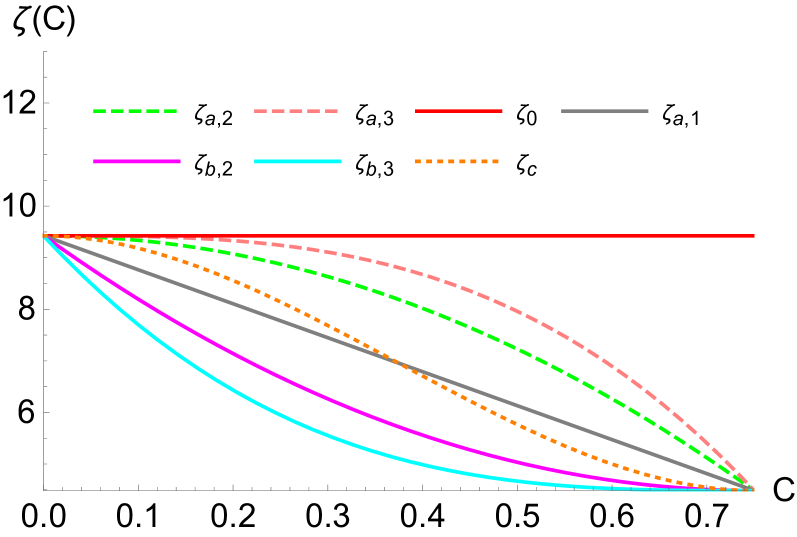
Figure 1: Different functional forms for $\zeta(C)$ function interpolating between the results at $C=0$ and $C=3/4$.

The $\zeta_{0}$ choice corresponds to using a constant shift, i.e. the standard approach for earlier studies. For both $\zeta_{a,n}$ and $\zeta_{b,n}$, using $n=1$ corresponds to a linear interpolation between the $\zeta(0)$ and $\zeta(3/4)$ values. For larger $n$, $\zeta_{a,n}$ is flat close to $C=0$, while $\zeta_{b,n}$ is flat close to $C=3/4$. Finally $\zeta_{c}$ is flat near both $C=0$ and $C=3/4$. We stress that the variations in Eqs. (21) are not normally taken into account when estimating hadronisation with analytic models, which effectively all assume the $\zeta_{0}$ model, corresponding to a constant shift across the whole differential distribution. In Section 4 we will see what impact this has on fits for the strong coupling from experimental data.

In order to gain some insight on how $\zeta(C)$ depends on the recoil scheme, in Appendix B we carry out a fixed-order calculation of this quantity within different schemes to distribute the recoil due to the emission of the gluer among the remaining three partons. In reality, however, the behaviour that we find at fixed order in Appendix B can be substantially modified by the emission of multiple perturbative radiation (as also discussed in Appendix B). Therefore we do not rely on these calculations to assess the impact of $\zeta(C)$ on the fits, but rather use them as an insightful picture of how the leading non-perturbative correction scales across the spectrum of the event shape. We do however note that the concrete recoil schemes all yield shapes that fall below the $\zeta_{a,1}\equiv\zeta_{b,1}$ line.

4 Fit of $\alpha_{s}$ and hadronisation uncertainties

To test how our results affect the extraction of $\alpha_{s}$, we perform a simultaneous fit of the strong coupling and of the non-perturbative parameter $\alpha_{0}(\mu_{I}^{2})$, using data at different centre-of-mass energies from the ALEPH Heister:2003aj and JADE MovillaFernandez:1998ys experiments, as summarised in Table 1. This dataset is smaller than that considered for a similar fit in Ref. Hoang:2015hka , but is largely sufficient for determining how the $\alpha_{s}$ fit result depends on $\zeta(C)$.

Exp.	Q (GeV)	Fit range	N. bins	Ref.
ALEPH	91.2	$0.27<C<0.69$	22	Heister:2003aj
ALEPH	133.0	$0.20<C<0.675$	6	Heister:2003aj
ALEPH	161.0	$0.16<C<0.675$	7	Heister:2003aj
ALEPH	172.0	$0.16<C<0.675$	7	Heister:2003aj
ALEPH	183.0	$0.16<C<0.675$	7	Heister:2003aj
ALEPH	189.0	$0.16<C<0.675$	7	Heister:2003aj
ALEPH	200.0	$0.125<C<0.675$	8	Heister:2003aj
ALEPH	206.0	$0.125<C<0.675$	8	Heister:2003aj
JADE	44.0	$0.61<C<0.68$	2	MovillaFernandez:1998ys

Table 1: Data set considered for the simultaneous $\chi^{2}$ fit of $\alpha_{s}$ and $\alpha_{0}$.

The theory predictions are obtained using 50 bins in the $0\leq C\leq 1$ range, subsequently interpolated in order to be evaluated in correspondence to the experimental data bins. The fit is performed by minimising the $\chi^{2}$ function defined as

$$\chi^{2}= \sum_{i,j}\left(\left.\frac{1}{\sigma}\frac{\hbox{d}\sigma}{\hbox{d}C}(C_{i})\right|^{\rm data}-\left.\frac{1}{\sigma}\frac{\hbox{d}\sigma}{\hbox{d}C}(C_{i})\right|^{\rm th}\right)V^{-1}_{ij}$$

$$\times\left(\left.\frac{1}{\sigma}\frac{\hbox{d}\sigma}{\hbox{d}C}(C_{j})\right|^{\rm data}-\left.\frac{1}{\sigma}\frac{\hbox{d}\sigma}{\hbox{d}C}(C_{j})\right|^{\rm th}\right)\,,$$ (22)

where $V_{ij}$ is the covariance matrix that encodes the correlation between the bins $C_{i}$ and $C_{j}$. The general form of the covariance matrix is $V_{ij}=S_{ij}+E_{ij}$, where $S_{ij}=\delta\sigma_{{\rm stat},\,i}^{2}\delta_{ij}$ is the diagonal matrix of the (uncorrelated) statistical errors in the experimental differential distribution, while $E_{ij}$ contains the experimental systematic covariances. The diagonal entries of $E_{ii}=\delta\sigma_{{\rm syst},i}^{2}$ are given by the experimental systematic uncertainty on the $i$-th bin. For the off-diagonal elements, which are not publicly available, a common choice (used also in Refs. Abbate:2010xh ; Gehrmann:2012sc ; Hoang:2015hka ) is to consider a minimal-overlap model, which defines $E_{ij}$ as

$$E_{ij}={\rm min}\left(\delta\sigma_{{\rm syst},i}^{2},\delta\sigma_{{\rm syst},j}^{2}\right).$$ (23)

For ease of comparison, we adopt the same choice, though we note that for the normalised distributions that we fit here, the true covariance matrix would also include some degree of anti-correlation. The $\chi^{2}$ minimisation is carried out with the TMinuit routine distributed with ROOT and the whole analysis was implemented in the C++ code used for a similar fit in Ref. Gehrmann:2012sc . Results with a diagonal covariance matrix, i.e. without any correlations, are given in Appendix C. They yield almost identical central results for $\alpha_{s}$ and $\alpha_{0}$, smaller $\chi^{2}$ values, and an increase in the experimental errors of ${\cal O}(10\%-20\%)$, which however remain small compared to theoretical uncertainties.

In order to estimate the theoretical uncertainties, we perform the following variations:

• the renormalisation scale $\mu_{R}$ is randomly varied in the range $Q/2\leq\mu_{R}\leq 2\,Q$, while the infrared scale $\mu_{I}$ is set to $2$ GeV;

• for $\mu_{R}=Q$, the resummation scale fraction $x_{C}$ defined in Appendix D (default value $x_{C}=1/2$) is randomly varied by a factor $3/2$ in either direction, namely in the range $1/3\leq x_{C}\leq 3/4$, following the prescription of Ref. Jones:2003yv ;

• for $\mu_{R}=Q$ and $x_{C}=1/2$, the Milan factor $\mathcal{M}$ is randomly varied within $20\%$ of its central value Dokshitzer:1997iz (${\cal M}\simeq 1.49$) to account for non-inclusive effects in the $\langle\delta C\rangle$ shift (2) beyond ${\cal O}(\alpha_{s}^{2})$;

• keeping all of the above parameters at their central values, the parameter $p$ in the modified logarithm defined in Eq. (41) of Appendix D (default value $p=6$) is replaced by $p=5$ and $p=7$. This choice for $p$ is discussed in Appendix D.

The theory error is defined as the envelope of all the above variations. When we quote overall results below, we add the theoretical and experimental errors in quadrature.

We test several models for $\zeta(C)$ as given in Eq. (21) and shown in Fig. 1. Specifically, we consider the constant $\zeta_{0}$ choice, the $\zeta_{a,n}$ model for $n=1,2,3$, the $\zeta_{b,n}$ model for $n=1,2,3$, and the $\zeta_{c}$ model (recall $\zeta_{a,1}\equiv\zeta_{b,1}$).

The results of the fits are given in Fig. 2 and Table 2. Fig. 2 shows results for $\alpha_{s}$ and $\alpha_{0}$: the points give the central result for each $\zeta(C)$ choice, while the corresponding shaded areas represent the envelope of results obtained varying scales and parameters in the theoretical calculation, i.e. our overall theoretical uncertainty. Each point is accompanied by the $\Delta\chi^{2}=1$ ellipse, whose projection along each of the axes defines the $1\,\sigma$ experimental uncertainty. Table 2 provides the numerical values of the central results and overall errors for each $\zeta(C)$ choice, and additionally includes the $\chi^{2}$ result from the fit, Eq. (4), divided by the number of degrees of freedom.

Model	$\alpha_{s}(M_{Z}^{2})$	$\alpha_{0}(\mu_{I}^{2})$	$\chi^{2}/{\rm d.o.f.}$
$\zeta_{0}$	$0.1121\pm 0.0006^{+0.0023}_{-0.0014}$	$0.53\pm 0.01^{+0.07}_{-0.04}$	$1.076$
$\zeta_{a,1}\equiv\zeta_{b,1}$	$0.1142\pm 0.0005^{+0.0026}_{-0.0015}$	$0.52\pm 0.01^{+0.06}_{-0.04}$	$1.045$
$\zeta_{a,2}$	$0.1121\pm 0.0006^{+0.0024}_{-0.0015}$	$0.52\pm 0.01^{+0.07}_{-0.04}$	$1.033$
$\zeta_{a,3}$	$0.1099\pm 0.0007^{+0.0022}_{-0.0014}$	$0.54\pm 0.01^{+0.07}_{-0.05}$	$1.116$
$\zeta_{b,2}$	$0.1163\pm 0.0005^{+0.0028}_{-0.0017}$	$0.51\pm 0.01^{+0.06}_{-0.04}$	$1.079$
$\zeta_{b,3}$	$0.1167\pm 0.0004^{+0.0028}_{-0.0018}$	$0.53\pm 0.01^{+0.06}_{-0.04}$	$1.143$
$\zeta_{c}$	$0.1156\pm 0.0005^{+0.0027}_{-0.0016}$	$0.48\pm 0.01^{+0.05}_{-0.03}$	$1.074$

Table 2: Results of fits for $\alpha_{s}$ and $\alpha_{0}$ using the different functional forms for $\zeta(C)$ reported in Eq. (21). The quoted uncertainties encode the total (statistical and systematic) experimental uncertainty (first number) and the total theoretical uncertainty (second number) estimated as described in the text. The $\chi^{2}$ values are those obtained with central scales and setup. The results have been obtained with the minimum overlap model, Eq. (23), for correlations between experimental systematic uncertainties.

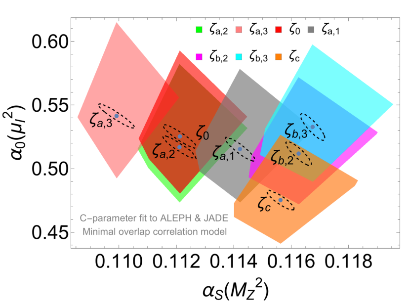
Figure 2: Fit results for $\alpha_{s}$ and $\alpha_{0}$ for different models of $\zeta(C)$. The points indicate the fit corresponding to the central setup of scales and parameters for a given model. The ellipses show the $\Delta\chi^{2}=1$ contours associated with the experimental uncertainty. The shaded areas represent the theory uncertainties due to the variation of additional theoretical parameters as described in the text.

The results with the $\zeta_{0}$ model correspond to the standard implementation of the leading non-perturbative correction, which is assumed to amount to a constant shift across the whole $C$ spectrum. The fit returns

$$\zeta_{0}:~{}~{}\alpha_{s}(M_{Z}^{2})=0.1121^{+0.0024}_{-0.0016}\,,\quad\alpha_{0}(\mu_{I}^{2})=0.53^{+0.07}_{-0.05}\,,$$

and agrees well with that of Ref. Hoang:2015hka , albeit with larger uncertainties, in part due to our use of NNLL+NNLO rather than N³LL+NNLO theory predictions. We observe that several models lead to a $\chi^{2}$ value that is the same as, or smaller than, that for the $\zeta_{0}$ shape. In particular, the $\zeta_{b,2}$ model returns

$$\zeta_{b,2}:~{}~{}\alpha_{s}(M_{Z}^{2})=0.1163^{+0.0028}_{-0.0018}\,,\quad\alpha_{0}(\mu_{I}^{2})=0.51^{+0.06}_{-0.04}\,,$$

with a $\chi^{2}$ that is similar to that of the $\zeta_{0}$ fit. This corresponds to an increase in $\alpha_{s}(M_{Z}^{2})$ of about $3.7\%$. In a number of models ($\zeta_{a,1}\equiv\zeta_{b,1}$, $\zeta_{b,2}$, $\zeta_{b,3}$, and $\zeta_{c}$) the values of $\alpha_{s}$ become compatible with the world average PDGQCD2019 $\alpha_{s}^{\rm W.A.}=0.1179\pm 0.0010$. The result with the smallest $\chi^{2}$ is the $\zeta_{a,2}$ model, which yields a rather small value of $\alpha_{s}=0.1121^{+0.0024}_{-0.0016}$. However the investigations of Appendix B, with a variety of concrete recoil-scheme prescriptions, seem to disfavour the $\zeta_{a,2}$ shape, suggesting that yet other factors may be relevant for maximising the fit quality.

Overall, the results suggest that one should allow for a $3{-}4\%$ uncertainty in $\alpha_{s}$ extractions from $e^{+}e^{-}$ $C$-parameter data, associated with limitations in our current ability to estimate hadronisation corrections.

5 Conclusions

In this letter we have pointed out that the presence of a Sudakov shoulder in the differential distribution of some event-shape observables, such as the $C$ parameter, can be exploited to gain insight on the observable dependence of the leading ($\sim 1/Q$) hadronisation correction to the spectrum. We found that the leading hadronisation correction at the Sudakov shoulder ($C=3/4$) is over a factor of two smaller than the corresponding value in the two-jet ($C=0$) limit.

In order to assess the impact of this observation on the fit of the strong coupling constant, we performed a set of fits using different assumptions on the scaling of the non-perturbative correction between the two points.

Our study is by no means exhaustive, and the inclusion of additional physical effects (such as the impact of bottom-mass effects) as well as a careful assessment of other sources of systematic uncertainty (such as the dependence on the fit range and the choice of correlation model) is necessary. However, it clearly reveals that current uncertainties in the modelling of hadronisation corrections can arguably impact the extractions of the strong coupling from event shapes at the several percent level. In particular, some of the models tested here lead to an increase in the extracted value of the strong coupling by $3\%-4\%$, which then becomes compatible with the world average to within uncertainties.

This necessarily raises the question of whether such observables should still be adopted for percent-accurate determinations of the strong coupling at LEP energies. Similar considerations may apply to extractions of $\alpha_{s}$ obtained with jet observables, for instance those relying on accurate calculations for jet rates GehrmannDeRidder:2008ug ; Weinzierl:2008iv ; Weinzierl:2009ms ; DelDuca:2016ily ; Banfi:2016zlc (e.g. the fits of Refs. Dissertori:2009qa ; Verbytskyi:2019zhh ) or modifications of $e^{+}e^{-}$ event shapes by means of grooming techniques Frye:2016aiz ; Baron:2018nfz ; Kardos:2018kth (an example being the analysis of Ref. Marzani:2019evv ). Further studies are certainly warranted to investigate whether it is possible to better understand hadronisation for such observables across their whole spectrum, for example exploiting the large-$n_{f}$ calculational methods of Ref. FerrarioRavasio:2018ubr .

Appendix A Some relevant quantities

In the present section we report the expressions for the anomalous dimensions used in the main text. The QCD $\beta$ function is defined by the renormalisation group equation for the QCD coupling constant

$$\frac{\hbox{d}\alpha_{s}(\mu)}{\hbox{d}\ln\mu^{2}}=-\alpha_{s}(\mu)\bigg{(}\frac{\alpha_{s}(\mu)}{\pi}\beta_{0}+\frac{\alpha_{s}^{2}(\mu)}{\pi^{2}}\beta_{1}+\ldots\bigg{)},$$ (24)

where the first two coefficients read

$$\beta_{0}= \frac{11}{12}C_{A}-\frac{1}{3}T_{F}n_{F},$$

$$\beta_{1}= \frac{17}{24}C_{A}^{2}-\frac{5}{12}C_{A}T_{F}n_{F}-\frac{1}{4}C_{F}T_{F}n_{F}.$$ (25)

The $K^{(i)}$ coefficients that appear in the non-perturbative shift (2) arise from the perturbative relation between the strong coupling in the soft physical scheme Catani:1990rr ; Banfi:2018mcq ; Catani:2019rvy , denoted here by $\tilde{\alpha}_{s}$, and the $\overline{\rm MS}$ coupling $\alpha_{s}\equiv\alpha_{s}(\mu^{2})$

$$\tilde{\alpha}_{s}(\mu^{2})=\alpha_{s}\left(1+\frac{\alpha_{s}}{2\pi}K^{(1)}+\left(\frac{\alpha_{s}}{2\pi}\right)^{2}K^{(2)}+{\cal O}(\alpha_{s}^{3})\right)\,.$$ (26)

They read Catani:1990rr ; Banfi:2018mcq ; Catani:2019rvy

$$K^{(1)} =C_{A}\left(\frac{67}{18}-\frac{\pi^{2}}{6}\right)-\frac{5}{9}n_{f}\,,$$ (27a)

$$K^{(2)} =C_{A}^{2}\left(\frac{245}{24}-\frac{67}{9}\zeta_{2}+\frac{11}{6}\zeta_{3}+\frac{11}{5}\zeta_{2}^{2}\right)$$

$$+C_{F}n_{f}\left(-\frac{55}{24}+2\zeta_{3}\right)$$

$$+C_{A}n_{f}\left(-\frac{209}{108}+\frac{10}{9}\zeta_{2}-\frac{7}{3}\zeta_{3}\right)-\frac{1}{27}n_{f}^{2}$$

$$+\frac{\beta_{0}}{2}\left(C_{A}\left(\frac{808}{27}-28\zeta_{3}\right)-\frac{224}{54}n_{f}\right)\,.$$ (27b)

Appendix B Fixed-order prediction for $\zeta(C)$ and recoil scheme dependence

It is instructive to repeat the calculation (10) starting from a generic $q\bar{q}g$ configuration in the region $0\!<\!C\!<\!3/4$. In this case the value of $\Delta C$ in Eq. (9) will depend on the specific scheme used to distribute the recoil due to the emission of the gluer among the remaining three partons. Therefore, the definition of $\zeta(C)$ away from the singular points at $C=0$ and $C=3/4$ must be modified as follows

$$\zeta(C)= \frac{1}{\cal N}\lim_{\epsilon\to 0}\frac{\pi Q}{2\alpha_{s}C_{F}}\int d\Phi_{q\bar{q}g}\,[dk]\,M_{q\bar{q}g}^{2}(\{p_{i}\})\,M^{2}(k)$$

$$\times \Delta C(\{p^{\prime}_{i}\},\{p_{i}\};k)\delta\left(C-C(\{p_{i}\})\right)\,\delta(k_{t}-\epsilon)\,,$$ (28)

with the normalisation $\cal{N}$ given by

$${\cal N}=\int d\Phi_{q\bar{q}g}\,M_{q\bar{q}g}^{2}(\{p_{i}\})\,\delta\left(C-C(\{p_{i}\})\right)\,.$$ (29)

In the above two equations $\Phi_{q\bar{q}g}$ denotes the phase space of the $q\bar{q}g$ system and $M_{q\bar{q}g}^{2}(\{p_{i}\})$ is the corresponding squared amplitude evaluated with the unrecoiled momenta $\{p_{i}\}=\{p_{q},p_{\bar{q}},p_{g}\}$ prior to the emission of the gluer $k$. We see that as we approach one of the singular points $\Delta C(\{p^{\prime}_{i}\},\{p_{i}\};k)\simeq\Delta C(k)$ and we reproduce Eq. (10). Away from those points, the recoil will induce a linear dependence on the gluer’s momentum, hence affecting the value of $\zeta(C)$ in a way that potentially depends on the specific model of recoil. The fixed-order calculation of Eq. (B) will provide some level of insight into how the leading non-perturbative correction varies across the spectrum of the event shape.

For an emission off a given dipole $\{ij\}$ ($\{qg\}$, $\{q\bar{q}\}$ or $\{\bar{q}g\}$), we express the gluer’s momentum $k$ by means of the Sudakov parametrisation

$$k=\alpha_{k}p_{i}+\beta_{k}p_{j}+k_{\perp}\,,$$ (30)

where $\alpha_{k}=(p_{j}\cdot k)/(p_{i}\cdot p_{j})$, $\beta_{k}=(p_{i}\cdot k)/(p_{i}\cdot p_{j})$, and $k_{\perp}=k_{t}\left[{n}_{\perp,1}\cos\phi+{n}_{\perp,2}\sin\phi\right]$, with ${n}_{\perp,m}^{2}=-1$, ${n}_{\perp,m}\cdot p_{i/j}=0$ ($m=1,2$), ${n}_{\perp,1}\cdot{n}_{\perp,2}=0$. We consider the following four recoil schemes

1. CS Dipole: the scheme is inspired by the Catani-Seymour map Catani:1996vz . For an emission $k$ off a dipole $\{ij\}$ one identifies the emitter and spectator by considering the following quantity

   $$y_{\ell k}=(p_{\ell}\cdot k)/E_{\ell}\,,$$ (31)

   computed in the event centre-of-mass frame with $\ell=i,j$. The emitter is then the dipole end corresponding to the smaller $y_{\ell k}$. Once the emitter (say $p_{i}$) and the spectator ($p_{j}$) are identified, the recoil is distributed as follows

   $$p^{\prime}_{i} =p_{i}-k+\frac{(k\cdot p_{i})}{(p_{i}\cdot p_{j})-(k\cdot p_{j})}p_{j}\,,$$

   $$p^{\prime}_{j} =\left(1-\frac{(k\cdot p_{i})}{(p_{i}\cdot p_{j})-(k\cdot p_{j})}\right)p_{j}\,.$$ (32)

   We also examined an alternative scheme in which the distance $y_{\ell k}$ is computed in the dipole centre-of-mass frame. The two schemes produce identical results for the calculation considered in this appendix, and therefore we omit further discussion of the latter variant.

2. PanLocal Dasgupta:2020fwr (antenna variant): the recoil is shared locally within the dipole ends as

   $$p^{\prime}_{i} =\alpha_{i}p_{i}+\beta_{i}p_{j}-fk_{\perp}\,,$$

   $$p^{\prime}_{j} =\alpha_{j}p_{i}+\beta_{j}p_{j}-(1-f)k_{\perp}\,.$$ (33)

   The quantities $\alpha_{i/j}$ and $\beta_{i/j}$ in Eq. (2) are fully specified by the requirements $(p^{\prime})^{2}_{i/j}=0$, $(p^{\prime}_{i}+p^{\prime}_{j}+k)=(p_{i}+p_{j})$ and $p^{\prime}_{i}=p_{i}$ for $k_{t}\to 0$. The PanLocal Dasgupta:2020fwr rapidity-like variable $\bar{\eta}$ is defined as

   $$\bar{\eta}=\ln\left(\frac{\alpha_{k}}{k_{t}}\sqrt{\frac{s_{i}s_{ij}}{s_{j}}}\right)\,,$$ (34)

   where $s_{ij}=2p_{i}\cdot p_{j}$, $s_{i}=2p_{i}\cdot Q$, and $Q$ is the total event momentum. In the event centre-of-mass frame, $\bar{\eta}=0$ corresponds to a direction equidistant in angle from $p_{i}$ and $p_{j}$. The function $f$ is responsible for sharing the transverse recoil among $p_{i}$ and $p_{j}$ and it is defined as

   $$f\equiv f(\bar{\eta})=\frac{e^{2\bar{\eta}}}{1+e^{2\bar{\eta}}}\,.$$ (35)

   Finally, we have

   $$\alpha_{i} =\frac{(\sqrt{\lambda_{1}}+\sqrt{\lambda_{2}})^{2}+4f^{2}}{4(1-\beta_{k})}\,\alpha_{k}\beta_{k}\,,$$

   $$\beta_{i} =\frac{(\sqrt{\lambda_{1}}-\sqrt{\lambda_{2}})^{2}+4f^{2}}{4(1-\alpha_{k})}\,\alpha_{k}\beta_{k}\,,$$

   $$\alpha_{j} =\frac{(\sqrt{\lambda_{1}}-\sqrt{\lambda_{2}})^{2}+4(1-f)^{2}}{4(1-\beta_{k})}\,\alpha_{k}\beta_{k}\,,$$

   $$\beta_{j} =\frac{(\sqrt{\lambda_{1}}+\sqrt{\lambda_{2}})^{2}+4(1-f)^{2}}{4(1-\alpha_{k})}\,\alpha_{k}\beta_{k}\,,$$ (36)

   with

   $$\lambda_{1} =(1-\alpha_{k}-\beta_{k})/(\alpha_{k}\beta_{k})\,,$$

   $$\lambda_{2} =\lambda_{1}+4f(1-f)\,.$$ (37)

3. PanGlobal Dasgupta:2020fwr : the longitudinal recoil is assigned locally within the dipole as

   $$\bar{p}_{i} =(1-\alpha_{k})p_{i}\,,$$

   $$\bar{p}_{j} =(1-\beta_{k})p_{j}\,,$$ (38)

   and the transverse recoil is assigned by applying a Lorentz boost and a rescaling to the full event so as to obtain final momenta $\{p^{\prime},k^{\prime}\}$ whose sum gives the original total momentum $Q$ (see Dasgupta:2020fwr for details).
   

4. FHP: the scheme is inspired by that proposed by Forshaw-Holguin-Plätzer in Ref. Forshaw:2020wrq . It is similar to PanGlobal, with the difference that only the longitudinal recoil along the emitter, say $p_{i}$, is assigned locally

   $$\bar{p}_{i} =(1-\alpha_{k})p_{i}\,,$$ (39)

   and the remaining longitudinal and transverse recoil is assigned by applying a Lorentz boost and a rescaling to the full event as in the PanGlobal scheme. Unlike the proposal in the original paper Forshaw:2020wrq , we identify the emitter $p_{i}$ with the dipole end closer in angle to $k$ in the event centre-of-mass frame, that is the one with the smaller $y_{\ell k}$ defined in Eq. (31). For our purposes, this is physically similar to what is done in Ref. Forshaw:2020wrq .

The results of the computation are reported in Figure 3, where for comparison we also report the curves corresponding to the profiles $\zeta_{a,1}\equiv\zeta_{b,1}$, $\zeta_{a,2}$ and $\zeta_{b,2}$. We observe that the CS Dipole, PanLocal and PanGlobal schemes yield nearly identical results for $\zeta(C)$, which depart very sharply from the asymptotic value in the two-jet limit and approach the shape of the $\zeta_{b}$-type profiles at large values of $C$. Instead, the FHP scheme gives a less convex shape, close to a linear scaling in the fit region (indicated by the unshaded area in the plot).

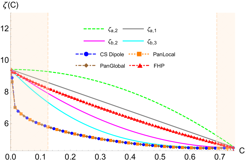
Figure 3: Fixed order calculation of $\zeta(C)$ within different recoil schemes, compared to the analytic profiles given in the main text. The unshaded area indicates the typical $C$ region where the fit of $\alpha_{s}$ is performed. The CS Dipole, PanLocal and PanGlobal results coincide.

We believe that the similarity between the CS Dipole, PanLocal and PanGlobal schemes originates from the fact that, in the presence of a single perturbative gluon, $\zeta(C)$ is largely insensitive to the precise distribution of the transverse recoil among the particles in the event, which at this order and for this particular observable, is washed out by the integration over the azimuth and rapidity of the perturbative gluon $p_{g}$. Conversely, the result does seem to depend on how the longitudinal recoil is assigned. The CS Dipole, PanLocal and PanGlobal schemes schemes all assign the longitudinal recoil locally within the emitting dipole, while in the FHP scheme part of the longitudinal recoil is shared among all particles in the event.

Note that all recoil schemes appear to be below the $\zeta_{a,1}\equiv\zeta_{b,1}$ model. This tends to disfavour the $\zeta_{a,2}$ type model for interpolation of $\zeta(C)$ between $C=0$ and $C=3/4$, even though it gave the lowest $\chi^{2}$ in the $\alpha_{s}$ fits in Section 4.

A final comment concerns the limitations of the fixed-order nature of the study carried out in this appendix. At the order at which we work, the fact that we force the perturbative $q\bar{q}g$ system to have a given value of the $C$-parameter causes the perturbative gluon to have a hardness comparable to $CQ$. Were we to go to higher orders, it would become possible for the perturbative event to contain additional, much softer gluons. Those gluons could also be involved in the recoil from the non-perturbative gluer, further altering the gluer’s impact on the $C$-parameter. To take this into account, one would need to carry out a non-global type resummation that includes any number of perturbative soft gluons between the momentum scale set by the $C$-parameter value and the non-perturbative scale. First investigations in this direction (with just the PanGlobal recoil for the gluer) suggest that the impact of the resummation is non-negligible, and also continue to favour $\zeta(C)$ profiles that are below the linear $\zeta_{a,1}\equiv\zeta_{b,1}$ profile.

Appendix C Fits with uncorrelated systematic experimental uncertainties

In this appendix we report the simultaneous fit of $\alpha_{s}$ and $\alpha_{0}$ obtained with the same procedure outlined in the main text, albeit replacing the model (23) with the simpler assumption of uncorrelated systematic uncertainties in the experimental data, namely

$$E_{ij}=\delta\sigma_{{\rm syst},i}^{2}\,\delta_{ij}\,.$$ (40)

The results are given in Table 3. Relative to Table 2, the absence of correlations leads to an increase in the experimental uncertainties for $\alpha_{s}$ of ${\cal O}(10\%-20\%)$, and the $\chi^{2}$ values decrease. The central $\alpha_{s}$ and $\alpha_{0}$ results are essentially unchanged, as are the theory systematics.

Model	$\alpha_{s}(M_{Z}^{2})$	$\alpha_{0}(\mu_{I}^{2})$	$\chi^{2}/{\rm d.o.f.}$
$\zeta_{0}$	$0.1122\pm 0.0007^{+0.0024}_{-0.0014}$	$0.52\pm 0.01^{+0.07}_{-0.04}$	$0.813$
$\zeta_{a,1}\equiv\zeta_{b,1}$	$0.1142\pm 0.0006^{+0.0026}_{-0.0015}$	$0.52\pm 0.01^{+0.06}_{-0.04}$	$0.796$
$\zeta_{a,2}$	$0.1121\pm 0.0007^{+0.0024}_{-0.0015}$	$0.52\pm 0.01^{+0.07}_{-0.04}$	$0.787$
$\zeta_{a,3}$	$0.1100\pm 0.0008^{+0.0022}_{-0.0014}$	$0.54\pm 0.01^{+0.07}_{-0.05}$	$0.845$
$\zeta_{b,2}$	$0.1162\pm 0.0005^{+0.0028}_{-0.0017}$	$0.51\pm 0.01^{+0.06}_{-0.04}$	$0.822$
$\zeta_{b,3}$	$0.1167\pm 0.0005^{+0.0028}_{-0.0018}$	$0.53\pm 0.01^{+0.06}_{-0.04}$	$0.870$
$\zeta_{c}$	$0.1156\pm 0.0006^{+0.0027}_{-0.0016}$	$0.48\pm 0.01^{+0.05}_{-0.03}$	$0.807$

Table 3: Results of fits for $\alpha_{s}$ and $\alpha_{0}$ using the different functional forms for $\zeta(C)$, as in Table 2, but with an assumption of uncorrelated experimental uncertainties instead of the minimum overlap model.

Appendix D Modified logarithms and comparison to profile functions

In order to properly ensure that the resummation is turned off at the kinematic endpoint of the differential distribution, we modify the resummed logarithms by making the replacement

$$\ln\frac{6\,x_{C}}{C}\to L\equiv\frac{1}{p}\ln\left(1+\frac{\left(6\,x_{C}\right)^{p}}{C^{p}}-\frac{\left(6x_{C}\right)^{p}}{C_{\rm max}^{p}}\right)\,,$$ (41)

where $p$ denotes a positive parameter, and $C_{\rm max}$ is the kinematic endpoint of the $C$-parameter distribution in the multi-jet regime, i.e. $C_{\rm max}=1$. The prescription of Eq. (41) is but a possible choice and other sensible solutions can be found in the literature (see e.g. Ref. Hoang:2015hka ). This ambiguity introduces an additional theoretical uncertainty in the calculation that must be carefully estimated. The quantity $x_{C}$ is of order one and its variation estimates the resummation uncertainty due to missing higher-logarithmic corrections. Specifically, the $\Sigma^{\rm N^{k}LL}(C)$ resummed cross section acquires a net $x_{C}$ dependence such that,

$$\frac{d\Sigma^{\rm N^{k}LL}(C)}{d\ln x_{C}}={\cal O}(\rm{N^{k+1}LL})\,,$$ (42)

in the logarithmic limit as $C\to 0$. Similarly, the parameter $p$ determines how quickly the resummation is turned off in the region $C\sim C_{\rm max}$.

The choice of $p$ must guarantee that the resummation does not substantially affect the prediction in regions of the spectrum dominated by hard radiation. An inspection of the first-order $C$-parameter distribution reveals contributions suppressed by a (linear) power of $C$ relative to the dominant $(\ln C)/C$ dependence. Were we to take $p=1$, the first-order expansion of the resummation would be associated with perturbative linear power-suppressed contributions whose coefficient would be larger than that observed in the exact fixed-order calculation. Accordingly, we believe it is sensible to apply the restriction $p>1$ to avoid such contributions, and ensure that the resummation does not affect the dominant scaling at subleading power. With this constraint, we find that the extracted value of $\alpha_{s}$ depends only very mildly on the choice of $p$ and well within the quoted theoretical uncertainties. We then choose $p=6$ and $x_{C}=1/2$ and vary both parameters as outlined in Section 4 in the uncertainty estimate. This specific choice is motivated by the fact that the scaling of the modified logarithm (41) in most of the fit range that we adopted in Section 4 happens to reproduce that of the profiled logarithms of the soft function of Ref. Hoang:2015hka , which we use as a reference benchmark in our study. A comparison between the two prescriptions is shown in Figure 4

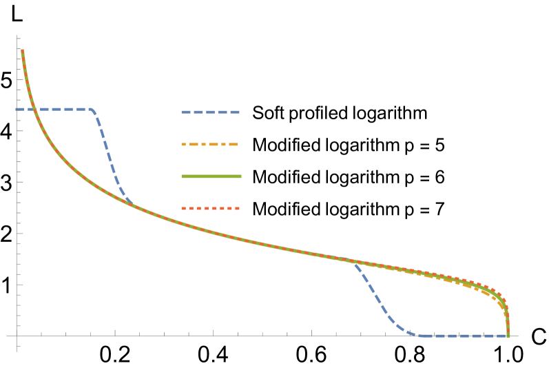
Figure 4: The figure displays a comparison between the resummed modified logarithm (41) with different $p$ values and the profiled logarithm $\ln(Q/\mu_{s}(C))$ where the profiled soft scale $\mu_{s}(C)$ is defined in Ref. Hoang:2015hka . The centre-of-mass energy $Q$ is set to the $Z$-boson mass.

References

- (1) M. Tanabashi, et al., Phys. Rev. D98(3), 030001 (2018)
- (2) J. Huston, K. Rabbertz, G. Zanderighi. 2019 update to the quantum Chromodynamics review (2019). URL http://pdg.lbl.gov/2019/reviews/rpp2019-rev-qcd.pdf
- (3) R. Keith Ellis, G. Zanderighi, in From My Vast Repertoire …: Guido Altarelli’s Legacy, ed. by A. Levy, S. Forte, G. Ridolfi (World Scientific, Singapore, 2019), pp. 31–52
- (4) R. Abbate et al., Phys.Rev. D83, 074021 (2011), 1006.3080
- (5) A. Hoang et al., Phys. Rev. D91(9), 094018 (2015), 1501.04111
- (6) P. Zyla, et al., PTEP 2020(8), 083C01 (2020)
- (7) M. Bruno, M. Dalla Brida, P. Fritzsch, T. Korzec, A. Ramos, S. Schaefer, H. Simma, S. Sint, R. Sommer, Phys. Rev. Lett. 119(10), 102001 (2017), 1706.03821
- (8) A. Verbytskyi, A. Banfi, A. Kardos, P.F. Monni, S. Kluth, G. Somogyi, Z. Szőr, Z. Trócsányi, Z. Tulipánt, G. Zanderighi, JHEP 08, 129 (2019), 1902.08158
- (9) R.W.L. Jones, M. Ford, G.P. Salam, H. Stenzel, D. Wicke, JHEP 12, 007 (2003), hep-ph/0312016
- (10) G. Dissertori et al., JHEP 02, 040 (2008), 0712.0327
- (11) S. Bethke, S. Kluth, C. Pahl, J. Schieck, Eur. Phys. J. C64, 351 (2009), 0810.1389
- (12) T. Becher, M. Schwartz, JHEP 07, 034 (2008), 0803.0342
- (13) R.A. Davison, B.R. Webber, Eur. Phys. J. C59, 13 (2009), 0809.3326
- (14) G. Dissertori, A. Gehrmann-De Ridder, T. Gehrmann, E.W.N. Glover, G. Heinrich, G. Luisoni, H. Stenzel, JHEP 08, 036 (2009), 0906.3436
- (15) T. Gehrmann, M. Jaquier, G. Luisoni, Eur. Phys. J. C67, 57 (2010), 0911.2422
- (16) Y.T. Chien, M.D. Schwartz, JHEP 08, 058 (2010), 1005.1644
- (17) G. Abbiendi et al., Eur. Phys. J. C71, 1733 (2011), 1101.1470
- (18) T. Gehrmann, G. Luisoni, P.F. Monni, Eur. Phys. J. C73(1), 2265 (2013), 1210.6945
- (19) R. Abbate, M. Fickinger, A.H. Hoang, V. Mateu, I.W. Stewart, Phys. Rev. D86, 094002 (2012), 1204.5746
- (20) A. Kardos et al., Eur. Phys. J. C78(6), 498 (2018), 1804.09146
- (21) G. Dissertori et al., Phys. Rev. Lett. 104, 072002 (2010), 0910.4283
- (22) J. Schieck, S. Bethke, S. Kluth, C. Pahl, Z. Trocsanyi, Eur. Phys. J. C73(3), 2332 (2013), 1205.3714
- (23) A. Kardos, G. Somogyi, A. Verbytskyi, (2020), 2009.00281
- (24) E. Gardi, L. Magnea, JHEP 08, 030 (2003), hep-ph/0306094
- (25) S. Ferrario Ravasio, P. Nason, C. Oleari, JHEP 01, 203 (2019), 1810.10931
- (26) S. Catani, B.R. Webber, JHEP 10, 005 (1997), hep-ph/9710333
- (27) S. Catani, B.R. Webber, Phys. Lett. B427, 377 (1998), hep-ph/9801350
- (28) R. Ellis, D. Ross, A. Terrano, Nucl. Phys. B 178, 421 (1981)
- (29) G. Parisi, Phys. Lett. 74B, 65 (1978)
- (30) J.F. Donoghue, F.E. Low, S.Y. Pi, Phys. Rev. D20, 2759 (1979)
- (31) A. Gehrmann-De Ridder et al., JHEP 12, 094 (2007), 0711.4711
- (32) S. Weinzierl, JHEP 06, 041 (2009), 0904.1077
- (33) V. Del Duca et al., Phys. Rev. Lett. 117(15), 152004 (2016), 1603.08927
- (34) S.G. Gorishnii, A.L. Kataev and S.A. Larin, Phys. Lett. B259, 144 (1991)
- (35) P. Nason, C. Oleari, Nucl. Phys. B521, 237 (1998), hep-ph/9709360
- (36) A. Denner, S. Dittmaier, T. Gehrmann, C. Kurz, Phys. Lett. B679, 219 (2009), 0906.0372
- (37) A.H. Hoang, D.W. Kolodrubetz, V. Mateu, I.W. Stewart, Phys. Rev. D91(9), 094017 (2015), 1411.6633
- (38) A. Banfi, H. McAslan, P.F. Monni, G. Zanderighi, JHEP 05, 102 (2015), 1412.2126
- (39) S. Catani, L. Trentadue, G. Turnock, B.R. Webber, Nucl. Phys. B407, 3 (1993)
- (40) P.F. Monni, T. Gehrmann, G. Luisoni, JHEP 08, 010 (2011), 1105.4560
- (41) Y.L. Dokshitzer, A. Lucenti, G. Marchesini, G.P. Salam, Nucl. Phys. B511, 396 (1998), hep-ph/9707532. [Erratum: Nucl. Phys.B593,729(2001)]
- (42) M. Dasgupta, L. Magnea, G. Smye, JHEP 11, 025 (1999), hep-ph/9911316
- (43) M. Beneke, V.M. Braun, L. Magnea, Nucl. Phys. B497, 297 (1997), hep-ph/9701309
- (44) Y.L. Dokshitzer, G. Marchesini, B.R. Webber, Nucl. Phys. B469, 93 (1996), hep-ph/9512336
- (45) Y.L. Dokshitzer, B.R. Webber, Phys. Lett. B352, 451 (1995), hep-ph/9504219
- (46) Y.L. Dokshitzer, A. Lucenti, G. Marchesini, G.P. Salam, JHEP 05, 003 (1998), hep-ph/9802381
- (47) A. Banfi, Y.L. Dokshitzer, G. Marchesini, G. Zanderighi, JHEP 05, 040 (2001), hep-ph/0104162
- (48) M. Dasgupta, G.P. Salam, J. Phys. G 30, R143 (2004), hep-ph/0312283
- (49) A. Heister, et al., Eur. Phys. J. C35, 457 (2004)
- (50) P.A. Movilla Fernandez, O. Biebel, S. Bethke, in High-energy physics. Proceedings, 29th International Conference, ICHEP’98, Vancouver, Canada, July 23-29, 1998. Vol. 1, 2 (1998)
- (51) A. Gehrmann-De Ridder et al., Phys. Rev. Lett. 100, 172001 (2008), 0802.0813
- (52) S. Weinzierl, Phys. Rev. Lett. 101, 162001 (2008), 0807.3241
- (53) V. Del Duca et al., Phys. Rev. D94(7), 074019 (2016), 1606.03453
- (54) A. Banfi, H. McAslan, P.F. Monni, G. Zanderighi, Phys. Rev. Lett. 117(17), 172001 (2016), 1607.03111
- (55) C. Frye, A.J. Larkoski, M.D. Schwartz, K. Yan, JHEP 07, 064 (2016), 1603.09338
- (56) J. Baron, S. Marzani, V. Theeuwes, JHEP 08, 105 (2018), 1803.04719. [erratum: JHEP05,056(2019)]
- (57) A. Kardos, G. Somogyi, Z. Trócsányi, Phys. Lett. B786, 313 (2018), 1807.11472
- (58) S. Marzani, D. Reichelt, S. Schumann, G. Soyez, V. Theeuwes, JHEP 11, 179 (2019), 1906.10504
- (59) S. Catani, B.R. Webber, G. Marchesini, Nucl. Phys. B349, 635 (1991)
- (60) A. Banfi, B.K. El-Menoufi, P.F. Monni, JHEP 01, 083 (2019), 1807.11487
- (61) S. Catani, D. De Florian, M. Grazzini, Eur. Phys. J. C79(8), 685 (2019), 1904.10365
- (62) S. Catani, M. Seymour, Nucl. Phys. B 485, 291 (1997), hep-ph/9605323. [Erratum: Nucl.Phys.B 510, 503–504 (1998)]
- (63) M. Dasgupta, F.A. Dreyer, K. Hamilton, P.F. Monni, G.P. Salam, G. Soyez, Phys. Rev. Lett. 125(5), 052002 (2020), 2002.11114
- (64) J.R. Forshaw, J. Holguin, S. Plätzer, JHEP 09, 014 (2020), 2003.06400