0 \SetWatermarkAngle90
Department of Physics and Astronomy \EdefEscapeHextitle.sectiontitle.section\EdefEscapeHexTitlepageTitlepage\hyper@anchorstarttitle.section\hyper@anchorend
Alignment of the straw tracking detectors for the Fermilab Muon experiment and systematic studies for a muon electric dipole moment measurement
Abstract
The Fermilab Muon experiment is currently preparing for its fourth data-taking period (Run-4). The experiment-wide effort on the analysis of Run-1 data is nearing completion, with the announcement of the first result expected in the coming months. The final goal of the experiment is to determine the muon magnetic anomaly, , to a precision of 140 ppb. This level of precision will provide indirect evidence of new physics, if the central value agrees with the previously-measured value of . Essential in reducing the systematic uncertainty on , through measurements of the muon beam profile, are the in-vacuum straw tracking detectors. A crucial prerequisite in obtaining accurate distributions of the beam profile is the internal alignment of the tracking detectors, which is described in this thesis. As a result of this position calibration, the tracking efficiency has increased by , while the track quality increased by .
This thesis also discusses an additional measurement that will be made using the tracking detectors: a search for an electric dipole moment (EDM) of the muon, through the direct detection of an oscillation in the average vertical angle of the from the decay. An observation of a muon EDM would be evidence of new physics and would provide a new source of CP violation in the charged lepton sector. Essential in measuring the EDM, as well as , are accurate and precise estimations of potential non-zero radial and longitudinal magnetic fields, which were estimated using the Run-1 data. In addition, a preliminary analysis using the Run-1 data was undertaken to estimate the available precision for the measurement using the tracking detectors.
abstract.sectionabstract.section\EdefEscapeHexAbstractAbstract\hyper@anchorstartabstract.section\hyper@anchorend
impact.sectionimpact.section\EdefEscapeHexImpact statementImpact statement\hyper@anchorstartimpact.section\hyper@anchorend {impact} The results of the fundamental research increase humanity’s understanding of the Universe and are of great value for society. The Fermilab experiment will make two measurements to establish the presence of new physics – new particles or forces. The work described in this thesis has had a direct contribution in making these measurements possible. Should signs of new physics be observed, it would result in the first fundamental discovery in the field of experimental particle physics since 2012, and would set a clear pathway for future experiments to explore this new potential phenomenon more rigorously.
As has been the case in the past, fundamental discoveries in particle physics were later able to significantly benefit humanity technologically, beyond their original scope of research. For example, proton therapy is now an established procedure to cure cancer, with its origin rooted in particle accelerators. Moreover, an emerging challenge for a truly globalised world of the 21st century is global security. Notably, research into muons allowed for the development of muon tomography, enabling to improve the detection of nuclear materials. It remains to be seen what technological advancements will be enabled by new physics.
The technological expertise developed during this thesis is directly applicable to tackle one of the four Grand Challenges111HM Government, Industrial Strategy White Paper (2017). to put the UK at the forefront of the industries of the future – AI and Data Economy. By 2030, the AI industry is projected to expand the UK economy by 22%222McKinsey Global Institute, Artificial intelligence in the United Kingdom (2019)..
acknowledgements.sectionacknowledgements.section\EdefEscapeHexAcknowledgementsAcknowledgements\hyper@anchorstartacknowledgements.section\hyper@anchorend
Acknowledgements.
First and foremost, I would like to express my deepest gratitude to my supervisor, Mark Lancaster, who, through his outstanding leadership, made my PhD journey a truly remarkable experience. Mark, I greatly value all the advice, support, and encouragement that you have given me over the years – thank you! A special recognition should be given to Rebecca Chislett, Joe Price, and James Mott. I am truly grateful for the help that you have provided in tackling many of the arising challenges in this thesis, and for investing your time in me. Your ability to solve difficult tasks with ease and a friendly approach serves as an inspiration to me. Nicholas Kinnaird and Saskia Charity, I appreciate your time in answering many of my questions on tracking and data analysis, especially when you were busy finishing your own theses. You both have set a tremendous example for me to follow. I would like to thank the members of the tracker group: Brendan Casey, Tammy Walton, Alessandra Luca, and others, for creating a fantastic environment to collaborate and share ideas. Past and present members of the UCL team have also provided ample support and inspiration to me: Tom Stuttard, Gavin Hesketh, Samer Al-Kilani, Matt Warren, Erdem Motuk, and Dominika Vasilkova. Moreover, I would like to thank the entire collaboration: I could never have imagined to have a group of such talented, hard-working, attentive and friendly colleagues is possible – you are all absolutely brilliant! In particular, I would like to thank – for many exciting discussions, interactions and shenanigans – Sam Grant, Sophie Middleton, Sean Foster, Will Turner, Tabitha Halewood-Leagas, Talal Albahri, Meghna Bhattacharya, Sudeshna Ganguly, Jarek Kaspar, Anna Driutti, Chris Polly, Karie Badgley, Mandy Rominsky, and Brendan Kiburg. A big thanks to Leah Welty-Rieger and the \say Tevatron ring-run crew, as well as coach Sonny Ross, at the Prime Muay Thai club. The intense exercise provided a welcome distraction from the never-ending data analysis. I would also like to thank Tania Claudette, at the Fermilab’s Frontier Pub, for the endless supply of IPAs and for playing the Black Keys on demand! Finally, I would like to thank my parents for their endless support, love, and understanding. It would not have been possible to get here without you, and I am truly fortunate to have you in my life.toc.sectiontoc.section\EdefEscapeHexContentsContents\hyper@anchorstarttoc.section\hyper@anchorend
List of acronyms
- ASDQ
- amplified shaper discriminator charge
- BE
- back-end
- BNL
- Brookhaven National Laboratory
- CBO
- coherent betatron oscillation
- CP
- charge parity
- DAQ
- data acquisition
- DCA
- distance of closest approach
- DoF
- degrees of freedom
- EDM
- electric dipole moment
- ESQs
- electrostatic quadrupoles
- FE
- front-end
- FFT
- fast Fourier transform
- FLOBBER
- front-end low voltage optical box to back-end readout
- HV
- high voltage
- IoV
- interval of validity
- LV
- low voltage
- LR
- left-right
- LSR
- least squares regression
- NMR
- nuclear magnetic resonance
- OSG
- Open Science Grid
- POMS
- Production Operations Management Service
- ppb
- parts-per-billion
- ppm
- parts-per-million
- SAM
- sequential access via metadata
- SC
- slow control
- SD
- standard deviation
- SiPM
- silicon photomultiplier
- SM
- Standard Model
- TDC
- time-to-digital converter
- VW
- vertical waist
Chapter 1 Introduction
Despite many successes of the current theoretical framework, the Standard Model (SM), that describes known fundamental particles and their interactions, there exist several unexplained phenomena in physics that motivate searches for new particles or forces. The last discovered fundamental particle, the Higgs boson, in 2012 further verified the predictive power of the SM. However, the search for new physics remains highly motivated, as fundamental questions such as the origin of the universe’s matter-antimatter asymmetry, the source of neutrino mass, and the origin of the dark matter remain unanswered.
Many experiments are trying to discover signs of new physics. One such project is the Fermilab Muon experiment, which will provide a stringent test of the SM through a precise comparison of the theoretical prediction with an experimentally measured value. If the two values disagree, this would be indicative that the theory has not accounted for an effect seen by the experiment, providing indirect evidence of new physics. The measurement of interest is the so-called muon magnetic anomaly, . The current world’s best measurement of at Brookhaven National Laboratory (BNL) [1] yielded a discrepancy between the theoretically predicted and experimentally measured values of more than : a possible indication of new physics, but below the \saydiscovery threshold. The Fermilab Muon experiment will determine to a precision of 140 parts-per-billion (ppb), sufficient to establish the presence of new physics at a significance of should the same central value be measured.
Additionally, the experiment will search for a muon electric dipole moment (EDM), with at least a factor of 10 improvement in sensitivity compared to the BNL experiment. An observation of a muon EDM would provide a new source of charge parity (CP) violation in the charged lepton sector – a potential candidate to explain the matter-antimatter asymmetry of the universe.
This thesis describes the author’s contributions to the Fermilab Muon experiment in making these measurements possible. Chapter 2 gives a brief overview of the theory of the two dipole moments of the muon. The Fermilab Muon experiment and the methodology of the measurements are presented in Chapter 3. Chapters 4 and 5 give a more detailed description of the data acquisition system and the tracking detector. The estimation of the systematic uncertainty on the beam measurements due to misalignment of the tracking detector is presented in Chapter 6. The internal alignment strategy and results are given in Chapter 7. Chapter 8 gives the results of constraining the radial curvature of the tracking detector. A preliminary analysis with data from the tracking detector is presented in Chapter 9. Chapter 10 contains analysis work on the search for a muon EDM. Finally, in Chapter 11 the results achieved in this thesis are summarised.
1.1 Personal contributions
The work of hundreds of scientists, engineers, graduate students and interns over more than a decade went into developing, building, and running the experiment, as well as the processing and analysing of the experimental data. Any work presented in this thesis that was not made by the author is indicated and cited. The author’s direct contribution to the success of the experiment is listed below, for clarity:
-
1.
Systematic studies for the EDM and measurements. The residual radial and longitudinal magnetic fields were estimated using data from the tracking detector. This work is presented in Chapter 10, with the produced analysis code available [2]. Moreover, the first effort to begin the analysis with data from the tracking detector was made in Chapter 9.
-
2.
Internal alignment of the tracking detector. The internal alignment, of the two tracker stations in Run-1 and Run-2, has been successfully determined. An alignment manual [3] allowing future alignment determinations, has been produced. The derived alignment constants were written into a
PostgreSQLdatabase, where each set of constants is associated with a given range of runs. This work was presented at the American Physical Society division conference, with an associated conference proceeding paper [4]. The produced analysis code is also available [5]. This work is presented in Chapter 7. -
3.
Alignment contribution to the measurement of the spatial and temporal distribution of the stored beam. If the internal misalignment of the tracking detector is not determined and corrected for, there is a systematic effect on the measurement of the beam profile. The uncertainty on the mean radial and vertical extrapolated beam positions were estimated in Chapter 6.
-
4.
Estimation of the radial curvature of the tracking detector and its contribution to the measurements of the stored beam. The accuracy of beam position determination is affected by detector effects, such as the radial detector curvature. This effect was estimated in Chapter 8.
-
5.
Data reconstruction on the UK grid. To speed-up the experiment-wide data reconstruction effort, the track reconstruction code was configured to run on grid resources in the UK, as detailed in Section 3.8.2.
-
6.
Data acquisition system (DAQ) expert on-call. To support the smooth operation of the experiment and ensure continuous data taking, a team of DAQ experts are available for 24/7 support. The author actively participated as the DAQ on-call expert during Run-1 and Run-2. The DAQ of the experiment is described in Chapter 4.
-
7.
Tracking detector testing. The tracking detector was developed by the University of Liverpool, with the UCL team developing the tracker DAQ; both were subsequently installed and tested at Fermilab. Some of this work is described in Chapter 5.
Chapter 2 Theory
The search for new physics in the charged lepton sector provides an exciting and promising avenue for discovery. In the experiment, two such searches will be performed: a measurement of the muon magnetic anomaly and the search for a non-zero muon EDM.
2.1 Muon magnetic anomaly
The muon has an intrinsic magnetic dipole moment, , that is coupled to its spin [6], , by the -factor, ,
| (2.1) |
where is the mass of the muon and is the elementary charge. The Dirac equation predicts the value of to be exactly equal to 2. However, additional radiative corrections, due to the contribution of virtual particles, cause it to be slightly larger than 2. This difference, , is defined as
| (2.2) |
and is known as the muon magnetic anomaly. Defining this way allows for Equation 2.1 to be written in the form
| (2.3) |
which clearly demonstrates the influence of the muon magnetic anomaly on the magnetic dipole moment.
The current theoretical calculations of is 0.00116591810(43) [7], with a precision of 369 ppb. This calculation comprises several contributions:
| (2.4) |
where , , and are contributions from the electromagnetic, electroweak, and hadron sectors respectively, as shown in Figure 2.1.
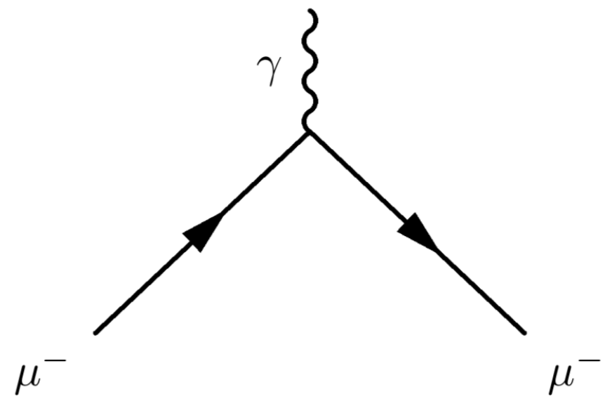
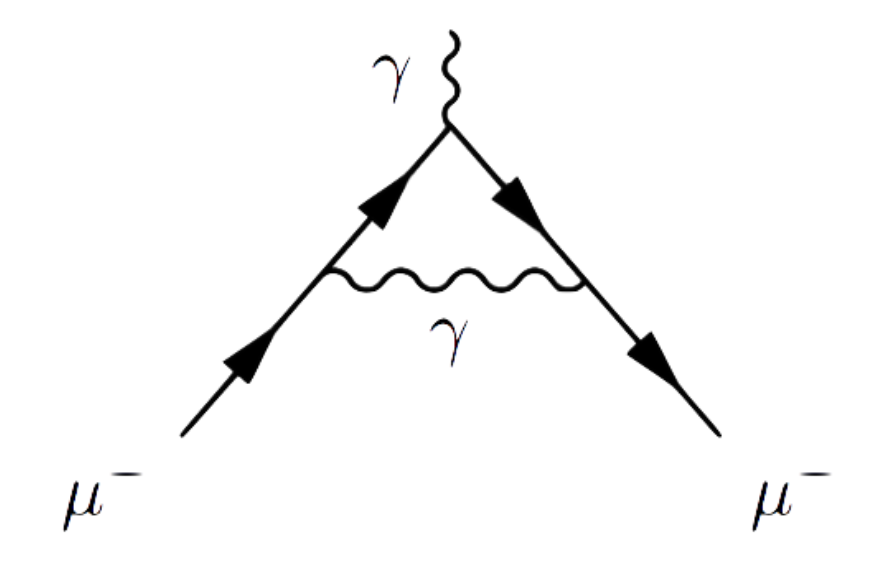

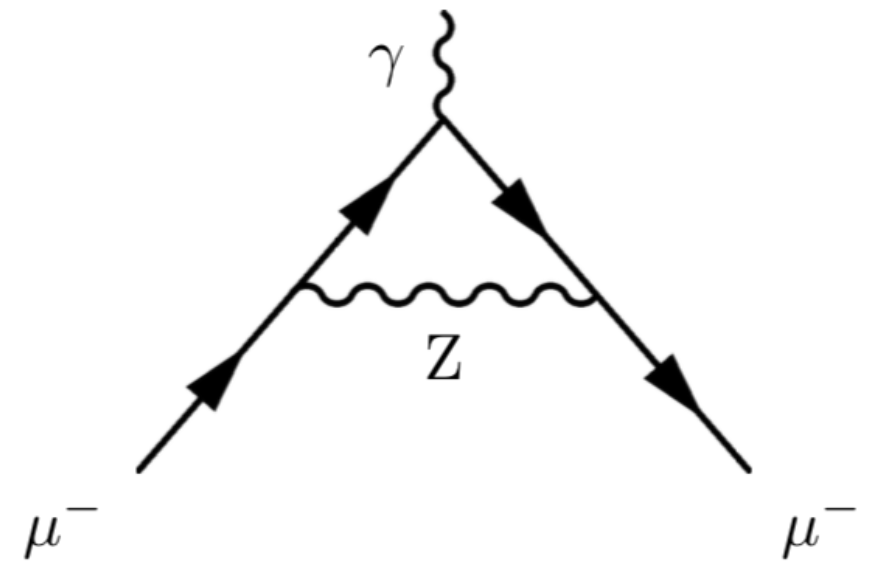
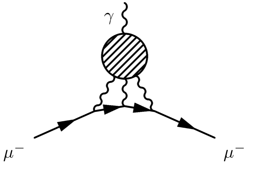
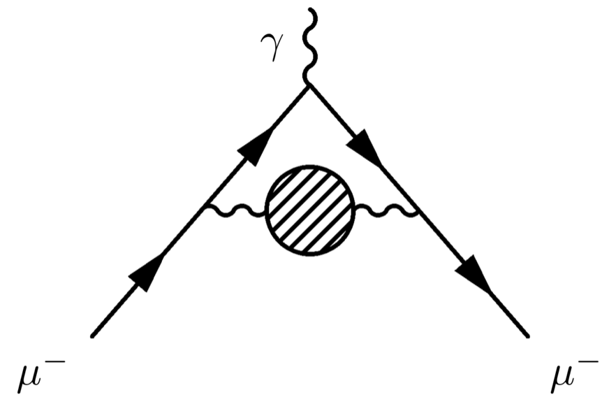
is the dominant contribution, while the uncertainty is dominated by the hadronic part (lowest order hadronic vacuum polarisation and light-by-light interactions), as shown in Figure 2.2. A more detailed account of SM contributions to , and their corresponding theoretical uncertainties, is given by T. Aoyama et al. [7] and A. Keshavarzi [8].

The theoretical accuracy of is comparable to the experimental accuracy of the previous Muon experiment at BNL, with the final result of 0.00116592091(63) [1], having a precision of 540 ppb. The difference between the BNL experiment and theory is given by
| (2.5) |
which corresponds to a deviation between the experiment and the theory of 3.7. To account for this discrepancy, a new physics correction () to may be required. One of such possible corrections, using an extension to the SM known as supersymmetry, is discussed in [9].
2.1.1 Muon’s sensitivity to new physics
Other fundamental particles, such as an electron, also posses a magnetic dipole moment, which can be used in searches for new physics. However, the contribution of the virtual particles to the magnetic anomaly, , of leptons scale with mass [10] according to
| (2.6) |
where is the mass of a lepton, and is the mass scale of new physics. Given the muon-to-electron mass ratio () of , the search for new physics with muons is much more effective than with electrons, given the relative experimental precision of these measurements.
What makes this search different, compared to the one with the electron, is the fact that the muon is an unstable particle. The muon decay channel of interest to the experiment is . This process is illustrated in Figure 2.3.
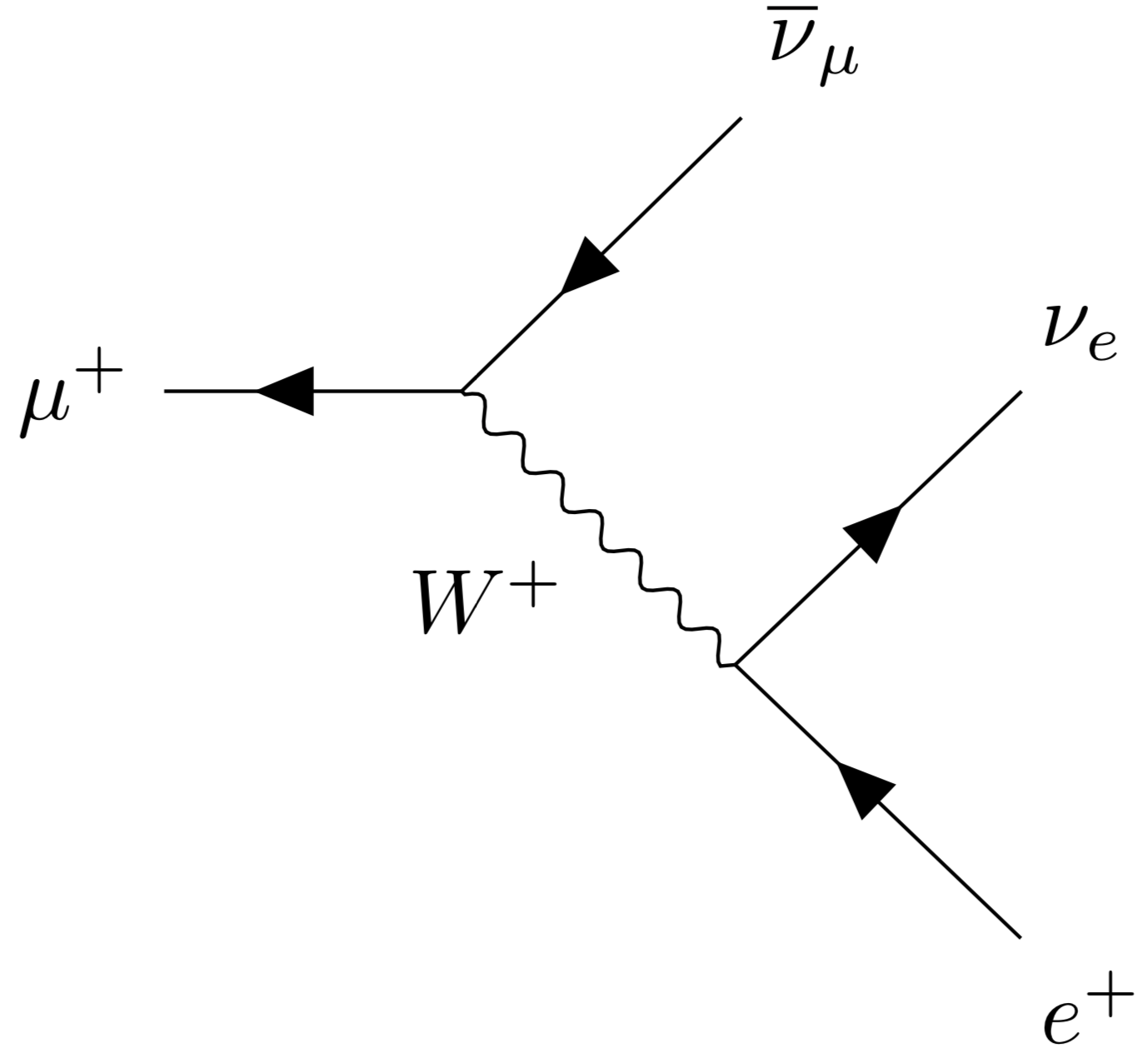
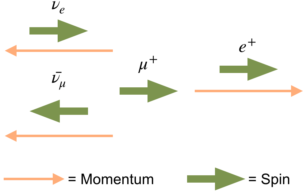
The three-body decay of the muon in Figure 2.3 provides information on the muon spin orientation at the time of the decay. The structure of the weak interaction means that the highest energy positrons from the decay of the are preferentially emitted along the direction of the muon spin.
2.2 Electric dipole moment
Analogous to in Equation 2.1, a potential muon EDM, , is defined by
| (2.7) |
where is a dimensionless constant [11], analogous to in Equation 2.1.
The SM prediction of the electron EDM, , is cm [12]. The scaling law [13] suggests that the corresponding value for the muon EDM would be
| (2.8) |
This yields a value of of cm, well below the current experimental reach. Hence, any observation of would be evidence of NP.
The goal of the Fermilab experiment is to measure with a sensitivity greater than cm [14], more than a factor of 10 improvement on the current best experimental limit from the BNL experiment [15].
The transformation properties of the dipole moments reveal an important conclusion. The Hamiltonian [6] for the muon in an applied magnetic, , and electric, , fields is given by
| (2.9) |
Transformations under time reversal (T) are odd for axial vectors (i.e. and ) and even for polar vectors (i.e. ), while the reverse is true for charge (C) and parity (P) transformations, as shown in Table 2.1.
| or | |||
|---|---|---|---|
| P | |||
| C | |||
| T |
The first term in Equation 2.9 is invariant under a T transformation
| (2.10) |
However, the second term is not
| (2.11) |
Therefore, assuming an overall CPT invariance, T violation implies CP violation. Hence, an EDM measurement by the experiment (above cm) would provide clear evidence of CP violation in the charged lepton sector. A more detailed discussion of the muon EDM is available from B. Roberts and Y. Semertzidis [6]. The methodology of the EDM measurement with the tracking detector is given in Section 10.2.
Chapter 3 The Muon experiment at Fermilab
This chapter describes the methodology of the measurement of the muon magnetic anomaly by the Fermilab experiment. Section 3.1 provides an overview of the entire experiment, with a more detailed description of the beamline, storage ring components, spatial and temporal distribution of the stored beam, magnetic field, and detectors given in Sections 3.2, 3.3, 3.4, 3.5 and 3.6. A more in-depth description of the data acquisition (DAQ) and the tracking detectors is given separately in Chapters 4 and 5, respectively, while the methodology of the EDM measurement with the tracking detector is given in Section 10.2.
The performance of the experiment in the data taking periods from 2017 to 2020 is discussed Section 3.7. The expectation for future data taking periods is also given. An overview of the experimental data reconstruction is given in Section 3.8, where data quality cuts are also discussed, along with an alternative implementation of tracker data reconstruction in the UK. Finally, the experiment’s simulation framework is described in Section 3.9.
3.1 Overview
The principal goal of the Fermilab Muon experiment is the reduction of the experimental uncertainty on the measurement of , as compared with the BNL experiment, using a measurement strategy similar to the one at the BNL [1]. This reduction in the uncertainty on will be achieved via reductions in the statistical uncertainty due to the use of the Fermilab muon beam [16], and the systematic uncertainty due to improvements in the detectors, such as the in-vacuum tracking detectors [17], and more finely segmented calorimeters [18], a better field uniformity [19], and a laser calibration system [20], as well as improved analysis techniques.
Achieving the experimental goal requires a dataset containing positrons with energies above 1.8 GeV. The momentum of the injected muons is 3.09 GeV: the so-called \saymagic momentum at which the effect of the motional magnetic field is zero (see Section 3.3.3). This momentum corresponds to a boosted lifetime of the muon of . To perform the measurement of , two measurable quantities are of interest: the anomalous precession frequency, , and the applied magnetic field, . is defined as the difference between the spin and cyclotron frequencies (see Section 3.3.3). In the case of a uniform magnetic field and negligible betatron oscillations, the relationship between , , and can be written as follows
| (3.1) |
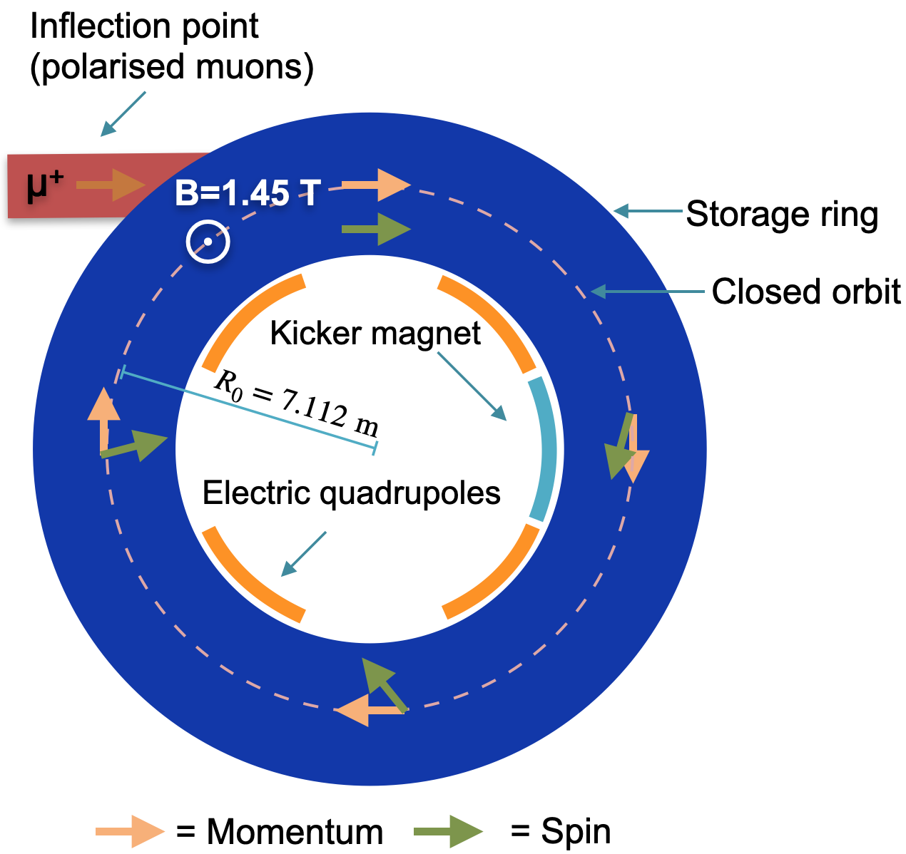
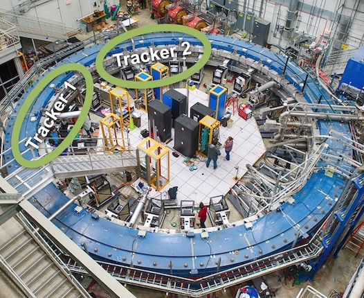
Longitudinally polarised muons are injected into the storage ring, as shown in Figure 3.1a, where they ultimately follow a circular orbit of mean radius, , of 7.112 m in the magnetic dipole field and are vertically focused using electrostatic quadrupoles (ESQs). The muon beam enters the ring through the inflector magnet, designed to cancel out the dipole magnetic field, at a slightly larger radius than the ideal orbit. The kicker magnets are used to deflect the beam onto the correct orbit.
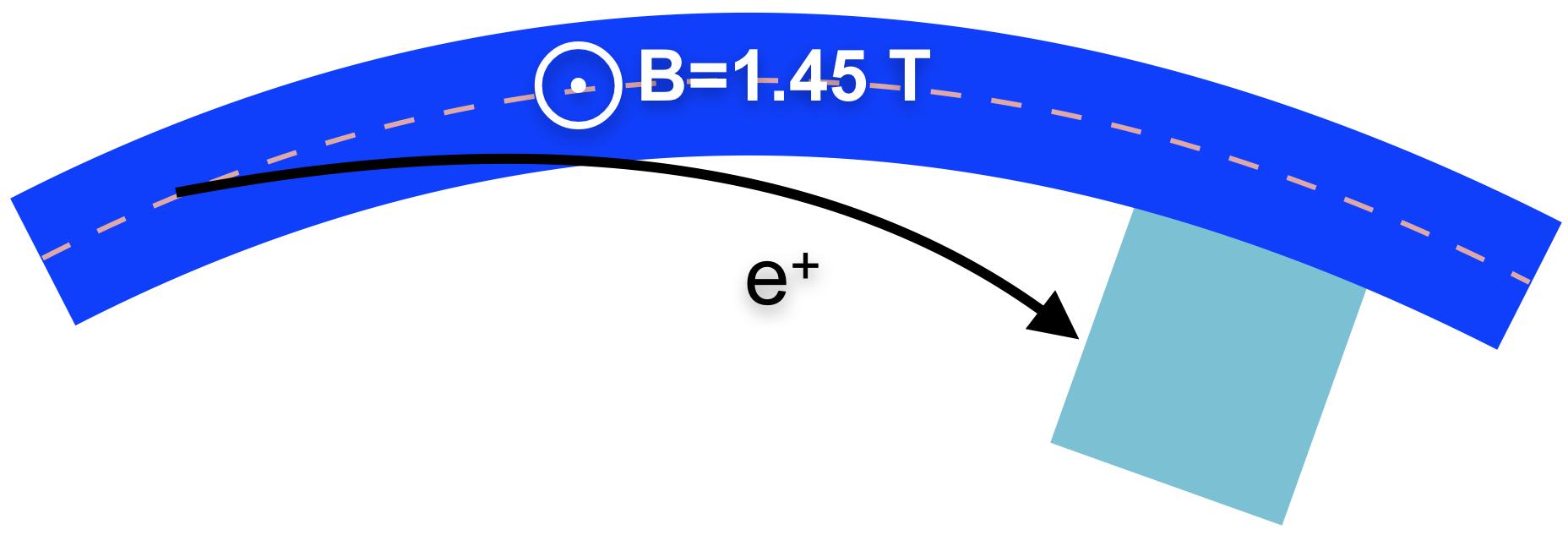
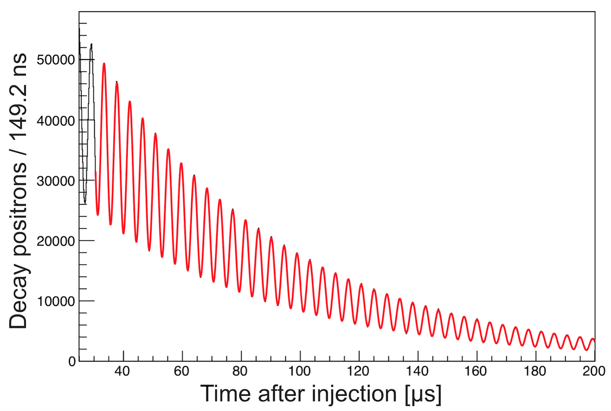
Since , the muon spin precesses faster than the momentum vector in the storage ring. Due to the structure of the weak interaction, the highest-energy positrons, from the decay of the , are preferentially emitted along the direction of the muon spin, as shown in Figure 2.3. The positrons curl inwards, where they can interact with one of the 24 calorimeters placed around the interior of the storage ring. This is shown in Figure 3.2a. High energy positron events are then histogrammed as a function of time to extract , as shown in Figure 3.2b.
The magnetic field is determined through a frequency measurement: the Larmor frequency of a free proton, . It is measured using nuclear magnetic resonance (NMR) and the relationship
| (3.2) |
where is the proton gyromagnetic moment ratio [22]. Using Equation 3.2, can be expressed as a function of the two experimentally measured frequencies and well-determined ratios
| (3.3) |
where , , and are known [22] with uncertainties of 0.00026 ppb, 3.0 ppb, and 22 ppb, respectively.
The simple harmonic motion of the stored muon beam in the horizontal plane, known as the coherent betatron oscillation (CBO) [23], contribute significantly to the systematic uncertainty on . The fraction of events where a positron is detected by the calorimeters depends on the radius of the muon beam at the point of decay. The CBO of the stored beam can thus produce an amplitude modulation in the observed positron time spectrum, as described in Section 3.4.2. One of the aims of the tracking detectors is to measure the CBO.
3.2 Beamline
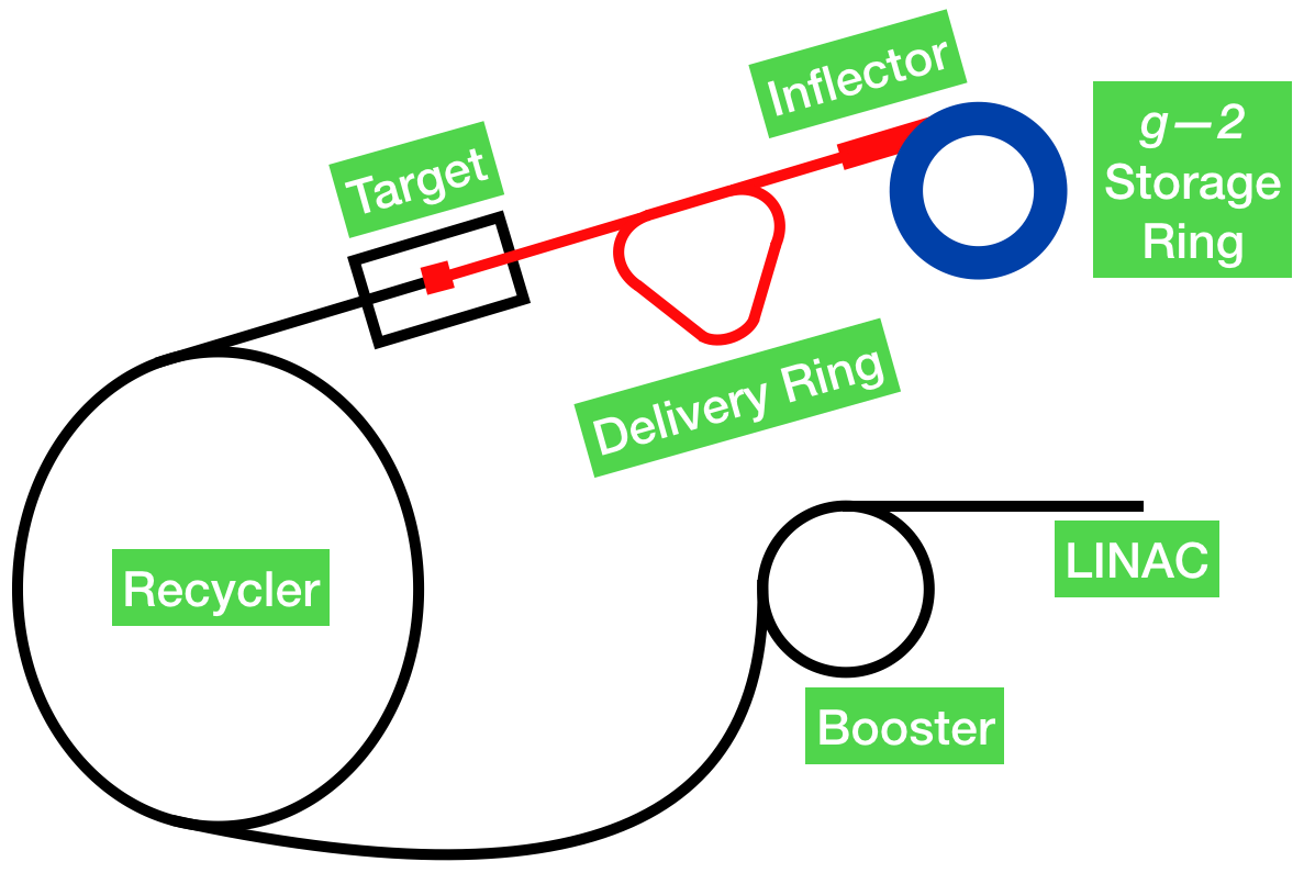
The aim of the accelerator complex, shown in Figure 3.3, is to deliver a beam of muons, which is largely free of contaminants (e.g. , , , ), into the storage ring. The muons in the experiment come from pion decays
| (3.4) |
which are produced by sending a proton beam with a momentum of 8.89 GeV– with protons in a single bunch of ns – on an Inconel 600 [24] production target
| (3.5) |
are used in the experiment, as the cross-section for production is greater than that for . Each proton bunch delivered by the accelerator complex to the pion production target corresponds to a muon fill in the storage ring. The proton beam is bunched in the Recycler to fill the storage ring optimally. The produced 3.11 GeV pions, as well as any remaining protons, undergo five revolutions in the Delivery Ring. This is done to allow all pions to decay, and to separate muons from electrons and protons, as much as possible. Further details on the beamline are given by D. Stratakis et al. [16].
3.3 Storage ring components
One muon fill () corresponds to a single accumulation of the muons and defines the measurement window for the experiment. The goal of the storage ring components described here is to keep the beam stable during this time. For a cyclotron period, , of 149 ns this corresponds to revolutions of the beam around the ring.
3.3.1 Inflector
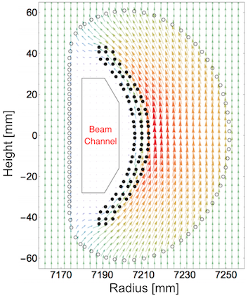
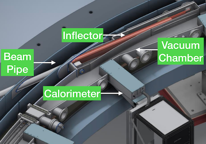
The delivered muon beam to the experiment passes through an inflector magnet which facilitates injection of the beam into the storage ring by cancelling the main magnetic dipole field (1.45 T) of the ring. The inflector provides a field-free region (beam channel) through which the injected muon beam passes without deflection, as shown in Figure 3.4. This requirement on the inflector means that the beam is injected at a angle, meaning that the actual orbit is displaced by 77 mm radially outward from the closed orbit of the storage ring. The inflector is made of niobium-titanium-copper-aluminium superalloy, with a nominal design current of 2850 A. Further details of the inflector can be found in the technical design report [11].
3.3.2 Kicker
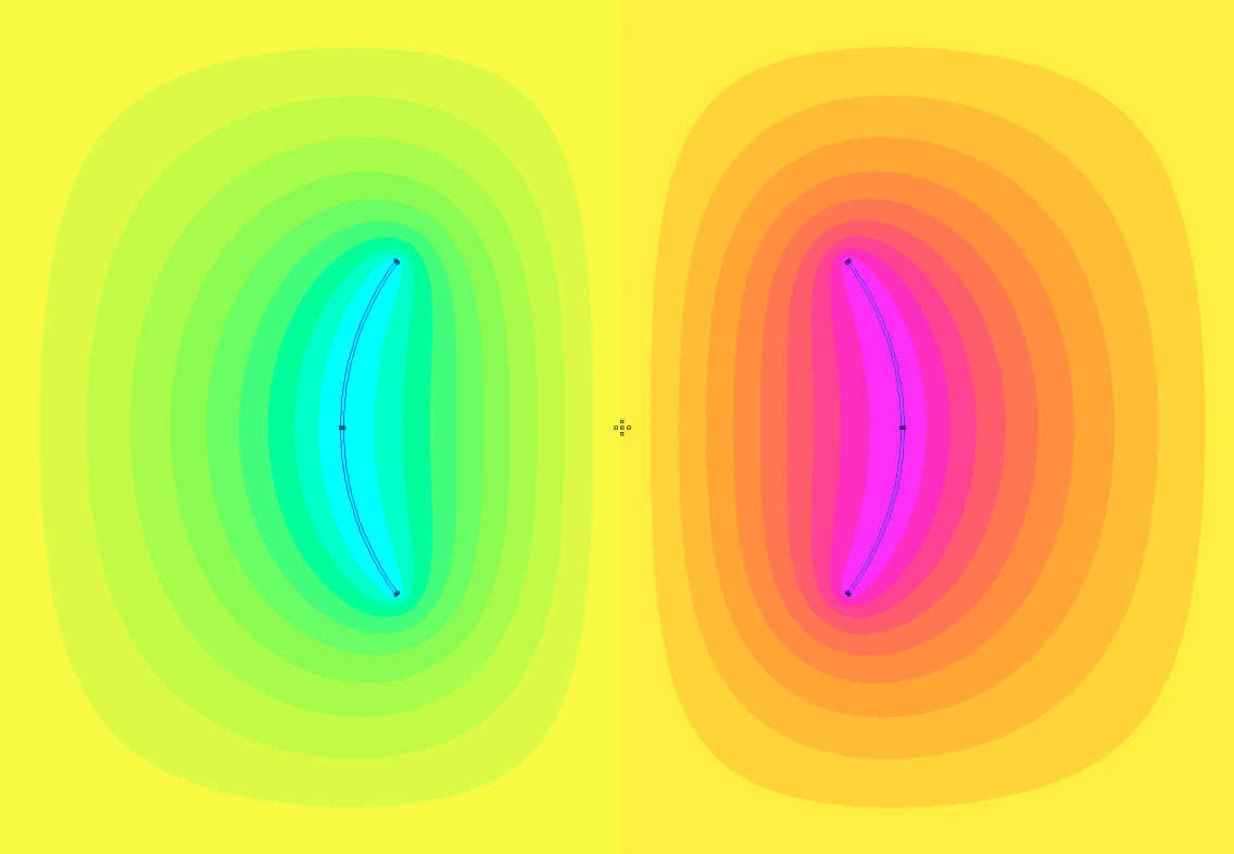
The displaced orbit instantiated by the inflector is adjusted by the fast muon kicker, as shown in Figure 3.5. The kicker is a pulsed magnet with a vertical magnetic field that directs the muons onto the ideal orbit. The kick requires an integrated vertical magnetic field of 1.2 kG-m, for ns. After which the field must return to zero before the lead muons complete a single revolution and re-enter the kicker aperture 149 ns later. The kicker is further described by A. Schreckenberger et. al [27].
The kicker and the inflector are crucial components in maximising the number of stored muons, as well as the position of the beam in the ring. Their optimisation is, therefore, critical to the operation of the experiment.
3.3.3 Electrostatic quadrupoles
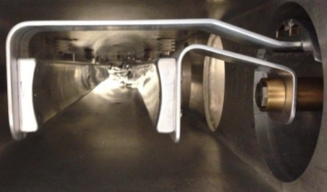
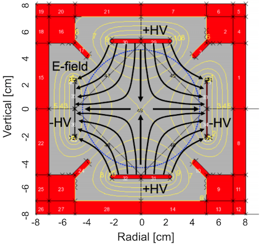
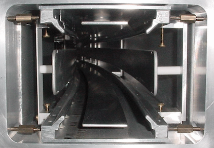
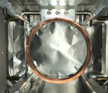
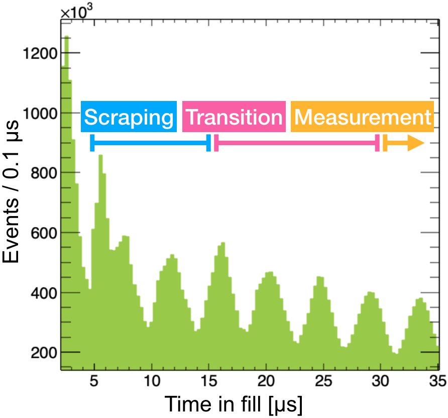
To provide a stable beam storage ESQs, as shown in Figure 3.6, are used to focus the beam vertically using an electric field of kV. Without the vertical focusing, the beam would diverge and would ultimately be lost after only a few turns around the ring. Moreover, the ESQs are used to remove stored muons that fall outside of the storage region – a process knows as scraping. This involves adjusting the voltage on the quadrupoles to scrape the beam against collimators, one of which is shown in Figure 3.7. The collimators have an inner radius of 45 mm, which defines the storage region aperture. After scraping, the beam stabilises after and can be used for measuring .
An important property of the ESQs is the so-called field-index, , which characterises the strength of the electrostatic focusing in relation to the magnetic field strength (1.45 T),
| (3.6) |
where is the electric quadrupole gradient, and is the velocity of the muon beam. In the experiment, a typical value of is , which corresponds to the so-called weak focusing mode.
The importance of the ESQs is further demonstrated by considering the measurement of . The cyclotron (149 ns) and spin precession frequencies of the muon beam are given by [6]:
| (3.7) |
and
| (3.8) |
for a muon moving in a horizontal plane of a magnetic storage ring, where is the Lorentz factor, , with the magnetic field components resolved relative to the muon trajectory. The anomalous precession frequency, (i.e. \saythe frequency), is defined as the difference of the spin precession and cyclotron frequencies, which corresponds to the rate of muon spin precession relative to the momentum vector
| (3.9) |
Assuming the muon velocities to be near perpendicular to , the inner product of . As the momentum of the injected muons has been deliberately set to the \saymagic momentum of 3.09 GeV () the last term in the Equation 3.9 vanishes. However, in reality these conditions are not realised exactly, and small corrections to Equation 3.9 must be applied. These corrections are the pitch and electric field corrections, and are discussed next. Further details on the ESQs can be found in the technical design report [11].
3.4 Spatial and temporal distribution of the stored muon beam
Several important effects arise in the storage process of the muon beam in the experiment. In this section, effects such as vertical pitch, CBO, fast rotation, closed-orbit distortions, and lost-muons are considered, as they are directly referenced in the further chapters of this thesis. The full description of the beam effects is given in [30].
3.4.1 Vertical pitch
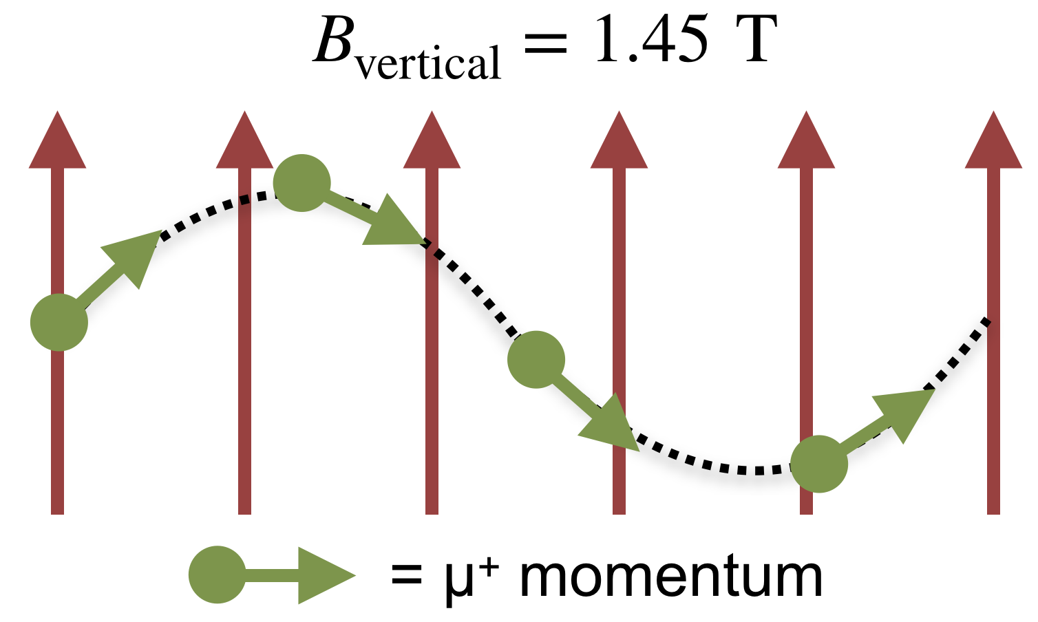
The muons in the storage ring undergo a vertical motion due to the focusing from the electrostatic quadruples, as shown in Figure 3.8a. This introduces an additional term in the expression of in Equation 3.1 that needs to be incorporated into the analysis
| (3.10) |
This changes the measured spin precession frequency, and so needs to be corrected for by the so-called pitch correction, , which is proportional to the vertical width of the beam,
| (3.11) |
is measured by the tracking detectors, as shown in Figure 3.8b.
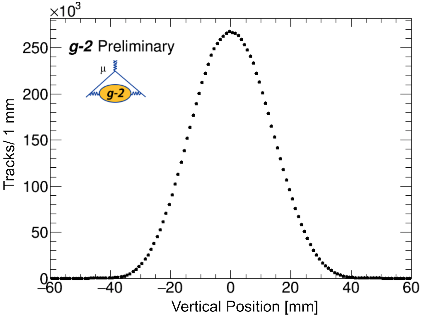
A misalignment of the tracking detectors will bias the beam measurement, and hence the pitch correction. The alignment of the tracking detectors and its impact on the pitch correction is described in Chapters 6, 7 and 8.
3.4.2 Coherent betatron oscillations (CBO)
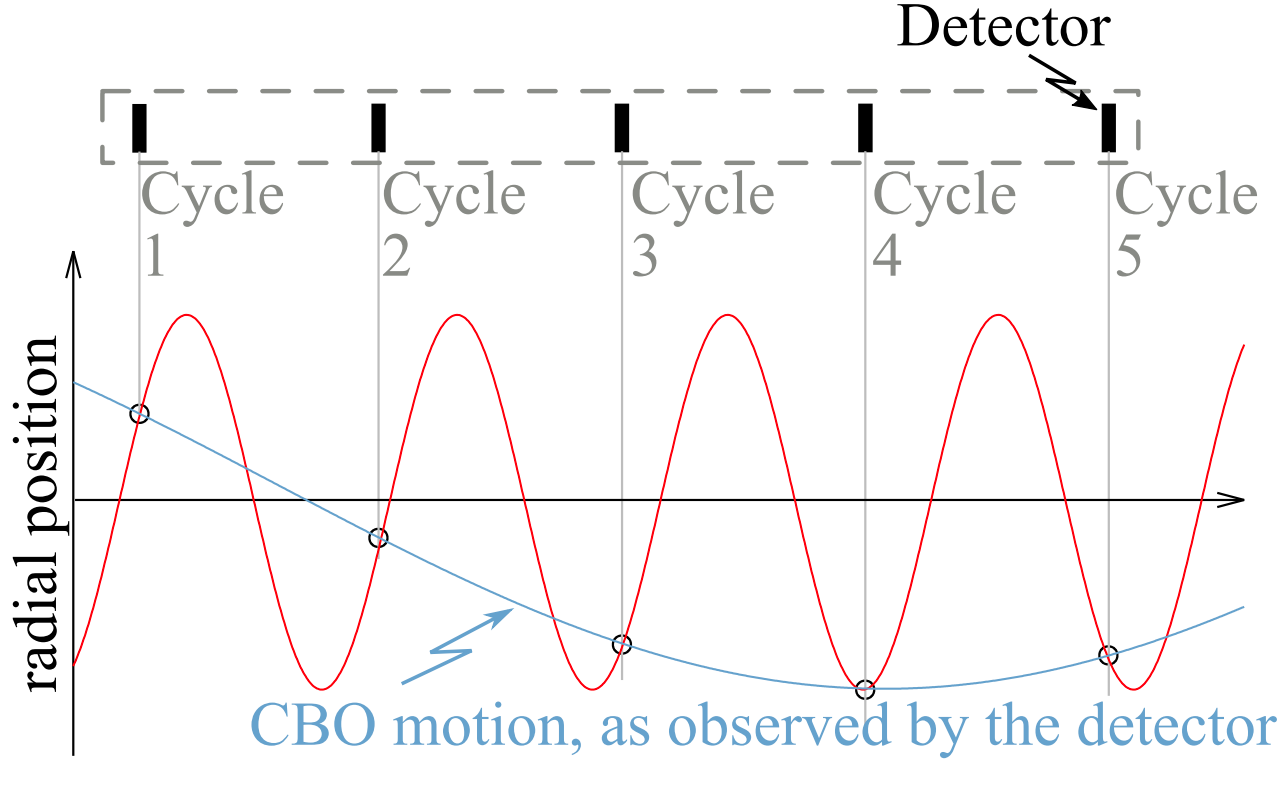
The fraction of events where a positron is detected by the calorimeters depends on the radial position of the muon beam in the storage ring. The beam has a finite momentum and position distribution, and so, any particles not having exactly the \saymagic momentum or not positioned at the ideal orbit will be subject to restoring forces from the ESQs and the magnetic field. These restoring forces cause simple harmonic motion of the beam, with the muons oscillating in-and-out radially. This results in slightly different cyclotron periods for different momenta. As each detector is effectively sampling the beam at the cyclotron frequency ( MHz),
| (3.12) |
while the radial betatron frequency ( MHz)
| (3.13) |
is larger than , there is an aliasing effect such that the radial betatron motion of the beam is instead observed as an apparent slow-moving oscillation (c.f. Nyquist frequency [32]). The actual frequency measured by a detector, as illustrated in Figure 3.9a, is
| (3.14) |
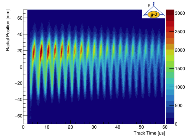
The radial position of the muon beam can be monitored as a function of time using the tracking detectors, as shown in Figure 3.9b, in order to estimate the amplitude and frequency of the CBO.
Analogous to the CBO is the so-called vertical waist (VW), with the corresponding vertical betatron frequency ( MHz)
| (3.15) |
Since is smaller than , the VW oscillation
| (3.16) |
is measured directly by the detectors (i.e. there is no aliasing effect), as described in more detail by T. Halewood-Leagas [34].
Both the CBO and VW oscillations must be accounted for in the analysis: if these effects are not included, then significant residuals between the data and the fit to data, as discussed in Chapter 10, are obtained.
3.4.3 Fast rotation and electric field corrections
To account for the fact that not all stored muons have the \saymagic momentum, an electric field correction [11], , to Equation 3.9 is implemented
| (3.17) |
where
| (3.18) |
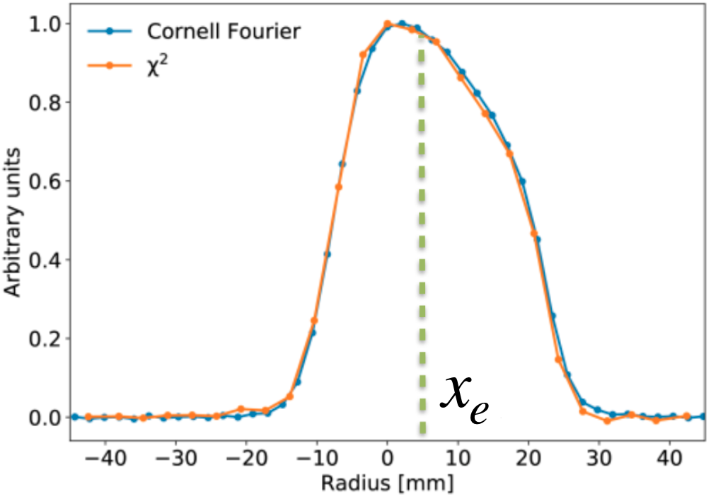
and is the equilibrium radius of the beam (i.e. the average radial position of the beam), and is the radial width of the beam. and are extracted directly from the so-called fast rotation analysis, as shown in Figure 3.10a, which considers how stored muons at various momenta cause \sayde-bunching of the beam. For example, for a group of muons with momentum larger than the \saymagic momentum, the stored orbit will have a larger radius leading to a larger . The methodology of the fast rotation analysis is described in [35].
3.4.4 The effect of the CBO and on the beam
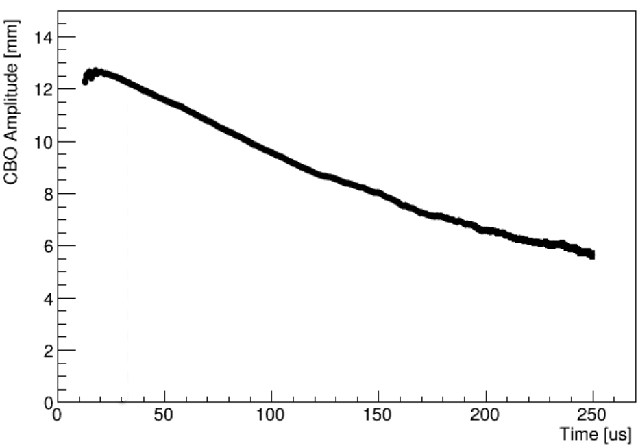
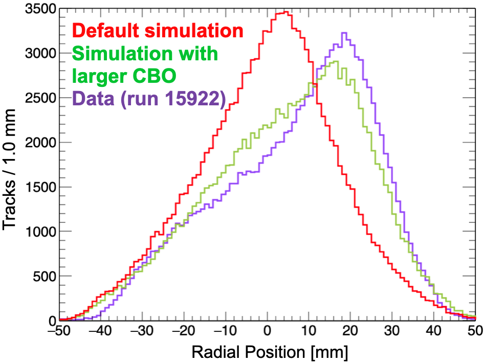
The mean stored radial beam position is slightly larger than expected, due to the kicker providing a field below the design value. This is implemented in the simulation using data-derived parameters for , using the fast rotation analysis, and the radial CBO amplitude, as measured by the tracking detectors, as shown in Figure 3.10b. Using the measured CBO and produces a more realistic radial beam profile in the simulation, as shown in Figure 3.11, where it is compared with the default simulation and data.
3.4.5 Closed-orbit distortion
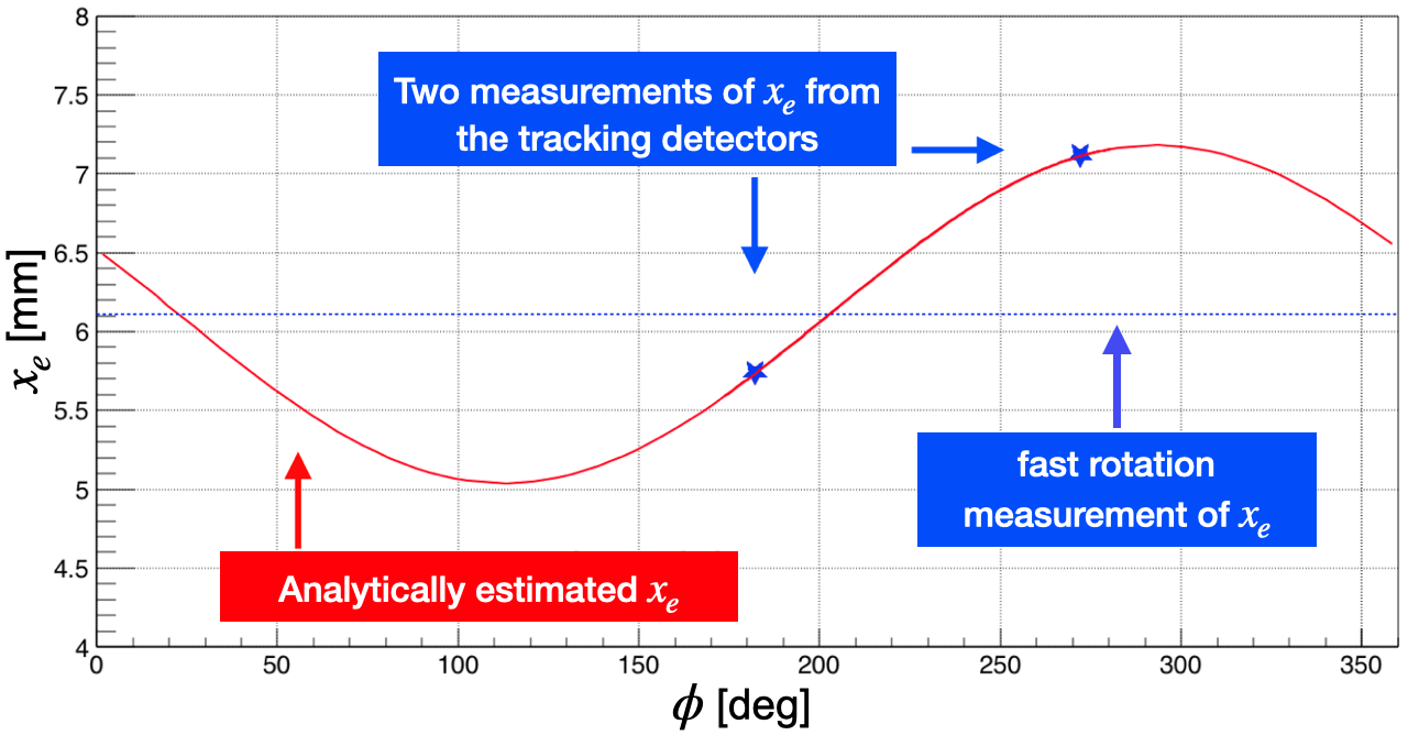
Another assumption in Equation 3.9 is the uniformity of the magnetic field throughout the ring. In practice, the field has small inhomogeneities, which contribute to an effect known as closed-orbit distortion, which results in different equilibrium positions of the beam around the ring. That is, varies with azimuth. The analytically estimated [36] model and three measurements of are shown in Figure 3.12. Two of these measurements come from the tracking detectors: each detector observes different segments of the beam’s orbit. These measurements are sensitive to the global alignment, as described in Appendix A. Further details on the closed-orbit effect are presented in [36].
3.4.6 Lost-muons
Some of the stored muons in the ring will interact with material (e.g. collimators) emitting radiation and losing energy. These so-called \saylost-muons will curl inwards towards the centre of the ring and exit the storage ring. However, some of them will still deposit a small amount of energy in the calorimeters and fail the energy cut. Matching calorimeter and tracker measurements via can be used to distinguish between and , as discussed in Section 5.3. A corresponding systematic uncertainty on the measurement of arises from time-dependence and momentum-dependence of the muon loss. Both of these effects introduce a time-dependent phase that biases . Further details on the study of lost-muons are given in [37].
3.5 Magnetic field system
The magnetic field system aims to produce a uniform vertical magnetic field of 1.45 T and to measure it with an uncertainty of ppb. This measurement is performed in the cross-section of the storage region, as shown in Figure 3.13a, in the volume of 1.1 m3.
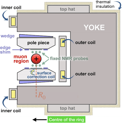
A formidable technical challenge was the so-called \sayshimming of the superconducting magnet, which involved physical modifications of the magnet to set a uniform field around the ring. The result of this procedure is shown in Figure 3.14.

To further refine the uniformity of the magnetic field, as well as to ensure stability over time, an active shimming was implemented. This was done using a power supply feedback to keep the dipole field constant using correction coils to smooth the field. This process achieved the field uniformity of 1 parts-per-million (ppm) [29], with the correction coils shown in Figure 3.13b.
When the muons are not stored in the ring, the magnetic field is measured by a trolley system, which contains 17 NMR probes. The trolley completes a full revolution around the ring in approximately three hours every three days to map the field profile in the storage region, as shown in Figure 3.15 for one azimuthal location.

When the muons are injected, the field is continuously measured by fixed NMR probes located outside of the storage region. This is done in order to track the field between the trolley runs. This field map is then convoluted with the beam profile (see Section 5.3.7) measured by the tracking detectors to find the average field experienced by the muons before decay.
Further details of the field measurements, including the absolute field calibration, and the relative trolley calibration using a plunging probe, are given in [40].
3.6 Detectors
An in-depth description of the DAQ and the tracking detectors is given in Chapters 4 and 5, respectively, while the calorimeters and the auxiliary detectors are described in more detail in [41], as well as in the technical design report [11].
3.6.1 Calorimeters
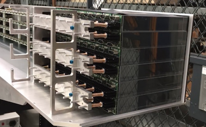
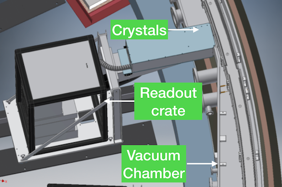
The measurement will be realised by 24 electromagnetic calorimeter detectors, which are distributed uniformly on the inside of the storage ring. Each calorimeter comprises 54 segmented lead-fluoride Cherenkov detectors, as shown in Figure 3.16. Each crystal is read out by a Hamamatsu silicon photomultiplier (SiPM), which are constantly gain-calibrated between the muon measurements by a laser calibration system [20]. The calorimeters measure the energy and time of arrival of the positrons, from the muon decay.
The largest single systematic uncertainty associated with the calorimeters is pileup, which occurs when, for example, two low energy positrons deposit energy in the same crystal close together in time (within ns). The tracking detectors can be used to investigate pileup in the adjacent calorimeters, as they can reconstruct independent trajectories of the positrons. The final goal for a systematic uncertainty on the measurement is 70 ppb, while the experimental goal of collecting positrons corresponds to a statistical uncertainty of 100 ppb. Combining the statistical and the systematic uncertainty from the determination of in quadrature with the field measurement uncertainty gives the total experimental design uncertainty of 140 ppb.
3.7 Data-taking periods
3.7.1 Commissioning run
To ensure that all components of the experiment were performing adequately, a commissioning run, which lasted from 31 May 2017 until 7 July 2017, was undertaken to collect preliminary data. During the commissioning run, protons and pions were also delivered to the storage ring, in addition to muons. This was due to the Delivery Ring not being used.
3.7.2 Run-1, Run-2 and Run-3
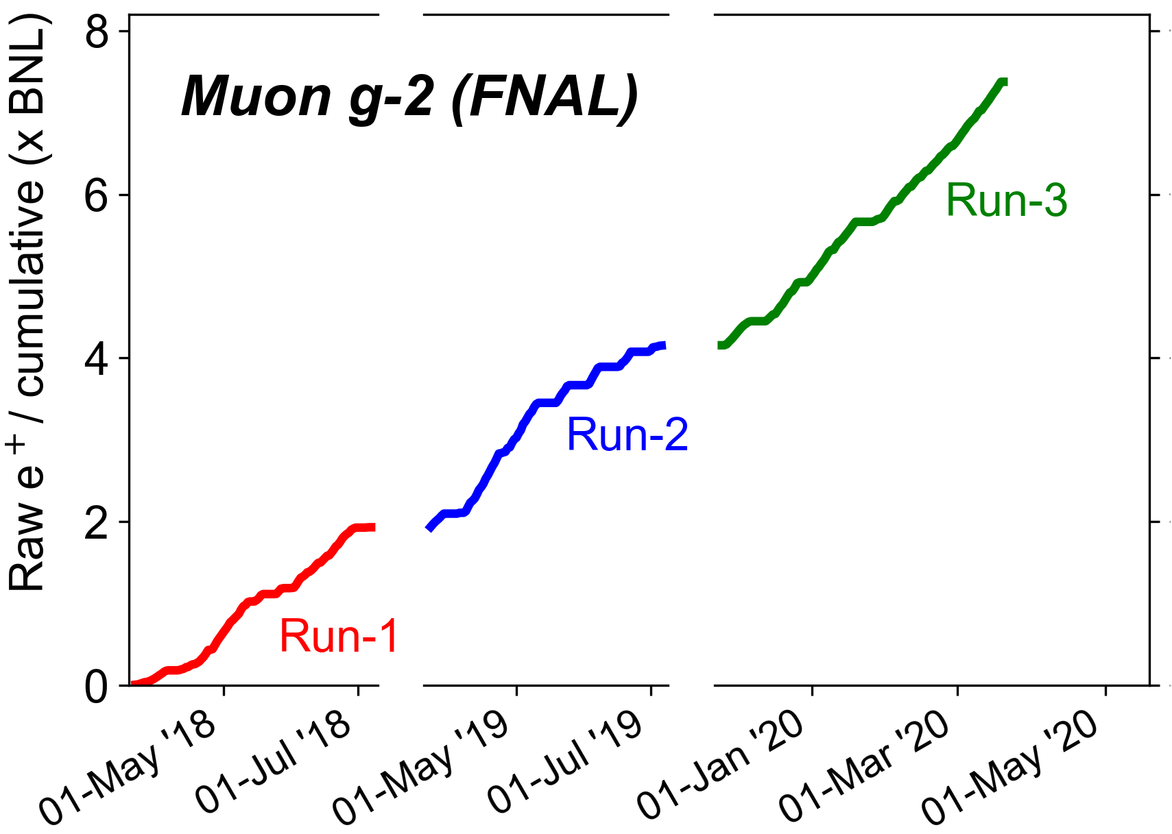
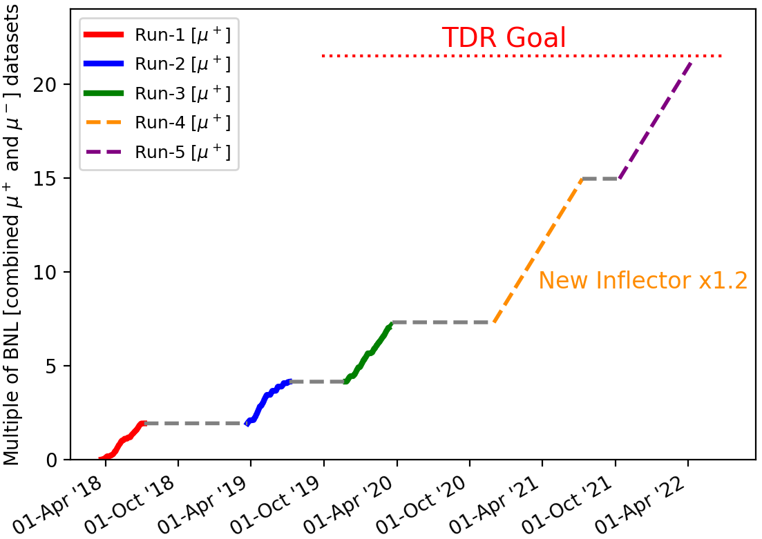
The first data-collection period (i.e. Run-1) happened from 25 March 2018 until 8 July 2018, Run-2 took place from 23 March 2019 until 5 July 2019, while Run-3 happened between 25 November 2019 and 19 March 2020. The total number of collected in these periods, as a fraction of the total number collected at the BNL, is shown in Figure 3.17a.
The work in this thesis will primarily focus on analysing the Run-1 data, as described in Chapter 10. Run-1 and Run-2 data has also been used to check the calibration of the tracking detectors as described in Chapter 7.
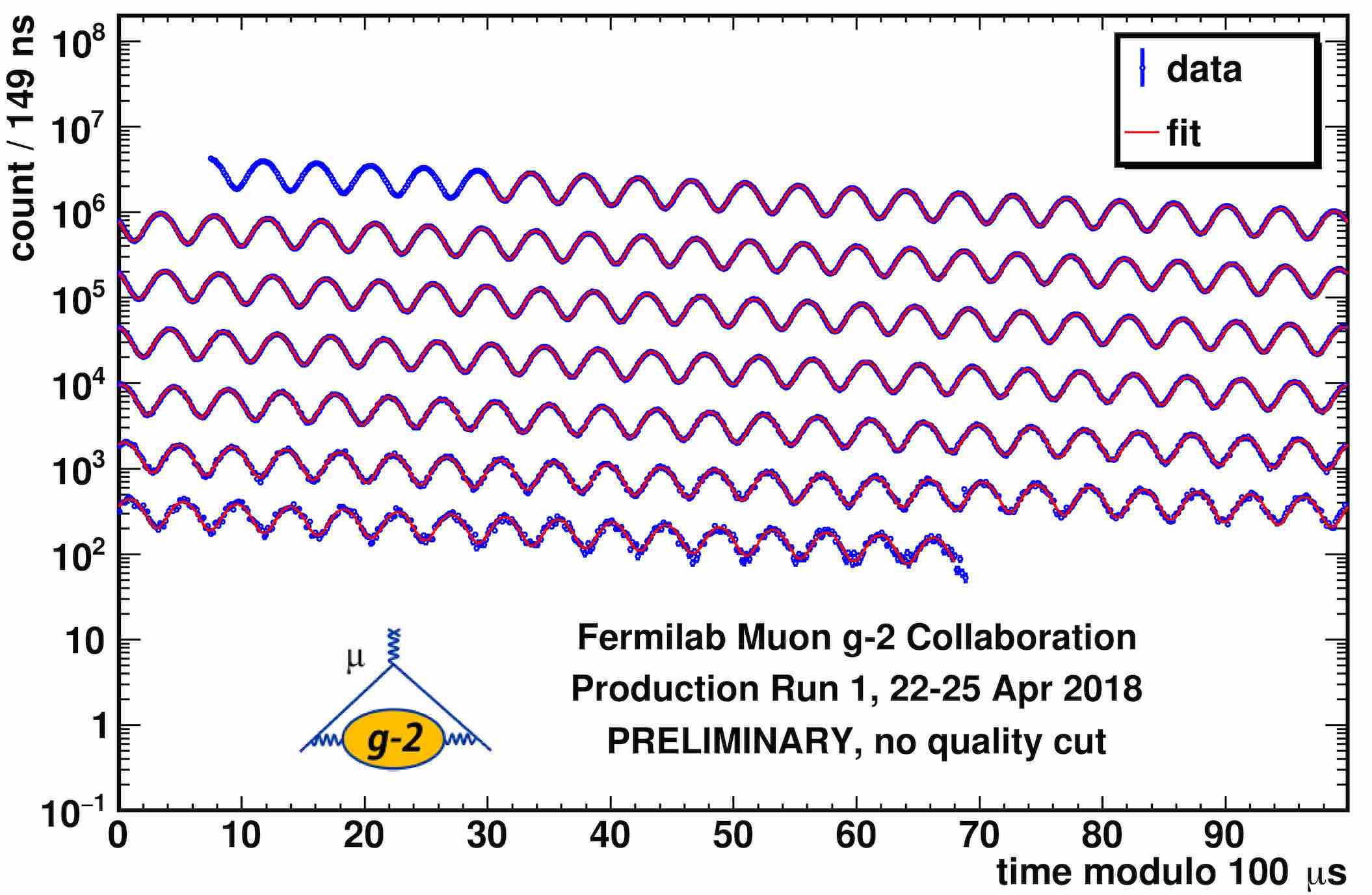
The datasets collected in Run-1 are summarised in Table 3.1, with a preliminary analysis-level plot of the 1a dataset shown in Figure 3.17b. The total amount of raw data collected, that will be used for the analysis, is roughly 0.5 PB in Run-1.
| Dataset | Number of | Raw data | field | |
|---|---|---|---|---|
| name | ( GeV) | tracks | size [TB] | index, |
| 1a | 55 | 0.108 | ||
| 1b | 75 | 0.120 | ||
| 1c | 113 | 0.120 | ||
| 1d | 273 | 0.108 | ||
| Total | 516 | - |
3.7.3 Run-4 and beyond
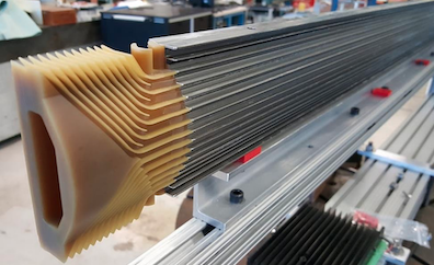
The next run will begin in December 2020 and will accumulate positrons at a higher rate due to the use of a new upgraded inflector [26], which is shown in Figure 3.18. The new inflector will increase the number of stored muons by per fill.
3.8 Data reconstruction
Given the large amount of raw data collected by the experiment, an automated process, known as \saydata production[44], which involves data transfer, reconstruction and calibration, is used, as demonstrated in Figure 3.19. Technologies such as dCache and sequential access via metadata (SAM) [45] allow for robust storage and cataloguing of data.
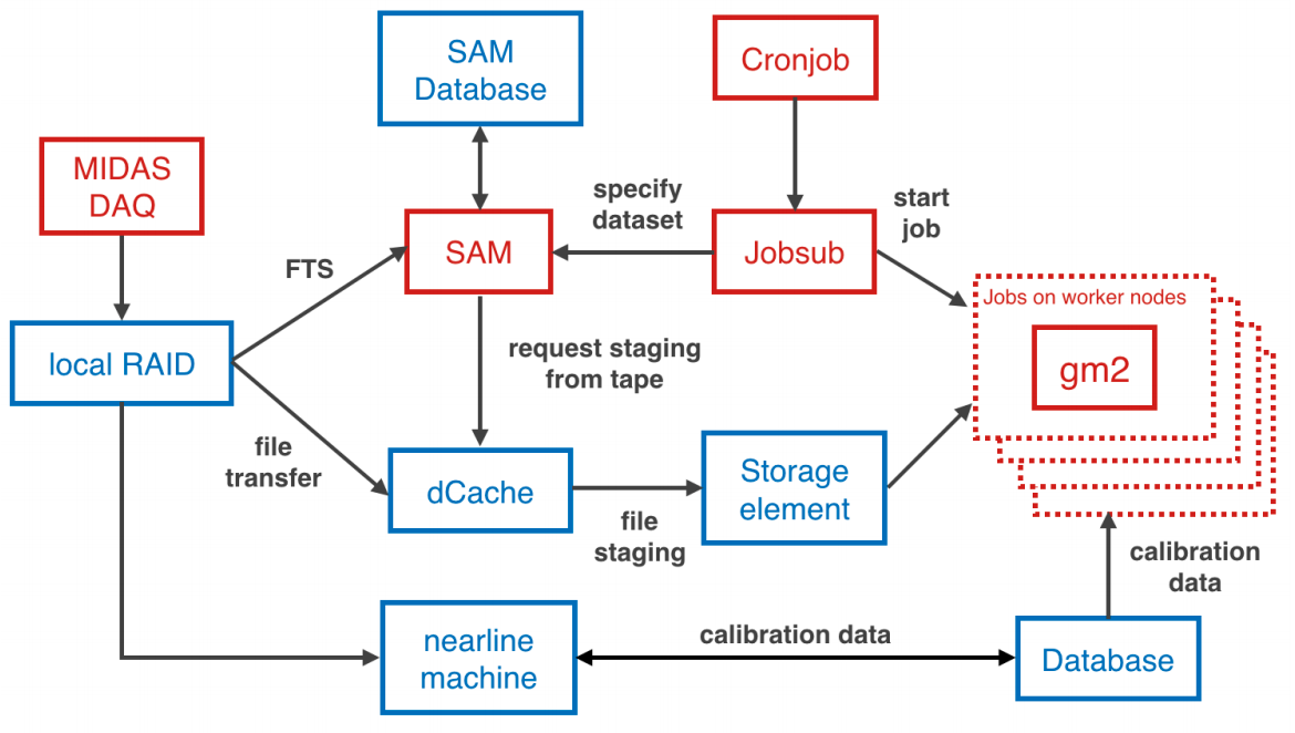
The CPU-intensive process of data reconstruction involves the processing of raw data to form physics-level data objects (e.g. tracks). This process is facilitated using distributed computing resources on the FermiGrid [46] and the Open Science Grid (OSG) [47]. To simplify this workflow, a Production Operations Management Service (POMS) [45] is used, that allows automated scheduling and monitoring of data production.
3.8.1 Data quality control
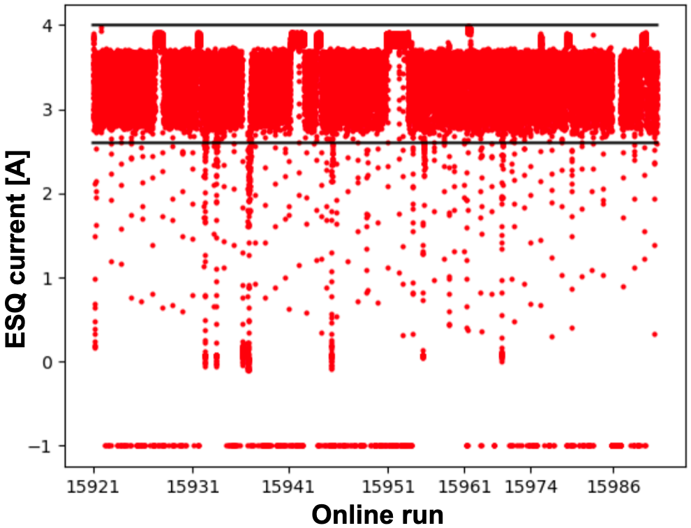
It is essential that all data used in the analysis (c.f. Table 3.1) is of good quality. This good quality condition is defined by all subsystems of the experiment performing at their nominal operational settings. If an apparatus, for example, the ESQs, recorded an abnormal drop in its current, the recorded data during this time is marked as being of bad quality and is not used during the analysis. This is shown in Figure 3.20.
3.8.2 Track reconstruction in the UK
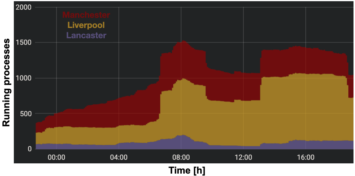
The processing of large datasets is an intensive and costly task. In the context of the data reconstruction, the tracking algorithms use up to of the CPU, while only accounting for of the raw data volume. Therefore, the addition of extra grid computing resources dedicated to tracking is well-motivated.
In Run-2, 3 TB of raw track data was recorded, while the reconstruction step will produce 50 TB of track data. To facilitate this, grid nodes at the UK universities in Manchester, Liverpool and Lancaster were added to the \say pool, as shown in Figure 3.21. Singularity [49] was used to ensure that the software could execute on the UK grid nodes.
3.9 The simulation framework
A simulation framework is essential in understanding the performance of the experiment. This framework is a C++ code-base, that relies on Fermilab’s central software infrastructure, art [50], which distributes external software products (e.g. ROOT [51] and Geant4 [52]). The geometry of the detectors, in Geant4, is used both during particle generation and during data reconstruction, for both simulated and non-simulated data. The geometry of the storage ring in Geant4 is shown in Figure 3.22.

Chapter 4 Data acquisition system
This chapter describes the DAQ system of the experiment in Section 4.1, while a detailed description of the tracking detector readout electronics is given in Section 4.2.
4.1 DAQ overview
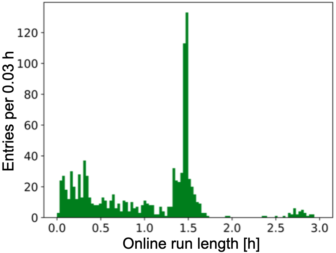
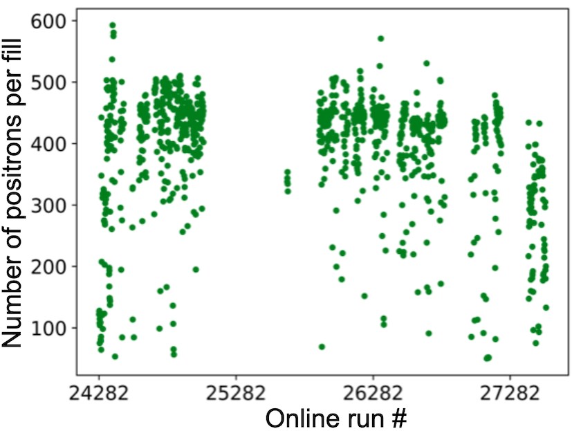
An essential component of the experiment is the DAQ system [54], which manages the data flow from the detector electronics. In addition, the DAQ interfaces to the accelerator signals (triggers) and distributes a clock. The experiment is acquiring raw data at a rate of 20 GB/s. This is accomplished by employing a parallel data-processing architecture using 28 high-speed GPUs (NVIDIA Tesla K40) to process data from 12-bit waveform digitisers, reducing the recorded (to tape) data rate to 200 MB/s. The system processes data from 1296 calorimeter channels (54 channels per calorimeter), two straw tracker stations, auxiliary detectors, the kicker, ESQs and NMR probes. The total data output of the experiment to tape during Run-1 was 2 PB. Additionally, a PCI-based GPS synchronisation card is used to timestamp the digitised data to facilitate subsequent matching between the detector system readout and the magnetic field readout. The DAQ system achieved uptime in Run-1, with nearly twice the amount of collected data compared to the E821 experiment, as shown in Figure 3.17a. The DAQ performance in Run-2, in terms of the online run length and the number of recorded per fill, is shown in Figure 4.1.
Each proton bunch delivered by the accelerator complex (see Section 3.2) to the pion production target corresponds to a muon fill in the storage ring. One muon fill corresponds to a single accumulation (i.e. triggered time window). DDR3 memory blocks allow the data from multiple triggers to be buffered in hardware, which allows the exploitation of the periodic long gaps between muon fills for asynchronous readout. The readout is decoupled from the trigger sequence (in time) to avoid buffer overfill, thus preventing back-pressure on the upstream components. The fill structure is shown in Figure 4.2.

During the data-taking periods, two shifters are always present in the control room of the experiment. The shifters control and monitor the data flow from the detector systems. This control is implemented via a state machine interface implemented in MIDAS [55]. In addition to shifters, 24/7 on-call experts for the DAQ, as well as the other subsystems, are available to ensure any software or hardware issues are solved in a timely fashion.
4.1.1 Data quality monitoring
To ensure that there are no issues during the data-taking, it is desirable to reconstruct and analyse a fraction of newly-recorded data. A data quality monitoring system [41] assesses the performance of the experimental subsystems in real-time, as shown in Figure 4.3.


4.1.2 Clock blinding
A common practice in scientific investigations is to try and reduce cognitive bias by \sayblinding the data. In the experiment, this is achieved in hardware by offsetting the MHz master clock, shown in Figure 4.4.
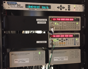
The clock is offset by a frequency , which shifts the measured value of (and ) by as much as ppm. This process is known as absolute blinding. is monitored to prevent any drifts in the blinding signal, as described in [57]. The absolute blinding is augmented by an additional software blinding, shifting in the uniform range of ppm with an additional ppm Gaussian tail. The net shift in the value of due to this double-blinding is by design larger than the previous measurement’s discrepancy with the theory of ppm (see Section 2.1).
In fitting the periodic variation of the number of decay positrons in the so-called \saywiggle plot (e.g. Figure 3.17b) to determine , a parameter is defined
| (4.1) |
where , and is expressed in ppm. The value of returned in fitting has the additional software blinding, , which is different for each analysis team, such that
| (4.2) |
Different analyses can be compared by setting , whilst still retaining the hardware blinding.
4.2 Tracking detector DAQ
This section describes the readout electronics of the tracking detector, as well as the testing and commissioning of the tracking detector DAQ at Fermilab. A more in-depth description of the development, testing and characterisation of the DAQ for the tracking detector is given by T. Stuttard [17].
4.2.1 Readout electronics
4.2.1.1 Front-end electronics
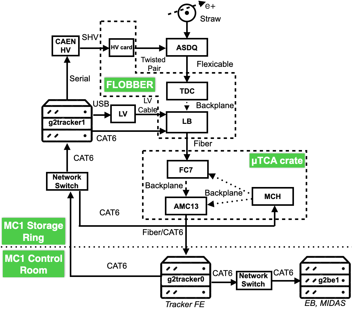
The schematic of the front-end (FE) electronics is given in Figure 4.5.
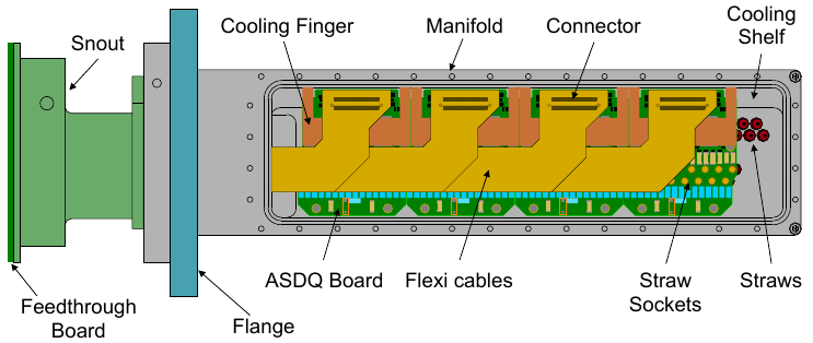

The amplified shaper discriminator charge (ASDQ) [58] cards are located inside the top and bottom manifolds. The ASDQ processes an analogue signal from a straw, and sends a digital signal to the time-to-digital converter (TDC) board via a Flexicable. Moreover, the ASDQ filters the high voltage (HV) from the HV boards to the straws. A logic board serves as an interface between the TDC and the back-end (BE) electronics. The electronic boards external to the gas volume (i.e. the manifold) reside in the front-end low voltage optical box to back-end readout (FLOBBER).
4.2.1.2 Back-end electronics
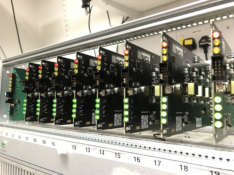
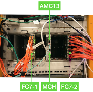
A fibre cable, connected to a logic board, passes digitised data from all the tracking detectors in a station to the FC7 [59] card in the TCA [60] crate (Vadatech VT891). An AMC13 [61] card receives the data from the two FC7 cards (one per station), via a backplane, and transmits data to a local PC, which in turn passes it to the Event Builder on a single BE machine, on which a central run-control framework – MIDAS – is run. The AMC13 is also connected to the 40 MHz external master clock. A second tracker PC provides control of the HV, low voltage (LV) and slow control (SC) via USB serial interfaces. The MCH [60] in the TCA crate monitors and controls the FC7, AMC13, and manages the crate cooling. This readout chain is depicted in Figure 4.6.
4.2.2 DAQ development at UCL
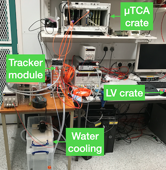
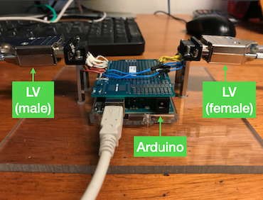
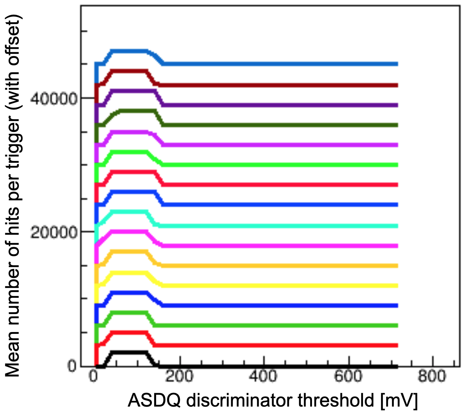
The FE electronics require a steady input of V. The LV system was developed by engineers at UCL, and was integrated into the tracker test-station, as shown in Figure 4.7. Connections between the LV system and logic boards are made via cables with D-sub (9-pin) connectors, which were installed at UCL. To ensure the integrity of cables and connectors, an Arduino LV test-stand was developed, as shown in Figure 4.8a. The tracker test-station was used to integrate and test DAQ components. One of the most common tests performed is an ASDQ threshold scan shown in Figure 4.8b.
4.2.3 DAQ commissioning at Fermilab
The BE electronics was assembled and tested at Fermilab as shown in Figure 4.9. The commissioning of the FE electronics and tracking detector itself is described in Section 5.2. The first data from the stored muon beam was acquired on 2 June 2017.

Chapter 5 Tracking detector
This chapter describes the hardware and software infrastructures of the tracking detector. The methodology of the EDM measurement using data from the tracking detector is given in Section 10.2.
5.1 Overview
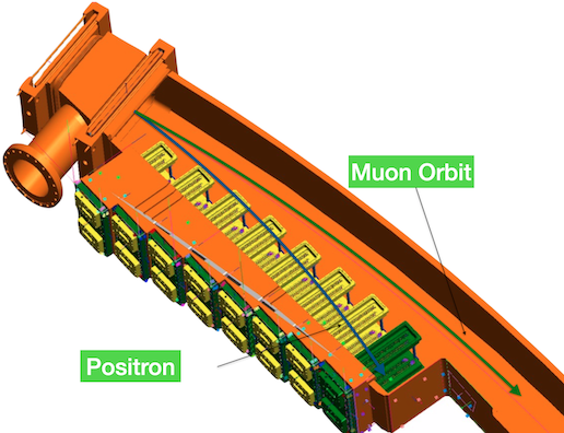
The primary aim of the tracking detector is to reduce the systematic uncertainty on via a measurement of the muon beam profile and its evolution with time. The geometry and the material of the straws are designed to minimise the energy loss and scatter of positrons. The tracking detector, shown in Figure 5.1, measures the trajectory of the positron from the decay in the storage ring. Each tracker module consists of four layers of 32 straws oriented at to the vertical. Each aluminised mylar straw is thick, and is held at 1 atm pressure. Each straw is filled with a 50:50 Ar:Ethane mixture and contains a central wire that is held at a kV potential. The modules are inside the vacuum of atm and experience a predominantly vertical magnetic field. The magnetic field in the tracker region varies radially from T – at the closest point to the stored muon beam – to T. Eight tracker modules make up a tracker station, as shown in Figures 5.2 and 5.3, with the two stations, labelled S12 and S18, located in front of two calorimeters, as indicated in Figure 3.1b.


5.2 Hardware
The design, manufacture and testing of the tracker modules were done by a team of engineers and scientists at the University of Liverpool, with a detailed description of the process available in [34, 62, 63].
5.2.1 Commissioning at Fermilab
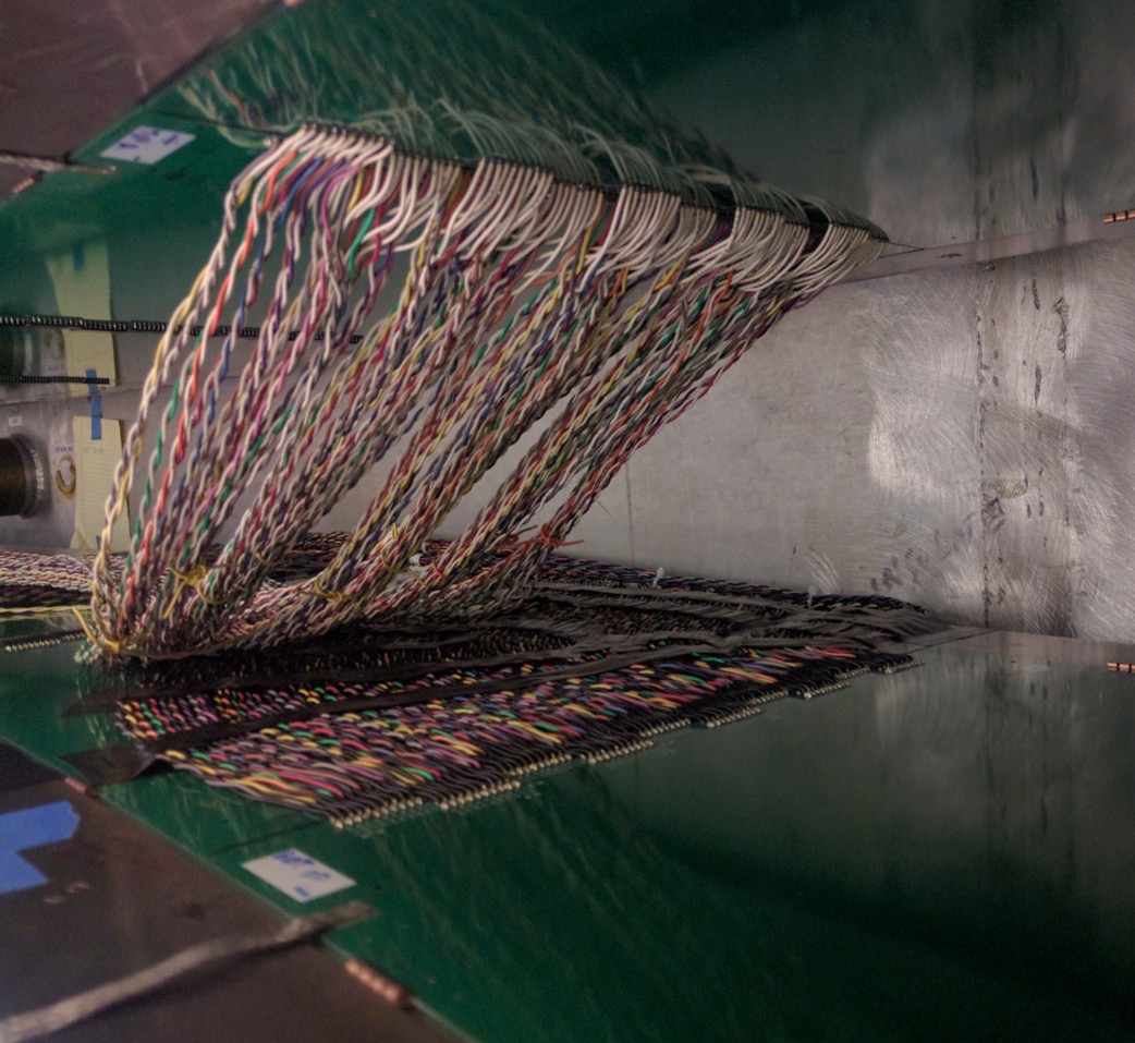
The assembly and commissioning of the detector components took place at Fermilab, with the assembled detector system ready for the June 2017 commissioning run. The installation of FE electronics into the FLOBBER units are shown in Figure 5.4.


Figure 5.5 shows the FE electronics outside of the vacuum chamber, while Figure 5.6 provides a view of the active tracking region inside of the vacuum chamber.


5.3 Software
The actual measurement that is being made by the tracker is the time a charged particle traversed a straw – the hit time. This time needs to be correlated with the mean hit time across multiple straws to calculate the so-called drift-time in a straw. The drift-time is then used to calculate the distance from the central anode wire that the charged particle passed in a given straw. A combination of multiple hit distances allows a reconstruction of the trajectory of that particle. The reconstructed trajectory allows for the measurement of the particle’s momentum, as well as – via \saytrack extrapolation – an estimation of where the decay producing the took place.
5.3.1 Hit formation
The detected signal in the tracker comes from the collected charge on the central wire in the straw. This charge is due to the ionisation electrons, liberated from Ar atoms by a charged particle traversing the straw. The liberated electrons drift towards the wire, which is held at kV. The net drifting motion of the liberated electrons is curved due to the presence of the magnetic field. The produced charge signal on the wire will be digitised and the drift-time recorded, if the pulse passes the threshold set by the discriminator. The absolute hit position in the straw is not known, only a drift circle is determined, a radius of which is given by the distance of closest approach (DCA), as illustrated in Figure 5.7 in a 2D representation through a cross-section of a straw.

The radius of the drift circle is inferred from the time-to-distance relationship shown in Figure 5.8a. The shape of the drift-time distribution is shown in Figure 5.8b, where three efficiency regimes are apparent: there are fewer hits with small and large drift-times, corresponding to the hits close and far away from the wire, respectively. The closer tracks produce fewer secondary ionisations, while tracks close to the straw wall produce fewer primary ionisations.


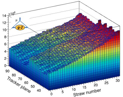
The hit occupancy distribution in both stations is shown in Figure 5.9, where no cuts are applied, demonstrating that there are no noisy straws.
5.3.2 Straw coordinate system
The straws are split into two stereo orientations – U and V – each at to the vertical as shown in Figure 5.10.

A transformation between the global coordinate system (XY) and the local (UV) coordinate system is done via
| (5.1) |
5.3.3 Left-Right ambiguity
At the point of generation (in simulation) of a hit in a straw, or fitting of a track (in data or simulation), a left-right (LR) \saysign is assigned. For example, if the hit is generated on the left side of the straw centre relative to the beam, it will be an \sayL hit. Hits generated close to the straw centre can be smeared to the other side. This effect can be further magnified if a given hit is also displaced in the same direction (i.e. away from the truth hit position) by the effect of misalignment.
5.3.4 Track reconstruction
The track reconstruction framework was developed by N. Kinnaird [66], and is implemented with the GEANE package [67]. The framework incorporates a model of the tracker’s geometry and material, as well as a model of the magnetic field, and utilises transport and error matrices for particle propagation though the straws. GEANE is be able to reconstruct tracks when the candidate hits are close together in space and time, as shown in Figure 5.11.

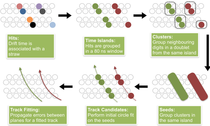
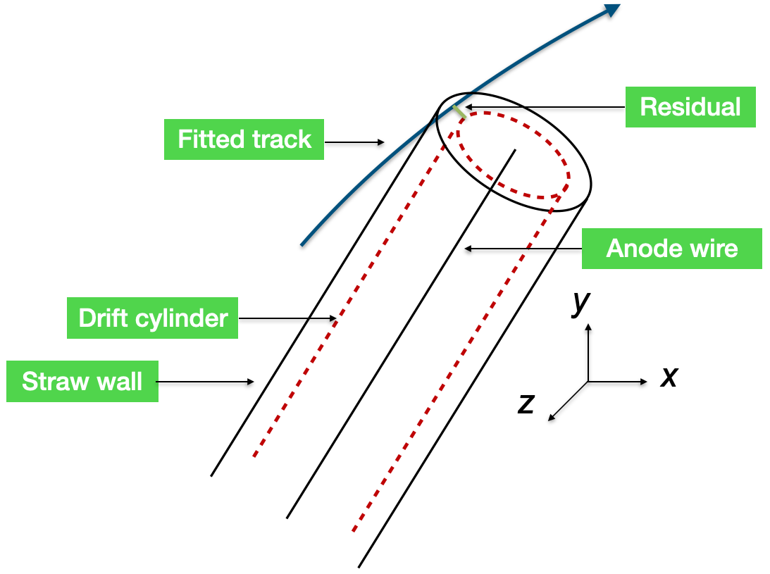
The full tracking algorithm is schematically represented in Figure 5.12, while the formation of a residual between the measurement (i.e. drift circle) and the prediction (i.e. fitted track) is depicted in Figure 5.13.
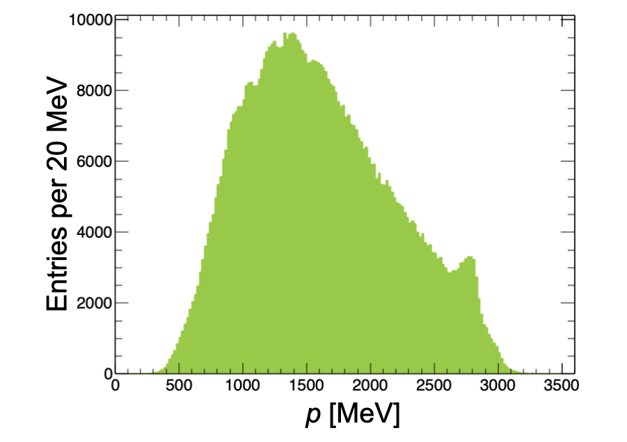
The DCA resolution of hits within the straws is approximately to [66], which surpasses the design goal of . Similarly, a momentum resolution was determined to be at [66], which corresponds to MeV for the mid-momentum tracks, and is in-line with the design goal. The distribution of measured track momenta is shown in Figure 5.14.
5.3.5 Track extrapolation
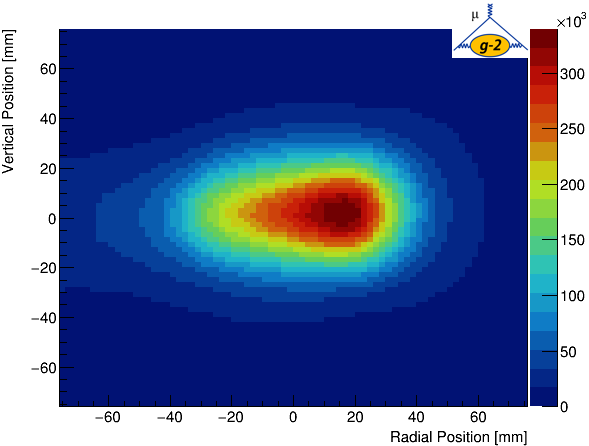
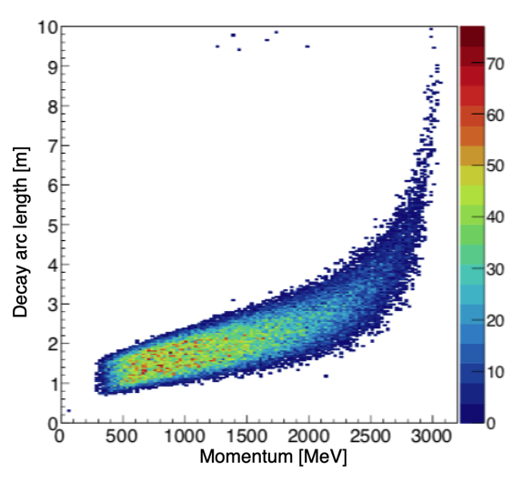
The track extrapolation framework was developed by S. Charity [68]. The fitted tracks are extrapolated back to the most probable muon decay point, as shown in Figure 5.15, using a Runge-Kutta [69] algorithm that propagates the tracks through the varying magnetic field, until the point of radial tangency is reached. The extrapolated tracks are used to measure the muon beam profile, as shown in Figure 5.16a, as well as to calculate the decay arc length, as shown in Figure 5.16b where it is clear that higher momentum tracks originate further away from the detector.

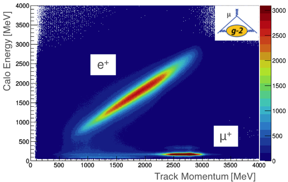
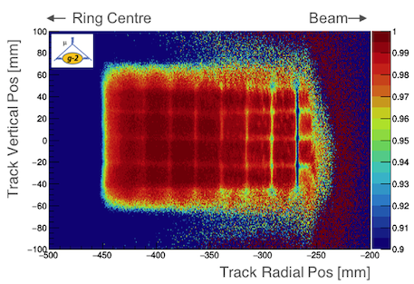
The tracks can also be extrapolated forward to the calorimeter, enabling particle identification, as shown in Figure 5.17a, as well as to investigate the efficiency of matched calorimeter clusters and tracks, as shown in Figure 5.17b. The efficiency decreases in the gaps between the crystals where a \saylost-muon might split its small energy deposition between the two crystals, neither of which goes above the threshold. The data in Figure 5.17b contain early times in the fill (< ), so there are more \saylost-muons, which artificially lowers the efficiency, but brings out the crystal structure (c.f. Figure 3.16). Matching via can also be used to independently monitor the calorimeter gain, and identify the rate of pileup in the calorimeter.
5.3.6 Track quality cuts
Analogous to the data quality control described in Section 3.8.1, the track reconstruction has its own set of criteria to define the quality of a track. These criteria [70] are then used to define a sample of tracks appropriate for a particular analysis. Of particular interest to the analysis in this thesis are the cuts imposing:
-
•
Extrapolated track did not pass through a significant amount of material (e.g. the wall of a vacuum chamber)
-
•
Track passed through at least 12 straws
-
•
Track has a good fit quality with a
Imposing these and other criteria remove of the tracks, which is an acceptable reduction in statistics given the gain in the data quality.
5.3.7 Magnetic field convolution
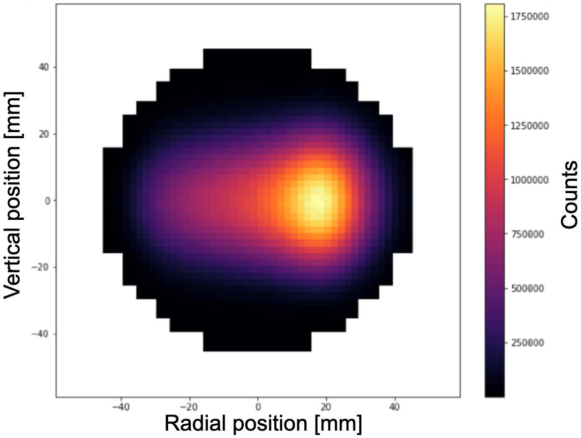
The magnetic field (Figure 3.15) measured by the trolley is convoluted with the beam profile (Figure 5.16a) measured by the trackers to find the average field, , experienced by the muons before decay. Additionally, the calorimeter acceptance (i.e. a fraction of events where a positron is detected by the calorimeters) must be taken into account to estimate the distribution of the muons that are used in the analysis. An example of the acceptance-corrected beam profile is shown in Figure 5.18.
5.3.8 Tracker calibration and efficiency
The track-reconstruction efficiency is defined as the fraction of recorded hits that are associated with tracks. The work to improve the tracking efficiency is ongoing and has so far been able to improve it by a factor of four [72]. Several factors determine the efficiency including the efficacy of the time-island and clustering algorithms (see Figure 5.12), the time-to-distance calibration, the efficacy of making the correct LR assignment, and the alignment of the detectors.
The alignment is an important aspect in improving both the track-reconstruction efficiency and the tracker resolution, with implications for reducing the uncertainty in the tracker-based analysis (see Chapter 9) and the EDM analysis (see Chapter 10). The alignment is discussed in detail, and the results of the alignment procedure presented, in Chapters 6, 7 and 8.
Chapter 6 Systematic contribution of the alignment to the beam extrapolation
6.1 Introduction
A precise calibration of the tracking detector is required to reduce the systematic uncertainty on the measurement and improve the sensitivity to a muon EDM. The calibrations are the time-to-distance relationship and the alignment. The alignment has two components: internal and global. The internal alignment considers the positions of the tracking modules within a station, while the global alignment considers the absolute position of the station relative to the rest of the experiment. The internal position of the tracking modules must be known to a high level of precision. Therefore, a physics-level (i.e. track-based) alignment was implemented with data from Run-1 using the Millepede-II framework [73]. The global alignment was implemented using laser survey measurements of the tracking station chambers. The results and methodology of the global and internal alignments are presented in Chapter 7.
It is imperative, for the beam measurements made with the tracking detectors, to have an estimate of the systematic uncertainty that comes from an internally misaligned detector. One way to produce such an estimate is to add sets of known misalignment offsets to the positions of the tracker modules and reconstruct data with these offsets. A comparison can then be performed between the nominal case and a case with the added offsets.
6.2 Methodology
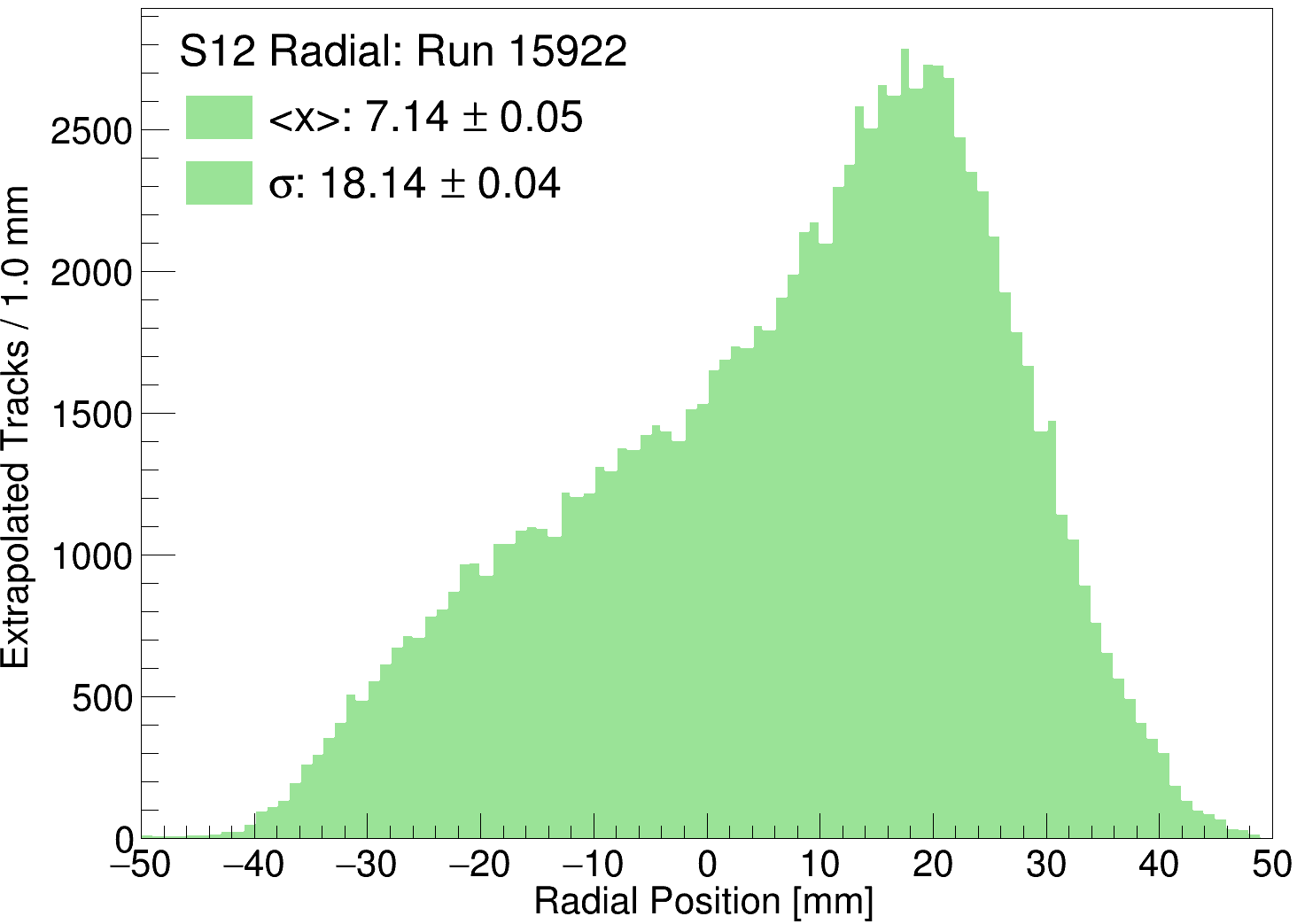
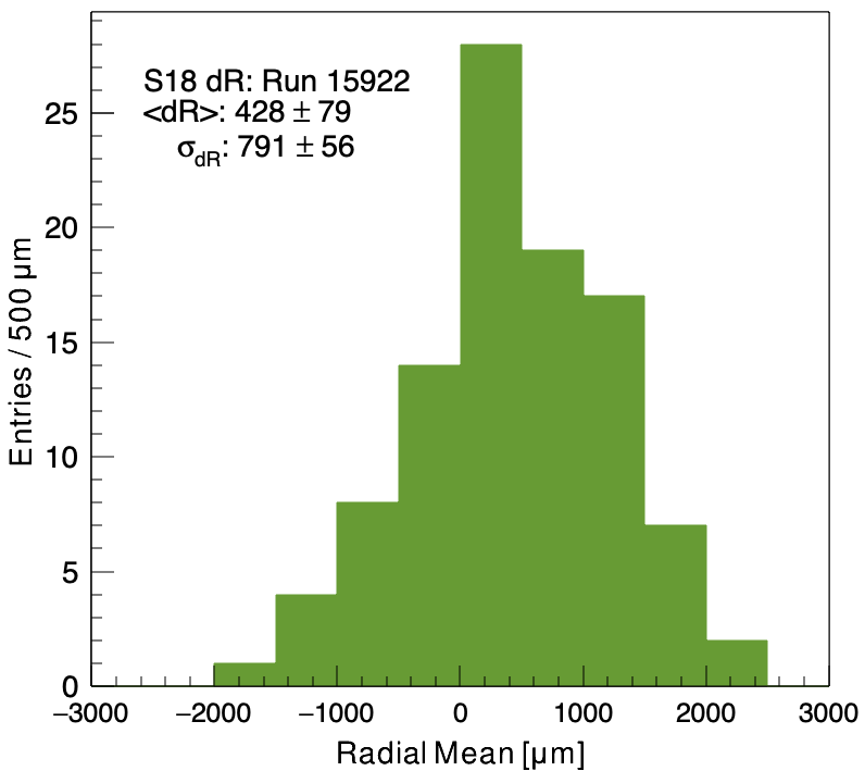
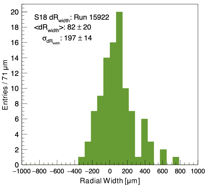
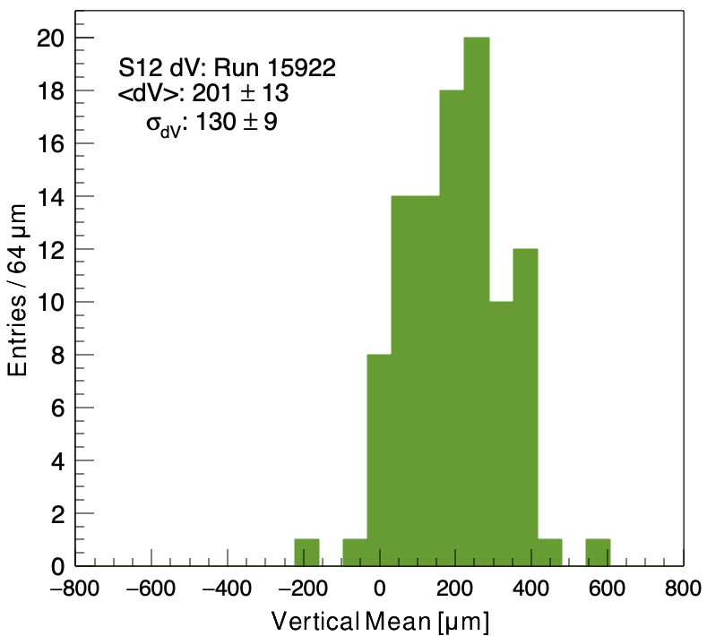
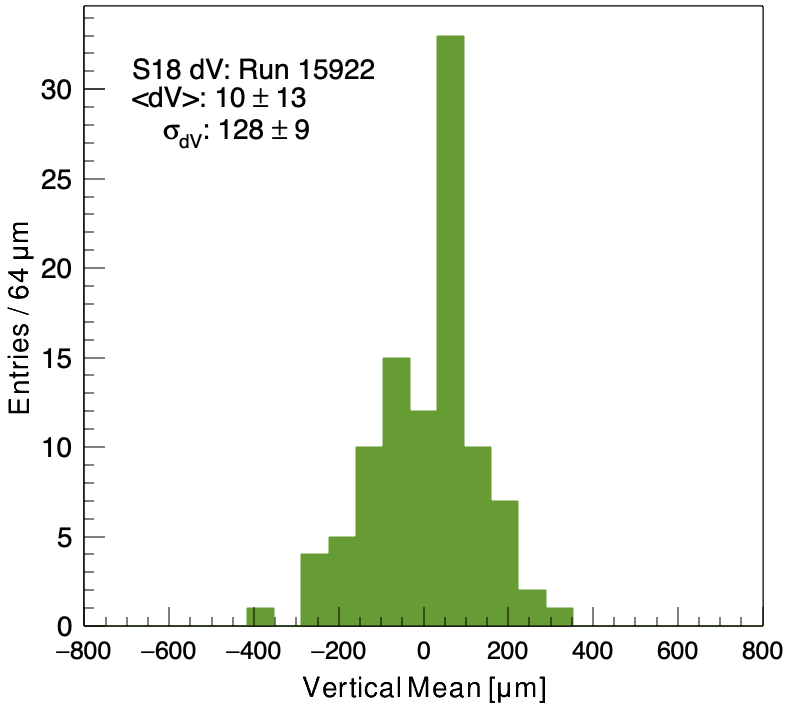
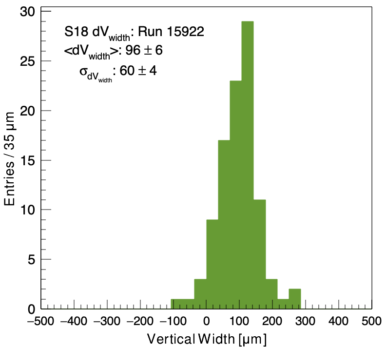
The focus of this study was to quantify the effect that the internal misalignments have on the radial and vertical estimate of the beam’s position. The chosen run (nominal case) for this study was run 15922 (22 April 2018) that contained one hour of data, and the nominal extrapolated radial and vertical beam means and widths for both stations are shown in Figure 6.1.


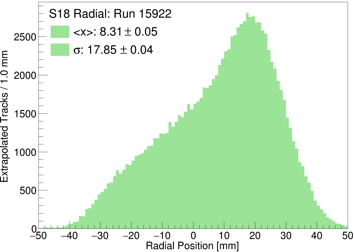
All extrapolations were done after applying the track quality cuts. Additionally, a further cut removing tracks that extrapolate back more than from the beam centre was implemented. This selects tracks that have come from a uniform field region of the storage ring (see Section 3.5). Moreover, only tracks with a time more than were considered. Such tracks have originated from the decay muons that have already undergone scraping (see Section 3.3.3) and have a stable orbit around the ring.
To extract the mean and width of the beam, the vertical distribution was fitted with a Gaussian function between using the method. The radial distribution does not have a Gaussian shape, and so the mean and the width are extracted directly from data. The reason for the non-Gaussian shape of the radial distribution is discussed in Section 3.3.2.
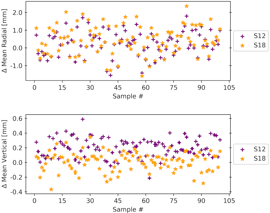
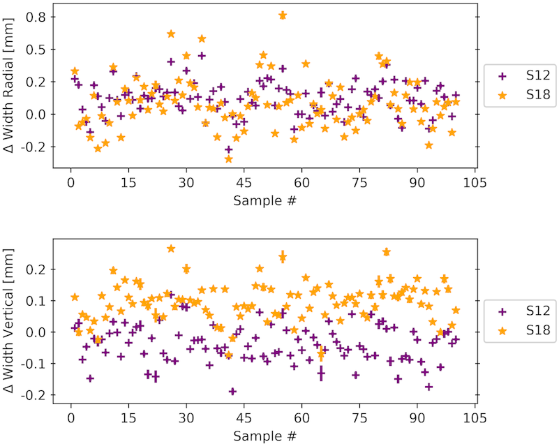
Each of the eight modules in a station was misaligned independently with a misalignment in the range of to . In this study, 100 samples of random offsets were used, as shown in Figure 6.2. In Chapter 7, it is shown that the mean measured misalignment per module is and radially and vertically, respectively. Therefore, the estimated systematic error in this study overestimates internal misalignment contributions to the beam extrapolation.
The task consisted of running the track reconstruction 100 times on a single data run. Each of the two tracker stations yields approximately tracks per run ( one hour), which is reduced to tracks after the track quality cuts are applied, as described in Section 5.3.6.
6.3 Results
The results from the impact of the misalignment on the radial and vertical beam extrapolation are shown in Table 6.1 and Table 6.2, respectively. The extracted quantities of interest are: (1) the difference in the mean extrapolated radial position, , and (2) its standard deviation, , as well as the difference in the width of the beam, , and its standard deviation, . This difference is defined with respect to the nominal value. , extrapolated from run 15922, as shown below for the radial position
| (6.1) |
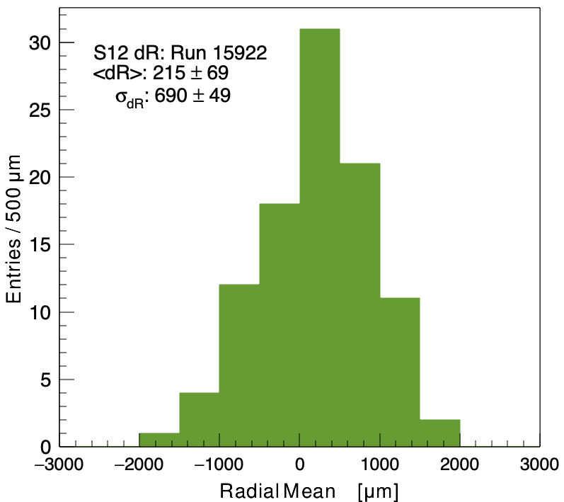
where is one of the randomised samples. The results from Figure 6.2 were accumulated in Figure 6.3 and Figure 6.4, where a comparison between a nominal and a randomised sample was performed according to Equation 6.1. The mean is then extracted from the ensemble as
| (6.2) |
and similarly for , , and , and the four counterpart vertical () quantities.
The uncertainty on the beam extrapolation from the internal misalignment was taken as the mean from the two stations, with the uncertainty computed in quadrature. The final four systematics that were used in propagating the internal alignment contribution to the beam extrapolation are summarised in Table 6.3.

| [] | [] | [] | [] | |
| S12 S18 | 322 105 | 741 74 | 101 24 | 162 17 |

| [] | [] | [] | [] | |
| S12 S18 | 106 18 | 129 13 | 29 8 | 59 6 |
6.4 Internal alignment contribution to the beam extrapolation
The beam extrapolation determines the radial and vertical positions of the muon beam in the storage ring. If the internal misalignment of the tracking detectors is not determined and corrected for, the uncertainty on the mean radial and vertical extrapolated beam positions correspond to 0.741 mm and 0.129 mm, respectively.
The pitch correction (see Section 3.4.1) is given by Equation 3.11. The from Table 6.3 potentially yields a 1.5 ppb uncertainty on the pitch correction arising from the internal misalignment, if the misalignment is not accounted for. Once the misalignment is corrected for, there is a negligible uncertainty in .
| [] | [] | [] | [] |
|---|---|---|---|
| 0.741 | 0.162 | 0.129 | 0.059 |
Chapter 7 Internal alignment of the straw tracking detectors
7.1 Introduction
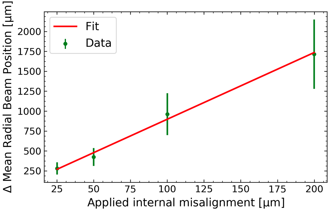
A track-based internal alignment of the two tracking stations was implemented using data from Run-1. A Monte Carlo simulation was also developed to understand how the detector geometry affects how well the alignment can be determined, as well as to test the alignment procedure itself. A high-precision internal alignment of the tracking system is motivated by the need to minimise the uncertainty on the extrapolated beam position. This is illustrated in Figure 7.1, which highlights that even a relatively small-scale misalignment can have a large impact on the extrapolated radial beam position. Additionally, a precise alignment is essential for performing a search for the muon EDM, as described in Section 10.2. Broadly speaking, an internal misalignment of an element of a tracking detector results in a residual between a hit position (e.g. DCA of a hit to a wire) and the fitted track. This residual arises from the fact that the assumed detector position, used in the fitting of the track, is not the actual position of that detector. The alignment procedure aims to establish the corrections to the assumed detector position, and hence, minimise the residuals.
This chapter describes the internal alignment procedures. Section 7.2 describes the chosen framework for the alignment, as well as the general methodology of the internal alignment of a straw tracking detector. Section 7.3 describes the integrity tests of the alignment procedure in a simplified 2D case with straight tracks. Section 7.4 describes the results of the alignment using the full 3D geometry of the real tracking system in an inhomogeneous magnetic dipole field with curved tracks. At each stage, a thorough comparison was made between simulation, data, and where available, analytical predictions. Finally, in Section 7.5 alignment results with data are presented. An overview of the global (external) alignment, which established an absolute position of the tracker stations relative to the rest of the experiment, is described in Appendix A.
7.2 Alignment methodology
The chosen alignment framework was Millepede-II [74], which simultaneously fits many parameters describing the detector geometry and the input data. The framework accounts for the correlations between different alignment elements. This framework is widely used in particle physics: the inner tracker of LHCb [75], and the Belle II [76] vertex detector have both been aligned using Millepede-II. Moreover, a track-based alignment with 50,000 parameters was successfully implemented by CMS [77, 78]. Outside of particle physics, Millepede-II has been used in medical physics for the alignment of Positron Emission Tomography Scanners [79].
The alignment is essentially a least squares regression (LSR) with a large number of parameters. These parameters can be divided into two classes: global and local parameters. Global parameters (i.e. alignment parameters or geometry parameters) affect all tracks (e.g. the radial position of a detector). Local parameters (i.e. track parameters) are associated with individual fitted tracks. For example, a straight line-fit in 2D has two local parameters: a slope and an intercept. Millepede-II performs a LSR, using both global and local parameters, minimising a linearised function of a sum of residuals. A residual, , is defined as the difference between a fitted (predicted) position, , and a measured hit position, , as follows
| (7.1) |
where the fitted track is described by some parametrisation. This is demonstrated in Figure 7.2.

This parametrisation can be written in terms of the aforementioned global, , and local, parameters, and the dependence of these parameters on the residual is
| (7.2) |
where is the fit parametrisation, and subscript defines the association of the local parameters to a particular track. The of many residuals from a single track is given by
| (7.3) |
where is the estimate of the uncertainty in the hit position. The total for many tracks is then
| (7.4) |
A function is then minimised with respect to a variation of the global and local parameters
| (7.5) |
where and are the initial geometry and track parameters, respectively. The corrections to the global parameters, , which minimise , are added to the assumed geometry of the detector to improve the relative alignment and the overall quality of the fitted tracks.
7.2.1 Generalisation of the alignment methods
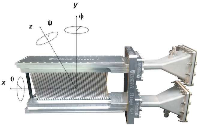
The alignment parameter basis, , is defined by six degrees of freedom (DoF) in the Euclidean 3D space, as shown in Figure 7.3,
| (7.6) |
where , and are the Euler angles. These DoF describe three translations and three rotations of a detector.
In the minimisation from Equation 7.5, a vector containing the derivatives of the residuals with respect to the alignment parameters, , is used. The individual derivatives depend on the functional form of the residual in Equation 7.2.
A line in 3D can be parametrised with a variable parameter as follows
| (7.7) |
as one needs only four parameters to specify a line in 3D. Assuming the track is not parallel to the plane, as will be the case for all the tracks of interest in this study, the parametrised track equations is
| (7.8) |
This yields directly the four local parameters
| (7.9) |
where the two intercept points and are at , and two slopes , where , are given by
| (7.10) |
where is the momentum in the direction, and is the corresponding angle. Therefore, the vector containing derivatives of the residuals with respect to the fitted track parameters is given by
| (7.11) |
7.2.2 Coordinate system transformations
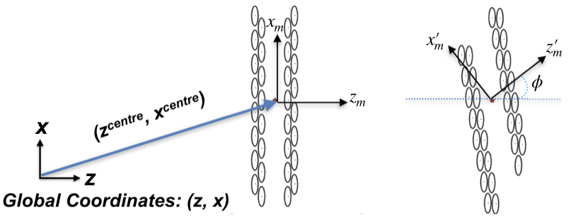
The coordinate systems used in the alignment are defined below. It is important to note, that due to the geometry of the straw tracker, the alignment is not sensitive to shifts in the direction, the \saybeam direction, and corrections to translations along will not be derived. The alignment corrections for the other global parameters will be derived directly in the station coordinate system. The coordinate systems are:
1) Global (ring) coordinates .
2) Detector (tracker station) coordinates , with the origin of at the centre of the first of the eight modules.
3) Local (tracker module) coordinates , with the origin of at the centre of rotation of a module.
In the case of 3D translations and rotations, a tracker module is connected to the station coordinate system via the relation
| (7.12) |
where is the module position in the station coordinates, and is the 3D rotation matrix (see Equation B.35). An example of such a transformation in 2D is illustrated in Figure 7.4. With the above definition, the alignment corrections, as given in the tracker station frame, can be represented by
| (7.13) |
where corrections for translations, , and rotations, form the alignment parameter vector described in Equation 7.6.
7.2.3 Parameter optimisation methods
The number of all the parameters in Equation 7.5 could be large, hence, the differential equation is first linearised, to allow for a subsequent matrix inversion, and then reorganised into a block matrix equation [80] of the form
| (7.14) |
where is a matrix containing the connection between the local and global parameters, is the correction vector (for global parameters), and a vector of the normal equations [73]. Hence, a matrix inversion, whose dimension is given by the number of global and local parameters, is necessary to obtain the corrections to the global parameters that simultaneously minimises the . However, the size of the matrix can be reduced, as the derivatives with respect to the global parameters are the only parameters of interest, as contained in the sub-matrix
| (7.15) |
Advanced matrix algebra techniques and the assumption that is invertible are used [74] to remove the unnecessary parameters, such that only the inverse of is needed to establish the corrections to the alignment parameters.
7.2.4 Alignment software framework
An alignment software module, written in C++, has been developed as part of the art software framework [50]. This module is run after the track-fitting (see Section 5.3), and it can be used on data or simulation. The geometry is defined at the tracking stage and is passed to the alignment module, which also calculates the residuals of the selected tracks, as well as computes the local and global derivatives. A C++ module (Mille) is provided [74] to write this information into a binary file which is passed to PEDE (a Fortran executable), which performs a simultaneous fit via the matrix inversion described above. The alignment module is also responsible for writing a constraints file (specifying the redundant DoF), and a steering file (specifying the mathematical methods used by PEDE). The final outputs of the PEDE algorithm are labels and the corresponding fitted values of the global parameters and their errors. The components of the algorithm are shown in Figure 7.5.
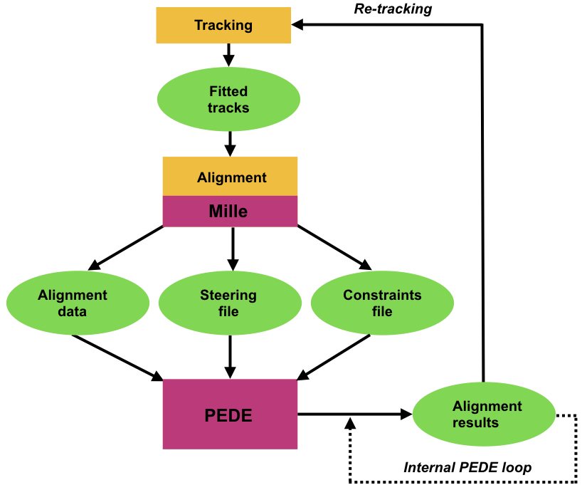
Given that the number of total alignment parameters for the tracking detector is relatively small (), then the PEDE inversion method with 10 iterations (internal PEDE loop) and a 0.01 convergence rate on in Equation 7.5 is adequate for the minimisation of . The advantage of this inversion method is that it also provides uncertainties on the corrections to the global parameters. The memory space requirement for the matrix inversion and the execution time are acceptable. For an entire run of data with tracks the execution time of PEDE is and the memory footprint is below MB. The initial choice of convergence rate and number of iterations is empirical and is comparable to the values deployed by Millepede-II developers [81]. The final choice of steering and constraints methods is discussed in more detail in Appendix C.
7.3 Alignment validation in simulation
To validate the alignment software independently of the art framework, a standalone framework was developed [5]. This framework, written in C++ and Python, interfaces with Millepede-II, and also incorporates a simplified detector geometry. It generates straight tracks and reconstructs them in 2D. This is described in Section 7.3.1. Section 7.3.2 describes the progression to a 3D geometry with a simplified art tracking chain with straight tracks, without a magnetic field and no detector material. The next implementation using a uniform magnetic field, curved tracks, and detector material is described in Section 7.3.3. The final implementation with an inhomogeneous magnetic field in the full simulation is presented in Section 7.3.5.
7.3.1 2D geometry
Translational and rotational misalignments (as defined in Figure 7.3) in the middle modules were considered, with the first and the last modules fixed with no misalignment. An outline of the standalone simulation and fitting procedure to validate and test the alignment using four tracker modules (with four layers per module) with straight tracks in 2D is given below:
-
1.
Define the ideal geometry (i.e. assumed straw coordinates).
-
2.
Define the misaligned geometry (i.e. actual (truth) straw coordinates).
-
3.
Generate straight tracks of the form through the misaligned geometry.
-
4.
Calculate the measurement DCA, , from the truth track and a straw hit in each layer (see Figure 7.2).
-
5.
Smear the DCA by the detector resolution, .
-
6.
Reconstruct the DCA in the ideal geometry.
-
7.
Fit a line to the reconstructed hit points (or reconstructed drift circles, as described in the next section), and calculate the residual between the fit and the hit point.
-
8.
Pass residuals, as well as global and local derivatives, to PEDE to perform the minimisation of the residuals using the matrix inversion method.
7.3.1.1 Translational misalignment in with a straight line-fit
In the simple 2D geometry it is possible to define three distinct manifestations of misalignment:
1) is the characteristic misalignment, which is specific for each individual straw layer . is set in the simulation as the truth misalignment. The aim of the alignment procedure is to then recover this input misalignment as close as possible to the truth. The recovered misalignment is called the reconstructed misalignment.
2) is the overall misalignment given by
| (7.16) |
where is the total number of detector layers.
3) is the shear misalignment which corresponds to the mean of the residual, , for a layer
| (7.17) |
where is the total number of tracks. With these definition, is then given by
| (7.18) |
where is the horizontal position (along the beam) of a layer . The standard deviation (SD) for a distribution of residuals in layer is given by
| (7.19) |
Using the above equations, it is possible to show (see Section B.1) that the expected mean for a given set of characteristic misalignments is given by
| (7.20) |
where the summation is over all layers. For a straight track-fit in 2D, there are two redundant DoF, which are removed from the above equation. Any misalignment will shift the mean of the residuals for the misaligned and the non-misaligned modules. Moreover, for a non-misaligned scenario, the expected SD of the residuals at layer is given by
| (7.21) |
The analytically derived equations for , and are compared to the predictions from the simulation in Figures 7.6 to 7.7, and are seen to agree excellently.
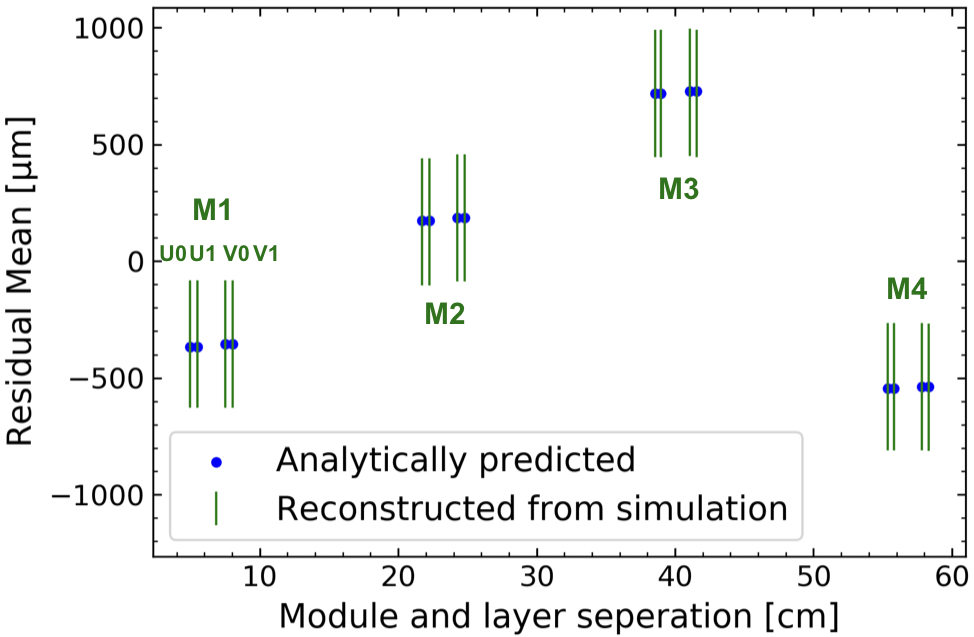
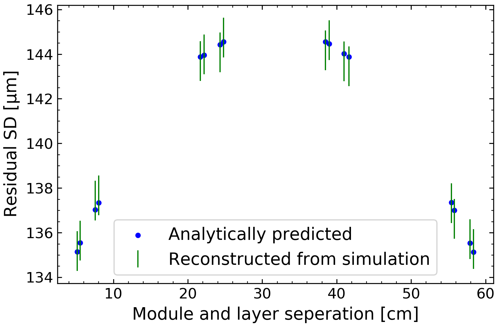
Having established the integrity of the analytical predictions, PEDE was then used to study the number of tracks required for the alignment parameters to converge on acceptable values. The inputs to PEDE are summarised below. The residual was defined according to Equation 7.2
| (7.22) |
where is the closest vertical distance to a wire, in this simplified case. A constant detector resolution (i.e. hit smearing) was defined for all hits of
| (7.23) |
Two local parameters defining the slope () and intercept () of the track were used and only a single global (alignment) parameter () was used such that the derivatives are:
| (7.24) |
Two modules were misaligned by and , and the difference between the known input misalignment and that determined from PEDE is plotted in Figure 7.8 as a function of the number of tracks. It is seen that acceptable alignment parameters are determined after tracks.

7.3.1.2 Translational misalignment in with a circle-fit
In the previous study, a simplified straight line-fit to the hit positions was used. In reality this is not possible, due to the so-called LR ambiguity (see Section 5.3.3), and the fact that the measurement in the straw is a drift circle (see Section 5.3.1). In the case of a misalignment, the LR ambiguity can cause the alignment minimisation to fail. For this reason, only hits with greater than are used. Moreover, this requirement is also necessary to avoid a discontinuity in the residual derivative (see Equation B.16).
A simulation framework incorporating 2D misalignments using a circle-fit was implemented. An example of five generated tracks in four tracker modules is shown in Figure 7.9. Due to the empirical nature of the circle-fit (which is performed by finding the minima numerically), the exact analytical predictions for , , and cannot be derived. However, other tools exist to check the solutions, as described in the rest of this chapter.
The inputs to PEDE in the case of a circle-fit using straight tracks are given below. In the circle-fit, the closest point on the drift circle to the track is determined first, with the residual, , given by
| (7.25) |
with two local derivatives, and given in Equations B.16 and B.17, and a single global derivative
| (7.26) |

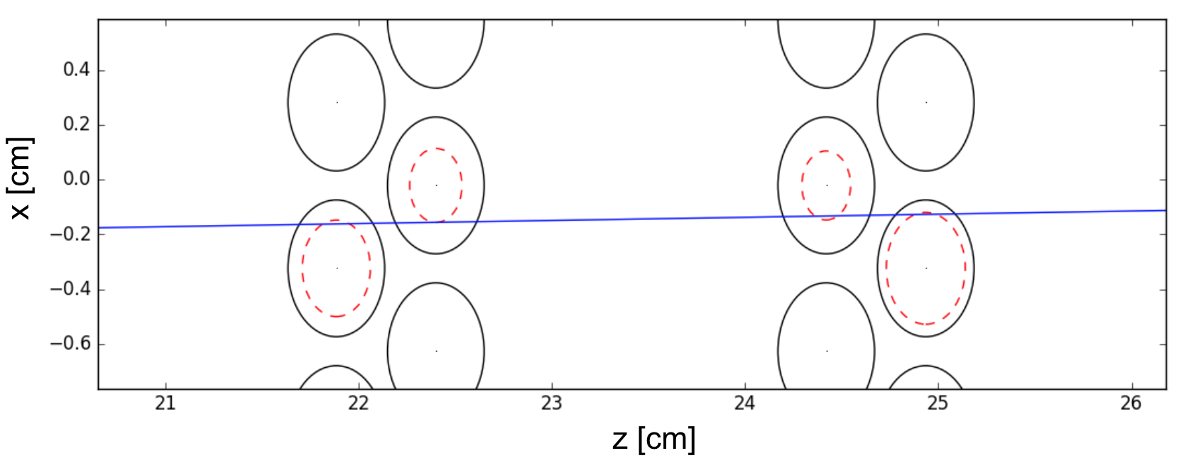
A simple misalignment of M3 was analysed. The improvement in the distribution of residuals is apparent as seen in Figure 7.10 and Figure 7.11; with the final figure-of-merit for alignment given in Figure 7.12. To obtain the results after the alignment, the predicted global parameters by PEDE were used as the correctional offsets to the assumed geometry.
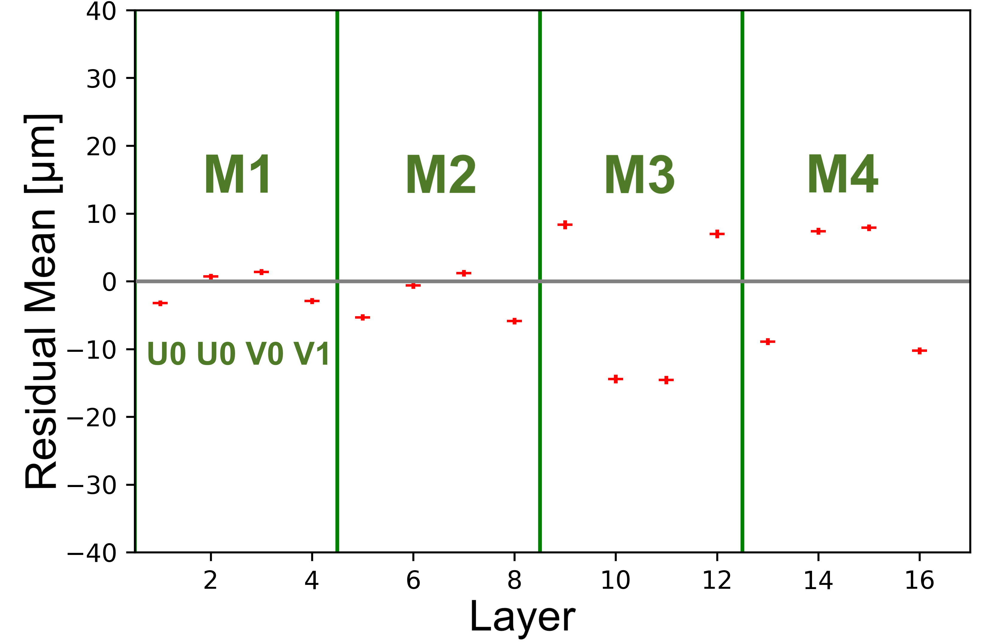
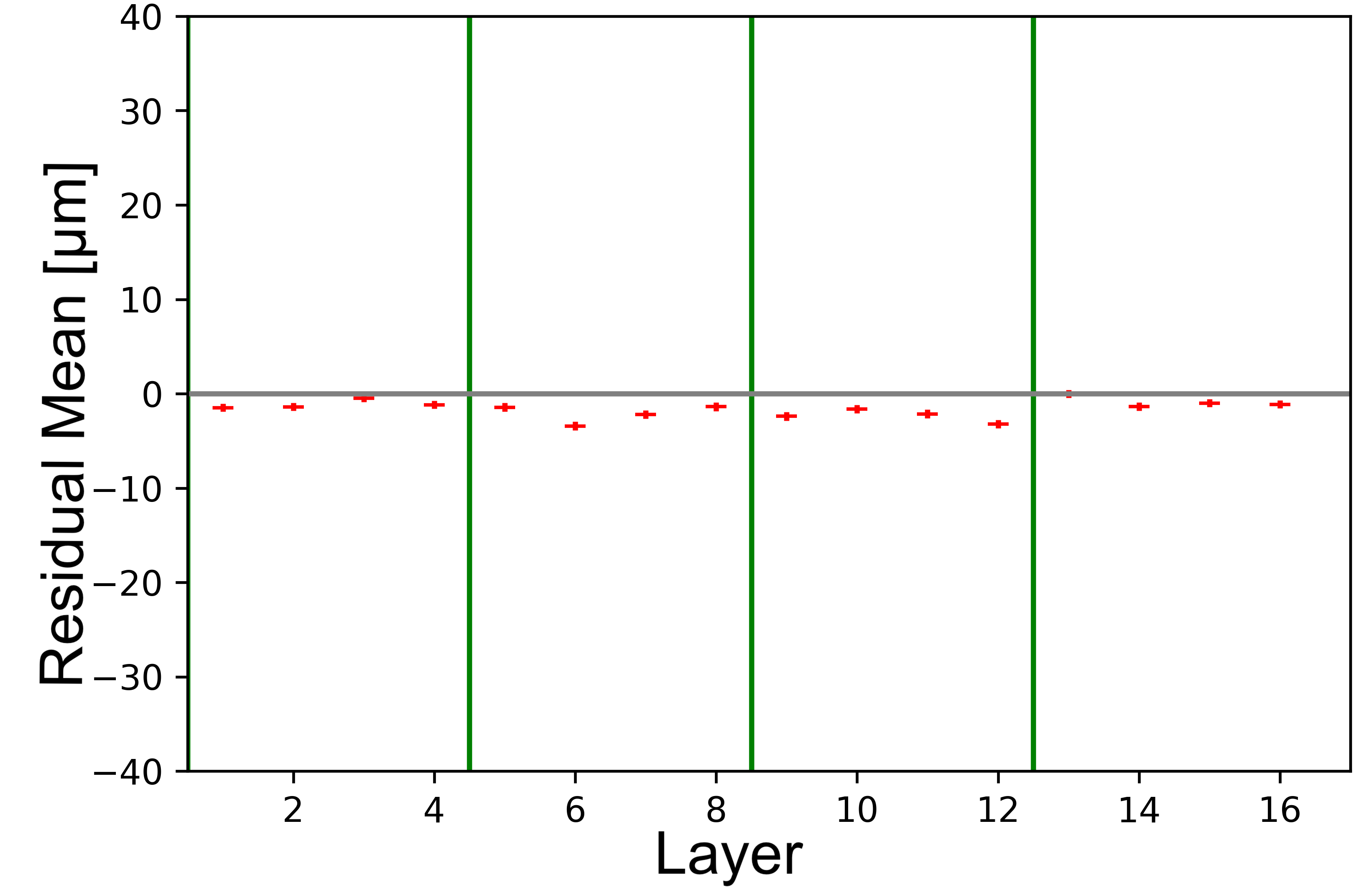

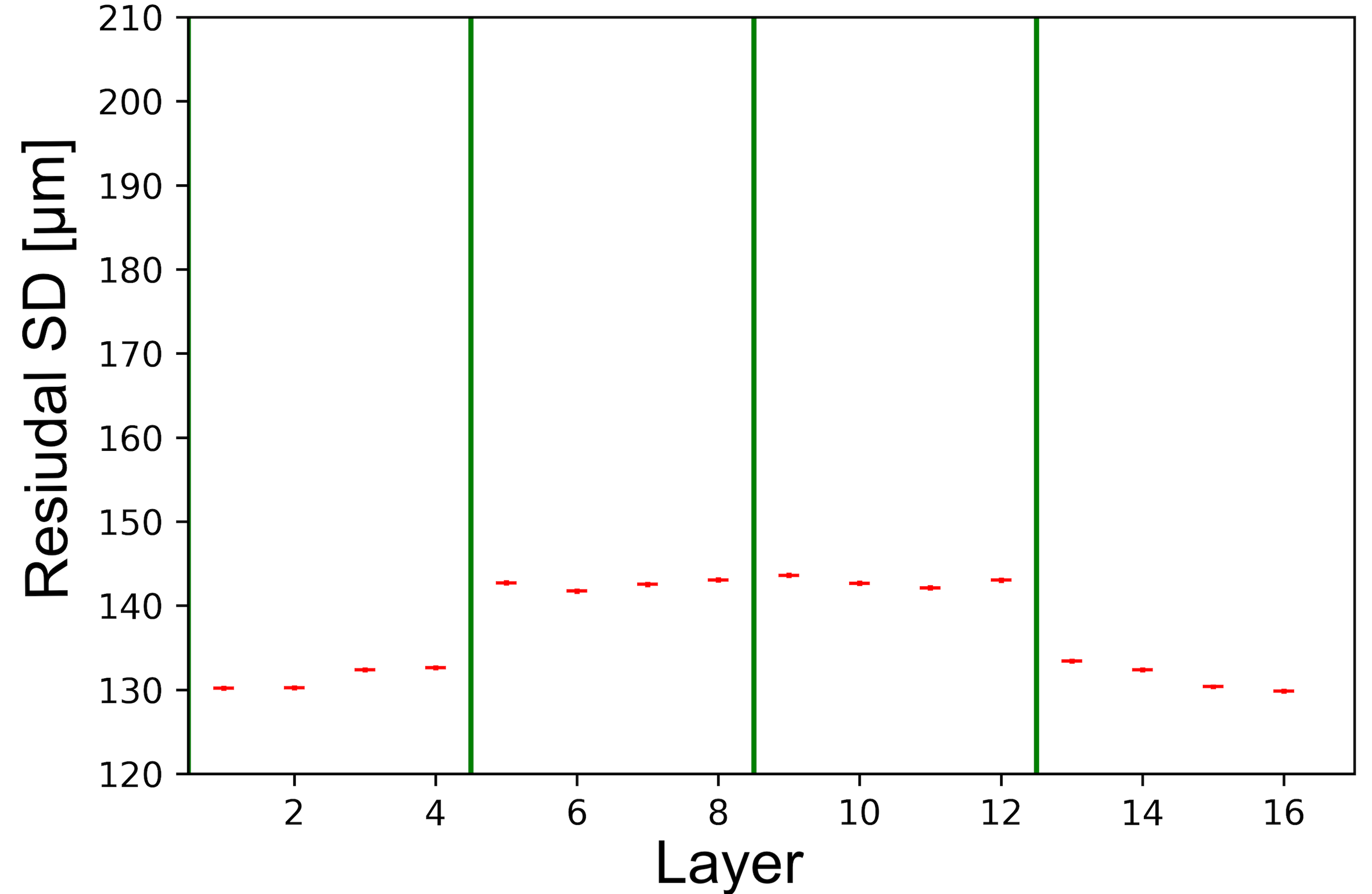


7.3.1.3 Translational and Rotational misalignment in the plane with a circle-fit
The aim of this section is to evaluate the circle-fit residuals with a misalignment induced by an anticlockwise rotation () in the plane through the detector centre.
There are three coordinate systems defining straw positions (see Figure 7.4):
1) Global coordinates (, ) relative to the \sayglobal (0, 0). The derivatives of interest are given in these coordinates.
2) Local module coordinates (, ) in the un-rotated frame relative to the centre of rotation of a module, which is given by (, ).
3) Local module coordinates (, ) in the rotated frame. Such that, the centre of rotation (, ) = (, ) = (0,0), in the local coordinates.
With and transformations, the action of an anticlockwise rotation is given by the reduced 2D form of the rotation matrix (see Equation B.35), and the equation for the residual is derived in Section B.2.
The result of the PEDE minimisation for modules 2 and 3 in and is shown in Figure 7.13. Again, the correct alignment is realised after tracks are fitted.
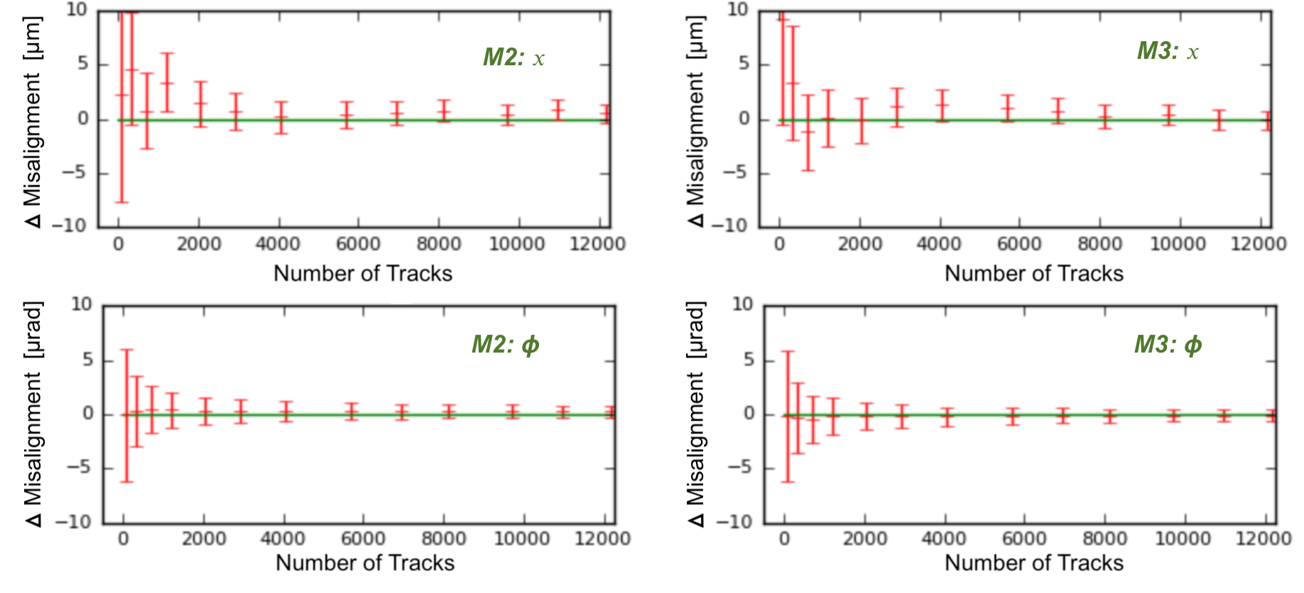
7.3.2 3D geometry
In this section we will consider the case of a misalignment in 3D, with the tracker geometry coming from art. The residual of interest, between the reconstructed track through the detector and the \saydrift cylinder (as shown in Figure 5.13), is now a function of the DCA between two skew lines: the track and the straw wire. The assumption of the two lines being non-parallel will hold for all physical tracks of interest; the track and the wire can intersect, however. The visualisation of this case study with four modules is given in Figure 7.14. In this instance the misalignment is radial and the is vertical.

The DCA between the track and the wire is given by
| (7.27) |
where W and T are the points of closest approach between the wire and the track, respectively – as indicated by the ′ notation on the coordinates. The vector is perpendicular to both the wire and the track, as shown in Figure 7.15.
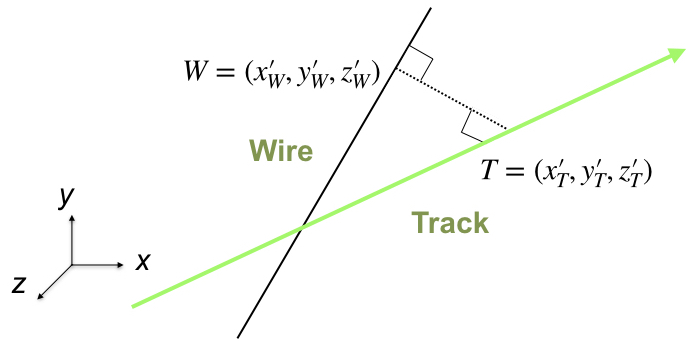
In order to form the required derivatives with respect to local and global parameters, one needs the functional form of the DCA expressed in terms of the reconstructed track parameters and the wire parameters. These derivations are given in Section B.3.
There are three possible rotations (see Figure 7.3) around the centre of the tracker module. A rotation around the -axis is the same as considered previously in Equation B.23, but needs to be extended to a 3D geometry. With the constraint that a point along the straw will have the same vertical height () before and after the above rotation, the derivative for the anticlockwise rotation along the -axis given by
| (7.28) |
and similarly for the other two rotations, as shown in Section B.3.
7.3.3 Uniform field
A uniform field throughout the tracker region of was implemented in the simulation as shown in Figure 7.16.

In a magnetic field, a fifth local parameter can be added to describe the track-curvature, , where
| (7.29) |
and is the momentum of the particle, and the approximation is used to calculate the fifth local derivative, , as derived in Equation B.40.
Results of the radial alignment with eight modules in 3D with curved tracks are shown in Figure 7.17. The non-convergence of the recovered alignment, as compared to the truth misalignment in some modules, is indicative of not constraining the global DoF, as described in Section 7.3.4.
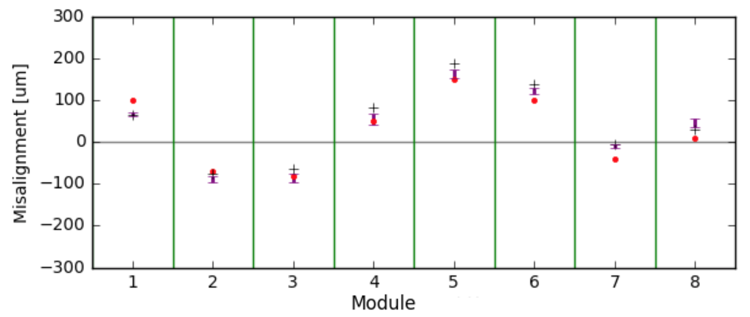
7.3.4 Constraining global parameters
In the particular case of the radial and vertical alignment of the tracking detectors with curved tracks in a magnetic field, constraints to five global DoF are applied. There are two overall translations, radially and vertically, that must sum to 0, and two global rotation angles, also fixed at 0. The global rotation is defined through the centre of the station. This is done to minimise the \saylever-arm effect. The fifth constraint addresses a radial detector curvature (sensor curvature) [82] due to the radially curving tracks in the magnetic field. The constraints can be summarised as follows: the radial constraints equation
| (7.30) |
and the vertical constraints equation
| (7.31) |
where is the centre of the station, and , , and are the curvature, rotation, and translation parameters, respectively. The summary of the steering and constraint inputs to PEDE is given in Appendix C.
The motivation behind constraining the overall translations and rotations is simple: internal alignment should not return the module offsets related to the global movements. The global alignment should independently measure these global movements, as described in Appendix A. The constraint on the radial detector curvature deserves a special mention, as it is essentially a \saylocal minima problem. The internal alignment can place the tracker modules along a curved path, as the residuals will be unchanged. This radial detector curvature, however, will change the measurement of the momentum of the tracks, and the extrapolated beam position. The detector curvature, therefore, must be measured and eliminated by another means, as described in Chapter 8.
7.3.5 Inhomogeneous magnetic field.
Finally, to make the simulation as realistic as possible, the modules were placed in the vacuum chamber as shown in Figure 7.18.
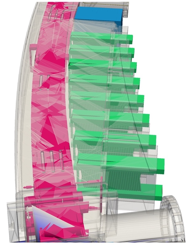
The full experimental simulation framework (gm2ringsim), as described in Section 3.9, is now used. This also adds an additional complication of a radially non-uniform magnetic field in the tracker region as shown in Figure 7.19, and multiple scattering due to the presence of material (e.g. a vacuum chamber).
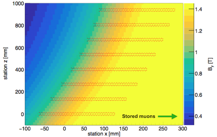
7.3.6 Tracking cuts for alignment
The following cuts were used to select tracks, from simulation or data, to determine the final alignment:
-
•
Maximum layers with multiple hits = 0. Only select tracks that have an unambiguous set of hits in a single straw per layer.
-
•
DCA > . A hit with a small DCA is not used in the alignment. This is required to prevent a residual discontinuity as we cross the LR boundary (Equation B.29-Equation B.32).
-
•
-value > 0.005. Only tracks that have a reasonable fit quality are used.
-
•
Hits > 9. Only tracks that have hits in at least three modules are used.
-
•
> 0.93. Tracks that have large curvature are removed, required by the approximations used in Equation B.40.
7.3.7 Iterative alignment
The process of iterative alignment uses the initial module offsets from PEDE in the subsequent re-tracking. In iteration two onwards, the tracks are formed through a corrected detector geometry, and only small alignment corrections are returned in the subsequent PEDE alignment, as shown in Figure 7.20. The iterative alignment is considered to converge when the returned alignment results agree with a previous iteration to within the PEDE error (few ).
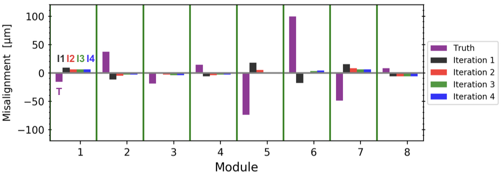
7.4 Alignment results in simulation
The mean values of the residuals per module before and after the alignment are shown in Figure 7.21. The alignment results in both stations after three iterations are shown in Figure 7.22. The improvement in the mean and number of reconstructed tracks as a function of number of iterations is shown in Figure 7.23.


The overall input (i.e. truth) misalignment in station 18 was greater; hence, after the alignment, the improvement in station 18 is more significant than in station 12. The alignment stability was reached, and the alignment convergence was established within and radially and vertically, respectively, in simulation.
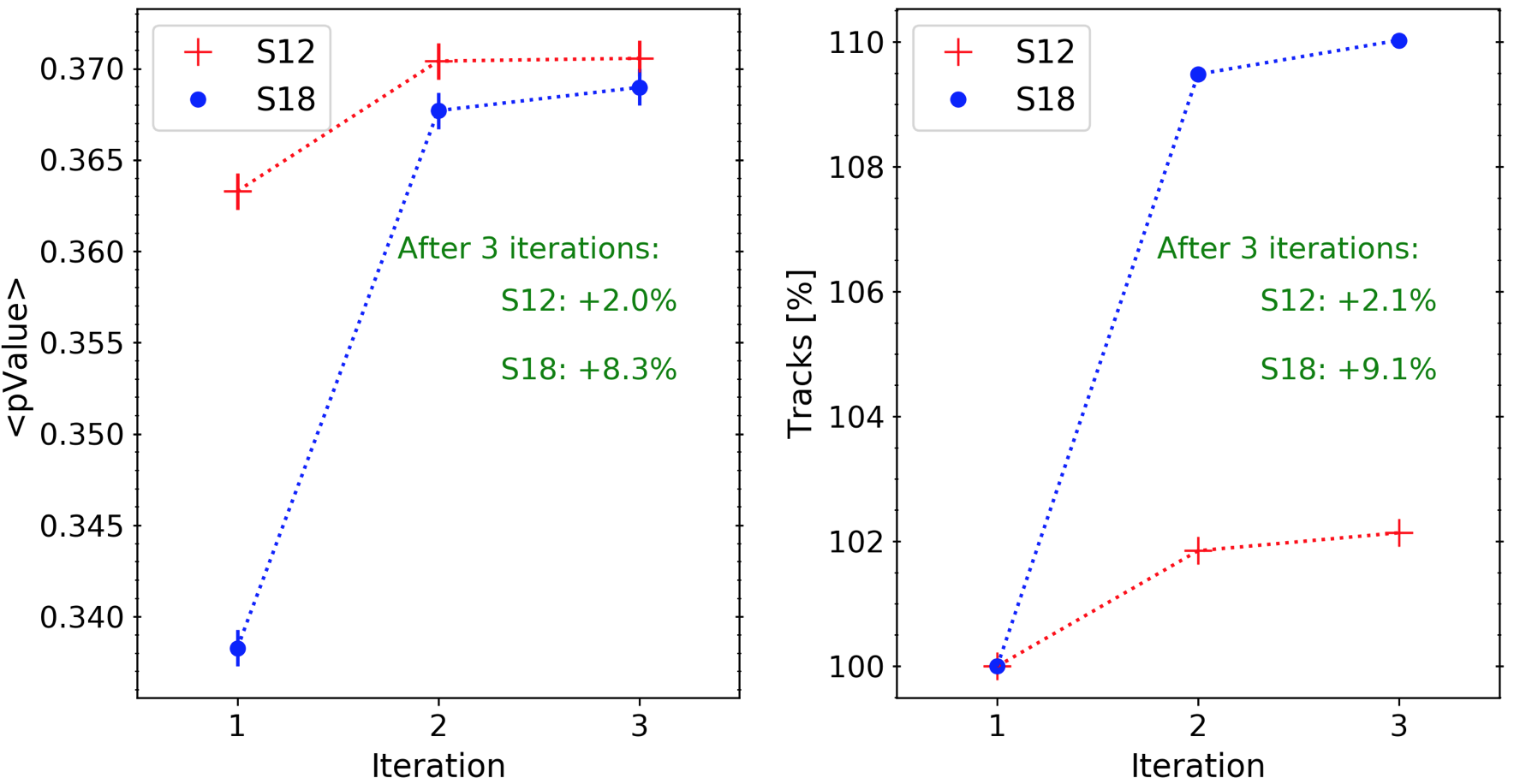
7.5 Alignment results with data
The mean values of the residuals per module before and after the alignment, using run 15922, are shown in Figure 7.24. The alignment results in both stations after three iterations are shown in Figure 7.25. The results were obtained with tracks, and were then used in the track reconstruction.
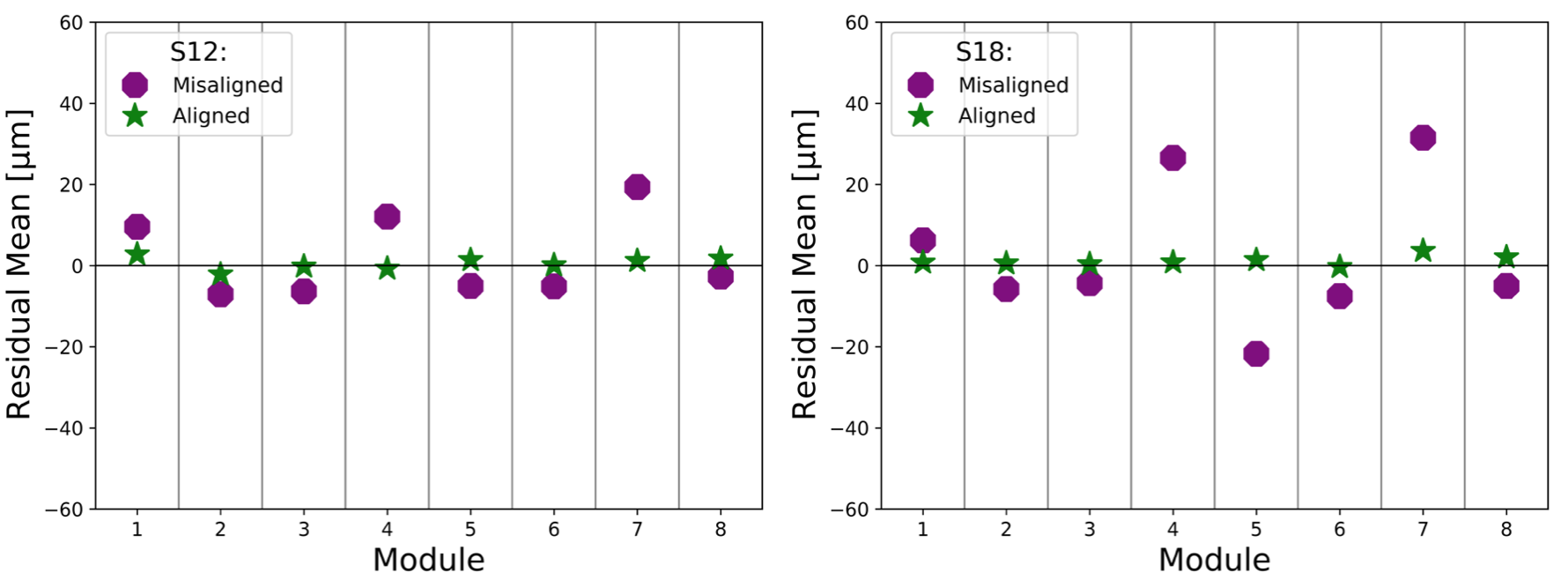
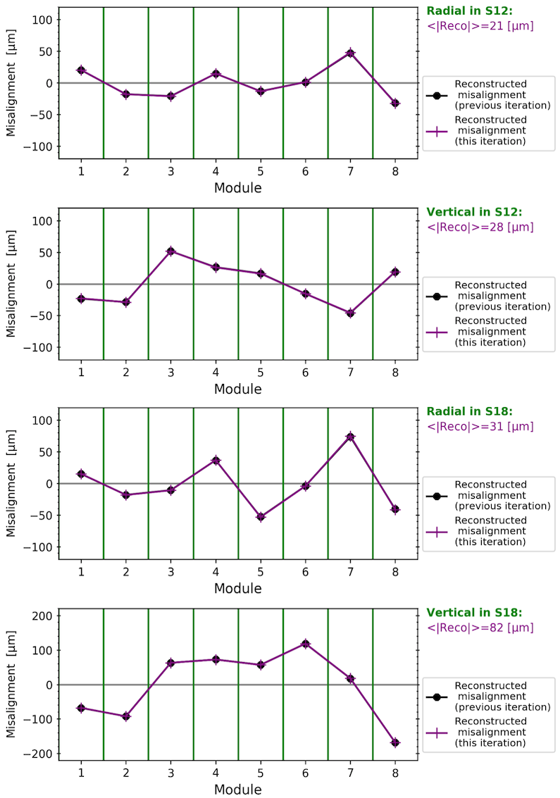
The improvement in the mean and number of reconstructed tracks as a function of number of iterations is shown in Figure 7.26. The change in the distribution of and momentum, as well as in the beam extrapolation are shown in Figure 7.27 and Figure 7.28, respectively.

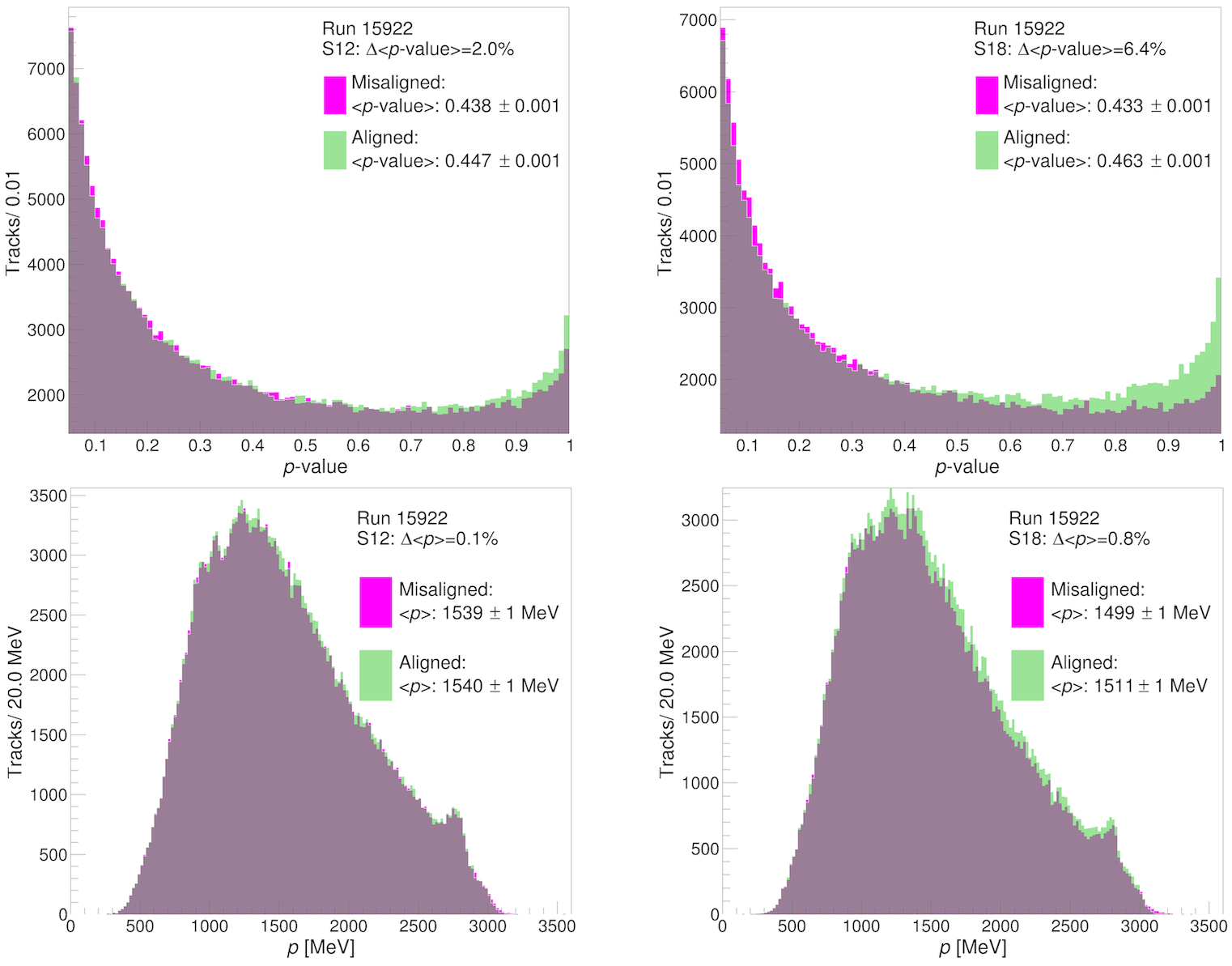
Stations 12 and 18 have a 2.0% and 6.4% improvement in the mean track , respectively. This implies that after the alignment the quality of the reconstructed tracks is higher. Moreover, due to the improved alignment, more tracks are reconstructed from the same hits in station 12 and 18, by 1.5% and 4.5%, respectively.
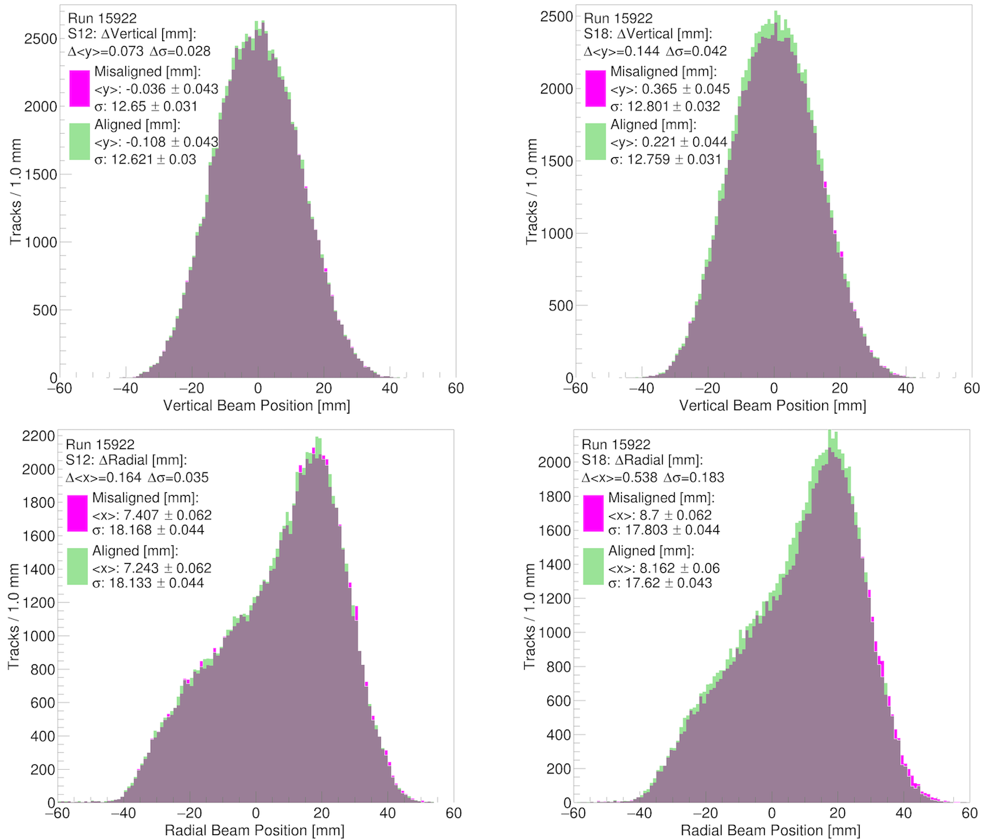
The extrapolated tracks (for ) from stations 12 and 18 have a radial shift towards the centre of the ring of and , respectively. The extrapolated tracks have a vertical shift downwards of and for stations 12 and 18, respectively.
7.5.1 Alignment monitoring system and database
As seen from Figure 7.26, the most significant alignment corrections come after the first iteration. Subsequent iterations yield corrections comparable to the PEDE uncertainty. Hence, an assessment of the alignment stability across all runs is possible, by running the alignment directly on the reconstructed tracks from all runs without an iterative alignment. The radial alignment results per module in station 12 over a 60-hour period (Run-1a dataset) are shown in Figure 7.29.
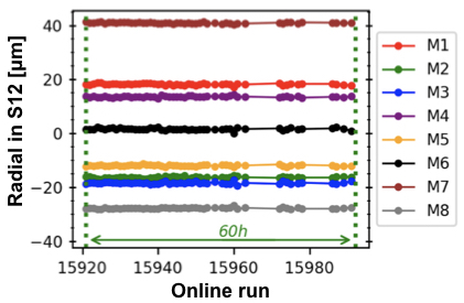
The alignment stability in both stations, radially and vertically, across Run-1 and Run-2 is shown in Figure 7.30.

The change in the internal alignment of the two modules is seen in Figure 7.30: before the start of Run-2 in module 4, and after run 25086 in module 6. These modules were replaced [83] with spare modules, since the existing modules had developed a slightly higher gas leak rate into the storage ring vacuum than the specification. New alignment constants for the replaced modules were derived. The alignment constants were written into a PostgreSQL database, where each set of constants is associated to a given range of runs.
7.5.2 Outlook
The internal alignment, radially and vertically, of the two tracker stations in Run-1 and Run-2 has been successfully determined. Moreover, the alignment manual [3], to monitor the alignment in the future, has been produced. There are, however, a few more activities that are planned to further refine and improve the alignment:
-
•
Scattering target. A placement of a scattering target, as shown in Figure 7.31, in a known position in the storage ring will give a precise location of the starting position of the tracks. This project is being developed by S. Foster [84].
-
•
Internal alignment with rotations. The current tracking algorithm (see Section 5.3) assumes that the tracker planes are parallel to each other. The use of a Kalman filter algorithm, currently in development by A. Luca [85], will allow for rotations of tracker planes, and hence, will improve the alignment.
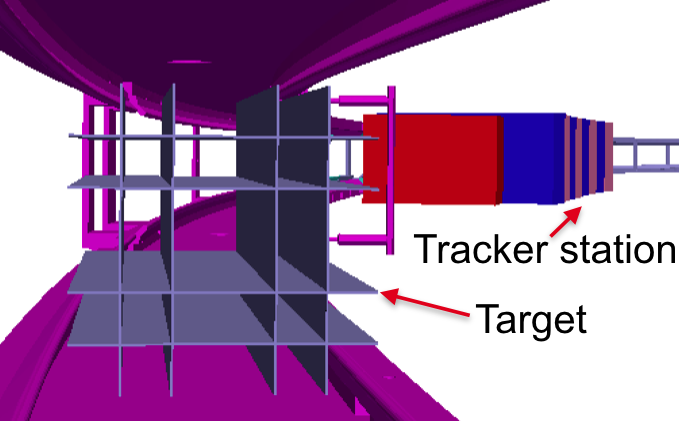
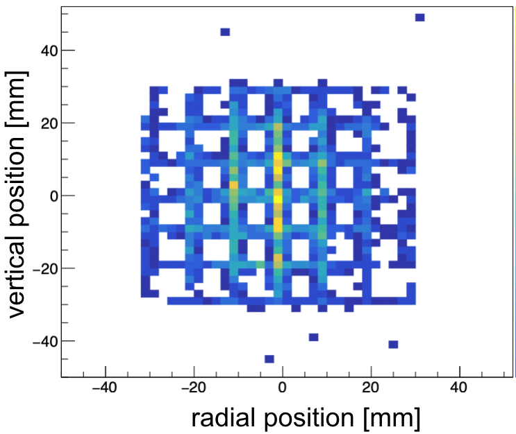
7.5.3 Alignment impact on the systematic uncertainties
7.5.3.1 Pitch correction ()
The beam extrapolation determines the radial and vertical positions of the muon beam in the storage ring. The accuracy of this determination is affected by detector calibrations, such as the alignment. The internal alignment of the tracking detectors is now established, with the uncertainties on the mean and width of the beam given in Table 7.1. In the table, the combined uncertainty, in both stations, from Figure 7.28 was taken.
| [] | [] | [] | [] | |
|---|---|---|---|---|
| S12 S18 | 0.351 | 0.109 | 0.109 | 0.035 |
However, the alignment is now accounted for, as the correct module positions are now used in the track reconstruction. For example, in Chapter 6, the uncertainty on the pitch correction, , from an averaged randomised internal misalignment was estimated to be 1.5 ppb. After the implementation of the internal alignment, this uncertainty was eliminated. This has reduced the total contribution to the uncertainty on the pitch correction from tracking (see Section 3.4.1) from 8.6 ppb to 8.4 ppb.
7.5.3.2 Field convolution ()
The magnetic field is convoluted with the beam profile measured by the tracking detectors to find the average field experienced by the muons before decay, as described in Section 5.3.7. As previously discussed, the measurement of the beam profile from the tracking detectors is affected by the internal alignment. A study of an impact of translations on the extrapolated beam profile from the tracking detectors on the field measurements was performed by Jason Bono and Saskia Charity [71]. Given the scale of translations induced by the alignment in Figure 7.28, it is possible to estimate the corresponding uncertainties on , and hence (see Equation 3.2). The results for both stations are given in Table 7.2, with the average vertical and radial uncertainties on of 3.8 ppb and 0.7 ppb, respectively. After the implementation of the internal alignment, these uncertainties were eliminated. This compares to the overall goal of a 70 ppb uncertainty on the determination of at the end of the experiment’s data taking.
| S12 radial | S18 radial | S12 vertical | S18 vertical |
| 1.5 ppb | 6.1 ppb | 0.4 ppb | 0.9 ppb |
Chapter 8 Detector curvature
8.1 Introduction
A radial curvature in the positions of the tracker modules, as shown in Figure 8.1, changes the measurement of the momentum of the tracks, and the extrapolated beam position. As described in Section 7.3.4, this detector curvature must be measured and constrained by a method that is independent of the internal alignment. One such method is described here, along with the derivations of the tracking systematic uncertainties arising from the curvature.
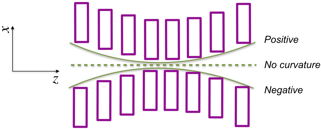
8.2 Impact on alignment and tracking
If the internal alignment is established without constraining for the radial detector curvature, the recovered alignment results will contain an erroneous curvature. Even for a case of no input misalignment in simulation, the absence of the correct constraints will introduce this erroneous curvature, as shown in Figure 8.2.
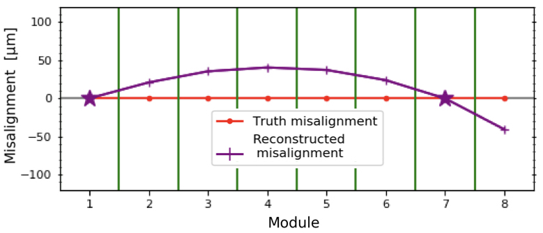
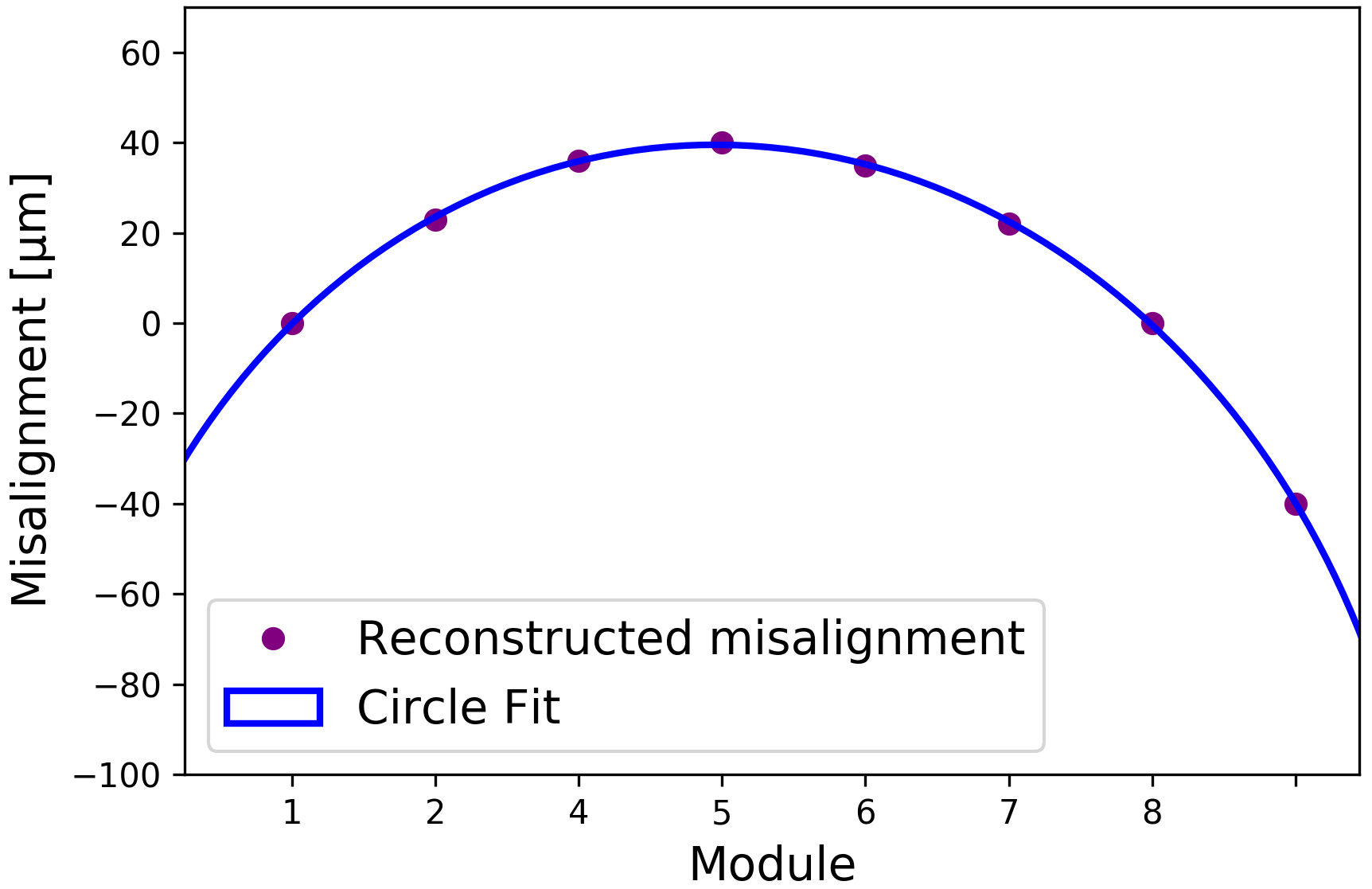
Re-tracking with the modules placed in the suggested position from Figure 8.2 changes the momentum distribution of the tracks, but not their distribution, as shown in Figure 8.3. This is suggestive of the \saylocal minima problem – Millepede-II minimises the function, and without providing more information, this wrong solution could be a \sayvalid solution.
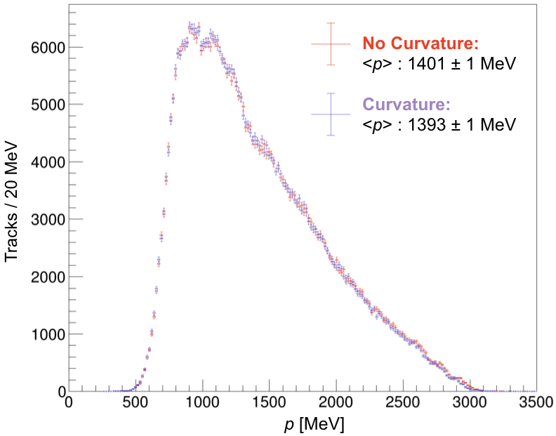
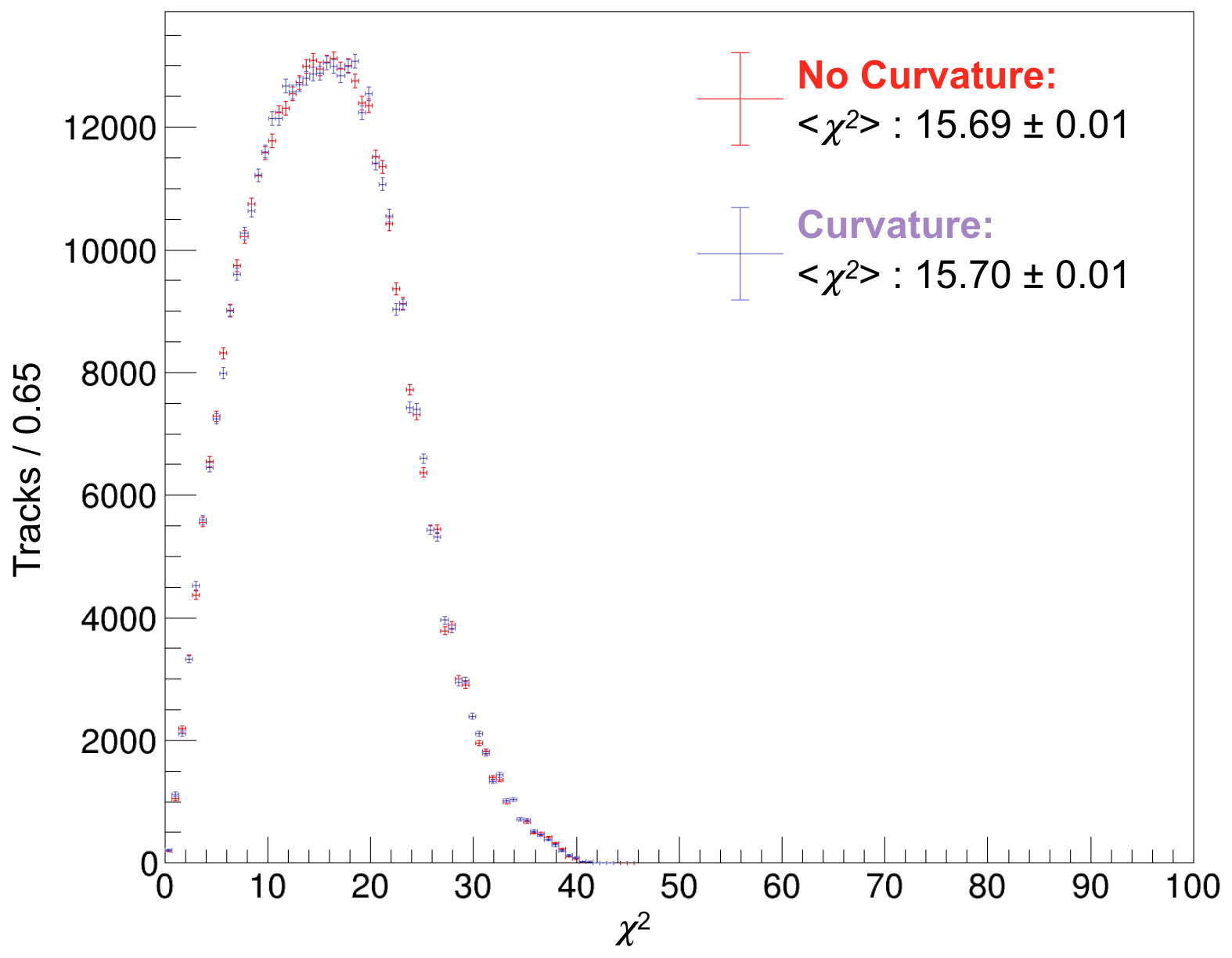
Moreover, if a module is misaligned internally, this is manifested as a deviation from the overall radial detector curvature in that module, as shown in Figure 8.4.
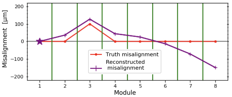
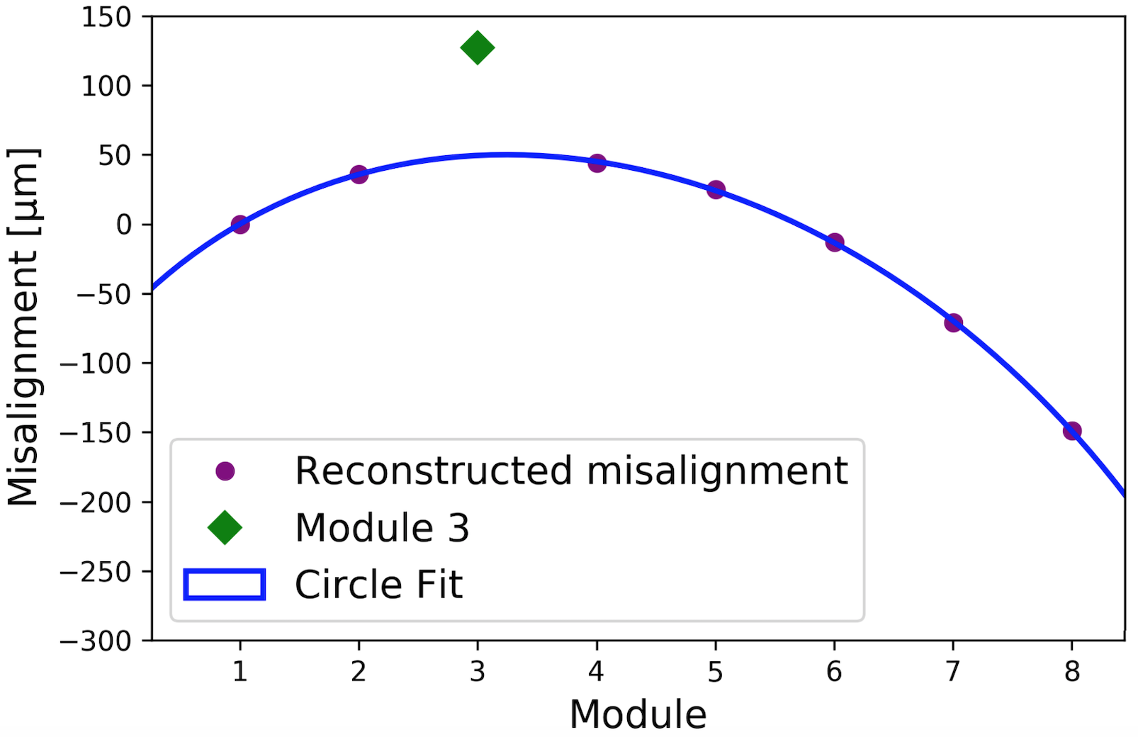
However, if the correct constraints from Equation C.4 are used, the radial detector curvature effect is removed completely as shown in Figure 8.5.
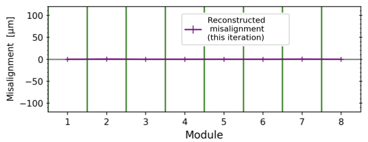
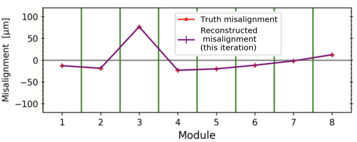
8.3 Methodology
This potential radial detector curvature, (see Equation 7.30), needs to be measured independently of the internal alignment, analogous to the global alignment measurements, described in Appendix A. One property that makes this measurement possible is the momentum-dependence, , of the extrapolated tracks with respect to the input detector curvature, as shown in Figure 8.6.
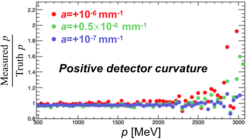
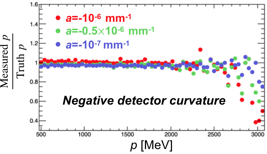
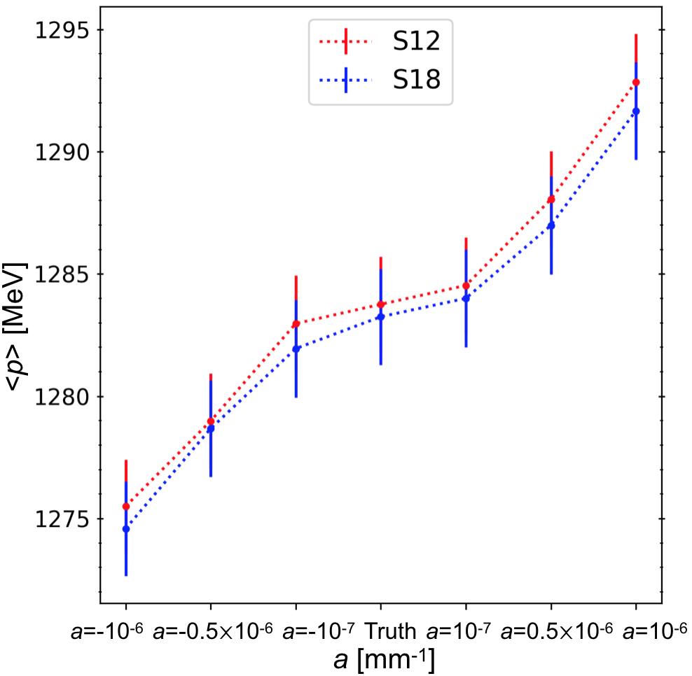
A standalone toy-model for this momentum-dependence of the curvature as a function of momentum is shown in Figure 8.7.
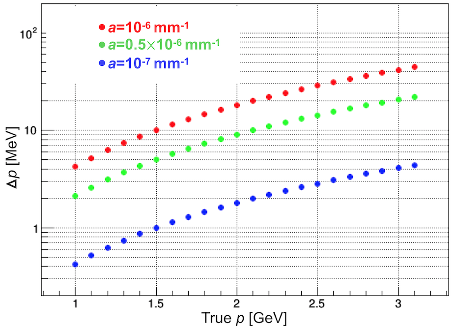
The previously seen effect is confirmed: larger curvatures have a larger impact on the track momentum, and high momentum tracks have the largest response to a given curvature. To further study this effect, laser-survey data (see Appendix A) of the modules was used to define a reasonable curvature range of the modules.
The laser-survey alignment has an error of on an individual module position. This error can be used to fit a nominal (best fit) curve to the module positions. The curvature parameter () is extracted directly from a fit to Equation 7.30, along with the curvature parameters that lie within a 1 band of the nominal curvature. These are obtained using the Mahalanobis method [86]. For a three parameter fit, there are 27 possible Mahalanobis fits. These fits are shown in Figure 8.8, and the parameter for these fits are shown in Figure 8.9.
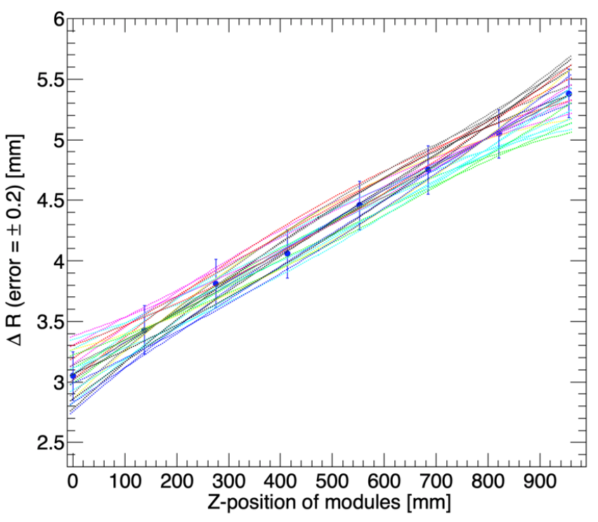
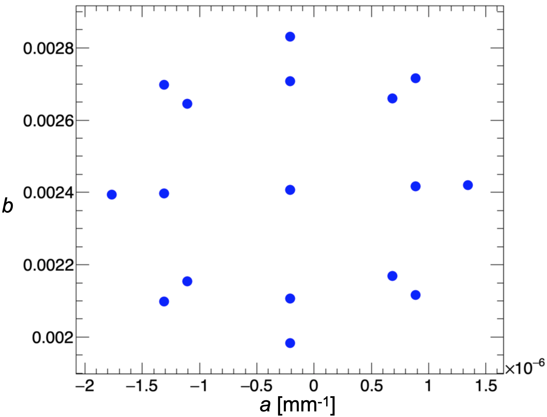
8.3.1 Data-simulation comparison
Equation 7.30 and the estimated curvature parameters from Figure 8.9 were used to misalign tracker modules in a curved position in the simulation. A comparison of the various curvatures with data, where this additional curvature was not applied, was then performed. The assumption is that the simulated curvature that best matched the data is the corresponding curvature in data. The comparison criteria was the extrapolated radial beam position, as shown in Figure 8.10, for a selection of the most closely matched curvatures in station 18. The extrapolation on data was performed after internal and external alignments as described in Section 7.5 and Appendix A, respectively. Moreover, the simulation’s beam distribution was tuned to match the data in Run-1 (see Section 3.4.4).
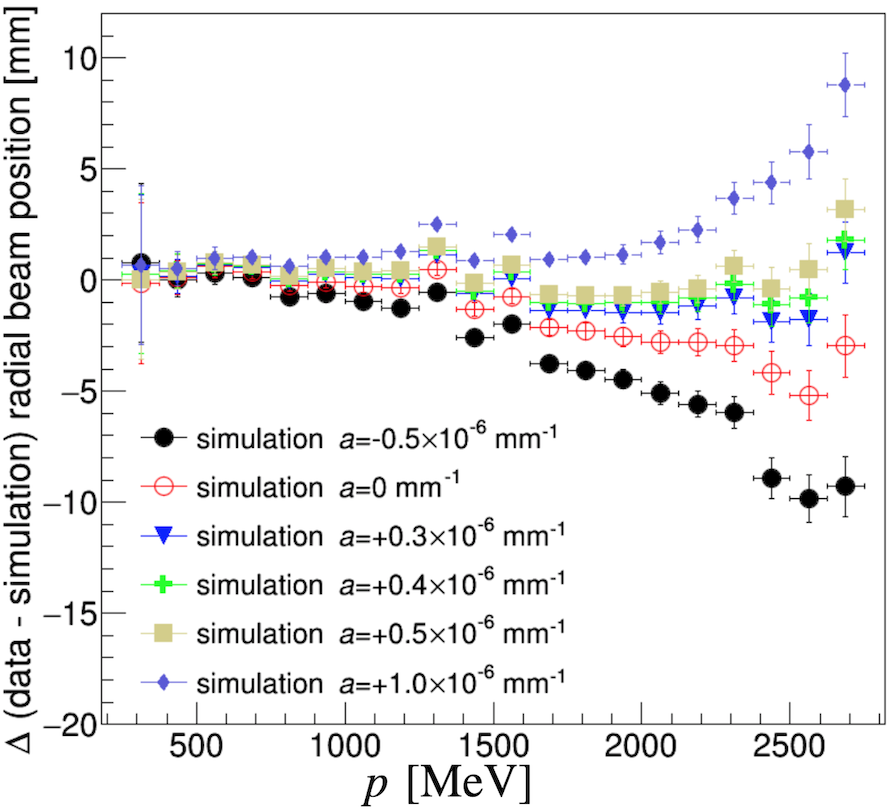
8.3.2 Comparison methods
The results in Figure 8.10 can now be compared using the method. This is done by calculating the per momentum bin for a given simulation curvature
| (8.1) |
as the function of , the amount of radial shift (for all momentum bins) needed in simulation to align the extrapolated curve with data, such that
| (8.2) |
The assumption is that the simulation result with the smallest corresponding is the best representation of the curvature in the data. An example scan over for a curvature of is shown in Figure 8.11.
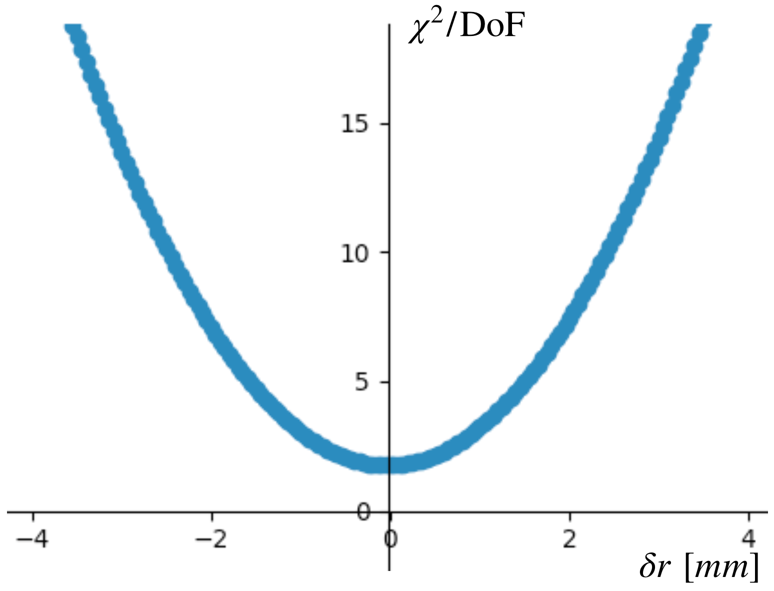
The final results of the method are summarised in Figure 8.12a. Alternatively, as a cross-check, a residual method can be used. This method calculates for each momentum bin, and extracts the lowest absolute value of over many curvatures from
| (8.3) |
The results from the residual method are summarised in Figure 8.12b.
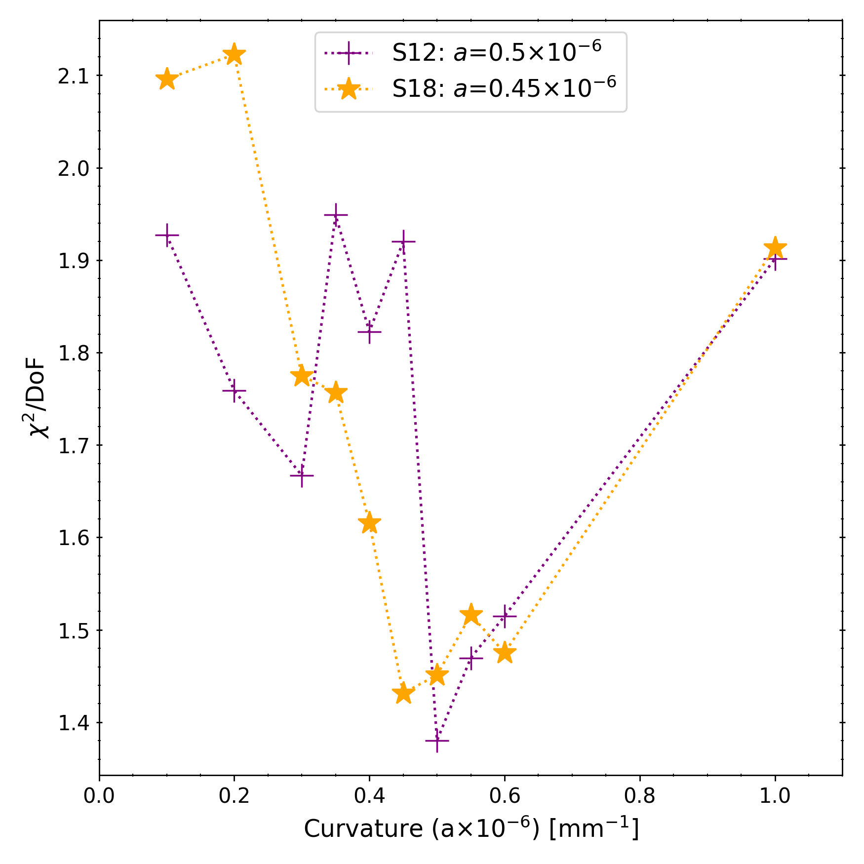
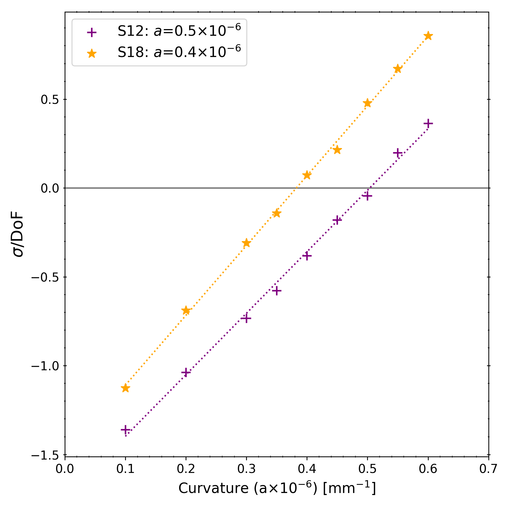
8.3.3 Extrapolation with detector curvatures
To examine the effect of these curvatures, tracks were re-fitted with a curvature offset and the tracks were extrapolated back to determine a beam position. This shift of this beam position, both radially and vertically, from the nominal, is shown in Figure 8.13.

Finally, a similar scale of curvatures can be applied to data, as shown in Figure 8.14. The uncertainty coming from the detector curvature estimated by comparison with simulation can now be directly extracted from these plots.
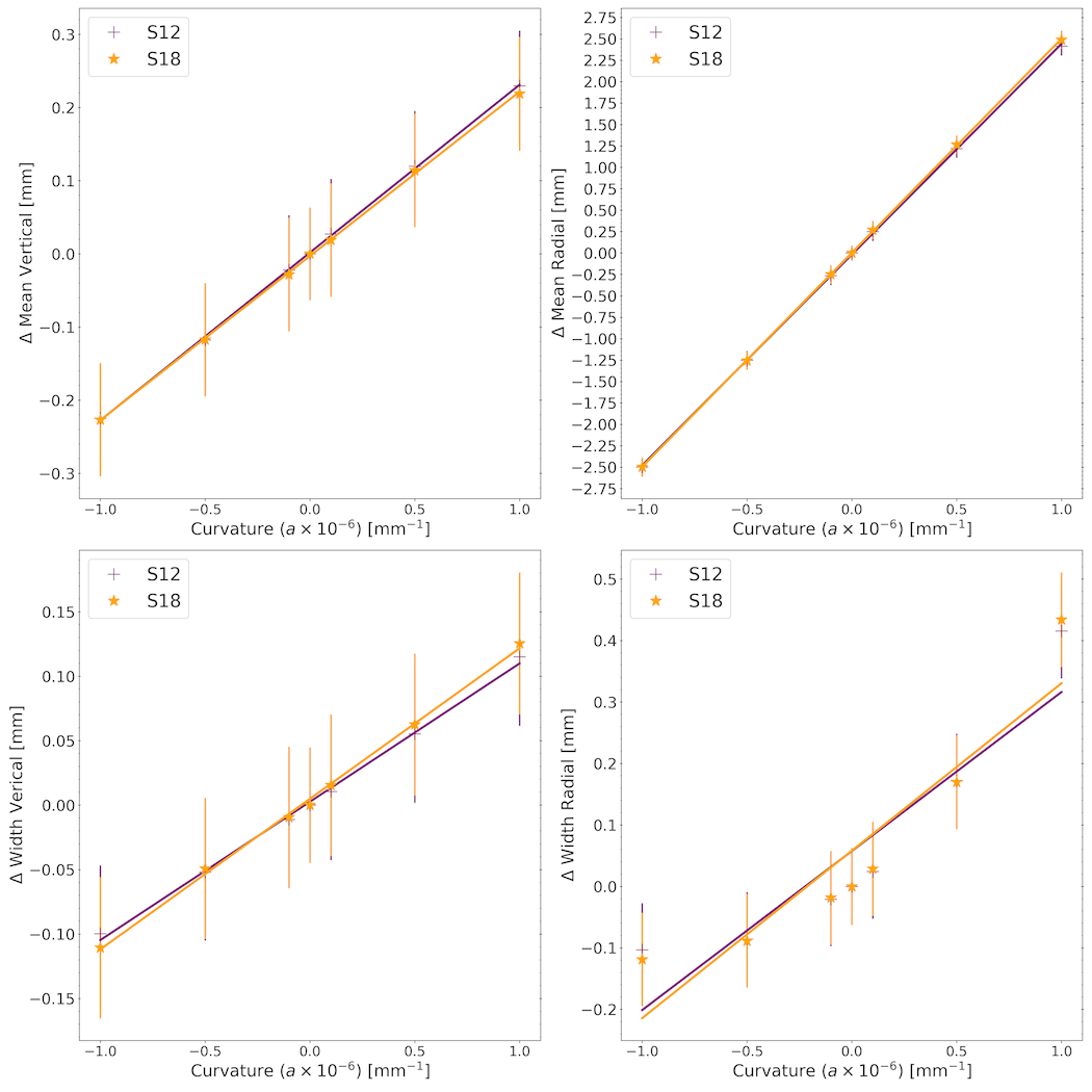
8.4 Results and outlook
The beam extrapolation determines the radial and vertical positions of the muon beam in the storage ring. The accuracy of this determination is affected by detector effects, such as the radial detector curvature. To estimate the contribution of the detector curvature to beam extrapolation, the largest of the values from the two methods in Section 8.3.2 was used, for a conservative estimate. This value is , and the corresponding beam extrapolation uncertainties, extracted from Figure 8.14, are given in Table 8.1.
| [] | [] | [] | [] | |
|---|---|---|---|---|
| S12 S18 | 1.25 | 0.20 | 0.10 | 0.05 |
However, there is a motivation to improve the detector curvature estimation, given it is one of the larger tracking systematics (see Section 3.4.1). Some of the possible improvements are given below:
-
•
Improved tracking and simulation. An improvement to the tracking algorithms will allow for a more precise limit on the curvature to be placed. Such improvements include LR assignment, hit selection, and improving track quality, and are being developed by G. Sweetmore [87], S. Grant [88], and A. Luca [85], respectively. Moreover, an improved simulation, that is more representative of real data will also benefit the curvature study.
-
•
Cosmic muons. An alternative estimation of the curvature is possible with cosmic ray muons during periods when the magnetic field in the ring if off. However, there are numerous challenges associated with this study, such as maintaining long periods without the magnet on, developing a precise straight-track fitting algorithm, and estimating the residual magnetic field.
8.5 Impact on the systematic uncertainties
8.5.0.1 Pitch correction ()
Using Equation 3.11, and an upper bound on from Section 8.3.2, with the corresponding mm (see Table 8.1), yields ppb.
8.5.0.2 Field convolution ()
A study of an impact of translations on the extrapolated beam profile from the tracking detectors on the field measurements was performed by Jason Bono and Saskia Charity [71]. Given the scale of translations induced by the curvature of , of 1.25 mm and 0.1 mm radially and vertically, respectively (see Table 8.1). It is possible to estimate the corresponding uncertainties on , and hence (see Equation 3.2). The results for both stations are given in Table 8.2, with the average vertical and radial uncertainties in both stations on of 12.9 ppb and 0.6 ppb, respectively.
| S12 radial | S18 radial | S12 vertical | S18 vertical |
| 11.6 ppb | 14.2 ppb | 0.6 ppb | 0.6 ppb |
Chapter 9 A preliminary track-based analysis
This chapter presents preliminary results from the first attempt at an analysis with data from the tracking detector. This type of analysis has the advantage of having a different set of systematic uncertainties (e.g. pile-up, \saylost-muons), as compared to the calorimeter-based analysis. The available statistics in the tracker-based analysis is significantly lower. However, given the previous measurement’s discrepancy with the theory of ppm (see Section 2.1) and if the tracking detector measures the same value as the BNL, then to exclude the theoretical prediction at CL requires a measurement with a precision of ppm. In this chapter, an estimate is made of when this threshold will be reached with the acquisition of more data, based on the preliminary analysis of Run-1 data.
9.1 Analysis overview
The analysis work in this chapter follows closely the methodology of the analysis using calorimeter data [41, 57, 66]. The first statistical assessment of Run-1 data, applying time cuts (see Section 3.3.3) and momentum cuts (see Section D.2), is summarised in Table 9.1. The number of tracks (above the threshold) is times less than the number of (above the threshold) recorded by the calorimeters (c.f. Table 3.1 with Table 9.1).
| Dataset | All quality | Quality tracks | Quality tracks |
|---|---|---|---|
| name | tracks | () | (, GeV) |
| 1a | |||
| 1b | |||
| 1c | |||
| 1d | |||
| Total |
9.1.1 Five-parameter fit
The first step in the analysis was a simple five-parameter fit to the number of quality tracks as a function of time
| (9.1) |
where is the overall normalisation, is the time-dilated muon lifetime, is the asymmetry, and is the phase. The value of returned from the fit is blinded in software and hardware (see Section 4.1.2), so that a value of (see Equation 4.2) is reported instead. The result of the fitting procedure is shown in Figure 9.1. Such a plot is known colloquially as a \saywiggle plot. The choice of the width of a bin in this histogram is ns, the cyclotron period. It is important to note that the start-time of the fit should be at the edge of a bin; otherwise, the fit quality is negatively affected.
The quality of the above fit can be assessed in terms of the distribution of the fit pulls (i.e. normalised residual between the fit function in a given time bin and the data), as shown in Figure 9.2a.
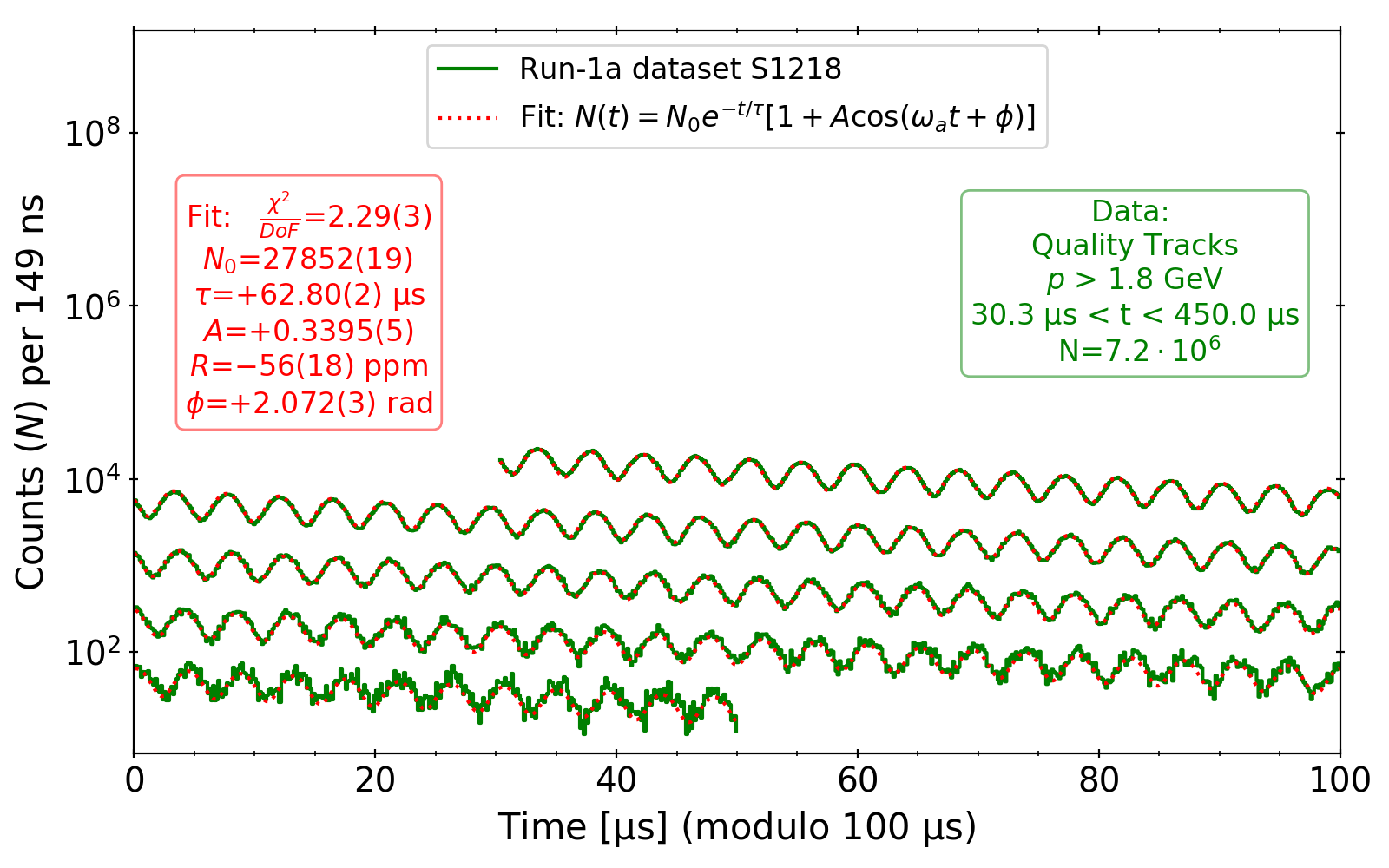
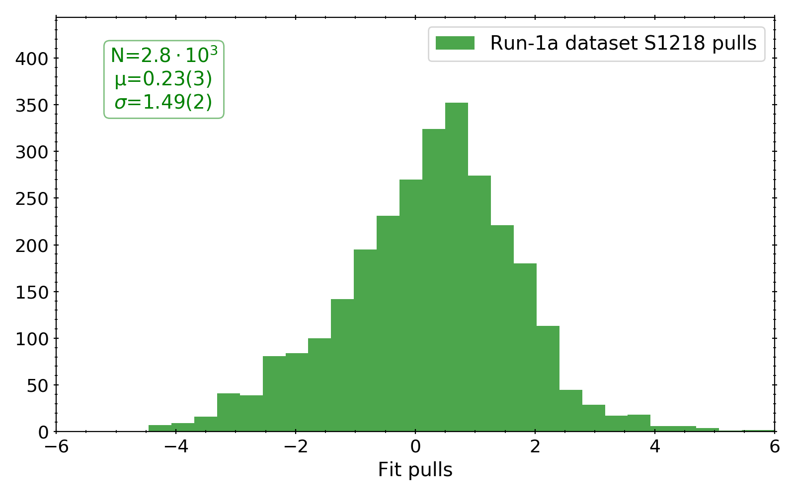
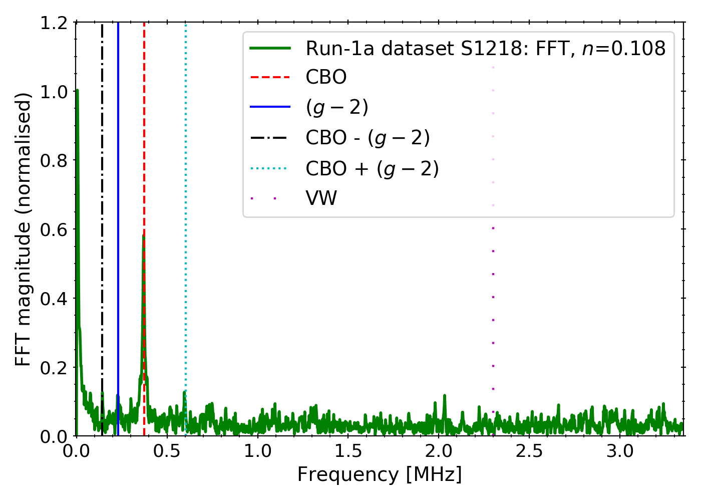
The non-centred distribution of fit pulls with significantly larger than suggests that the chosen function doesn’t describe the data well. This can be further verified by transforming the residuals from the time to the frequency domain, using a fast Fourier transform (FFT) [89]. A large peak at MHz is observed, which is likely due to effects from lost-muons or pile-up. Moreover, a peak at the CBO frequency (see Section 3.4.2) is also seen, which also couples to the frequency, ,
| (9.2) |
The expected frequencies of the peaks in Figure 9.2b depend on the field-index, (see Section 3.3.3 and Table 3.1.).
9.1.2 Nine-parameter fit
The presence of the large FFT peak at the CBO frequency motivates incorporating additional terms in the fit function, which describe the impact of the CBO on the number oscillation, such that
| (9.3) |
where is the CBO function [90] given by
| (9.4) |
Equation 9.4 is analogous to the original five-parameter function, but with each term now describing the CBO parameters: lifetime (), amplitude (), angular frequency (), and phase (). This fit is shown in Figure 9.3a. With the CBO terms in the fit, the is improved. To verify that the correct model was used to describe the CBO’s influence on the oscillation, the FFT analysis was repeated as shown in Figure 9.3b. The CBO peak is no longer present.
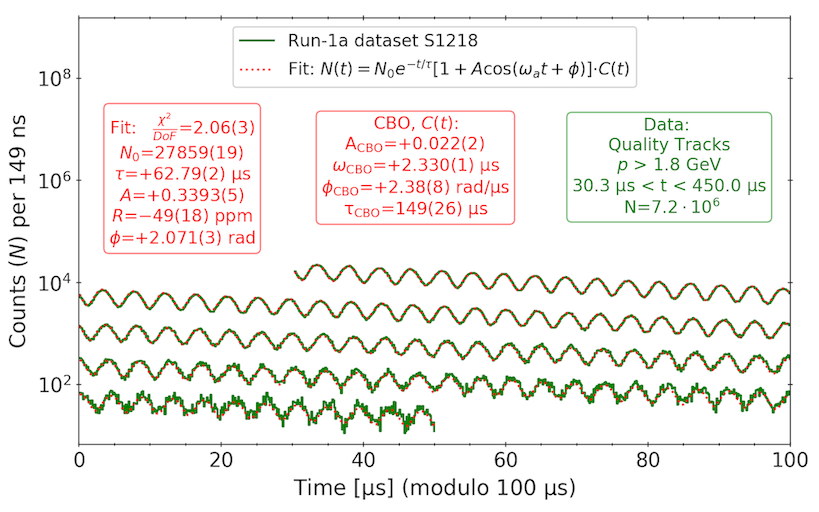
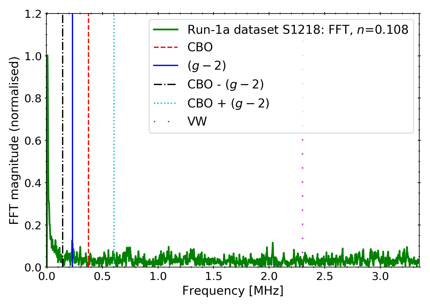
9.1.3 Ten-parameter fit
The remaining feature in the FFT spectrum in Figure 9.3b that needs to be accounted for is the peak at MHz. The physical origin of this feature are lost-muons (see Section 3.4.6). This can be incorporated by adding a term accounting for the lost-muons in the fit, such that the fit equation becomes
| (9.5) |
where is
| (9.6) |
the lost-muon term, with an arbitrary fit parameter (i.e. normalisation). In this analysis, was taken from [66]. It should be noted, however, that [66] defines the rate of lost-muons for a calorimeter-based determination of . The different acceptance of the tracking detectors means it is at best an approximation of the lost-muon rate for a track-based analysis. Nevertheless, incorporating the lost-muon term yielded improved results, as compared to the nine-parameter fit, as shown in Figure 9.4. The fit can be further improved by adding systematic effects to the fit (e.g. pile-up), or performing a dedicated lost-muon analysis in the tracking detector. However, the fit quality is sufficient for this preliminary analysis to be able to estimate the statistical precision on the tracker-based determination of .
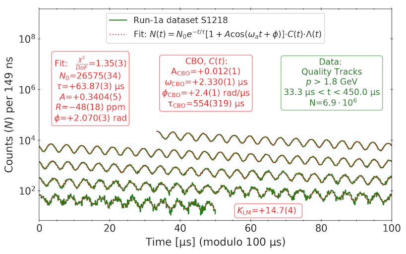
With the ten-parameter fit, the slow effect is now diminished as seen in the improved distribution of fit pulls in Figure 9.5a, and the prominent peak at MHz is significantly reduced, as seen in Figure 9.5b.
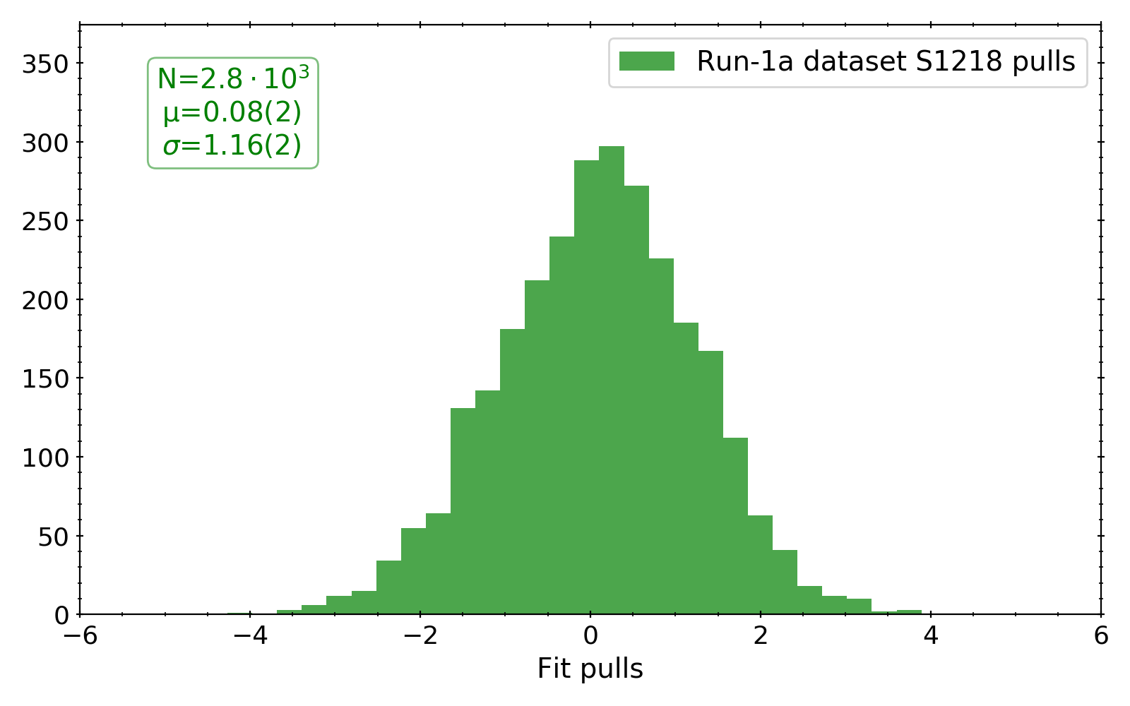
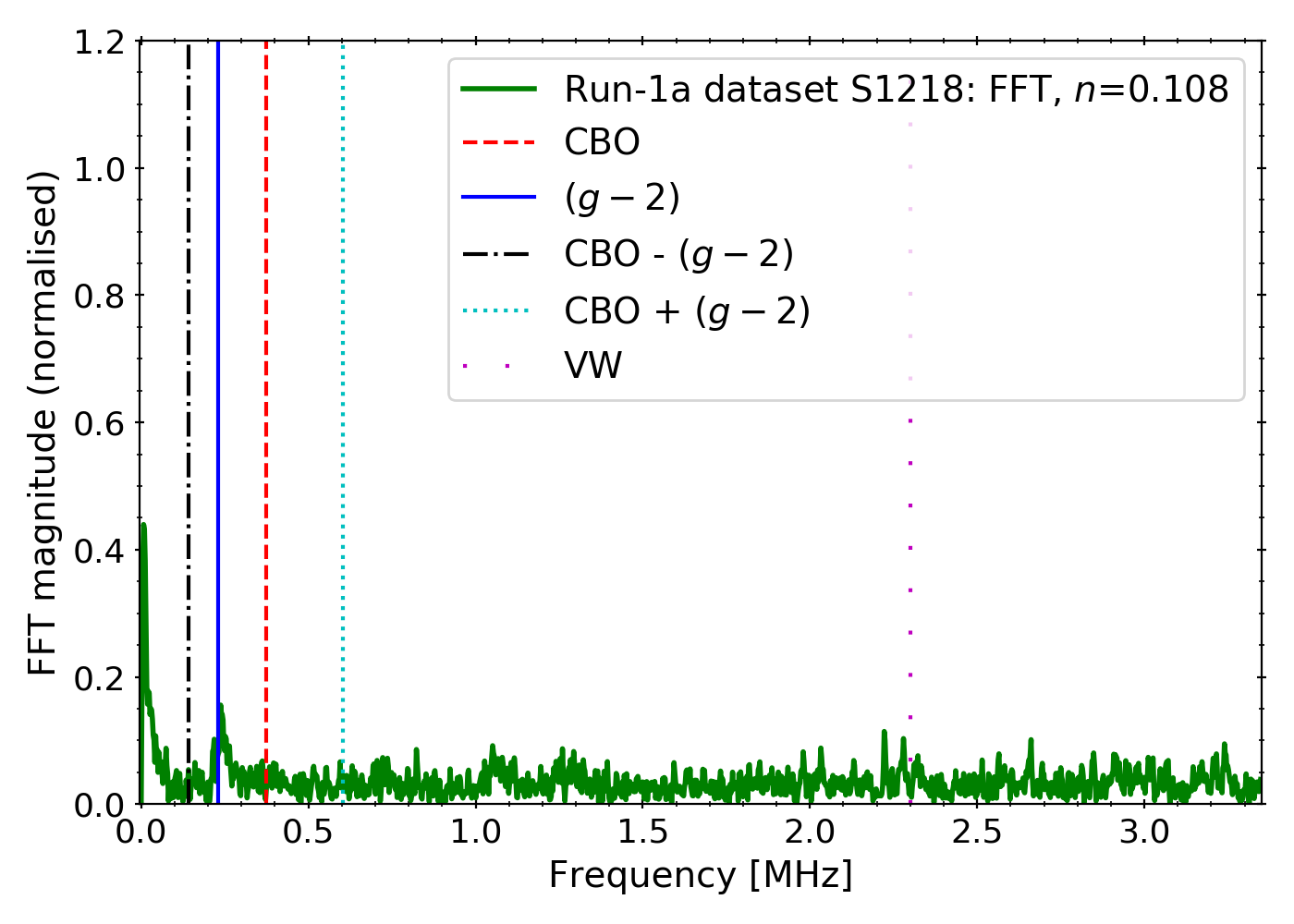
9.2 Results
The statistical uncertainties on , obtained from a ten-parameter fit, for all four Run-1 datasets are summarised in Table 9.2, while the corresponding plots are contained in Section D.1.
| Dataset | 1a | 1b | 1c | 1d |
|---|---|---|---|---|
| (ppm) |
The combined statistical uncertainty can be approximated [91] via
| (9.7) |
which assumes a Gaussian distribution of errors and no correlations between the datasets. To verify this estimation, the statistical uncertainty on of 1.4 ppm from a fit of calorimeter events [66] in the Run-1a dataset can be used to predict the expected precision on the tracker data of events, yielding
| (9.8) |
The estimated uncertainties in Equations 9.7 and 9.8 compare well, given the precision on the calorimeter data is derived from a fit with better estimates of systematic effects.
It is now possible to calculate the number of tracks required to reach a defined precision on , and hence , given that tracks yield a ppm uncertainty. Therefore, to reach a precision on the measurement of 1.4 ppm, and thus confirm the BNL-SM discrepancy at CL, should the same value be measured, would require tracks. While to reach a comparable precision of the final measurement at the BNL, of 0.54 ppm [1], would require the experiment to accumulate tracks.
9.3 Outlook
For the tracker-based determination of to become competitive, more tracker data must be acquired, and the tracking efficiency increased. This efficiency is described in Section 5.3.8, and will be applied to the already-collected data, yielding at least a factor of four increase in the number of tracks.
Using Figure 3.17a, a relation can be made between the raw number of collected in Run-1 and the number of tracks that were used in this preliminary analysis. A projection can than be made, using Figure 3.18a, on the expected number of tracks that can be used in the determination of . This projection, shown in Figure 9.6, is based on the assumption that the increase in the quality data (see Section 3.8.1) will be between and [92, 93], as compared to Run-1. Given the current improvements in tracking, a CL limit can be placed by Run-3. With further improvements, a comparable precision to the one achieved at the BNL (with calorimeter data) can be reached by Run-5 with the Fermilab tracking detectors alone.
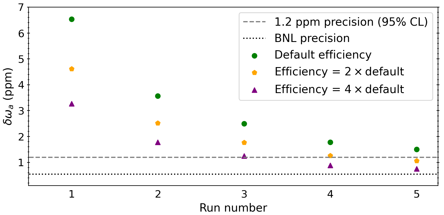
Chapter 10 Systematic studies of the EDM
This chapter describes the methodology of the EDM measurement using data from the tracking detectors. Section 10.2 contains the results of the EDM analysis in the simulation. The impact of radial and longitudinal magnetic fields on the EDM and determination is introduced in Section 10.3, while the results of their measurements are given in Section 10.4 and Section 10.5, respectively.
10.1 Introduction
The effect of a potential EDM of the muon, which was introduced in Section 2.2, would result in a tilt of the muon spin precession-plane as shown in Figure 10.1. This tilt changes the observed precession frequency by an addition of the precession resulting from a muon EDM [6], ,
| (10.1) |
Equation 10.1 describes the muon experiencing a torque in the presence of the electric field produced by the ESQs, as well as the apparent electric field in the muon rest-frame resulting from the Lorentz boost to the laboratory-frame magnetic field [15]. is orthogonal to the vertically oriented , and is pointing radially inwards towards the centre of the storage ring. This results in the spin precession-plane tilting out from the orbit plane towards the centre of the storage ring.
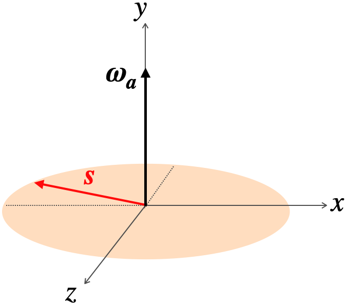
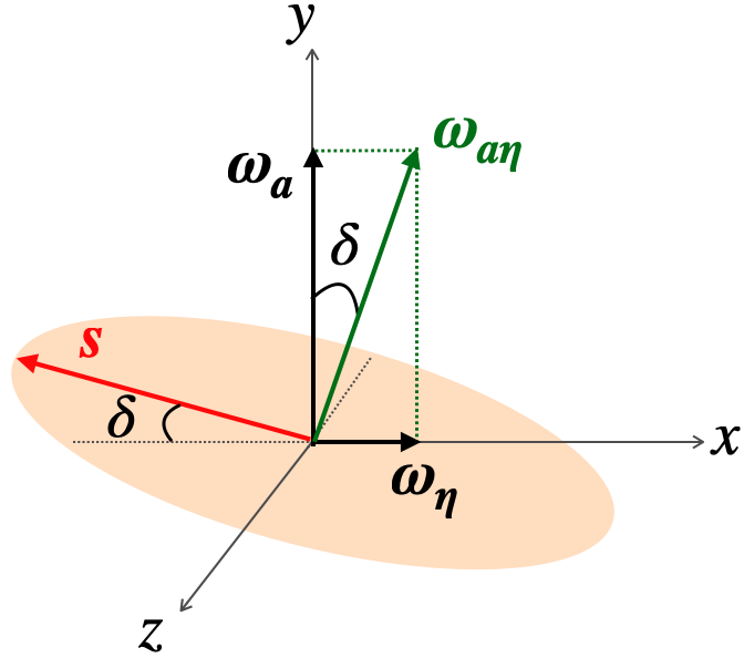
There are two important consequences of a non-zero muon EDM: an increase in the observed precession frequency, and an introduction of an oscillation of the average vertical angle of the emitted positrons from the muon decay. The magnitude of the observed precession frequency is now given by
| (10.2) |
The resultant tilt angle of the spin precession-plane in the muon rest-frame, , is given by
| (10.3) |
As the positrons are preferentially emitted along the direction of muon spin (see Figure 2.3), the tilt will make the positrons on average downward going when the spin is pointing towards the centre of the storage ring, and upward going when the spin points away from the centre of the ring. Therefore, the observed average vertical angle varies with the magnitude of , and this angle is the observable that is used in the experiment to measure the EDM using the tracking detectors.
Finally, it is essential to emphasise that when the muon spin and momentum vectors are aligned, the maximum signal is observed. However, the vertical angle oscillation is at the maximum when the spin is pointing radially outwards, that is, out-of-phase with the momentum vector. This property is used to distinguish between an EDM and other effects, which are in-phase with , that can also impact the vertical angle oscillation. This is discussed in Section 10.3, for potential non-zero radial and longitudinal magnetic field components.
10.2 EDM search with the tracking detectors
The goal of the Fermilab experiment is to measure to within , resulting in a sensitivity to an EDM of cm [14]. The tracking detectors will realise an EDM measurement through the direct detection of an oscillation in the average vertical angle of the decay positrons. The tracking detectors measure this vertical angle, , through the momentum components of a track
| (10.4) |
For example, a distribution of measured vertical angles in the Run-1a dataset are shown in Figure 10.2, with a width of mrad.
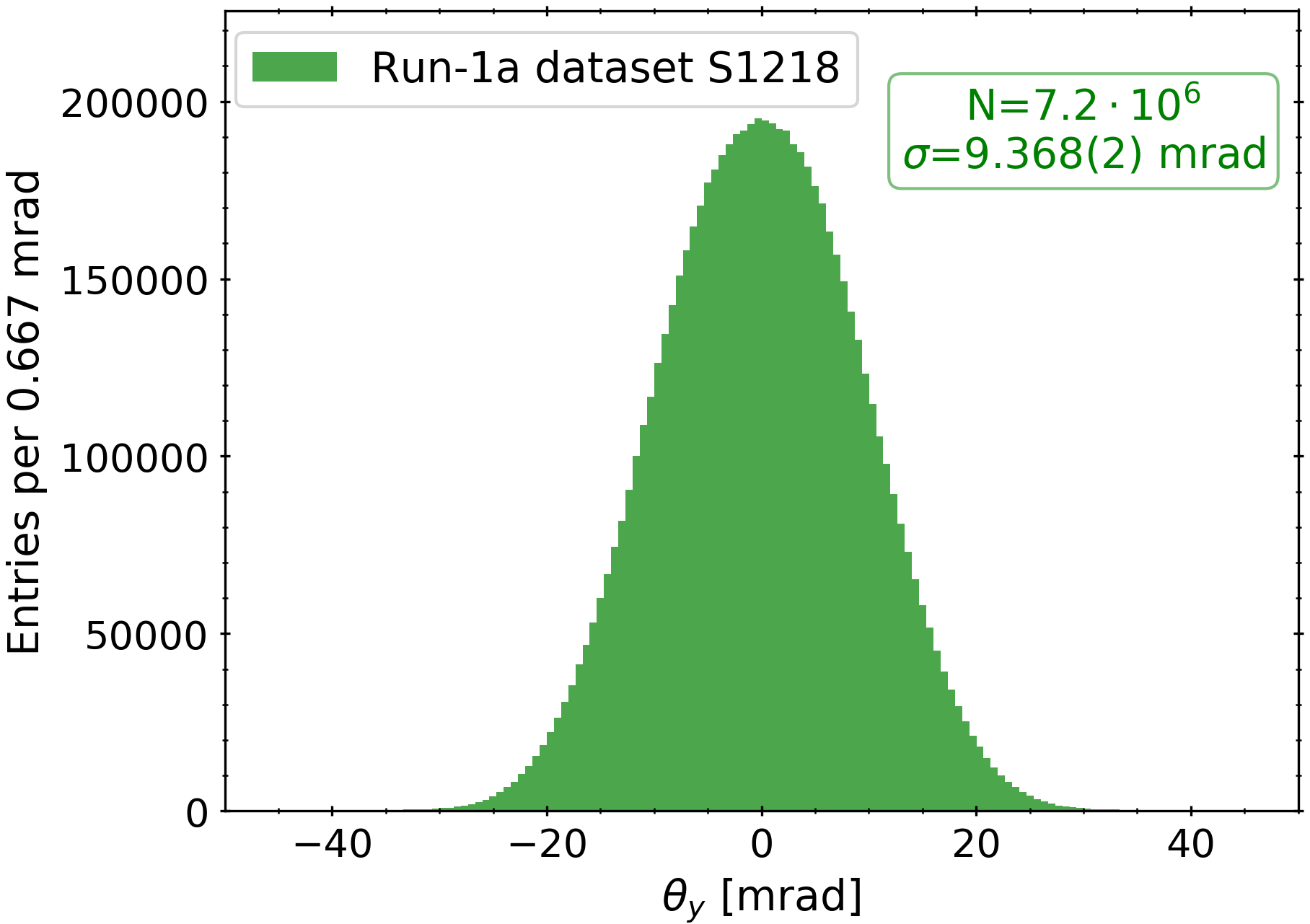
10.2.1 Simulating a large EDM signal
In order to test and develop the analysis techniques, a simulation with a known value of the EDM was used. The chosen value of the EDM was , which corresponds to a value times larger than the EDM limit set at the BNL experiment [15]. This value was chosen to resolve the EDM signal with a relatively low number of available tracks from simulation and permitted a cross-check with previous simulation results [68].
It is possible to analytically predict the observed oscillation amplitude, , of
| (10.5) |
where is the precession-plane tilt angle in the lab-frame, and is the asymmetry of [94], which accounts for the fact that not all positrons are emitted in the direction of the polarisation vector. The tilt angle in the muon rest-frame, , is accessible via a Lorentz boost (see Section D.3)
| (10.6) |
Finally, substituting from Equation 2.7 into Equation 10.3 allows to be directly expressed in terms of fundamental constants and the input EDM signal ()
| (10.7) |
10.2.2 EDM measurement strategy in the simulation
To observe the oscillation of the vertical angle, and hence measure , it is necessary to consider how changes with time, as shown Figure 10.3a, where is the track time in a fill. This time is then modulated by the period ( ), ,
| (10.8) |
This is analogous to the method used in the BNL EDM analysis [95], which is known as the period-binned analysis. This modulation method is useful for looking at periodic effects, such as the vertical angle oscillation. Periodic effects that do not have the same period as (e.g. betatron oscillations mentioned in Section 3.4.2) will generate a flat background when many periods are considered, while the signal of interest adds constructively. The time modulation, , is given by
| (10.9) |
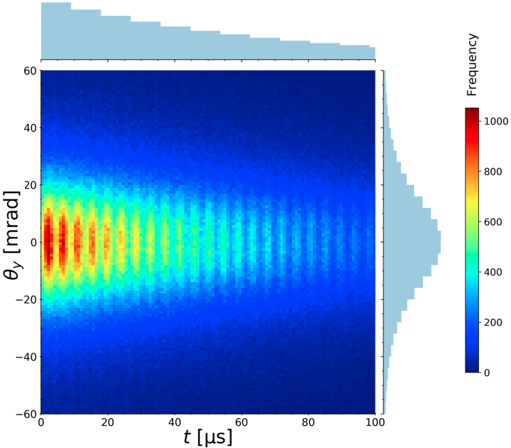

was then profiled (i.e. averaged) into ns bins, as shown in Figure 10.4. The distribution of in each time bin is Gaussian, as shown in Figure 10.2. The observed oscillation of the averaged vertical angle, , is given by
| (10.10) |
where is the overall offset in . Equation 10.10 is the fit function used in Figure 10.4. The fitting is done using the scipy.optimize Python library. The optimal momentum and time cuts for this analysis are discussed in Section 10.5.4. The extracted value of is mrad, which agrees well with the prediction from Equation 10.7.
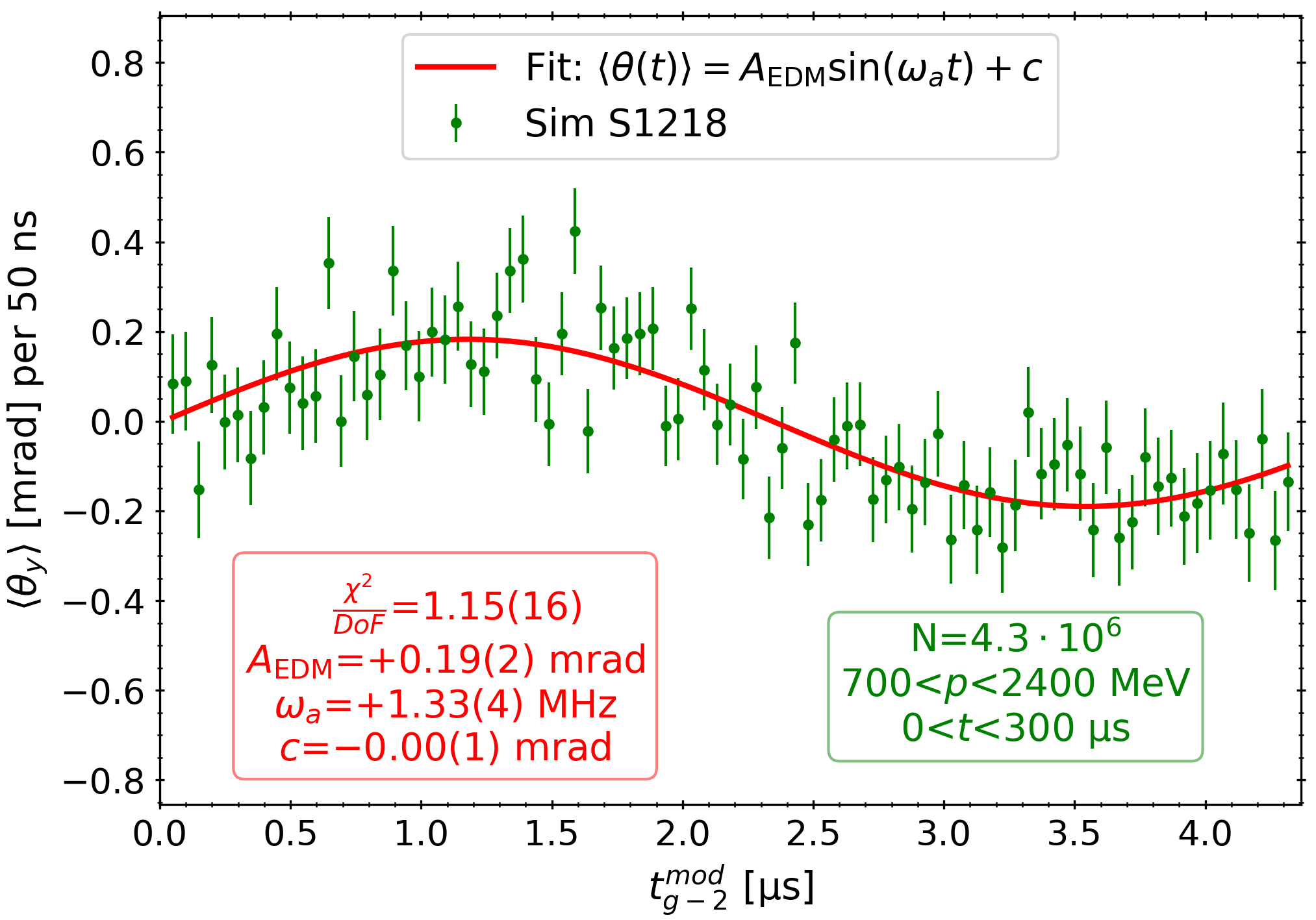
10.3 The significance of non-zero magnetic fields
The experiment is designed to have only the vertical component of the magnetic field, with both radial and longitudinal components being zero. In the experiment, the vertical magnetic field, , is measured directly by the NMR probes to an accuracy of 70 ppb, as described in Section 3.5. However, no such direct measurements presently are possible to determine the radial, , or longitudinal, , fields. Non-zero or can tilt the precession-plane of the muon, as shown in Figure 10.5. This becomes an important systematic effect for both the EDM and analyses, as can be seen by adding two aforementioned magnetic field terms to Equation 3.1
| (10.11) |
It is important to note, that would have the same effect on the precession-plane as the EDM (c.f. Figure 10.1). It is, therefore, crucial to estimate in order to not bias the results of a search for the muon EDM. Various strategies exist to estimate , both direct [96] and indirect. The approach taken in this thesis is the indirect measurement of using the tracking detectors, as described in Section 10.4.
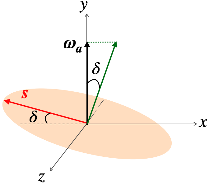
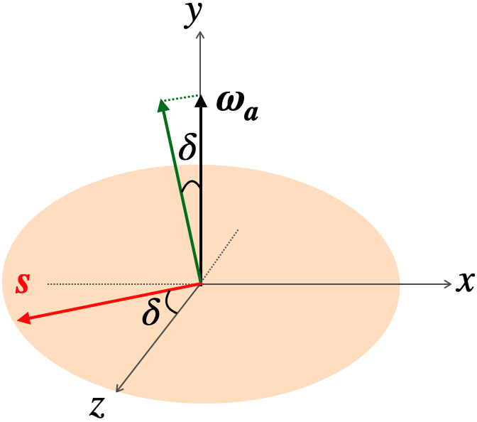
A non-zero , on the other hand, would tilt the precession-plane in the direction of the muon momentum vector. This produces an effect that manifests as an EDM-like signal that is in-phase with the magnetic dipole moment (i.e. in-phase with ) and out-of-phase with the EDM (see Section 10.1). Therefore, one way to measure is to perform a search for the in-phase signal using data from the tracking detectors, as described in Section 10.5.
10.4 Preliminary estimation of
10.4.1 Introduction
In the BNL experiment, the EDM limit is \sayequivalent to a 30 ppm , while the determination of was estimated with a precision of 10 ppm [15]. Had the experiment had enough statistics, they would have been limited at due to the uncertainty on , as demonstrated in Figure 10.6. Therefore, in the Fermilab experiment more precise measurements of , both direct and indirect, are motivated to allow for an improved measurement of the EDM. An accuracy of 0.2 ppm is required to probe at the cm level.
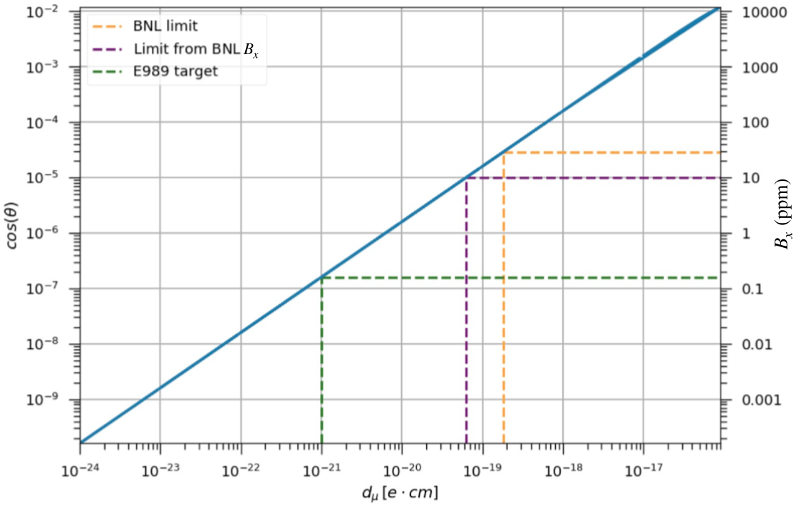
The aim of this preliminary study was to estimate by varying the electric field produced by the ESQs (see Section 3.3.3) and measuring the resultant mean vertical beam position, , using the tracking detectors, and using the relation [98]
| (10.12) |
where is the field-index (see Section 3.3.3), is the storage ring radius, and is the magnetic field strength. contains the electric field gradient of the ESQs, which is directly proportional to the HV applied to the ESQs – QHV. Increasing the value of QHV should result in the observed value of decreasing, and vice versa. Equations 10.12 and 3.6 allow the estimation [99] of
| (10.13) |
where is the variable, and is the observable, and can be determined from tracker data. The objective is to verify the viability of such a measurement.
10.4.2 Results
There were two periods in Run-2 that had a change in QHV: 20 June 2019 and 24 March 2019.
The QHV settings versus time for 20 June are shown in Figure 10.7. To ensure the measurement of is only influenced by the QHV, settings of other components (e.g. kicker voltages) are required to be constant. The difference in the measured values of , at a given QHV setting, between the two tracker stations, as seen in Figure 10.7b, are expected and their origin discussed in Section 3.4.5.
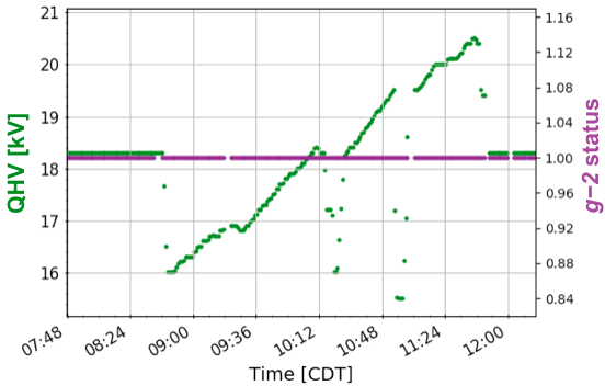
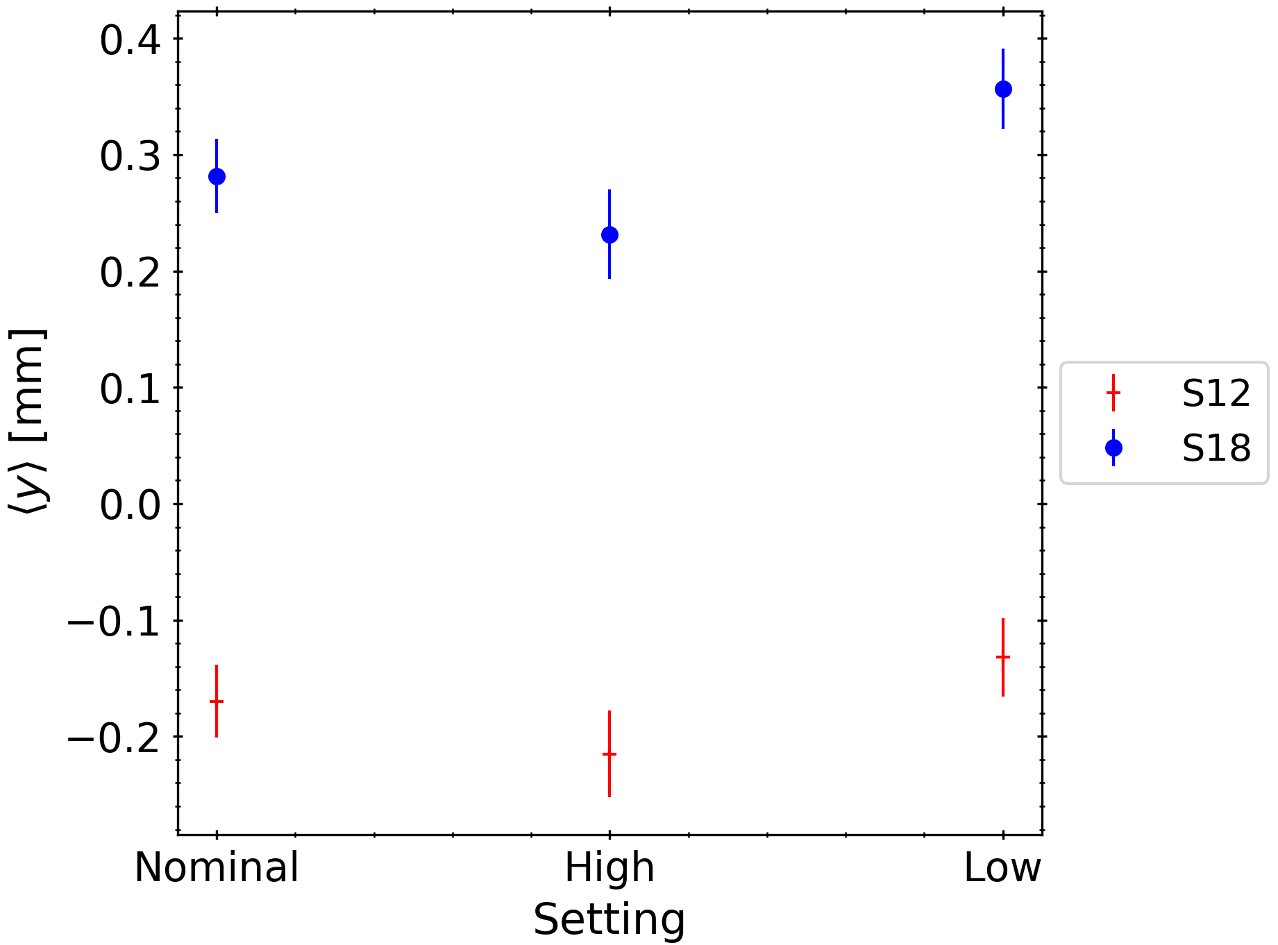
in tracker station 12 (20 June) is plotted against (QHV)-1 in Figure 10.8a. Using the obtained slope from Figure 10.8a and Equation 10.13, an estimation of is possible. The final result, ppm, is summarised in Figure 10.8b.
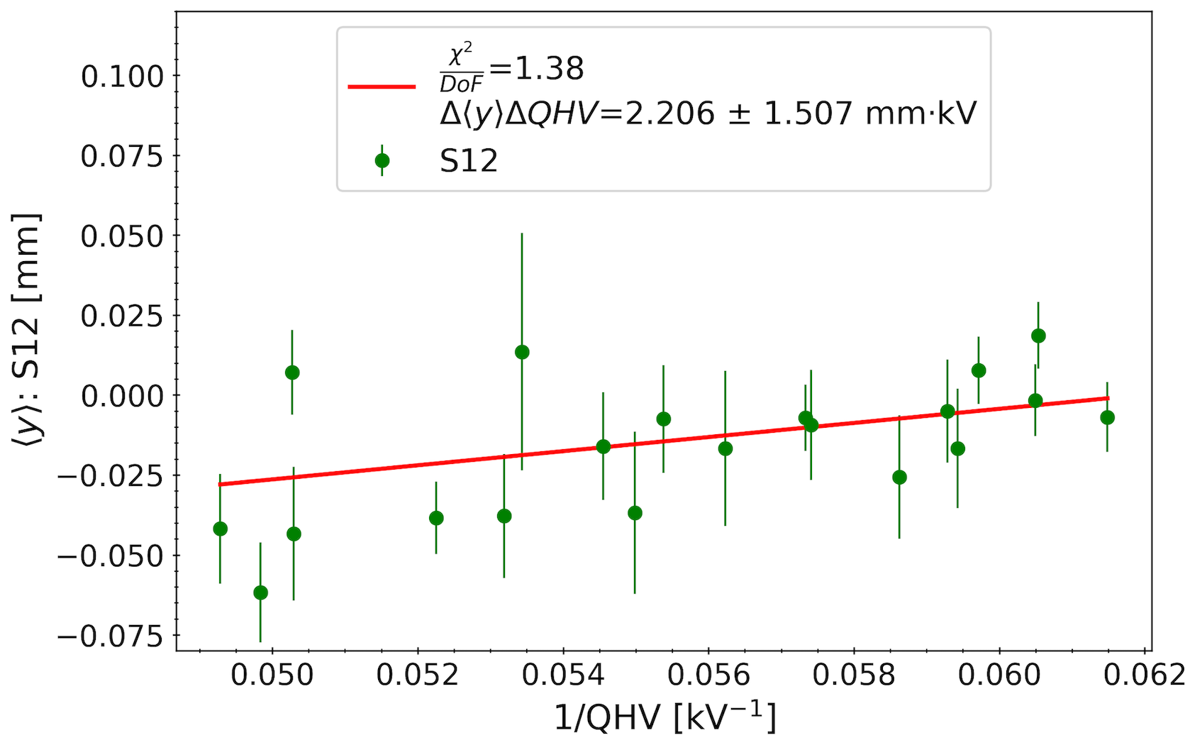
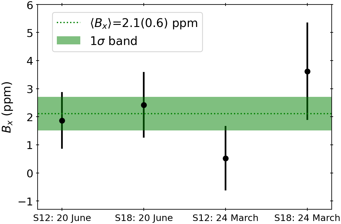
10.4.3 Outlook
In this study, the preliminary-estimated value of in Run-2 of ppm falls short of the required precision of 0.2 ppm, as outlined in Section 10.4.1. Therefore, more precise measurements of , both direct and indirect, are motivated to allow for a more precise determination of the EDM. An improved method to determine was suggested by B. Kiburg [100]. This method will determine by a variation of QHV together with an applied radial field gradient, , from the correction coils (see Section 3.5), that will induce a large, and known,
| (10.14) |
where is the unknown variable in this equation. A direct measurement of is also being developed by M. Fertl [101].
10.5 Estimation of
The presence of a longitudinal magnetic field, , tilts the precession-plane of the muon, as shown in Figure 10.5. It is therefore imperative to accurately and precisely measure . As discussed in Section 10.3, a non-zero introduces an up-down oscillation of the vertical track angle, in-phase with . This oscillation is used in this analysis to determine . This analysis follows a similar methodology as the EDM simulation study described in Section 10.2.2. Following the method used in the BNL experiment [95], two fits are performed. Firstly, the number of quality tracks is time-modulated according to Equation 10.9, and is determined using the five-parameter fit of Equation 9.1 but with fixed at the value measured by the BNL experiment, [1]. The average vertical angle oscillation, , is then fitted to the function
| (10.15) |
where is the amplitude due to the longitudinal magnetic field, is the EDM amplitude, and is an overall offset.
10.5.1 EDM blinding
As seen from Equation 10.15, the EDM amplitude is directly accessible. This is not desirable when analysing data, as the aim is to measure without revealing . A software-level blinding (see Section 4.1.2) can be applied to data by injecting an unknown EDM amplitude to
| (10.16) |
where is the unknown injected amplitude, which is a function of a set of parameters, , and a blinding string, . is set to produce a value of comparable to the EDM limit set at the BNL experiment (), while allows a unique blinding per dataset.
The blinding procedure can be verified directly using the simulation, by comparing the fit-parameters before and after the blinding, as shown in Figure 10.9. The unblinded fit parameters ( and ), as well as , remain unchanged, while is blinded.
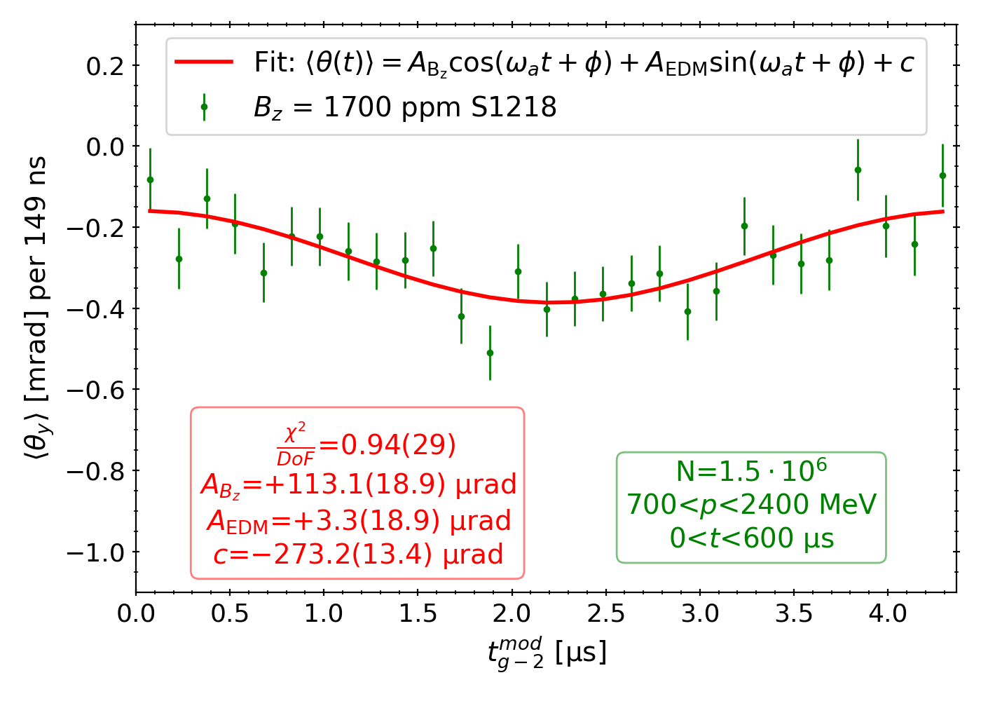

In data, a comparison was made between the blinding from Equation 10.16 and a \sayrandomised double blinding: . This procedure allowed an additional unknown signal, without revealing the original blinding.
10.5.2 Fitting in data
The fit of Equation 9.1 to the number of quality tracks is shown in Figure 10.10a. This plot is analogous to the \saywiggle plot in Figure 9.1, but with the time modulation of Equation 10.9 applied. The subsequent fit of Equation 10.15 to the vertical angle oscillation, using the value of from Figure 10.10a, is shown in Figure 10.10b, for tracks in a 100 MeV range.
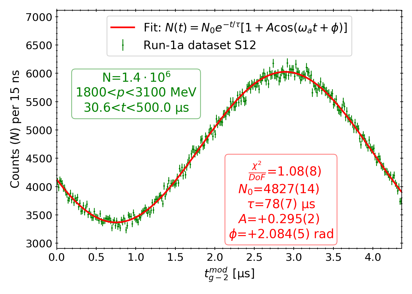
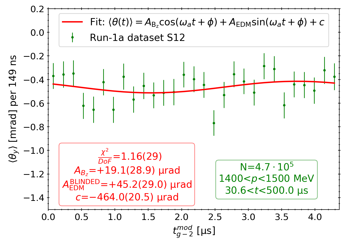
10.5.3 Momentum-binned analysis
The fit in Figure 10.10b is performed in a narrow momentum range (rather than a simultaneous fit to all data) due to a variation in the overall offset in the vertical angle () as a function of momentum, as demonstrated in Figure 10.11a. This is due to the vertical beam motion, discussed in Section 3.4. Negative is indicative of the centre of the beam being vertically lower than the centre of the detector. The global alignment effects were excluded as a cause, due to the two stations measuring the same variation in , while having different corrections from the alignment (see Table A.1).
Tracks of lower momentum exhibit an even more significant change in and therefore are not considered in this analysis. However, due to the optimal momentum cuts for this analysis (see Section 10.5.4.3), and the effect of dilution described in Section 10.5.5, the lowest and highest momentum tracks do not contribute significantly to the measurement of – regardless of the observed change in – and represent only a small population of all tracks (c.f. Figure 5.14).
Therefore, fits in individual momentum bins of 100 MeV are performed to measure , separately for each station and dataset, in the momentum range of 1100 MeV to 2300 MeV, as shown in Figure 10.11b for the Run-1d dataset.
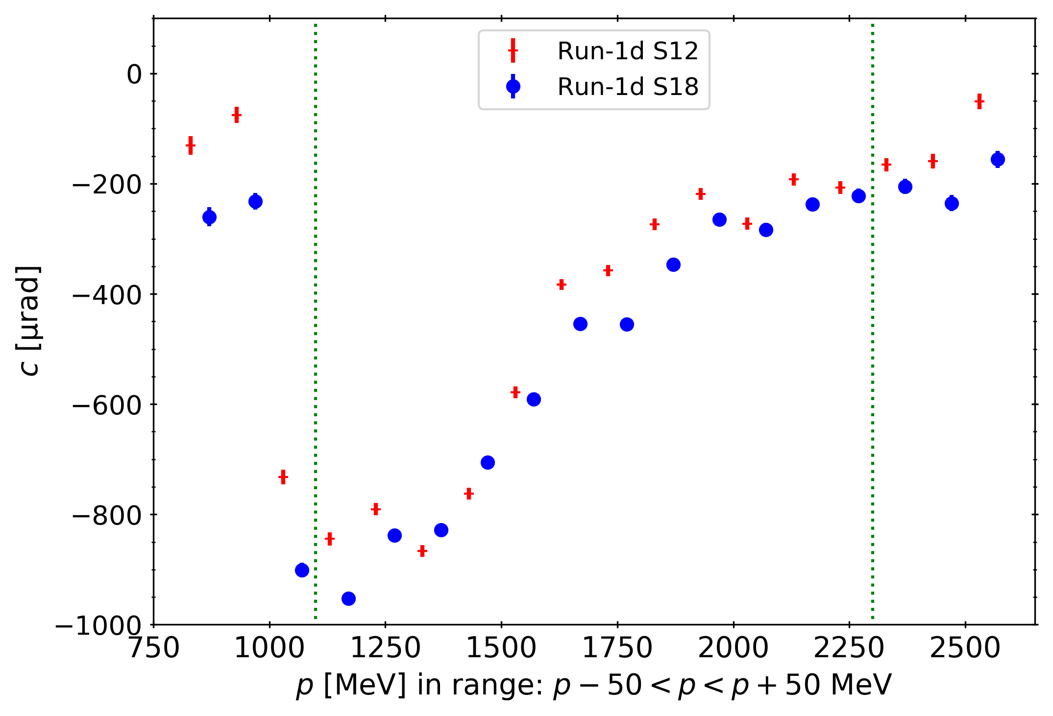
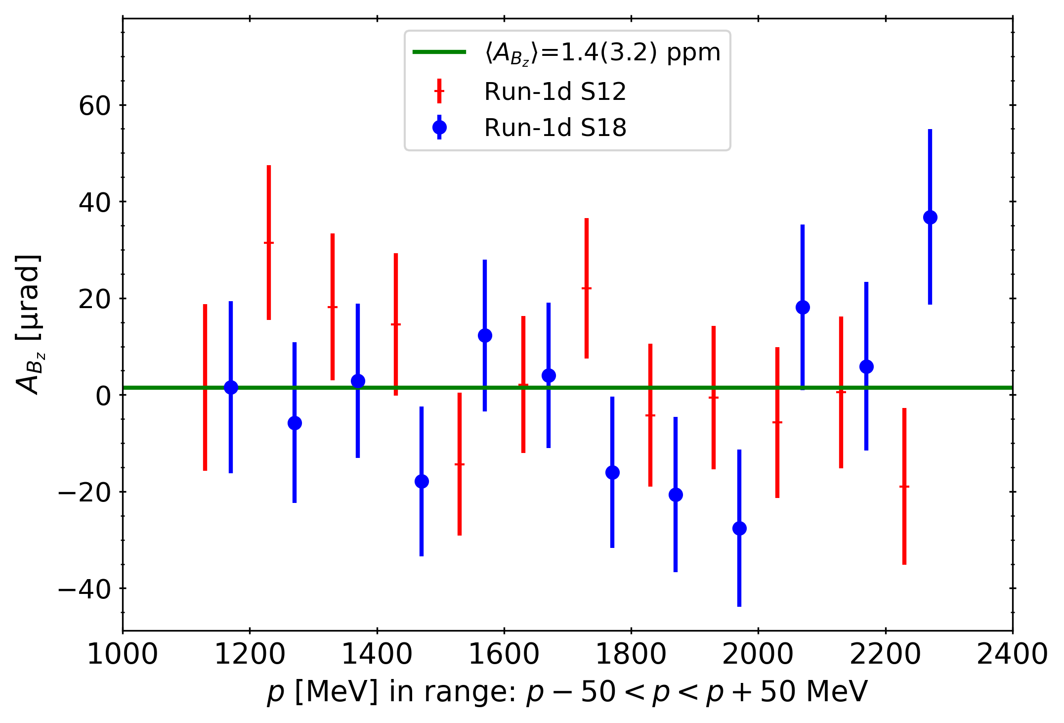
per dataset is determined as the uncertainty-weighted mean. The fitting results in the four Run-1 datasets are summarised in Figure 10.12a, while the equivalent results in 1999 and 2000 at the BNL [15] experiment are summarised in Figure 10.12b.
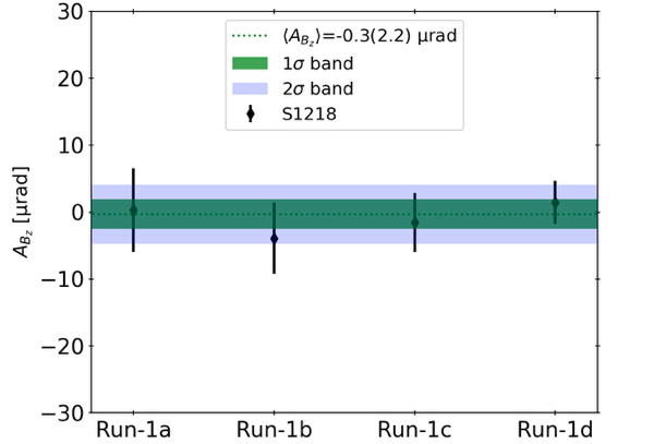
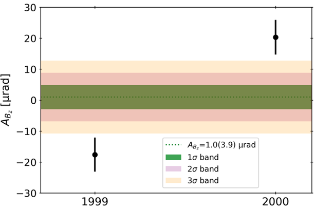
10.5.4 Optimising cuts selection
The results in Figure 10.10 were obtained with a particular choice of cuts: fit-start and end-times ( ) and momentum ( MeV MeV, for the number oscillation). Moreover, the analysis relied on a choice of the period (), as well as the phase () extracted from the fit of Equation 9.1. In this section, these choices will be motivated, and their stability assessed.
10.5.4.1 Dependence of fit on data subset
In order to assess the robustness of the fit, fits can be performed to different subsets of the data and the results compared. For example, varying the fit start-time, where data at a later start-time is a subset of data at an earlier time. The difference in a given fit parameter for the two datasets has an allowed difference, , where 2 denotes the smaller dataset and 1 the larger, is given by
| (10.17) |
This equation is valid for any fit function, regardless of the number of parameters and possible correlations among them [102]. The results for with different fit start-times are shown in Figure 10.13.
10.5.4.2 Fit start-time
First of all, a careful choice of the fit start-time is necessary – it should be a multiple of because data is modulated using Equation 10.9. This is demonstrated in Figure 10.14.
The second requirement is that the fit start-time must be greater than (see Section 3.3.3), and should be as low as possible to minimise the statistical uncertainty. A fit start-time of was therefore chosen, with the variation of at later fit start-times shown in Figure 10.13.

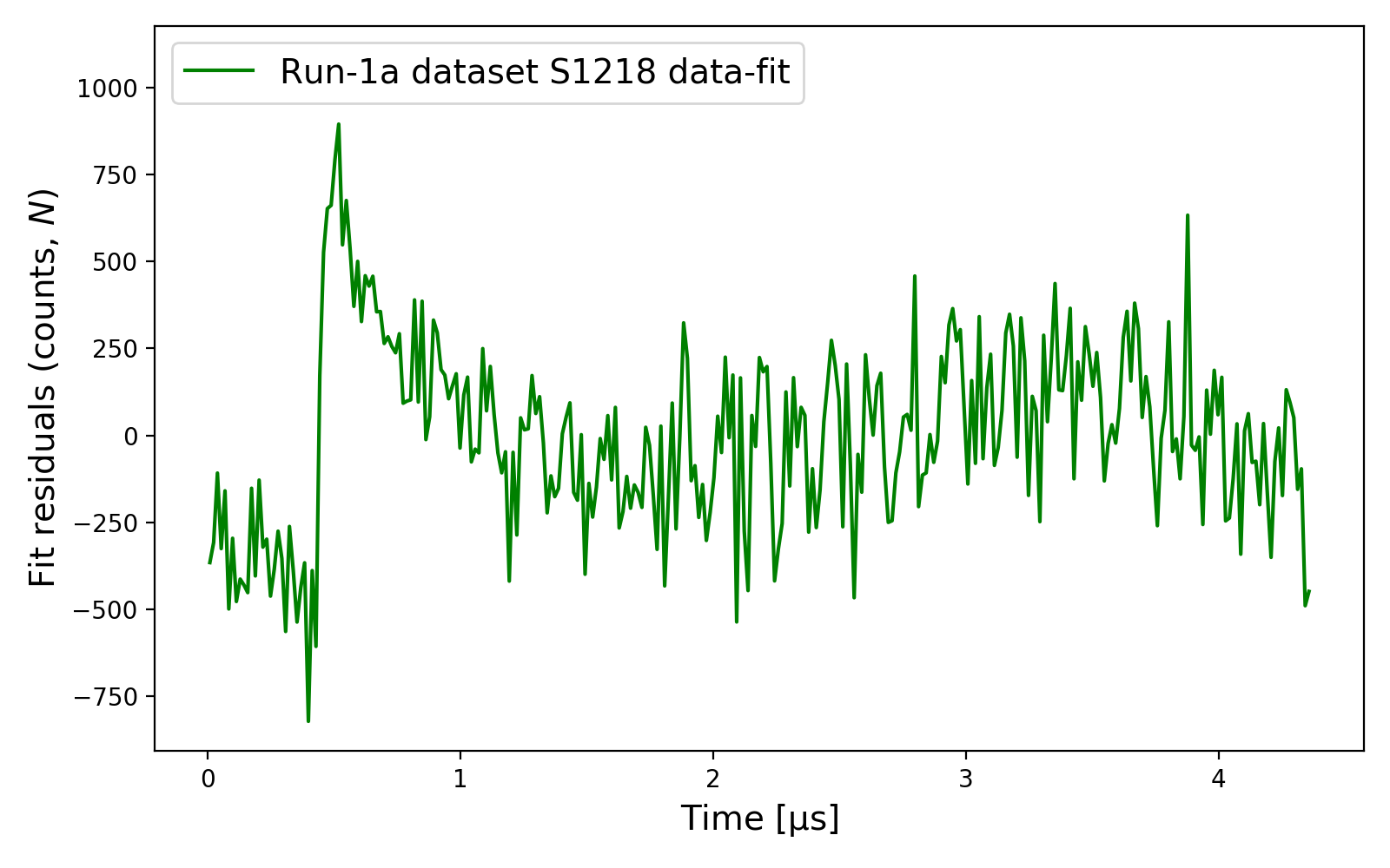
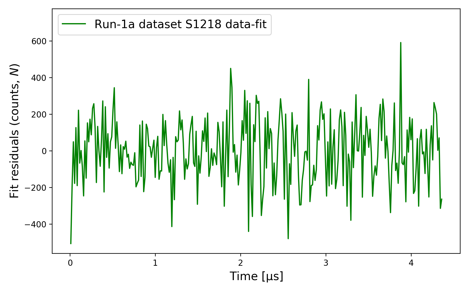
10.5.4.3 Momentum cuts
Equation 10.15 is fitted in momentum bins of 100 MeV due to the strong momentum dependence of . Using the simulation with a truth value of ppm, it was verified that a symmetric cut on momentum is more appropriate than an asymmetric one (see Section D.2), as shown in Figure 10.15.
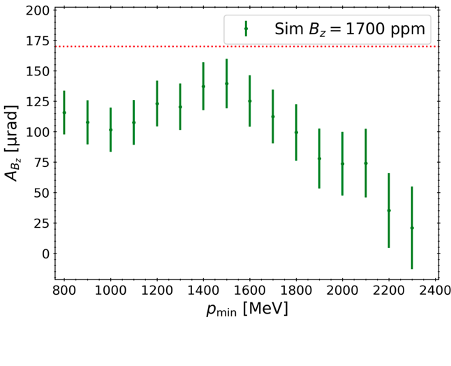
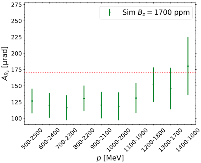
Tracks of higher momentum predominantly originate further away from a station, as seen in Figure 5.16b. Therefore, high momentum tracks with large angles () miss the tracker station – this can be thought of as a \saycone effect. As a consequence, the SD of () is narrower for higher momentum tracks, as compared with lower momentum tracks, as measured by the detectors. This is demonstrated in Figure 10.16.
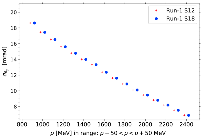
This effect directly leads to a reduction in the uncertainty of the parameter in the fit at high momentum, as shown in Figure 10.17a where each momentum bin has the same number of tracks.
However, considering a non-fixed number of tracks in each momentum bin results in the distribution shown in Figure 10.17b, where past 1600 MeV the is increasing with a deceasing number of tracks per bin.
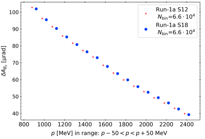
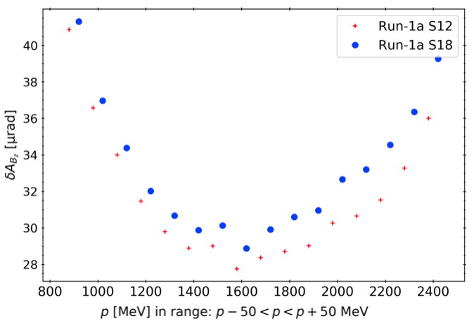
The mid-momentum tracks are thus the most sensitive in measuring . A momentum range of 1100 MeV to 2300 MeV is therefore used to fit Equation 10.15, with separate fits performed in 100 MeV momentum bins.
10.5.4.4 Assessment of period and phase
In order to modulate data using Equation 10.9, must be known a priori to a reasonable precision. Using the frequency MHz, as measured by the BNL experiment [1], yields the value of . This choice can be evaluated by changing by ppm to ppm and recording the change in , as shown in Figure 10.18a.
The small variations in Figure 10.18a imply that there is no real systematic effect there. However, extracting the slope of the fit allows an assessment of the magnitude of the systematic uncertainty from the choice of , as described in Section 10.5.4.5, to be made.
The change in due to the variation of is shown in Figure 10.18b.
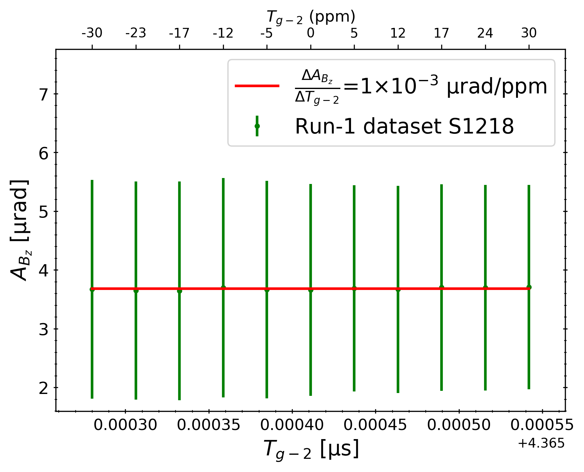

10.5.4.5 Systematic uncertainty evaluation
Small variations of due to the choices of and were observed. The systematic uncertainty for each, and the total systematic uncertainty, on are summarised in Table 10.1. Slopes from Figures 10.18a and 10.18b were used in the estimation, as well as the error from the fit on in Figure 10.10a. The total systematic uncertainty of was found to be negligible compared to the statistical uncertainty of (see Figure 10.12a).
| Systematic source | Value [] |
|---|---|
| Total |
10.5.5 Conversion of into
With the optimal cuts justified, and systematic effects on evaluated, it is now possible to convert the observed amplitude into . is related to the precession-plane tilt in the lab-frame, , in the same way as in Equation 10.5. However, given that the muon motion is along (c.f. Figure 10.5), there is no Lorentz boost in this direction. Therefore, an estimate of can be derived directly from the measured angle in the lab-frame
| (10.18) |
for which is the case. In Equation 10.18, is the asymmetry-dilution factor, analogous to in Equation 10.5. This asymmetry factor was estimated from the simulation, as shown in Figure 10.19a, where a parabolic function was fitted to the simulation data, given by
| (10.19) |
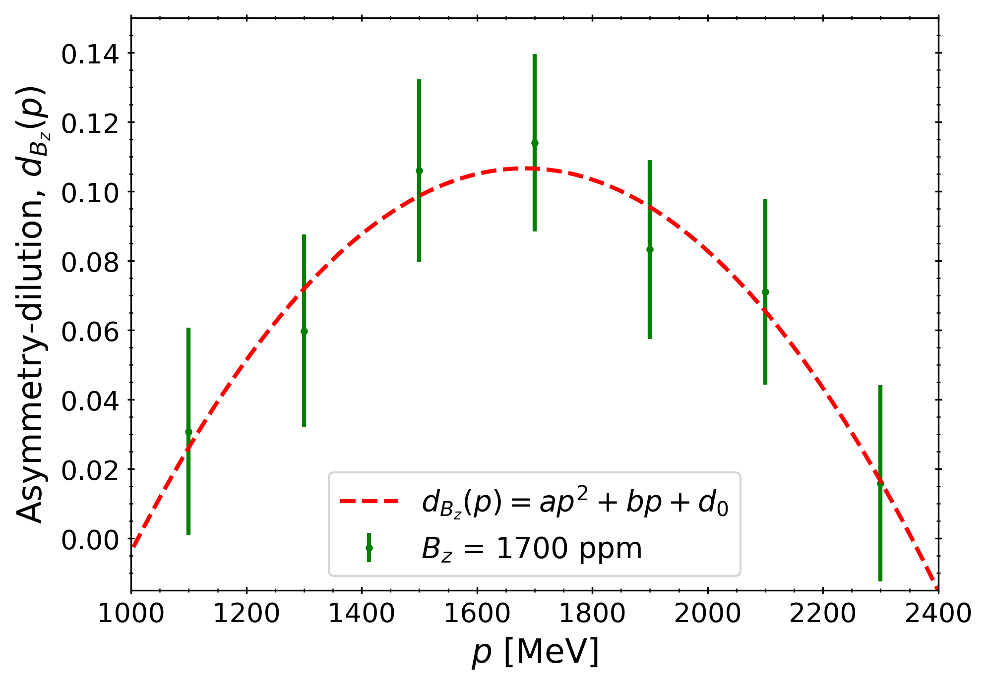
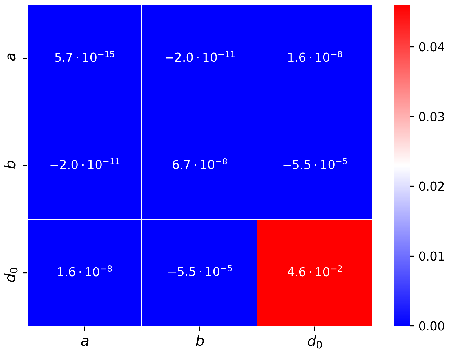
Finally, the uncertainty on in momentum bin is given by
| (10.20) |
where is the fit error (e.g. Figure 10.10b), and is computed using the variance of the parameters in Figure 10.19b.
Using Equations 10.18 and 10.20, the measured value of in each momentum bin in Figure 10.11b, and the value of from Equation 10.19, was estimated (per momentum bin), as shown in Figure 10.20.
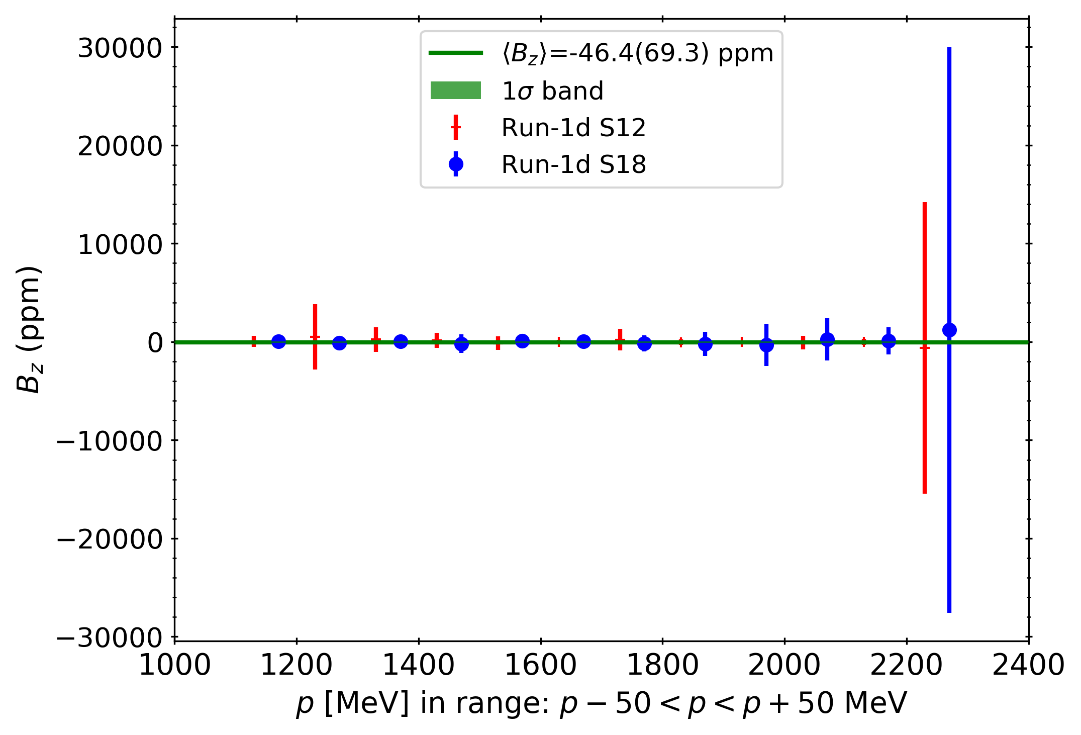
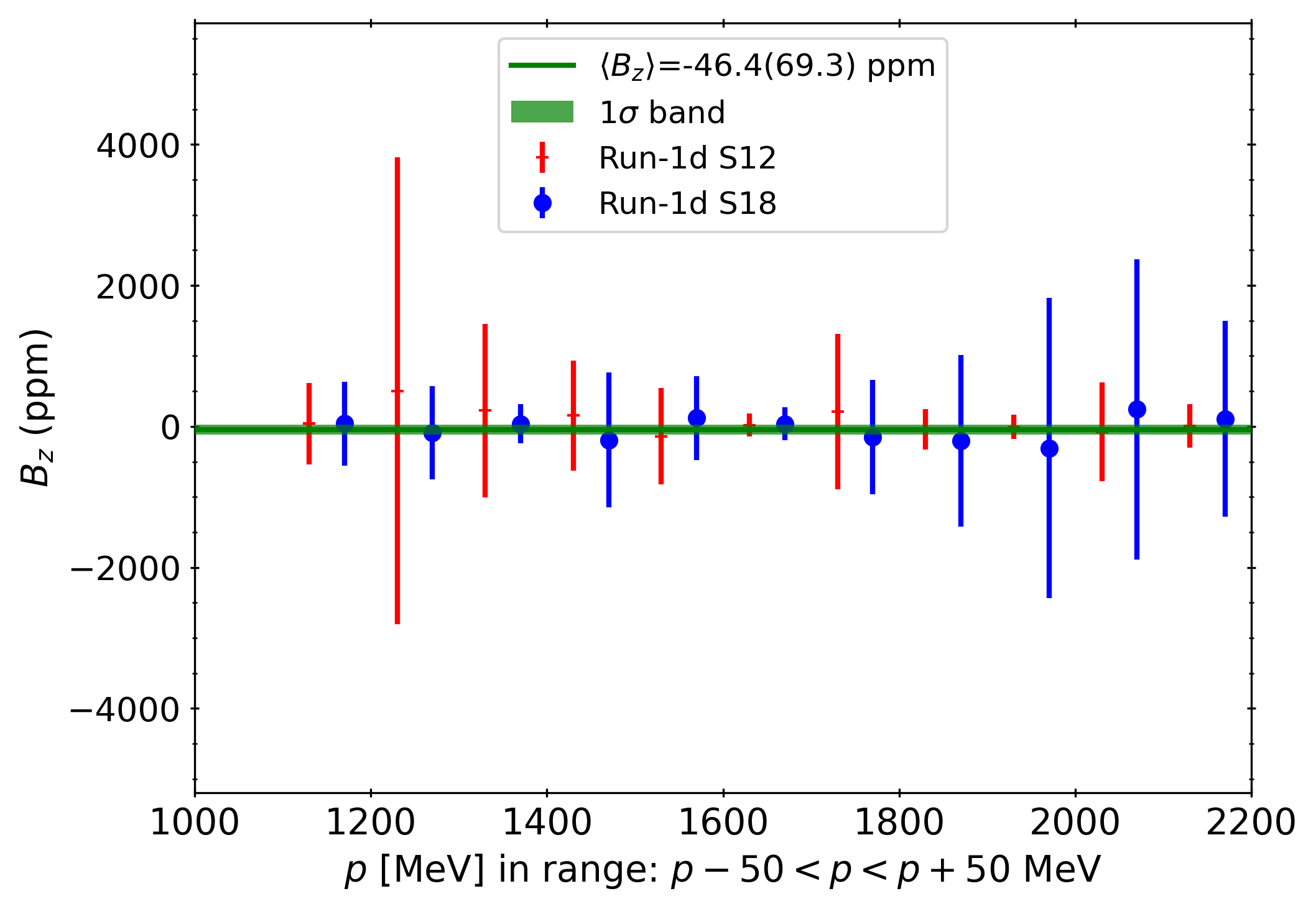
10.5.6 Analysis results
The measured values of from the four Run-1 datasets are summarised in Figure 10.21. The results from the individual datasets are compared to the mean Run-1 result of ppm, and are found to be in agreement to better than .
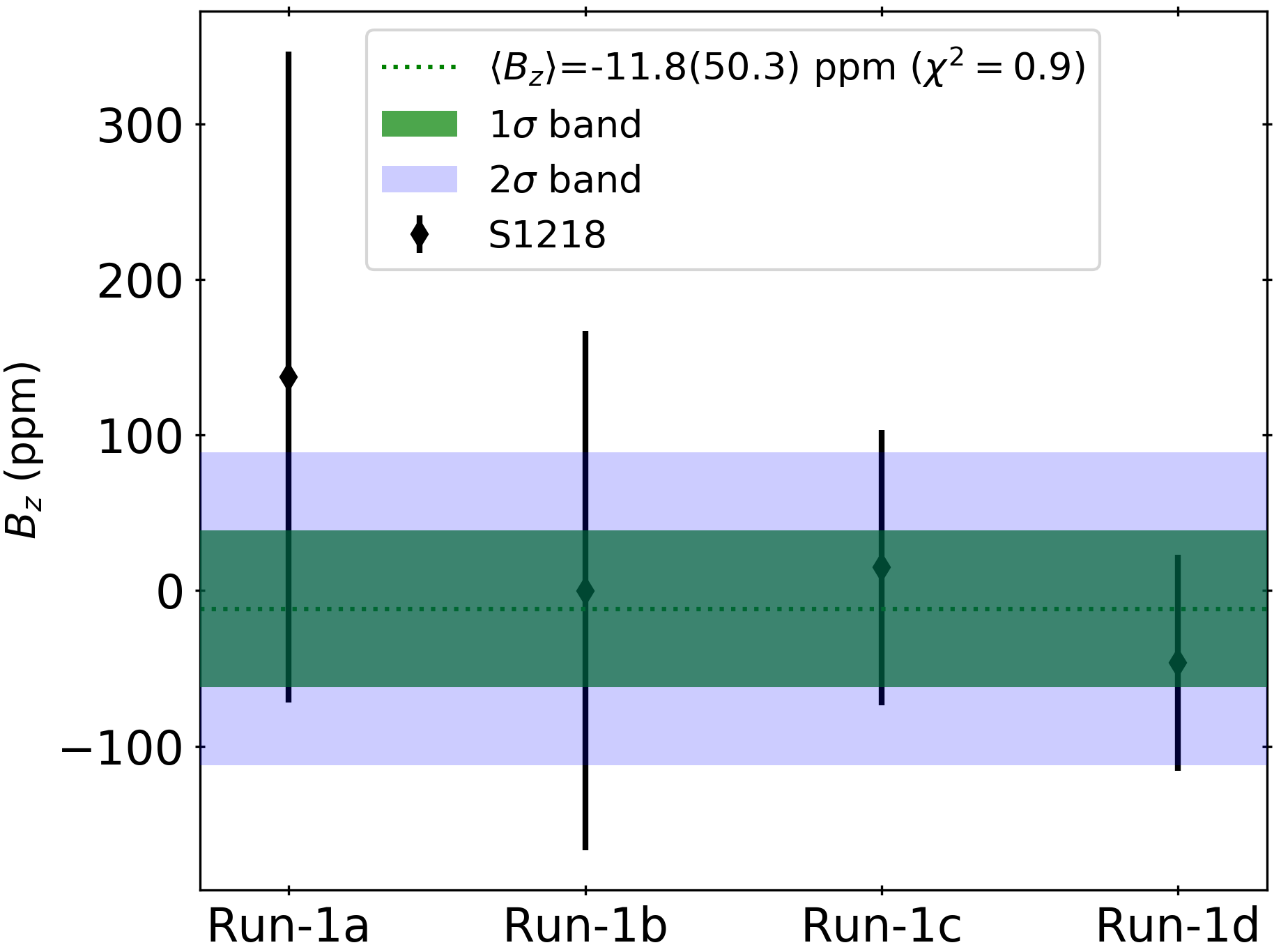
10.6 Outlook
The analyses presented in this chapter - measurements of and using the tracking detectors - were not attempted at the BNL experiment. The preliminary measurement of confirmed that such a technique is viable using the tracking detectors, and yielded a value of ppm in Run-2.
The measured value of in Run-1 is consistent with zero, with a precision of 50 ppm. Additionally, the measurement is in agreement with the direct measurement of ppm [96] before Run-1.
The precision ( ppm) will be improved with the increase in the number of reconstructed tracks by adding new data – Run-2 data-reconstruction is currently ongoing. Moreover, the track-reconstruction with an improved tracking efficiency is currently ongoing on the UK grid (see Section 3.8.2). The final precision is likely to reach 5 ppm by Run-5, as shown in Figure 10.22. This is more precise than the design goal of ppm, which would correspond to the uncertainty on of ppb [103].
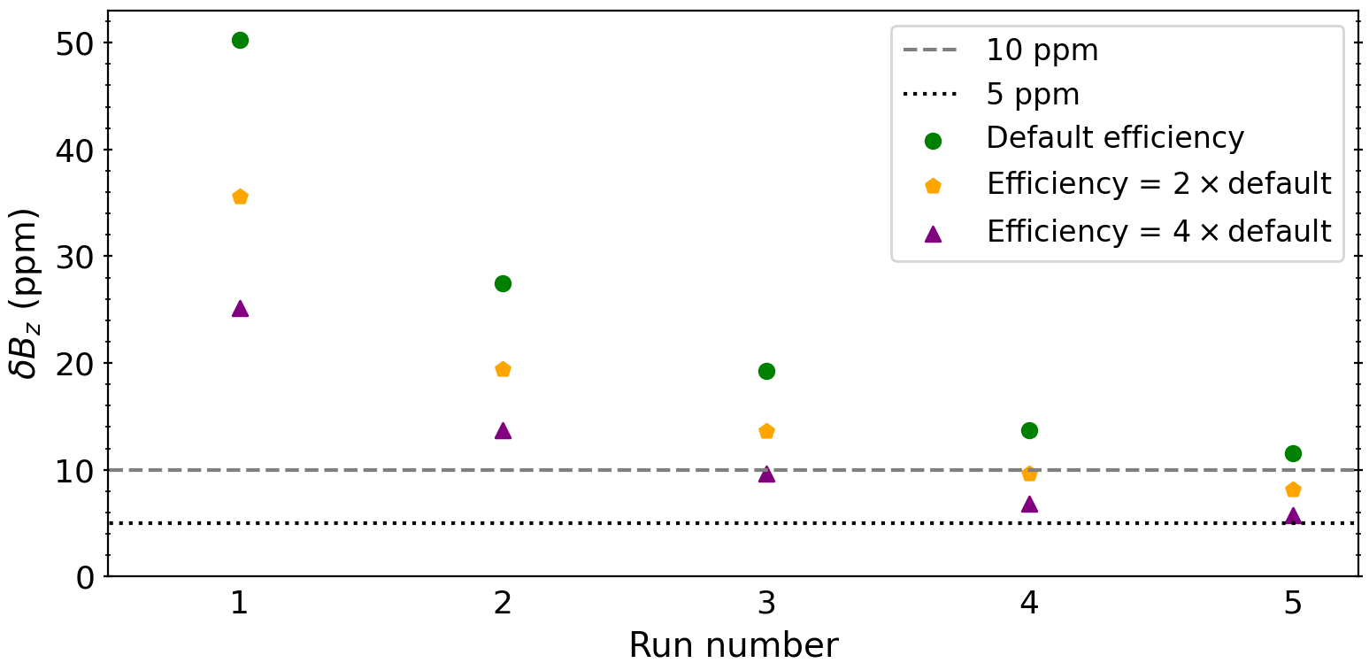
Chapter 11 Conclusions
The Fermilab Muon experiment will measure the muon magnetic anomaly, with a precision of 140 ppb, and will search for the muon EDM, with at least a factor of 10 improvement on the world’s best measurement. The three data-taking periods, Run-1, Run-2, and Run-3, have been completed, with preparations for Run-4 currently ongoing. Essential in reducing the systematic uncertainty on the measurement of are the straw tracking detectors, which perform track extrapolation backwards to the muon decay point and forwards to the calorimeters. Moreover, systematic effects, such as the vertical pitch, require a correction that is accessible via a measurement of the vertical width of the beam by the tracking detectors. The beam profile from the tracking detectors is also convoluted with the magnetic field map to find the field experienced by the muons at the point of decay.
In order to accurately reconstruct the beam profile, the tracking detectors must be correctly aligned. The alignment algorithms were validated using simulation, which converged after three iterations with () tracks to within radially and vertically. The track-based internal alignment was implemented with data from Run-1. The number of reconstructed tracks has increased by due to the position calibration from the alignment. Moreover, an improvement in the mean track of was achieved. After the alignment procedure, the uncertainty contribution from the tracker misalignment to the pitch correction is now negligible.
An alignment manual [3] allowing future alignment determinations, has been produced. The derived alignment constants were written into a PostgreSQL database, where each set of constants is associated with a given range of runs. Additionally, the stability of the alignment results was verified using Run-2 data.
A potential EDM of the muon would increase the observed signal and tilt the precession-plane of the muon. The tracking detectors will realise an EDM measurement through the direct detection of an oscillation in the average vertical angle of the positron from the muon decay. An observation of a muon EDM would be evidence of new physics and would provide a new source of CP violation in the charged lepton sector.
Essential in measuring the EDM, as well as , are accurate and precise estimations of potential non-zero radial and longitudinal magnetic fields, which can tilt the precession-plane of the muon. The radial and longitudinal magnetic fields were estimated using data from the tracking detector. A preliminary estimation of the radial field resulted in a value of ppm. An in-depth analysis of the vertical angle oscillation yielded a value of the longitudinal field consistent with zero: ppm. Moreover, the first analysis of with data from the tracking detector was made. The projected precision will allow an independent cross-check of the BNL and Fermilab Run-1 determinations of , using the Run-1 to Run-3 datasets from the tracking detector.
At the time of writing, the experiment-wide effort on the analysis of Run-1 data is nearing completion, with the announcement of the first result expected in the coming months. This could be a fascinating time for the scientific community: only time will tell if the measurement by the experiment will be the harbinger of new physics!
Appendix A Global alignment of the tracking detectors
This section on the global alignment briefly summarises the work done by Dr Horst Friedsam [104], Dr Leah Welty-Rieger [105] and Dr Joe Price [106].
The global alignment established an absolute position of the tracker stations relative to the rest of the experiment. This procedure consisted of two parts: physical survey measurements of the modules by the Alignment and Metrology Department at Fermilab, and the implementation of these measurements in the software framework.
A.1 Survey alignment
The first step in the survey of the tracker compared measurements of a single tracker module with the design model. Agreement was found within , with the survey points used in the comparison indicated in Figure A.1. The design model was then used to transform from a point in a local tracker coordinate system to the global coordinate system. As the tracker modules are mounted into a vacuum chamber, as shown in Figure 5.2, the global alignment requires the radial and vertical positions of the vacuum chambers to be determined. The measurements were performed using the API Laser Tracker as shown in Figure A.2. These measurements and the design model was then used to estimate the position of the module flange, the straws themselves, and the carbon fibre post, with the error on the estimated positions determined to be .
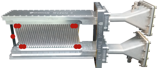
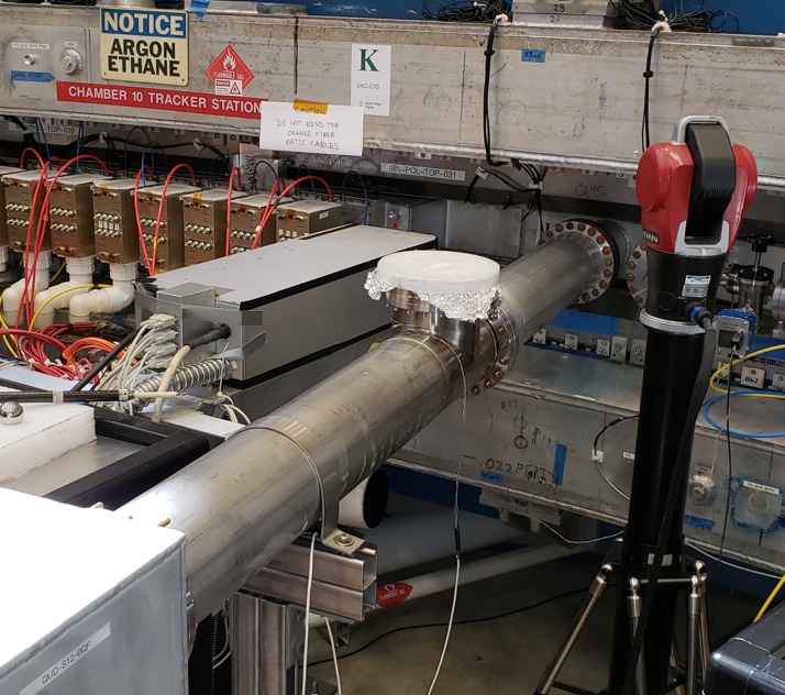
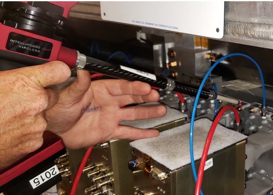
A.2 Global alignment in simulation
The survey measurements described above resulted in four global corrections per station: a radial translation, a vertical translation, a pitch (radial) rotation, and a roll (vertical) rotation, as summarised in Table A.1.
| vertical position [] | vertical angle [rad] | radial position [] | radial angle [rad] | |
|---|---|---|---|---|
| S12 | ||||
| S18 |
A comparison between the extrapolated beam position determined before and after the implementation of the global alignment is shown in Figure A.3 for the vertical position. After the alignment, one would not expect the radial or vertical beam distributions from the two stations to match exactly. This is the case due to the closed-orbit effect (see Section 3.4.5), as the two tracker stations see \saydifferent beams. The summary of the change in the vertical and radial extrapolated beam position after the global alignment is presented in Table A.2.
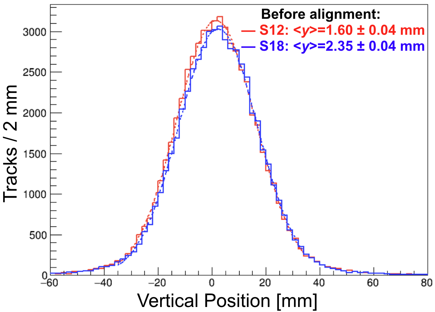

| vertical S12 [] | vertical S18 [] | radial S12 [] | radial S18 [] |
|---|---|---|---|
A.3 Global alignment uncertainty contribution
The Mahalanobis method [86] was used to estimate the uncertainty on the beam extrapolation arising from the uncertainty on the global alignment. Nine Mahalanobis points are derived from the two-parameter straight line-fit. The results from placing the modules in one of these nine positions and determining the extrapolated beam positions are shown in Figure A.4.
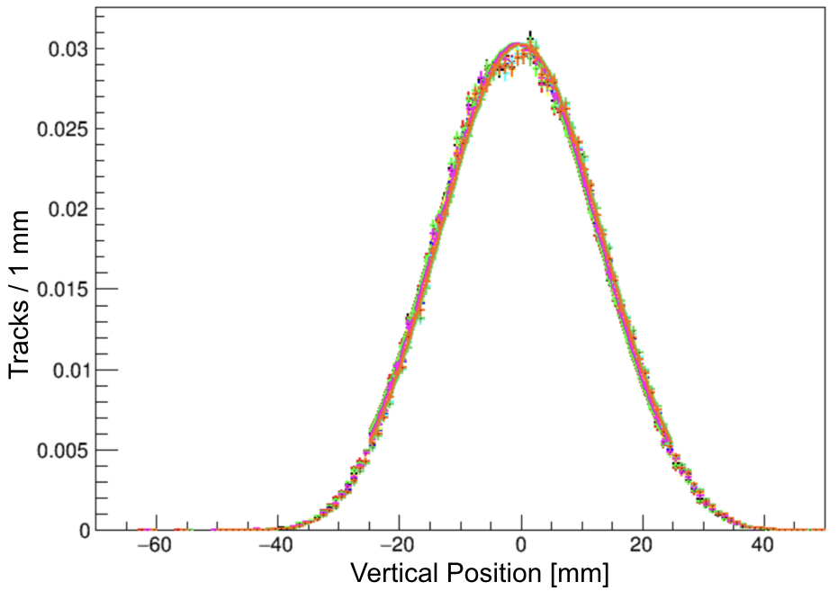
To estimate the uncertainty on the pitch correction from the global alignment, the largest vertical beam width of the eight cases in Figure A.4, relative to the nominal case, was used. This change () corresponds to mm. Using Equation 3.11 and the estimated leads to of ppb. This is negligible, compared to the total tracker pitch correction uncertainty of 8.6 ppb (in Run-1), as described in Section 3.4.1.
Appendix B Derivations of analytical equations for internal alignment
This section provides derivations of the equations used in Chapter 7.
B.1 Straight line-fit in 2D
Derivations of Equations 7.18 to 7.21, describing the effect of a translational misalignment on a line of best fit in 2D is given below, for a line of the form
| (B.1) |
where is a hit position (i.e. height) along an infinitesimally thin detector plane, and is a plane position along the direction of the beam. A residual, , on a detector plane is given by
| (B.2) |
with the , as a sum of all the residuals in planes, defined as
| (B.3) |
for a constant detector resolution, , and a special case of no misalignment and no smearing. The aim is to minimise with respect to line parameters and :
| (B.4) |
and
| (B.5) |
Without the loss of generality, one can define the \saycentre-of-mass of planes to lie at 0 along , so that , which simplifies the above equations to
| (B.6) |
and
| (B.7) |
For a realistic case of non-zero characteristic misalignment, , along , and smearing due to the detector resolution, , on a plane, one has a hit position defined by
| (B.8) |
where one can define two variables relating the truth (e.g. ) and measured line parameters due to the resolution and misalignment effects, substituting for the measured slope, , from Equation B.6 into Equation B.2
| (B.9) |
and similarly for the intercept
| (B.10) |
Using Equations B.8, B.9 and B.10 the residual in a plane can be defined as
| (B.11) |
It is now possible to derive an analytical form of the mean residual, in a detector layer , over tracks
| (B.12) |
where was used. The second term in Equation B.12 gives a hint of an effect of misalignment in other layers on the residual in a particular layer . The analytical form of the standard deviation of the distribution of residuals in a layer , over tracks is given by
| (B.13) |
Finally, an analytical equation for on a fit to a misaligned detector for tracks can be derived
| (B.14) |
The derived equations for , , and apply for a 2D case of a straight line-fit to a misaligned detector planes along , with a given detector resolution on hits. Nevertheless, the derived equations are quite instructive of the effect of misalignment, and give correct analytical predictions for a 2D toy-model, as shown in Figures 7.6, LABEL: and 7.7.
B.2 Residual derivatives with circle-fit in 2D
In the case of a circle-fit using straight tracks the residual, , is given by
| (B.15) |
with two local derivatives,
| (B.16) |
and
| (B.17) |
The action of an anticlockwise rotation is given by
| (B.18) |
The transformation back to the global coordinates is given by
| (B.19) |
The equation for a residual, under a 2D rotation, can be written using Equation B.19, and is given by
| (B.20) |
Ultimately, an expression for in terms of global and local parameters is used
| (B.21) |
This can be obtained using the chain rule
| (B.22) |
where represents a measurement (e.g. straw displacement in or ). Using Equation B.22 one can write the equation for the residual derivative expressed without the use of the truth parameters (i.e. )
| (B.23) |
at this point, a substitution from Equation B.19 can be used to simplify the expression to
| (B.24) |
where all inputs come either from measurements or assumption of the ideal geometry.
B.3 Residual derivatives in 3D
The straw wire can be parametrised as
| (B.25) |
as the position on the straw is constant with , and the slope in is due to the stereo angle on the straw wire, , of with . A geometrical approach can be taken to express the requirements on the DCA from Equation 7.27 as
| (B.26) |
which projects the distance between the intercept of the lines, to the normal, , between the two lines.
Using the track parametrisation from Equation 7.8 the DCA in 3D is given by
| (B.27) |
and the residual is simply
| (B.28) |
The four local derivatives , , , and are then given by:
For the \say-intercept
| (B.29) |
for the \say-intercept
| (B.30) |
The \sayslope (defined in Equation 7.10)
| (B.31) |
and
| (B.32) |
And the two global derivatives for radial and vertical translations are
| (B.33) |
and
| (B.34) |
The 3D rotation matrix is given by
| (B.35) |
where , and are the Euler angles. There are three possible rotations (see Figure 7.3) around the centre of the tracker module. A rotation around the -axis is the same as considered previously in Equation B.23, but needs to be extended to a 3D geometry. With the constraint that a point along the straw will have the same vertical height () before and after the above rotation with the derivatives for the anticlockwise rotation along the -axis given by
| (B.36) |
The global derivatives for the anticlockwise rotation along the -axis is
| (B.37) |
and similarly for the rotation along the -axis
| (B.38) |
and -axis
| (B.39) |
The fifth local derivative in the presence of a magnetic field is given by
| (B.40) |
The vector containing derivatives of the residuals with respect to the fitted track parameters is given by
| (B.41) |
Appendix C Control and steering of PEDE
This section summarises the steering and constraint options used in PEDE.
The PEDE steering file is given by
The constraint equation is given by
| (C.1) |
where is is the constraint value, is the global parameter label, is the parameter factor, and the summation is taken over the parameters contributing to the constraint. The constraints given in Section 7.3.4 can be written as the inputs to PEDE as follows:
-
1.
Constraint on the overall radial translation
(C.2) where, for example, label corresponds to station number 12, module number 8 and parameter number 1 (i.e. radial shift). The factor of simply means equal weighting for all parameters.
Equation C.2 is written in the PEDE format as follows
1! Radial translational fixing (no overall movement):2Constraint 031211 141221 151231 161241 171251 181261 191271 1101281 1 -
2.
Constraint on the overall vertical rotation
(C.3) 1! Vertical rotational constraint2! around the centre of the station:3Constraint 041212 751222 561232 371242 181252 -191262 -3101272 -5111282 -7 -
3.
Constraint on the radial bowing effect
(C.4) 1! Bowing effect: parabloic radial term2! describing the track curvature3! around the centre of the station:4Constraint 051211 4961221 2571231 981241 191251 1101261 9111271 25121281 49
Appendix D Ancillary analysis plots and derivations
This section contains accompanying plots and derivations to Chapters 9 and 10.
D.1 Ancillary wiggle plots
Wiggle plots and ten-parameter fits across the four datasets: Run-1a (Figure D.1), Run-1b (Figure D.2), Run-1c (Figure D.3), and Run-1d (Figure D.4).


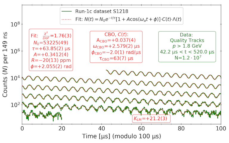
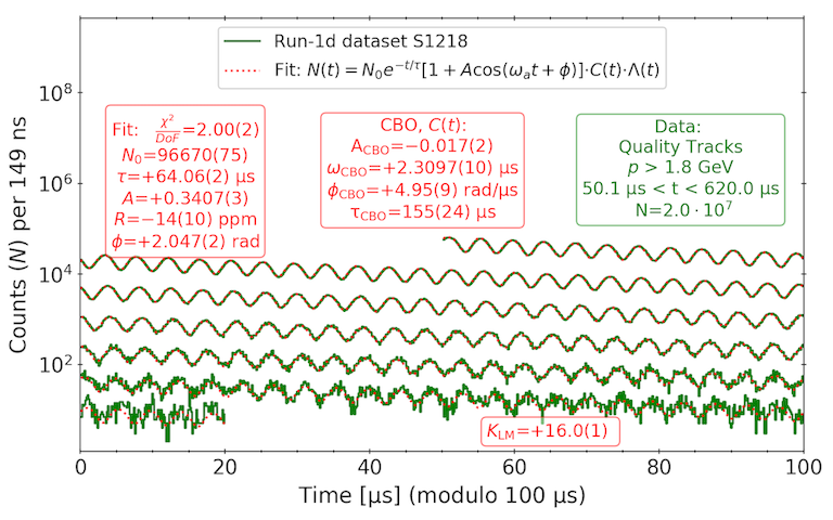
D.2 Momentum cuts used in the wiggle plots
Imposing a momentum cut, , on data in Figure 9.1 is motivated by the muon decay asymmetry () and the number of tracks () used in the fit, such that the optimal value of corresponds to the quantity reaching the maximum [102]. That is, the statistical uncertainty on (or ) is minimised when is maximised.
If the momentum fraction, , is defined to be
| (D.1) |
then, in the lab-frame, both and can be expressed [11] as
| (D.2) |
and
| (D.3) |
The above expressions are plotted in Figure D.5a. Analytically, the optimal asymmetric momentum cut () occurs at or MeV. This was empirically verified using the Run1-a dataset, with the optimal momentum cut determined in Figure D.5b.
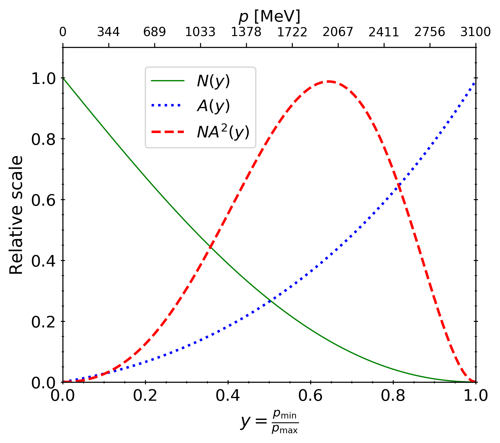
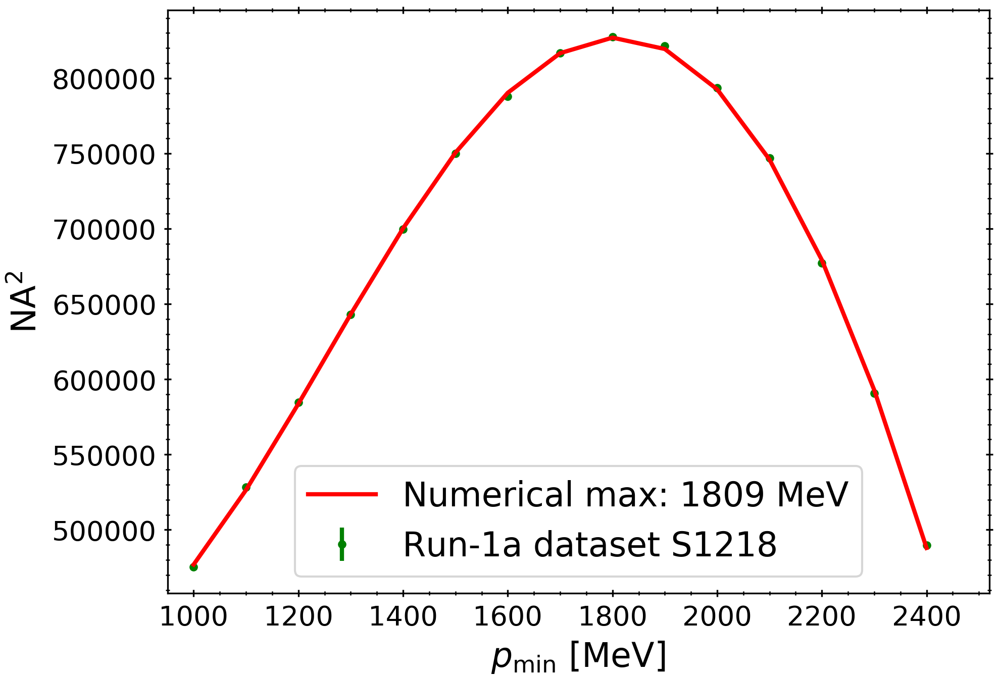
D.3 Lorentz boost of the tilt angle
The tilt angle of the muon spin precession-plane is reduced by the relativistic effect of length contraction [94]. This is demonstrated in Figure D.6.

The tilt angle, in the muon rest-frame, is given by
| (D.4) |
which, in the lab-frame, is equivalent to
| (D.5) |
and
| (D.6) |
These allow for the tilt angle in the lab-frame to be expressed as
| (D.7) |
Therefore,
| (D.8) |
References
- [1] G. Bennett et al., Final report of the Muon E821 anomalous magnetic moment measurement at BNL, Phys. Rev. D 73, 072003 (2006).
-
[2]
G. Lukicov,
EDM analysis with big-data, 10.5281/zenodo.3678580,
https://github.com/glukicov/EDMTracking (2019). -
[3]
G. Lukicov,
Tracker alignment manual,
http://gm2-docdb.fnal.gov/cgi-bin/ShowDocument?docid=9857 (2019). - [4] G. Lukicov, The straw tracking detectors, internal tracker alignment, and the muon EDM measurement, arXiv:1909.12900 (2019).
-
[5]
G. Lukicov,
Alignment of the tracking detectors,
10.5281/zenodo.3678572,
https://github.com/glukicov/alignTrack (2016). - [6] B. Roberts and Y. Semertzidis, Lepton dipole moments, World Scientific, (2010).
- [7] T. Aoyama et al., The anomalous magnetic moment of the muon in the Standard Model, arXiv:2006.04822 (2020).
- [8] A. Keshavarzi, The muon : the hadronic vacuum polarisation contributions, PhD thesis, University of Liverpool (2018).
- [9] M. Badziak and K. Sakurai, Explanation of electron and muon anomalies in the MSSM, J. High Energy Phys. 10, 24 (2019).
- [10] A. Czarnecki and W. Marciano, Muon anomalous magnetic moment: a harbinger for new physics, Phys. Rev. D 64, 013014 (2001).
- [11] J. Grange et al., Muon technical design report, arXiv:1501.06858 (2015).
- [12] F. Hoogeveen, The standard model prediction for the electric dipole moment of the electron, Nucl. Phys. B 341, 322 (1990).
- [13] K. Babu, B. Dutta, and R. Mohapatra, Enhanced electric dipole moment of the muon in the presence of large neutrino mixing, Phys. Rev. Lett. 85, 5064 (2000).
- [14] R. Chislett, The muon EDM in the experiment at Fermilab, EPJ Web of Conferences 118, 01005 (2016).
- [15] G. Bennett et al., An improved limit on the muon electric dipole moment, Phys. Rev. D 80, 052008 (2009).
- [16] D. Stratakis et al., Accelerator performance analysis of the Fermilab Muon Campus, Phys. Rev. Accel. Beams 20, 111003 (2017).
- [17] T. Stuttard, The development, testing and characterisation of a straw tracking detector and readout system for the Fermilab Muon experiment, PhD thesis, University College London (2017).
- [18] J. Kaspar et al., Design and performance of SiPM-based readout of PbF2 crystals for high-rate, precision timing applications, J. Instrum. 12, 1009 (2017).
- [19] M. Lancaster, The new FNAL Muon experiment, PoS 192, 041 (2013).
- [20] A. Anastasi et al., The laser control of the Muon experiment at Fermilab, Nucl. Instrum. Meth. A 842, 86 (2017).
- [21] J. Hempstead, Overview of the experiment, DocDB:18289 (2019).
- [22] J. Mohr, D. Newell, and B. Taylor, CODATA recommended values of the fundamental physical constants: 2014, Rev. Mod. Phys. 88, 035009 (2016).
- [23] O. Kim et al., Reduction of coherent betatron oscillations in a muon storage ring experiment using RF fields, arXiv:1902.02959 (2019).
- [24] Iconel 600 technical data, (High Temp), http://www.hightempmetals.com/techdata/hitempInconel600data.php (2015).
- [25] N. Froemming et al., Commissioning the superconducting magnetic inflector system for the Muon experiment, FERMILAB-CONF-18-462-AD-PPD (2018).
- [26] K. Badgley, Updates on the FNAL inflector, DocDB:11142 (2018).
- [27] A. Schreckenberger et al., New fast kicker results from the Muon E-989 experiment at Fermilab, FERMILAB-CONF-18-167-E (2018).
- [28] D. Rubin, Kicker progress, DocDB:1739 (2014).
- [29] J. George, The new Muon experiment at Fermilab, DocDB:12212 (2018).
- [30] W. Wu and B. Quinn, Beam dynamics in storage ring, FERMILAB-CONF-17-667-PPD (2017).
- [31] J. Mott, Pitch: Path to Run-1, DocDB:21071 (2020).
- [32] A. Oppenheim, R. Schafer, and J. Buck, Discrete-time signal processing, Prentice Hall, (1999).
- [33] J. Mott, CBO frequency, elog:168 (2019).
- [34] T. Halewood-Leagas, Measurement of vertical betatron oscillations using the straw tracking detectors for the E989 Muon experiment at Fermilab, PhD thesis, University of Liverpool (2019).
- [35] A. Chapelain, Fast rotation status of the and Fourier methods, DocDB:18097 (2019).
- [36] J. Grange, Shift in due to couplings between longitudinal and transverse magnetic field inhomogeneities (distortion of the closed orbit), DocDB:2548 (2019).
- [37] J. Crnkovic et al., Lost muon study for the Muon experiment at Fermilab, IPAC-2017-WEPIK119 (2017).
- [38] R. Osofsky, Surface coil status, DocDB:11004 (2018).
- [39] R. Osofsky, Magnetic field status, DocDB:12473 (2018).
- [40] M. Smith, Developing the precision magnetic field for the E989 Muon experiment, PhD thesis, University of Washington (2017).
- [41] A. Fienberg, Measuring the precession frequency in the E989 Muon experiment, PhD thesis, University of Washington (2019).
- [42] M. Lancaster, Run-3 performance and comparison to Run-1 and Run-2, DocDB:21126 (2020).
- [43] K. Siang, How each dataset is different for Run-1 of E989?, DocDB:15781 (2019).
- [44] R. Fatemi et al., Data production for the Muon experiment, DocDB:4638 (2016).
- [45] K. Herner et al., Advances in grid computing for the fabric for frontier experiments project at Fermilab, J. Phys. Conf. Ser. 898, 052026 (2017).
- [46] K. Chadwick et al., FermiGrid — experience and future plans, J. Phys. Conf. Ser. 119, 052010 (2008).
- [47] R. Pordes et al., The Open Science Grid status and architecture, J. Phys. Conf. Ser. 119, 052028 (2008).
- [48] F. Gray, Subrun-level data quality control, DocDB:14962 (2018).
- [49] G. M. Kurtzer, V. Sochat, and M. W. Bauer, Singularity: Scientific containers for mobility of compute, PLOS ONE 12, 20 (2017).
- [50] C. Green et al., The art framework, J. Phys. Conf. Ser. 396, 022020 (2012).
- [51] R. Brun and F. Rademakers, ROOT - an object oriented data analysis framework, Nucl. Instrum. Meth. A 389, 81 (1997).
- [52] S. Agostinelli et al., Geant4: a simulation toolkit, Nucl. Instrum. Meth. A 506, 250 (2002).
- [53] L. Welty-Rieger, Using 3D engineering models in a Geant4 simulation, DocDB:4498 (2016).
- [54] W. Gohn, Data acquisition for the new Muon experiment at Fermilab, J. Phys. Conf. Ser. 664, 082014 (2015).
- [55] S. Ritt and P. A. Amaudruz, New components of the MIDAS data acquisition system, IEEE Conf. Proc. 1, 116 (1999).
- [56] L. Gibbons, CCC shutdown tasks, DocDB:7346 (2017).
- [57] D. Sweigart, A measurement of the anomalous precession frequency of the positive muon, PhD thesis, Cornell University (2020).
- [58] J. Mott, The readout system for the Fermilab Muon straw tracking detectors, PoS 282, 1163 (2017).
- [59] M. Pesaresi et al., The FC7 AMC for generic DAQ and control applications in CMS, J. Instrum. 10, C03036 (2015).
- [60] MicroTCA chassis with 12 AMC full size slots – VT891, (Vadatech), http://www.vadatech.com/media/VT891_VT891%20Datasheet.pdf (2015).
- [61] C. Hill, AMC13 XG operational specification, http://ohm.bu.edu/~chill90/op_specs/AMC13_Operational_Spec_05_13_2013.pdf (2012).
- [62] W. Turner, The construction and commissioning of the straw tracking detector in the new muon experiment at Fermilab, PhD thesis, University of Liverpool (2018).
- [63] T. Albahri, Construction and commissioning of straw tracking detectors for the E989 Muon experiment at Fermilab, PhD thesis, University of Liverpool (2019).
- [64] J. Grange, Trolley run videos, DocDB:5721 (2017).
- [65] G. Hesketh, R vs t calibration, DocDB:12227 (2018).
- [66] N. Kinnaird, Muon spin precession frequency extraction and decay positron track fitting in Run-1 of the Fermilab Muon experiment, PhD thesis, Boston University (2020).
- [67] V. Innocente and E. Nagy, Trajectory fit in presence of dense materials, Nucl. Instrum. Meth. A 324, 297 (1993).
- [68] S. Charity, Beam profile measurements using the straw tracking detectors at the Fermilab muon experiment, and a study of their sensitivity to a muon electric dipole moment, PhD thesis, University of Liverpool (2018).
- [69] C. Runge, Ueber die numerische Auflösung von Differentialgleichungen, Mathematische Annalen 46, 167 (1895).
- [70] J. Mott, Track quality cut service, DocDB:16444 (2019).
- [71] J. Bono and S. Charity, Muon-weighted field average, DocDB:19796 (2019).
- [72] G. Hesketh, Efficiency, DocDB:21705 (2020).
- [73] V. Blobel, Software alignment for tracking detectors, Nucl. Instrum. Meth. A 566, 5 (2006).
- [74] V. Blobel, Linear least squares fits with a large number of parameters, http://www.desy.de/~blobel/Mptwo.pdf (2007).
- [75] S. Borghi et al., First spatial alignment of the LHCb VELO and analysis of beam absorber collision data, Nucl. Instrum. A 618, 108 (2010).
- [76] T. Bilka, The beam test measurements of the Belle II vertex detector modules, J. Instrum. 12, C03002 (2017).
- [77] G. Flucke et al., CMS silicon tracker alignment strategy with the Millepede-II algorithm, J. Instrum. 3, P09002 (2008).
- [78] P. Schleper, G. Steinbrück, and M. Stoye, Alignment of the CMS silicon tracker using Millepede-II, J. Phys. Conf. Ser. 119, 032040 (2008).
- [79] D. Klopping, Development of a software-based detector alignment method for high resolution positron emission tomography scanners, PhD thesis, RWTH Aachen University (2014).
- [80] V. Blobel and C. Kleinwort, A new method for the high-precision alignment of track detectors, arXiv:hep-ex/0208021 (2002).
- [81] C. Kleinwort, Track fitting and alignment for a TPC with general broken lines, PUBDB-2014-04486 (2014).
- [82] S. Chatrchyan et al., Alignment of the CMS tracker with LHC and cosmic ray data, J. Instrum. 9, P06009 (2014).
- [83] J. Price, Tracker module swaps, DocDB:19279 (2019).
- [84] S. Foster, Tracker scattering target, DocDB:20222 (2019).
- [85] A. Luca, The Kalman filter algorithm for the tracking software, DocDB:20156 (2019).
- [86] P. Mahalanobis, On the generalized distance in statistics, Proceedings of the National Institute of Sciences (Calcutta) 1, 49 (1936).
- [87] G. Sweetmore, t0 and angular distribution, DocDB:19970 (2019).
- [88] S. Grant, Low DCAs, DocDB:20168 (2019).
- [89] J. Cooley and J. Tukey, An algorithm for the machine calculation of complex Fourier series, Math. Comp. 19, 297 (1965).
- [90] J. Price, CBO, DocDB:12933 (2018).
- [91] J. Erler, On the combination procedure of correlated errors, arXiv:1507.08210 (2015).
- [92] F. Gray, Run-2C DQC update, DocDB:22708 (2020).
- [93] M. Lancaster, Personal communication (2020).
- [94] J. Price and S. Charity, EDM simulation status, DocDB:4183 (2016).
- [95] M. Sossong, A search for an electric dipole moment of the positive muon, PhD thesis, University of Illinois at Urbana-Champaign (2005).
- [96] R. Osofsky, Magnetic field determination for Run-1 of the Fermilab Muon Experiment, PhD thesis, University of Washington (2019).
- [97] J. Price, EDM summary, DocDB:21509 (2020).
- [98] M. Syphers, Closed-orbit errors, DocDB:12197 (2018).
- [99] J. Mott and S. Charity, Radial field: measuring using quads, DocDB:19159 (2019).
- [100] B. Kiburg, Radial fields and EDM, DocDB:18685 (2019).
- [101] M. Fertl, Hall probe hardware requirements, DocDB:17596 (2019).
- [102] G. Bennett et al., Statistical equations and methods applied to the precision muon experiment at BNL, Nucl. Instrum. Meth. A 579, 1096 (2007).
- [103] W. Morse, Y. Semertzidis, and V. Tishchenko, Geometric phase systematic error, DocDB:1819 (2014).
- [104] H. Friedsam, Alignment results, DocDB:5955 (2017).
- [105] L. Welty-Rieger, Alignment studies, DocDB:15322 (2018).
- [106] J. Price, Tracker global alignment, DocDB:16063 (2019).