A Parallel Direct Eigensolver for Sequences of Hermitian Eigenvalue Problems with No Tridiagonalization

Abstract.

In this paper, a Parallel Direct Eigensolver for Sequences of Hermitian Eigenvalue Problems with no tridiagonalization is proposed, denoted by PDESHEP, which combines direct methods with iterative methods. PDESHEP first reduces a Hermitian matrix to its banded form, then applies a spectrum slicing algorithm to the banded matrix, and finally computes the eigenvectors of the original matrix via backtransform. Therefore, compared with conventional direct eigensolvers, PDESHEP avoids tridiagonalization, which consists of many memory-bounded operations. In this work, the iterative method in PDESHEP is based on the contour integral method implemented in FEAST. For the symmetric self-consistent field (SCF) eigenvalue problems, PDESHEP can be on average $1.25\times$ faster than the state-of-the-art direct solver in ELPA when using $4096$ processes. Numerical results are obtained for dense Hermitian matrices from real applications and large real sparse matrices from the SuiteSparse collection.

1. Introduction

Large-scale Hermitian eigenvalue problems arise in many scientific computing applications (e.g. condensed matter (Kohn, 1999), thermoacoustics (Salas et al., 2015)). In the case of electronic structure calculations based on Kohn-Sham density functional theory, a large nonlinear eigenvalue problem is iteratively solved through the self-consistent field (SCF) procedure, in which a sequence of related linear eigenvalue problems needs to be solved. Depending on the discretization method and basis used, the matrices can be sparse, dense or banded. In this work, we focus on the dense case. Dense eigenvalue problems are usually solved by using direct methods, and famous packages include ScaLAPACK (Blackford et al., 1997), ELPA (Marek et al., 2014), EigenExa (Imamura et al., 2011), etc. When solving sequences of related eigenvalue problems, these eigensolvers cannot exploit any knowledge of the properties of the problem, and thus they solve each problem of the sequence in complete isolation.

Compared to direct methods, one advantage of iterative methods is that the approximate eigenvectors from previous SCF iterations can be used as the initial guess to improve the convergence rate of subspace iterations (SI) for the current SCF iteration. Based on SI accelerated by Chebyshev polynomials, an efficient eigensolver (ChASE) has been proposed for sequences of dense Hermitian eigenvalue problems (Winkelmann et al., 2019). Compared to Elemental’s direct eigensolver (Poulson et al., 2013), ChASE is faster when computing a small portion of the extremal spectrum. ChASE becomes slower when computing a large number of eigenpairs (Winkelmann et al., 2019). It is also a common problem for other iterative methods such as the implicitly restarted Lanczos algorithm (Lehoucq et al., 1998) and LOBPCG (Knyazev, 2001), since they have to solve a projected dense eigenvalue problem as a part of the Rayleigh-Ritz procedure.

When computing a large number of eigenpairs with iterative algorithms, the most common approach is the spectrum slicing technique (Bai et al., 2000; Saad, 2011), that tries to compute the eigenvalues by chunks. Often, spectrum slicing is based on the shift-invert spectral transformation, which involves costly matrix factorizations. Some related works include (most of them are for sparse eigenproblems):

1. The shift-invert Lanczos method (SI-Lanczos). It was the default choice for spectrum slicing methods (Aktulga et al., 2014; Grimes et al., 1994) and has been used in SIPs (Zhang et al., 2007), SLEPc (Campos and Roman, 2012), and SIESTA-SIPs (Keçeli et al., 2016; Keçeli et al., 2018).

2. Polynomial filtering based method. It uses matrix polynomial filters to amplify the spectral components associated with the interested eigenvalues (Banerjee et al., 2016; Li et al., 2016), avoiding matrix factorizations, and packages include EVSL (Eigenvalue Slicing Library) (Li et al., 2019) and ChASE (Winkelmann et al., 2019).

3. Contour integral based method, where a matrix factorization is required at each integration point. The well-known packages include FEAST (Kestyn et al., 2016; Polizzi, 2009; Peter Tang and Polizzi, 2014) and z-Pares (Sakurai and Sugiura, 2003; Sakurai and Tadano, 2007).

4. The shift-invert subspace iteration method. A new method (SISLICE) is recently proposed in (Williams-Young et al., 2020) which combines shift-invert subspace iteration with spectrum slicing.

Iterative methods are rarely involved to solve dense Hermitian eigenvalue problems since both dense matrix vector multiplication and solving a dense linear system are considerably expensive. In this paper, iterative methods are combined with direct methods in a novel way. The central idea is that iterative methods are applied on a banded matrix with small bandwidth (usually less than $64$) instead of the original matrix. Then, iterative methods can be used to compute partial or full eigendecomposition of a dense Hermitian or symmetric matrix. It is a new framework for solving dense Hermitian eigenvalue problem, and will be named PDESHEP in this paper, short for a Parallel Direct Eigensolver for Sequences of Hermitian Eigenvalue Problems with no tridiagonalization.

The classical direct methods consist of three steps, see Fig. 1 for the main procedure. First, a dense matrix is reduced to its tridiagonal form via orthogonal transformations. One efficient reduction algorithm for tridiagonalization is the two-step approach (Bischof et al., 1994), which first reduces a dense matrix to band form and then further reduces it to a tridiagonal matrix. The symmetric band reduction (SBR) from band to tridiagonal fully consists of memory-bound operations, and its scalability is limited. Then, the eigendecomposition of tridiagonal matrix is computed by classical algorithms and finally the eigenvectors are computed via backtransform. The details are introduced in the next section. The starting point of this work is trying to get around SBR and propose a more efficient algorithm to solve a symmetric banded eigenvalue problem. From the results of Example 1 in section 4, we see that step (II) takes about half of total time when using many processes. It is better to replace step (II) by a more efficient and faster solver.

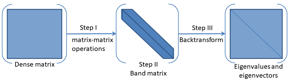
The procedure of our algorithm

Figure 1. The main steps of direct methods when using two-step symmetric banded reduction.

Many eigenvalue algorithms have been proposed for symmetric banded matrices. The most commonly used one is to reduce the banded matrix to tridiagonal form and then apply the DC, QR or MRRR (Dhillon et al., 2006) algorithms to it, just as done in ELPA (Auckenthaler et al., 2011). Some works suggest to use the banded DC algorithm (Arbenz, 1992; Gansterer et al., 2002; Liao et al., 2016) when the bandwidth is small, which requires more floating point operations. Just as shown in (Li et al., 2021b), the banded DC algorithm is slower than ELPA when the bandwidth is large. Another completely different approach is to use iterative methods. In this work, we apply the spectrum slicing methods to the symmetric banded matrix instead of the original full (dense) matrix. Since the semibandwidth of the intermediate banded matrix is very small, $n_{bw}=64$, it is very cheap to solve a banded linear system. Our method is similar to (Williams-Young et al., 2020; Zhang et al., 2007), but the matrix in our problem is banded, which makes the linear systems easy to solve. Similarly to previous methods (SIESTA-SIPs, SISLICE, ChASE), our algorithm is designed for SCF eigenvalue problems, and prior knowledge of eigenvalues and eigenvectors are used for spectrum partition and as initial vectors, respectively. The main advantage of PDESHEP is that it is suitable for many eigenpairs of dense matrices, not only for sparse matrices.

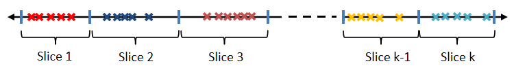
Figure 2. Partitioning of the spectrum with local clusters.

For spectrum slicing algorithms, the spectrum partition is very important for efficiency and robustness. It relates to load balance and the orthogonality of computed eigenvectors. The ideal case is that every slice has nearly the same number of eigenvalues and the gaps between eigenvalues in different slices are large, as shown in Fig. 2. Since we are dealing with self-consistent field (SCF) eigenvalue problems, we assume the prior knowledge of eigenvalue distributions is known. Otherwise, the spectral density estimation (also known as density of states or DOS) (Lin et al., 2016) and Sylvester’s inertia theorem (Sylvester, 1852) can be used to estimate or compute the distribution of eigenvalues of a banded matrix. In this work, we use a simplified k-means algorithm to partition the spectrum, that exploits the one dimensional structure of eigenvalues which are stored increasingly. Therefore, the simplified version requires much fewer operations than the general k-means algorithms. We first partition eigenvalues equally into $K$ groups and use their centers as the initial conditions of our simplified k-means algorithm, where $K$ is the number of partitioned slices. We find that this initialization method for k-means algorithms usually leads to a more ‘balanced’ partition, i.e, the variance of the number of eigenvalues in all slices is small. The simplified k-means algorithm is introduced in section 3.1.

To combine direct methods with iterative methods, we need some efficient data redistribution routines since the direct methods such as in ScaLAPACK and ELPA store matrices in 2D block cyclic data distribution (BCDD) while the iterative methods such as in FEAST store matrices in 1D block data distribution (BDD). We need two efficient data redistribution algorithms. One is used to redistribute a banded matrix in BCDD to 1D compact form as in LAPACK. The other one is used to redistribute a dense matrix stored in irregular 1D BDD to 2D BCDD with given block size $n_{b}$. By irregular we mean different processes may have different number of block rows or columns. None of BLACS routines works for the irregular case. We used the data redistribution algorithm proposed in (Li et al., 2021a). For the case that BLACS fits, the new data redistribution algorithm can be more than $10\times$ faster than the BLACS routine PXGEMR2D.

PDESHEP can be seen as a new framework of direct methods, and it can be combined with any spectrum slicing methods such as FEAST, SIPs or EVSL. In our current version, it is implemented by combining ELPA (Marek et al., 2014) with FEAST (Kestyn et al., 2016). Later, we will try to include SLEPc (Campos and Roman, 2012), EVSL (Li et al., 2019) and others. In summary, the main contributions of this work are:

1. We propose a new framework for solving the (dense) Hermitian or symmetric eigenvalue problems, which combines direct and iterative methods, and is suitable for computing many eigenpairs.

2. We propose a simplified 1D k-means algorithm for partitioning the spectrum, which only requires $O(n+K)$ floating operations, faster than the general k-means algorithm, where $n$ is the number of points and $K$ is the number of clusters.

3. We perform numerous experiments to test PDESHEP and use some dense Hermitian matrices from real applications and real large sparse matrices from the SuiteSparse collection (Davis and Hu, 2011).

The remainder of this paper is organized as follows. In Section 2, we briefly review the main steps of direct methods for solving dense symmetric or Hermitian eigenvalue problems and describe the iterative methods based on contour integration, especially the one implemented in FEAST. In section 3, we present our new algorithm (PDESHEP) for sequences of symmetric or Hermitian eigenvalue problems, and some related techniques such as spectrum partition, data redistribution and validation are included. We present numerical results in section 4 and future works in section 5.

2. Preliminaries

In this section, we give a brief introduction to the direct methods and contour integral based iterative methods for eigenvalue problems. As mentioned above, classical direct eigensolvers can not exploit any knowledge of the properties of related eigenvalue problems. Thus, the algorithms in this section are only for a single eigenproblem and how they are combined and used for solving sequences of related eigenproblems will be introduced in section 3.

2.1. Direct Methods for (Dense) Eigenvalue Problems

In this section, we introduce the main steps of direct methods for solving a standard eigenvalue problem,

(1) $$AX=X\Lambda,$$

where $A$ is an $n\times n$ Hermitian or real symmetric matrix, $X$ is the $n\times nev$ eigenvector matrix and the diagonal matrix $\Lambda$ contains eigenvalues $\lambda_{i}$, $i=1,\ldots,nev$. Throughout this paper we will focus on the Hermitian case, but our algorithm is applicable to real symmetric matrices. Furthermore, the generalized eigenvalue problem $AX=\lambda BX$, where $A$ is Hermitian and $B$ is Hermitian and positive definite, can be reduced to the standard case via Cholesky factorization,

(2) $$AX=BX\Lambda\Longrightarrow\widetilde{A}\widetilde{X}=\widetilde{X}\Lambda,$$

where $B=LL^{H}$, $\widetilde{A}=L^{-1}AL^{-H}$ and $\widetilde{X}=L^{H}X.$

Only the standard eigenvalue problem (1) is considered in this paper. We mainly follow the description in (Marek et al., 2014) and introduce the main stages of a direct method, which consists of three steps. The input dense matrix is first reduced to tridiagonal form by using one-step or two-step reduction methods (Golub and Loan, 1996; Bischof et al., 1994). The one-step method transforms a dense matrix to tridiagonal form through sequences of Householder transformations directly. In contrast, the two-step method (Bischof et al., 1994) first reduces a dense matrix to band form and then further reduces it to tridiagonal form, which is shown to be more effective (Auckenthaler et al., 2011). We only introduce here the two-step reduction method.

1. Reduce $A$ to band form through a sequence of unitary transformations,

   (3) $$D=U{A}U^{H},$$

   where $U$ is a unitary matrix. This step relies on efficient matrix-matrix operations (Bischof et al., 1994), and can be computed efficiently on high performance computers.

2. Compute the eigendecomposition of the banded matrix $D$,

   (4) $$D\widehat{X}=\widehat{X}\Lambda.$$

   This is achieved by the following three steps.

   1. Reduce the banded matrix $D$ to tridiagonal form,

      (5) $$T=VDV^{H},$$

      where $V$ is a unitary matrix. This is done via the bulge chasing procedure (Parlett, 1998; Bischof et al., 2000), and the operations are memory-bounded.

   2. Solve the tridiagonal eigenvalue problem:

      (6) $$T\widehat{Y}=\widehat{Y}\Lambda.$$

      It can be solved by QR (Francis, 1962), divide-and-conquer (DC) (Cuppen, 1981; Gu and Eisenstat, 1995; Tisseur and Dongarra, 1999), Multiple Relatively Robust Representation (MRRR) (Dhillon, 1997; Willems and Lang, 2013; Petschow et al., 2013). ELPA implements an efficient DC algorithm (Auckenthaler et al., 2011).

   3. Backtransform to obtain the eigenvectors of the banded matrix,

      (7) $$\widehat{X}=V^{H}\widehat{Y}.$$

3. Backtransform to get the eigenvectors ${X}$ of matrix $A$,

   (8) $${X}=U^{H}\widehat{X}.$$

The steps (I)-(III) are the classical approach for solving dense Hermitian eigenvalue problems. Some other approaches have been proposed to compute the eigendecomposition of the intermediate banded matrix. When the bandwidth is small, it may be more efficient to use the banded DC (BDC) algorithm (Haidar et al., 2012; Liao et al., 2016; Li et al., 2021b), but it is very slow when the bandwidth is large (Li et al., 2021b). The package EigenExa (Imamura et al., 2011) also implements the BDC algorithm working on a pentadiagonal matrix (band matrix with semibandwidth $2$).

Figure 1 shows the main steps of direct methods. Step (II) is traditionally based on tridiagonalization via symmetric bandwidth reduction (SBR) (Bischof et al., 2000) and solved by DC or MRRR algorithms. The starting point of this work is that step (II) has poor scalability and it takes a large portion of total time. See Table 2 in section 4 for more details. In this work, we instead replace step (II) by a spectrum slicing method, and steps (I) and (III) are the same as traditional direct methods. The advantage is that we get around SBR, spectrum slicing methods are naturally parallelizable and hence PDESHEP is more efficient than classical direct methods when using many processes.

2.2. The FEAST Algorithm

The FEAST algorithm utilizes spectral projection and subspace iteration to obtain selected interior eigenpairs. Note that we still use the standard eigenvalue problem (1) to introduce FEAST, which works for generalized eigenvalue problems too. A Rayleigh-Ritz procedure is used to project matrix $A$ onto a reduced search subspace to form matrix

(9) $$A_{q}=Q^{H}AQ.$$

Approximate eigenvalues $\widetilde{\Lambda}$ and eigenvectors $\widetilde{X}$ of the original matrix can be obtained from the much smaller eigenvalue problem,

(10) $$A_{q}W_{q}=W_{q}\Lambda_{q},$$

as

(11) $$\widetilde{X}=QW_{q},\quad\widetilde{\Lambda}=\Lambda_{q}.$$

In theory, the ideal filter for the Hermitian problem would act as a projection operator $X_{m}X_{m}^{H}$ onto the subspace spanned by the eigenvector basis, which can be expressed via the Cauchy integral formula

(12) $$X_{m}X_{m}^{H}=\oint_{\Gamma}(zI-A)^{-1}dz,$$

where the eigenvalues associated with the orthonormal eigenvectors $X_{m}$ are located within a interval delimited by the closed curve $\Gamma$. In practice, the spectral projector is approximated by a quadrature rule using $n_{e}$ integration nodes and weights $\{(z_{j},w_{j})\}_{j=1,\ldots,n_{e}}$,

(13) $$Q_{m_{0}}=\sum_{j=1}^{n_{e}}w_{j}(z_{j}I-A)^{-1}\widetilde{X}_{m_{0}}\triangleq r_{m}(A)\widetilde{X}_{m_{0}},$$

where the search subspace is of size $m_{0}\geq m$, and $r_{m}(x)=\sum_{j=1}^{n_{e}}\frac{w_{j}}{z_{j}-x}$ is a rational function of order $(n_{e}-1,n_{e})$. The computation of $Q_{m_{0}}$ amounts to solving a set of $n_{e}$ independent complex shifted linear systems with multiple right-hand sides,

(14) $$(z_{j}I-A)Q_{m_{0}}^{(j)}=\widetilde{X}_{m_{0}},\qquad\text{ for }j=1,\ldots,n_{e},$$

and $Q_{m_{0}}=\sum_{j=1}^{n_{e}}w_{j}Q_{m_{0}}^{(j)}.$ The matrix $Q_{m_{0}}$ is then used as the Rayleigh-Ritz projector to form the reduced matrix $A_{q}$. The general outline of FEAST is shown in Algorithm 1 for computing $m$ eigenpairs in a given interval. The initial vectors $\widetilde{X}_{m_{0}}$ are usually a set of random vectors, and good initial vectors can accelerate the convergence (Peter Tang and Polizzi, 2014). It is mathematically equivalent to subspace iteration applied with a rational matrix function $r_{m}(A)$, see (Peter Tang and Polizzi, 2014). The rational function can be constructed from numerical approximation of the integral (12) by using Gauss quadrature (Polizzi, 2009) or Trapezoid rule (Sakurai and Sugiura, 2003). An improved rational approximation based on the work of Zolotarev is proposed in (Guttel et al., 2015), which improves both convergence robustness and load balancing when FEAST runs on multiple search intervals in parallel.

Input: The input matrix $A$, initial vectors $\widetilde{X}_{m_{0}}$, the residual tolerance $\epsilon$, integration nodes and weights $\{(z_{j},w_{j})\}_{j=1,\ldots,n_{e}}$.

Output: The approximated eigenvalues and eigenvectors: $\widetilde{X}_{m}$, $\widetilde{\Lambda}_{m}$.

while $(\|A\widetilde{X}_{m}-\widetilde{X}_{m}\Lambda_{m}\|\geq\epsilon)$  do

       $Q_{m_{0}}=0$

       Compute $Q_{m_{0}}=r_{m}(A)\widetilde{X}_{m_{0}}$

       construct $A_{q}=Q_{m_{0}}^{H}AQ_{m_{0}}$, and solve $A_{q}W_{q}=W_{q}\Lambda_{q}$

       compute $\widetilde{X}_{m_{0}}=Q_{m_{0}}W_{q},\widetilde{\Lambda}=\Lambda_{q}$

end while

ALGORITHM 1 The FEAST Algorithm

There are three levels of parallelism inherent to the FEAST algorithm, which are denoted as L1, L2 and L3. Figure 3 shows the three-level parallelism of FEAST. The first level L1 parallelism divides the search interval into several slices and the eigenvalues in each slice are computed by a subgroup of processes. The second level L2 parallelism means that each linear system in equation (14) can be solved independently by different groups of processes. The third level L3 parallelism means that each linear system in equation (14) can be solved in parallel by using multithreads or multiple processes. The total number of MPI processes that can be used equals the product of number of slices in L1, number of shifted linear systems solved simultaneously in L2 and number of MPI used to solve each linear system in L3, i.e.,

(15) $$\Xi(slices)\times\Xi(linear\_systems\_solved\_simultaneously)\times\Xi(MPI\_for\_one\_linear\_system),$$

where $\Xi(x)$ means the number of entries in set $x$.

The parallelism of L2 is limited by the number of integration nodes. FEAST uses eight quadrature points per interval by default, and each quadrature point corresponds to a shifted linear system. However, the numerical results in (Aktulga et al., 2014) show that using $16$ quadrature points per interval usually gives the best overall performance from all the tested cases (8, 10, 12, 16, 20 and 24 quadrature points). Therefore, we limit the parallelism of L2 to $16$ in our implementation. Different MPI process groups of L2 solve different shifted linear system simultaneously. For example, we can use 16 process groups to solve 16 shifted linear systems simultaneously if $n_{e}=16$.

The L3 level of parallelism is not used in our experiments, since FEAST-4.0 does not fully support L3 parallelism for banded eigenvalue problems. Each linear system in L3 is solved by using one MPI process in our numerical experiments. Because we currently cannot use L3 parallelism and the number of MPI processes used in L2 is limited to $16$, the spectrum must be partitioned into many slices when using many processes. The spectrum is partitioned into up to $256$ slices in our experiments when using $4096$ processes, see Example 3 in section 4. Future work includes adding support for a distributed-memory parallel solver for banded linear systems.

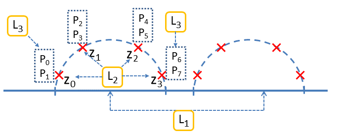
The procedure of our algorithm

Figure 3. The three levels of parallelism inherent to FEAST.

3. Proposed algorithm

In this section, we introduce our new algorithm PDESHEP, which can be seen as a hybrid algorithm, that combines the techniques of direct and iterative methods.

To reduce computational complexity, the direct methods first reduce a dense matrix $A$ to a canonical form such as tridiagonal, bidiagonal or Hessenberg, and then apply QR, DC or MRRR to compute the eigenvalue or singular value decomposition. PDESHEP also follows this approach. It first reduces a dense Hermitian matrix to its banded form via a sequence of unitary transformations. In contrast to classical direct algorithms, PDESHEP uses spectrum slicing methods to compute the eigendecomposition of the banded matrix. After obtaining the eigenpairs of the banded matrix, the eigenvectors of $A$ are computed via backtransforms. The advantage is that it gets around the SBR process, which consists of memory-bound operations and has poor scalability just as shown in Example 1 in section 4.

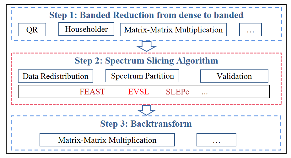
Figure 4. The structure of PDESHEP.

The procedure of PDESHEP is shown in Algorithm 2 and see also Figure 4. The structure of PDESHEP looks like a sandwich: the two outer layers remain unchanged as in the classical direct methods, but the inner kernel is replaced by an iterative method. PDESHEP is more like a framework, and we do not specify which spectrum slicing algorithm to use. Step 2 of PDESHEP can use any of the four types of spectrum slicing algorithms mentioned in section 1. In Algorithm 2, the input initial vectors $\widehat{X}_{m_{i}}^{(\ell-1)}$ are constructed from the eigenvectors of the banded matrix reduced from previous (dense) Hermitian matrix $A^{(\ell-1)}$, which may be interlaced with some random vectors when more initial vectors are required. Note that $\widehat{X}_{m_{i}}^{(\ell-1)}$ are the eigenvectors of the intermediate banded matrix instead of the original dense Hermitian matrix. The classical dense numerical linear algebra packages store matrices in 2D BCDD format such as ScaLAPACK and ELPA. The standard iterative methods usually store matrices in 1D BDD format such as FEAST (Kestyn et al., 2016) and SLEPc (Hernandez et al., 2005). We need one more data redistribution if using $X$ as the initial eigenvectors.

Input: Hermitian matrix $A^{(\ell)}$, number of eigenpairs to be computed $nev$, initial vectors $\widehat{X}_{m_{i}}^{(\ell-1)}$ for the intermediate banded matrix.

Output: The computed eigenpairs $(X,\Lambda)$, $X\in C^{n\times nev}$ and the intermediate eigenvectors $\widehat{X}_{m_{i}}^{(\ell)}$.

Step (I): Banded reduction

• Apply block Householder transformations to $A^{(\ell)}$ and reduce it to a banded matrix,

  $$D^{(\ell)}=U{A^{(\ell)}}U^{H},\quad\text{ see equation~{}\eqref{eq:densetoband}.}$$

Step (II): Spectrum slicing algorithm

• Redistribute the banded matrix to each process and store it locally in compact form.

Apply a spectrum slicing algorithm to matrix $D^{(\ell)}$ by using $\widehat{X}_{m_{i}}^{(\ell-1)}$ as the initial vectors, and compute $nev$ eigenpairs in parallel,

$$D^{(\ell)}\widehat{X}=\widehat{X}\Lambda,\quad\text{ see equation~{}\eqref{eq:bandsolver}.}$$

Redistribute the computed eigenvectors $\widehat{X}$ to 2D BCDD form $\widetilde{X}$.

Step (III): Backtransform

• Compute the eigenvectors $X$ of matrix $A^{(\ell)}$ via backtransform,

  $${X}=U^{H}\widetilde{X},\quad\text{ see equation~{}\eqref{eq:backtransform}.}$$

ALGORITHM 2 PDESHEP for sequences of Hermitian eigenvalue problems

In this work, the banded eigenvalue problem is solved by the contour integral based method implemented in FEAST (Kestyn et al., 2016). We currently focus on the Hermitian standard eigenvalue problem. For the generalized eigenvalue problem, we assume it has been reduced to the standard form. FEAST can be seen as a subspace iteration eigensolver accelerated by approximate spectral projection (Peter Tang and Polizzi, 2014), and good starting vectors $\widehat{X}_{m}$ can speed up the convergence rate. Since the input matrices are correlated in our problem, we use the eigenvectors of the previous banded intermediate matrix $D^{(\ell-1)}$ as the starting vectors for the current banded matrix $D^{(\ell)}$. The intuition is that as the SCF converges, matrices $\{A^{(\ell)}\}_{\ell\geq\eta}$ change very little, and so do the intermediate banded matrices $\{D^{(\ell)}\}_{\ell\geq\eta}$ after $\eta$ SCF iterations, where $\eta$ is an integer number. Numerical results verify this fact and show that using intermediate eigenvectors computed in the previous SCF iteration as starting vectors can significantly improve the convergence, which is usually more than $1.50$ times faster, and the results are shown in Table 3 in section 4.

The dense packages such as ScaLAPACK and ELPA store the matrices in 2D BCDD form. In contrast, iterative methods, which are usually developed for sparse matrices, use 1D block data distribution to store matrices. Since the semibandwidth of the intermediate banded matrix $D$ is small, usually $n_{bw}=64$, we store the full $D$ locally on each process. Therefore, we first need a data redistribution to obtain $D$ by collecting data from all processes, which is originally stored in 2D BCDD. The process is shown in Fig. (5(a)), and then $D$ is stored compactly as in LAPACK. Later, we need to redistribute the computed eigenvectors of the banded matrix from 1D BDD to 2D BCDD after applying the spectrum slicing algorithm. This process is shown in Fig. (5(b)), and the details of data redistribution are described in (Li et al., 2021a).

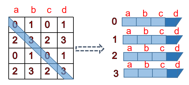
(a) The procedure of redistributing a banded matrix to 1D compact form.

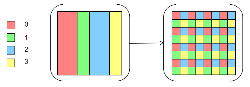
(b) Data redistribution from 1D irregular block to 2D BCDD form.

Figure 5. The data redistribution algorithms that glue direct and iterative methods.

3.1. Spectrum Partition

In spectrum slicing algorithms, the spectrum is partitioned into several slices, and the eigenvalues in each slice are computed by a group of processes. It corresponds to the first level L1 parallelism. One classical way of spectrum partition is based on Sylvester’s law of inertia, which computes the $LDL^{H}$ factorization of $A-s_{i}I$ (Golub and Loan, 1996). A more modern approach is to estimate the density of states (DOS) (Lin et al., 2016; Xi et al., 2018) of $A$, which relies on matrix-vector multiplications. The DOS has been used to partition the spectrum for the first SCF iteration in (Williams-Young et al., 2020) and EVSL (Li et al., 2019). In our problem, we could call ELPA or ScaLAPACK for the first several SCF iterations without estimating the DOS. Since the intermediate band matrix has narrow semibandwidth, $n_{bw}=64$, the cost of $LDL^{H}$ factorizations is small and the spectrum can also be partitioned by using Sylvester’s law of inertia. To reduce storage cost, we store the banded matrix in LAPACK compact form.

After the first several SCF iterations, we have prior knowledge of eigenvalues, and apply a k-means clustering method to the previous eigenvalues and partition the spectrum, just as done in (Keçeli et al., 2018; Williams-Young et al., 2020). Since the eigenvalues are stored as a one dimensional increasing array, the data structure is very simple, we propose a simplified k-means algorithm in the following subsection, which turns out to be good for the load balance problem. In this work, the aim of using k-means is to find a good partition of the spectrum, i.e., separate the clustered eigenvalues.

3.1.1. K-means Clustering

When we have a prior knowledge of the distribution of eigenvalues, we can use one clustering algorithm to divide the spectrum into different slices based on the previous computed eigenvalues. One famous clustering algorithm is the k-means algorithm (Lloyd, 1982). The goal is to group any cluster of eigenvalues into a separate slice and let the boundaries of slices not cross any cluster of eigenvalues. Figure 7 shows the boundaries of slices when partitioning $256$ eigenvalues into eight groups, where the red vertical lines mark the boundaries of slices. From it we can see that the k-means algorithm can capture the clusters of eigenvalues and separate them well. One potential problem of k-means partitioning is that different slices may be quite imbalanced, i.e., some slices may have many eigenvalues while others may have very few eigenvalues, just as shown in Figure 6, especially when partitioning into many slices. Figure 6 shows the result of partitioning the first $5000$ eigenvalues of matrix H2O from the SuiteSparse collection (Davis and Hu, 2011) into $256$ slices, where the y-axis represents the number of eigenvalues in each slice. One slice contains only two eigenvalues while another one has 40 eigenvalues. Finding the optimal clustering of eigenvalues is a difficult task. In this work, we focus more on the goodness of separation instead of the load imbalance problem. The results of Example 2 in section 4 show that the convergence rate of spectrum slicing algorithms is more sensitive to the relative gap between eigenvalues in different slices than the number of eigenvectors to be computed.

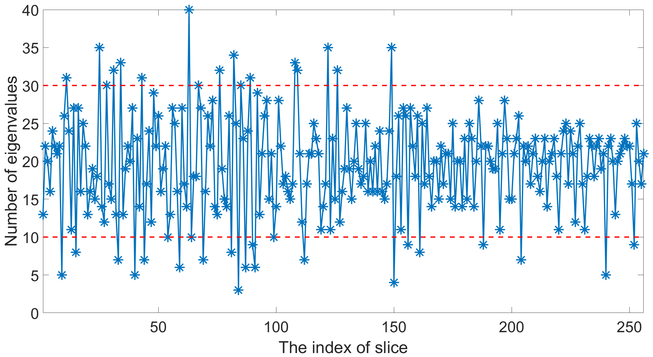
Figure 6. The number of eigenvalues of 256 slices for H2O.

A good clustering should satisfy the following objectives, see also (Keçeli et al., 2018):

1. The clustered eigenvalues (separated by less than $10^{-7}$) should be kept in the same slice;

2. The number of eigenvalues in different slices should be nearly equal;

3. The eigenvalue range with each slice should be minimized.

Objective $1$ is important for the orthogonality of computed eigenvectors, and therefore should be considered first. Objectives $2$ and $3$ concern the load imbalance problem, which is considered secondary in this paper.

The classical k-means algorithm is designed for multi-dimensional and complicated data sets, and does not exploit the simplicity in the case of a one dimensional point set. Our problem is very simple. There is a one dimensional set of points $\mathcal{C}=\{d_{1},d_{2},\cdots,d_{n}\}$, which are ordered increasingly, and we want to partition $\mathcal{C}$ into $K$ groups in the hope that each group has nearly equal number of points. We propose a simplified and fast one dimensional k-means algorithm, which has the following advantages comparing with traditional k-means algorithm.

1. This method has less computational complexity, which only requires $n+K$ floating pointing operations (flops), and $n$ is the number of points and $K$ is the number of groups. Note that classical k-means algorithm requires $(K+1)n$ flops.

2. This method usually gets a partition with smaller variance of numbers of points in all slices.

Our algorithm solves the same problem as the classical k-means method,

(16) $$J=\min_{\mu_{j}}\sum_{i=1}^{n}\sum_{j=1}^{K}\|d_{i}-\mu_{j}\|^{2},$$

where $\mu_{j},j=1,2,\cdots,K$ are the centroid of each group $G_{1},G_{2},\cdots,G_{K}.$ The whole process is shown in Algorithm 3. In our implementation, we use Euclidean norm and the centroid of group $G_{i}$ is computed as $\mu_{i}=(d_{l}+d_{r})/2$, where $d_{l}$ and $d_{r}$ are the leftmost and rightmost points in $G_{i}$, respectively. Algorithm 3 is allowed to adaptively adjust the parameter $K$ during iterations. Therefore, the return number of slices may be less than the input value $K$. When it happens, we will randomly generate $K$ centroids and run the classical k-means algorithm to generate $K$ partitions when the number of slices is given. During all our experiments, Algorithm 3 always returns the same number of slices as given by $K$.

The spectrum is partitioned by recording the number $m_{i}$ of each slice, and the boundary set $\mathcal{B}$ is updated in the next SCF iteration, $b_{i}=\frac{d_{j_{1}}+d_{j_{2}}}{2}$, where $d_{j_{1}}$ is the largest value in $G_{i}$ and $d_{j_{2}}$ is the smallest value in $G_{i+1}$. Since Algorithm 3 only costs linear time, we perform k-means clustering at every SCF iteration. But, we find it is not necessary. For the last few iteration steps of SCF before convergence, the spectrum partitions computed by Algorithm 3 are the same. When the spectrum is repartitioned, the number of eigenvalues in each slice may become different. It happens in the first few SCF iterations. When $m_{i}$ is larger than before, the previous initial vectors $\widehat{X}_{m_{i}}$ can be interlaced with some random vectors. When $m_{i}$ is smaller than before, some previous initial vectors can be removed.

We compare Algorithm 3 with two other partition approaches in section 4. One is dividing the eigenvalues equally into $K$ groups and every group has nearly the same number of eigenvalues, $nev/K$, named by Approach-1, and the boundaries of slices are computed as Algorithm 3, $b_{i}=\frac{d_{j_{1}}+d_{j_{2}}}{2}$, where $d_{j_{1}}$ is the largest value in $G_{i}$ and $d_{j_{2}}$ is the smallest value in $G_{i+1}$. Approach-1 has perfect load balance since every slice has nearly the same number of eigenvalues when used in PDESHEP. However, the boundary $b_{i}$ may be inside a cluster of eigenvalues, i.e., there are many eigenvalues near the boundary $b_{i}$, and it may introduce orthogonality problem, and slow down the convergence. The other one, Approach-2, is dividing the spectrum interval into $K$ pieces equally, which is rough. Approach-2 may have both load imbalance and orthogonality problems, and is not suggested to be used in practice.

Input: Dataset $\mathcal{C}=\{d_{1},d_{2},\cdots,d_{n}\}$ in increasing order, and the number $K$ of clusters.

Output: The boundary point set $\mathcal{B}=\{b_{0},b_{1},\cdots,b_{K}\}$, and the number set of points $\mathcal{M}=\{m_{1},m_{2},\cdots,m_{K}\}$.

1Partition $\mathcal{C}$ into $K$ groups $\{G_{i}\}_{i=1}^{K}$ such that $\left(n-\lfloor n/K\rfloor\cdotp K\right)$ groups have $\left(\lfloor n/K\rfloor+1\right)$ points and the other groups have $\lfloor n/K\rfloor$ points

2Construct $\mathcal{B}=\{b_{i}\}_{i=0}^{K}$, where $b_{i}=\frac{d_{j_{1}}+d_{j_{2}}}{2}$, where $d_{j_{1}}$ is the largest in $G_{i}$ and $d_{j_{2}}$ is the smallest in $G_{i+1}$ for $i=1,\cdots,K-1$, $b_{0}$ and $b_{K}$ are the lower and upper bounds of $\mathcal{C}$, respectively

3Let $\mathcal{B}_{0}=\{\}$

4while $(\mathcal{B}\neq\mathcal{B}_{0})$  do

       $\mathcal{B}_{0}=\mathcal{B}$

       for  $(j=1;j\leq K-1;j++)$  do

            5 $\ell=\textbf{argmin}_{d_{\ell}\in\mathcal{C}}\left\{d_{\ell}>\text{centroid}(\text{centroid}(G_{i}),\text{centroid}(G_{i+1}))\right\},$ where centroid$(\cdotp)$ is the operator of calculating the centroid

            6 $a_{i}=(d_{\ell}+d_{\ell-1})/2$

            7 update the boundary between $G_{i}$ and $G_{i+1}$, and record the number $m_{i}$ of points in $G_{i}$

            

       end for

      while  $(\exists b_{p},b_{q}\in\mathcal{B},$ s.t. $b_{p}==b_{q})$  do

            8 $\mathcal{B}=\mathcal{B}\backslash b_{q}$, $K=K-1$

            

       end while

      

end while

return $\mathcal{B}=\{b_{i}\}_{i=0}^{K},\mathcal{M}=\{m_{i}\}_{i=1}^{K}$.

ALGORITHM 3 A simplified determinate one dimensional k-means algorithm

3.2. Validation and Other Details

The contour integral based algorithm can compute all the wanted eigenvalues enclosed in a given interval. To guarantee that $nev$ eigenpairs can be computed, the lower bound $b_{0}$ and upper bound $b_{K}$ must enclose all the wanted $nev$ eigenvalues. First, the upper bound $b_{K}$ should be larger than the $nev$-th eigenvalue of the current matrix. Since we know the previous eigenvalues, $b_{K}$ can be computed by $b_{K}=(1+\alpha)d_{nev}$, where $\alpha$ is a small real number and $d_{nev}$ is the $nev$-th previous eigenvalue. Note that $b_{K}$ should not be too large. Otherwise, $[b_{0},b_{K}]$ will enclose too many eigenvalues. $b_{K}$ can be checked by computing the inertia of $(D^{(\ell)}-b_{k}I)$. If $b_{K}$ is not large enough, we iteratively enlarge it by ratio $\alpha$, $b_{K}=(1+\alpha)b_{K}$, and check it again until there are more than $nev$ eigenvalues less than $b_{K}$. Algorithm 4 illustrates process of computing the upper boundary $b_{K}$. Since LAPACK does not support $LDL^{H}$ factorization for banded symmetric matrices, we implemented a simplified version of the retraction algorithm (Kaufman, 2007), which is used to only compute the inertia without recording the matrix $L$, and the storage and computational cost are further reduced, becoming very small.

Another approach is to enlarge $b_{K}$ as $b_{K}=b_{K}+\hat{m}_{1}\delta$, where $\hat{m}_{1}$ is an integer and $\delta=d_{nev}-d_{nev-1}$, the distance between the $nev$-th and $(nev-1)$-th previous eigenvalues. When $b_{k}$ is not large enough, it will be enlarged by another $\hat{m}_{1}\delta$. Its computation is similar to the first approach. Since we are solving sequences of eigenvalue problems, the parameters $\alpha$ and $\hat{m}_{1}$ can be updated during the SCF iterations. In our implementation, we let $\alpha=\pm 10^{-3}$ and $\hat{m}_{1}=6$. For the first fewer SCF iterations, Algorithm 4 needs to iterate at most $2$–$3$ times to obtain the upper boundary point. Since $D^{(\ell)}$ is banded with small bandwidth, the computation of these inertia is very cheap.

The lower bound $b_{0}$ can be computed similarly, $b_{0}=(1+\beta)d_{1}$, and make sure $b_{0}<d_{1}$ is a lower bound. When computing the smallest few eigenvalues, the parameter $\beta$ is relatively easy to choose since any lower bound works. Similarly, $b_{0}$ can also be updated by $b_{0}=b_{0}+\hat{m}_{2}\delta_{2}$, where $\hat{m}_{2}$ is integer and $\delta_{2}=d_{1}-d_{2}$, negative. When computing interior eigenvalues, $\beta$ should be chosen carefully in case $b_{0}$ is too small to enclose too many eigenvalues in $[b_{0},b_{K}]$. Since the process is similar to Algorithm 4, it is not included.

Input: The $nev$-th previous eigenvalue $d_{nev}$ and integer $nev$, parameters $\alpha$, $\hat{m}_{1}$ and $\delta$ which equals to $d_{nev}-d_{nev-1}$, and matrix $D^{(\ell)}$.

Output: The upper boundary point ${b}_{K}$.

1Compute ${b}_{K}=d_{nev}+\max(\alpha\cdotp d_{nev},\hat{m}_{1}\delta)$

2Let $flag$=true and $it=1$

while $(flag)$  do

      3 Compute the inertia of $(D^{(\ell)}-{b}_{K}I)$, $(n_{-},n_{0},n_{+})$

       if  $(n_{-}\leq nev)$  then

            4 $flag$=false

            

       else

            5 ${b}_{K}={b}_{K}+\max(\alpha\cdotp d_{nev},\hat{m}_{1}\delta)$

            6 $it=it+1$

            

      

end while

return ${b}_{K}$.

ALGORITHM 4 Compute the upper boundary point $b_{K}$.

The spectrum is divided into $K$ slices and one process group works on one slice. Note that only the first process group needs to compute the lower boundary point $b_{0}$, and only the $K$-th process group needs to compute the upper boundary point $b_{K}$. The $i$-th process group computes the eigenvalues in the interval $(b_{i-1},b_{i})$, and every process can compute the exact number $m_{i}$ of eigenvalues in the current interval by computing the inertia of matrices $(D^{(\ell)}-b_{i-1}I)$ and $(D^{(\ell)}-b_{i}I)$. Therefore, every process group can check whether the computed eigenvalues are correct or not, and if some eigenvalues are missed, the corresponding process group should rerun FEAST by using more starting vectors.

In our problem, the value $m_{i}$ is the exact number of eigenvalues in the $i$-th slice, which is used to check the correctness of computed eigenpairs. For stability, we further enlarge the number of starting vectors in FEAST, $m_{i}^{(0)}=\max(1.3*m_{i},m_{i}+10)$. In our experiments, FEAST always computes more than $nev$ eigenvalues and no eigenvalues are missed.

4. Numerical results

All the experimental results are obtained on the Tianhe-2 supercomputer (Liao et al., 2014; Liu et al., 2016), located at Guangzhou, China. Each compute node is equipped with two $12$-core Intel Xeon E5-2692 v2 CPUs. The details of the test platform and environment of the compute nodes are shown in Table 1. For all these numerical experiments, we only used plain MPI, running $24$ MPI processes per node in principle, that is, one process per core. Our codes are written in Fortran 90 and part of our codes will be released on Github.

Table 1. The test platform and environment of one node.

Items	Values
2*CPU	Intel Xeon CPU E5-2692 v2@2.2GHz
Memory size	64GB (DDR3)
Operating System	Linux 3.10.0
Compiler	Intel ifort
Optimization	-O3 -mavx

Example 1. For the experiments in this example, we use an eigenvalue problem obtained from a DFT simulation using the FLEUR code (Blügel et al., 2017) that produces a matrix labeled NaCl, which has been used in (Winkelmann et al., 2019). This matrix is Hermitian and its size is $9273$. We use ELPA to compute partial and full eigendecomposition of this matrix, and the point is to show that step (II) has poor scalability. The codes of ELPA that we used are obtained from package ELSI v2.5.0 (Yu et al., 2020). The performance of ELPA highly depends on the parameter $n_{b}$, the block size used for storing matrices in 2D BCDD format. Many works suggest that $n_{b}=128,64,32$ are usually good choices, and smaller $n_{b}$ such as less than $16$ will degrade the performance, see (Auckenthaler et al., 2011) and (Li et al., 2021b) for more details. There are no big differences for ELPA when choosing $n_{b}=128,64$ or $32$ on Tianhe-2 supercomputer. All the performance results of ELPA are obtained by choosing $n_{b}=64$ in this paper.

The results for computing $nev=2000,5000$ and $9273$ eigenpairs are shown in Table 2 when using $64,256,1024$ and $4096$ processes. We use matrix NaCl to construct a standard eigenvalue problem, solve it by ELPA, and measure the times of step (I)-(III). From the results, we can see that

• the timings of step (II) nearly stop decreasing after $n_{p}\geq 1024$;

• step (II) takes about half of the total time, especially when $n_{p}$ is large.

Therefore, it is better to replace step (II) by a more efficient and faster solver. In this paper, we use a spectrum slicing approach for this step. The next example shows that this approach can reduce the times of step (II) by half, and our final algorithm (PDESHEP) can be more than $1.25$ times faster than ELPA.

Table 2. The execution times (in second) of each step of ELPA when choosing different $nev$.

$n_{p}$	$nev=2000$			$nev=5000$			$nev=9273$
	Step (I)	Step (II)	Step (III)	Step (I)	Step (II)	Step (III)	Step (I)	Step (II)	Step (III)
64	$7.62$	$4.49$	$1.82$	$7.67$	$8.80$	$4.49$	$7.57$	$15.10$	$8.03$
256	$3.47$	$1.96$	$0.68$	$3.44$	$3.01$	$1.50$	$3.45$	$4.78$	$2.70$
1024	$2.09$	$2.05$	$0.33$	$2.17$	$2.19$	$0.62$	$2.13$	$2.83$	$1.07$
4096	$1.85$	$2.18$	$0.32$	$1.93$	$2.03$	$0.50$	$1.92$	$2.30$	$0.54$

Example 2. In this example, we use a sequence of eigenvalue problems. It is the NaCl sequence of size $9273$, used in the previous example and in (Winkelmann et al., 2019). There are $16$ such matrices. We first use PDESHEP to compute the partial eigendecomposition of the $15$th matrix by using the eigenpairs of the $14$th and the purpose is to show that PDESHEP works for highly related eigenvalue problems. The first $256$ eigenvalues of the $14$th matrix are shown in Figure 7. Since the SCF loop is nearly converged, eigenvalues of the $15$th and $14$th matrices are quite similar and the starting vectors obtained from the $14$-th matrix are also very good approximations.

The ChASE algorithm (Winkelmann et al., 2019) computes $nev=256$ smallest eigenpairs of NaCl by using Chebyshev accelerated subspace iterations. When computing many eigenpairs, ChASE would become much slower since it does not use spectrum slicing strategy. The advantage of our algorithm is that it can compute many (even all) eigenpairs efficiently. In this example, we compute $nev=2000,5000$ and $9273$ eigenpairs for this matrix.

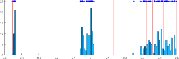
The procedure of our algorithm

Figure 7. Using k-means to clustering 256 eigenvalues of matrix NaCl into 8 groups. The red lines are the boundaries of slices, and the histogram shows the number of eigenvalues in each slice.

Let the block size $n_{b}$ be $64$, which is nearly optimal on our test platform. We first reduce the NaCl matrix to a banded Hermitian matrix with semi-bandwidth $n_{bw}=64$, and call FEAST to compute the eigenpairs in all slices simultaneously. Since step (I) and step (III) are the same as in ELPA, we mainly compare step (II) of ELPA and PDESHEP. The timing results of FEAST shown in Fig. 8 are obtained when using the eigenvectors of the banded matrix from the previous SCF iteration. If using random starting vectors, FEAST would require more time as illustrated in Table 3. From the results in Table 3, we can see that using the previous eigenvectors as starting vectors can be more than four times faster than using random starting vectors when using $4096$ processes. The results show that using previous eigenvectors as initial vectors provide a significant benefit when the eigenvalue problems are highly correlated. PDESHEP is suggested to be used for the last few SCF iterations before convergence.

Table 3. The times (in second) of FEAST with and without initial vectors when applying on the $15$-th matrix.

$n_{p}$	$nev=2000$		$nev=5000$		$nev=9273$
	With	Without	With	Without	With	Without
64	$3.75$	$5.43$	$5.86$	$8.74$	$11.70$	$18.51$
256	$1.17$	$1.96$	$2.10$	$3.27$	$3.64$	$5.15$
1024	$0.60$	$0.86$	$1.61$	$1.99$	$1.42$	$2.24$
4096	$0.87$	$3.14$	$0.62$	$2.90$	$0.71$	$2.86$

When comparing with step (II) of ELPA, we add the time of FEAST with the time spent in data redistributions. The speedups over Stage II of ELPA are shown in Fig. 8(a) when using different processes ($64,256,1024,4096$) to compute $2000,5000$ or $9273$ eigenpairs. The speedup can be up to $2\times$ when using $4096$ processes. The total speedups of PDESHEP over ELPA are shown in Fig. 8(b). PDESHEP can be more than 20% faster than ELPA when computing full or partial eigendecomposition and using $4096$ processes.

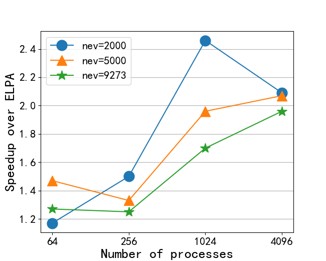
(a) The speedup over ELPA for Stage II.

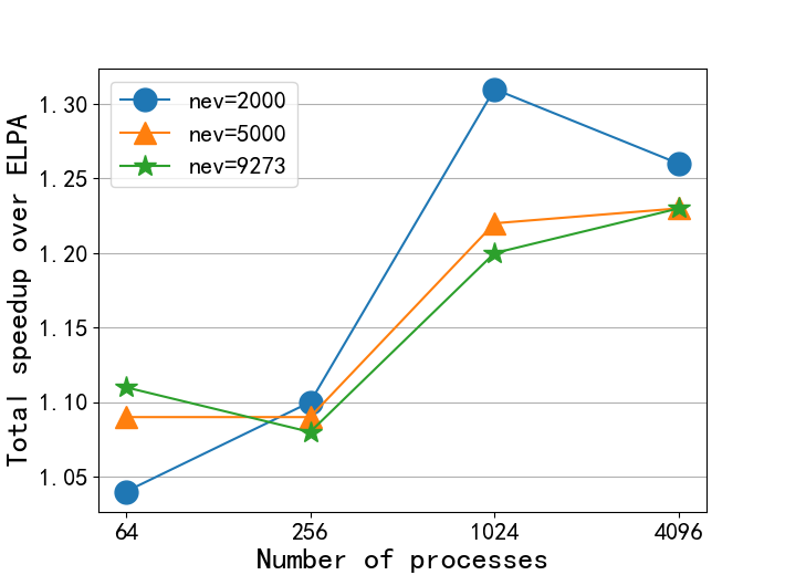
(b) The total speedup of PDESHEP over ELPA.

Figure 8. The speedup of PDESHEP over ELPA.

During the first few SCF iterations, the matrices can be quite different and so do the eigenvalues and eigenvectors. We now apply PDESHEP on a matrix on the early stages of SCF iterations and compare PDESHEP with ELPA. We choose the $10$-th NaCl matrix and use the same parameter $\epsilon=10^{-11}$. We first compute the eigendecomposition of the $10$-th NaCl matrix and using its eigenvalues to partition the spectrum of the $11$-th matrix. Then, we use eigenvectors of the $10$-th matrix as initial vectors of FEAST. We see that the ‘good‘ estimated initial vectors do help the convergence of FEAST but they are not as significant as that obtained on the $15$-th matrix. The results are shown in Table 4, where the column With shows the times (in second) cost by step (II) of FEAST when the initial vectors are constructed from the eigenvectors of the $5$-th matrix; the column Without shows the times when using random vectors as initial vectors; the column ELPA shows the times cost by step (II) of ELPA. For this matrix, we use at most $1024$ processes. From the results, we can see that PDESHEP can still be faster than ELPA for the $11$-th matrix.

Table 4. The times (in second) of FEAST with and without initial vectors when applying on the $11$-th matrix with $\epsilon=10^{-11}$.

$n_{p}$	$nev=2000$			$nev=5000$			$nev=9273$
	With	Without	ELPA	With	Without	ELPA	With	Without	ELPA
64	$3.22$	$4.12$	$4.49$	$6.91$	$10.25$	$8.80$	$14.58$	$18.97$	$15.10$
256	$1.57$	$2.16$	$1.96$	$2.80$	$3.72$	$3.01$	$4.66$	$5.75$	$4.78$
1024	$1.19$	$1.84$	$2.05$	$1.74$	$2.24$	$2.19$	$2.56$	$3.45$	$2.83$

For the matrices appeared at the even earlier stages of SCF, for example the $5$-th matrix, the ’good’ estimated initial vectors and eigenvalues help very little. FEAST may cost more than step (II) of ELPA when computing the eigenpairs accurately with $\epsilon=10^{-11}$. However, at the early stages of SCF iterations, the eigenvalue problems only need to be solved approximately. Therefore, we let $\epsilon=10^{-9}$ and find that step (II) of PDESHEP is also faster than that of ELPA, and the results are shown in Table 5 for the $6$-th matrix with $\epsilon=10^{-9}$.

Table 5. The times (in second) of step (II) for FEAST with and without initial vectors when applying on the $6$-th matrix with $\epsilon=10^{-9}$.

$n_{p}$	$nev=2000$			$nev=5000$			$nev=9273$
	With	Without	ELPA	With	Without	ELPA	With	Without	ELPA
64	$3.35$	$4.38$	$4.49$	$7.22$	$10.18$	$8.80$	$13.12$	$18.66$	$15.10$
256	$1.30$	$1.76$	$1.96$	$2.84$	$3.44$	$3.01$	$4.16$	$5.73$	$4.78$
1024	$1.18$	$1.91$	$2.05$	$1.88$	$2.84$	$2.19$	$2.46$	$3.57$	$2.83$

In this paper, the orthogonality is measured as

(17) $$\mathrm{Orth}=\frac{\|X^{H}X-I\|_{\max}}{n},$$

where $n$ is the dimension of the matrix, $X$ is the computed eigenvector matrix and $I$ is the identity matrix of size $nev$. The orthogonality of computed eigenvectors is shown in Fig. 9, being about or less than $10^{-13}$ in all cases, an acceptable value for most material simulations. Though the orthogonality of eigenvectors computed by PDESHEP is not as accurate as those obtained by direct methods, which is usually around the machine precision, it should be accurate enough for the SCF iterations, The computed residuals of eigenpairs are all less than $10^{-11}$ since the residual tolerance of FEAST is chosen to be $\epsilon=10^{-11}$ in this paper. In the previous work (Aktulga et al., 2014), the residual tolerance was $10^{-10}$, a little larger than that used in this paper.

Since ChASE does not implement the spectrum slicing techniques, it is suggested to compute less than $10$% eigenpairs of matrix (Aktulga et al., 2014). We use ChASE to compute the first $1000$ eigenpairs of the $15$-th NaCl matrix, and the orthogonality of computed eigenvector by ChASE is around $10^{-18}$ which is more accurate than those computed by PDESHEP, but ChASE costs much more time than PDESHEP. If we let $\epsilon=10^{-12}$, the orthogonality of computed eigenvectors by PDESHEP are also improved, around $10^{-16}$, when using $64$, $256$ and $512$ MPI processes. The results are shown in Table 6. The convergence of FEAST depends on the parameter $\epsilon$, and we find it may take FEAST a lot of iterations to converge if $\epsilon<10^{-13}$.

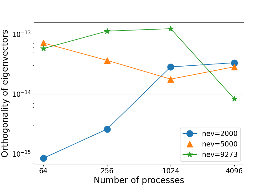
Figure 9. The orthogonality of computed eigenvectors of matrix NaCl.

Table 6. The orthogonality of eigenvectors computed by ChASE and PDESHEP for the $15$-th NaCl matrix.

Method	$n_{p}=64$	$n_{p}=256$	$n_{p}=512$
PDESHEP	$9.49e$-$16$	$9.48e$-$16$	$9.40e$-$16$
ChASE	$2.22e$-$18$	$1.41e$-$18$	$1.84e$-$18$

The results of this example show that PDESHEP can compute both partial and full eigendecomposition efficiently and the computed eigenvectors are orthogonal with acceptable accuracy when the slices are constructed carefully. From our experimental results, we claim that the k-means based spectrum partition strategy (Algorithm 3) is helpful for the orthogonality of computed eigenvectors. We compare Algorithm 3 with two other partition approaches: Approach-1 and Approach-2, and Algorithm 3 performs the best.

Example 3. In this example, we use some relatively large matrices to test our algorithm. The first class is AuAg with dimension $n=13,379$, which originates from simulations using FLAPW (Jansen and Freeman, 1984) and has been used in (Winkelmann et al., 2019). They have different spectral distribution compared to the NaCl dataset. There are $25$ such matrices, and we compute the eigendecomposition of the $24$th matrix by using the information from the $23$th matrix.

The other two matrices are from the SuiteSparse collection (Davis and Hu, 2011). One is Si5H12 with $n=19,896$ and $nnz=379,247$, and the other is the H2O matrix with $n=67,024$ and $nnz=2,216,736$, which are both real symmetric and sparse. Since there is only one such matrix for each type, we construct another two matrices by adding a small random symmetric perturbation to the nonzero entries of these matrices such that they have the same structure and similar eigenvalues. The nonzero entry $a_{i,j}$ is perturbed as

(18) $$a_{i,j}=a_{i,j}(1+\tau\eta_{i,j}),$$

where $\tau=10^{-4}$ and $\eta_{i,j}$ is a random real number in the interval $[0,1]$. Note that the contour integral based algorithms always operate with complex arithmetic. Therefore, FEAST may require more flops than other iterative methods for real matrices.

In this example, we compute the first $5000$ smallest eigenpairs and use $256,1024$ and $4096$ processes, respectively. The results of ELPA are shown in Table 7. For these experiments, the convergence residual tolerance is also $\epsilon=10^{-11}$, and the dimension of the subspace is $m_{i}^{(0)}=\max(1.3\times m_{i},m_{i}+10)$, where $m_{i}$ is the estimated number of eigenvalues in the current slice. We note that $m_{i}^{(0)}$ can affect the performance considerably. When $m_{i}^{(0)}$ is small, it makes the linear equations with fewer right-hand sides much easier to solve. When $m_{i}^{(0)}$ is too small, it may make FEAST not converge. There is a trade-off between speed and robustness.

Table 7. The execution times (in second) of each step of ELPA for large matrices.

$n_{p}$	AuAg			Si5H12			H2O
	Step (I)	Step (II)	Step (III)	Step (I)	Step (II)	Step (III)	Step (I)	Step (II)	Step (III)
256	$8.19$	$5.47$	$2.87$	$6.84$	$5.82$	$2.08$	$17.41$	$67.03$	$18.87$
1024	$4.01$	$3.56$	$1.13$	$4.13$	$4.45$	$1.21$	$64.34$	$24.72$	$9.70$
4096	$3.29$	$4.17$	$0.76$	$3.79$	$4.14$	$1.28$	$27.45$	$17.53$	$5.57$

The speedups of FEAST over step (II) of ELPA are shown in Fig. 10(a). The results in Fig 10(a) show that it is difficult to predict the speedup of spectrum slicing algorithms over Stage II of ELPA, that is because the partition of the spectrum may affect the performance of spectrum slicing algorithms. It is also very hard to know how many slices to partition is best, which depends on the distribution of eigenvalues and the used spectrum slicing algorithm. Figure 6 shows the number of eigenvalues of the $256$ slices for H2O when using $4096$ processes. It is not well balanced, and most slices have eigenvalues between $10$ and $30$, but one slice only has $2$ eigenvalues and one slice has $40$ eigenvalues. Comparing with load imbalance problem, we find that good separation of eigenvalues may be more important. If one boundary is inside a cluster of eigenvalues, it may introduce convergence and orthogonality problems. We use our simplified k-means algorithm to partition the spectrum, and the load balance problem is also taken into account. The total speedups of PDESHEP over ELPA are shown in Fig. 10(b), which are always larger than $1.20$ and up to $1.49$ when using $4096$ processes. The wall times of FEAST used to compute the second step, step (II), are shown in Table 8.

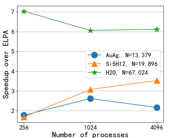
(a) The speedup over ELPA for Stage II.

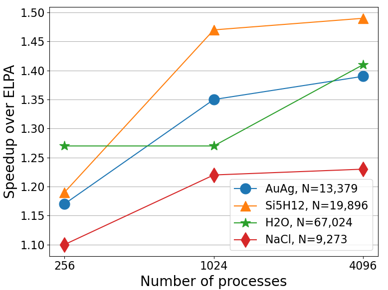
(b) The total speedup of PDESHEP over ELPA.

Figure 10. The speedup of PDESHEP over ELPA for large matrices.

Table 8. The execution times of step (II) in second of PDESEHP for large matrices.

$n_{p}$	AuAg	Si5H12	H2O
256	$3.08$	$3.44$	$9.53$
1024	$1.36$	$1.44$	$4.07$
4096	$1.92$	$1.17$	$2.86$

5. Conclusions and future works

In this paper, we propose a new framework for computing partial or full eigendecomposition of dense Hermitian or real symmetric matrices, which can be easily extended to generalized eigenvalue problems. This new framework is denoted by PDESHEP, which combines the classical direct methods with spectrum slicing algorithms. In this work, we combine ELPA (Auckenthaler et al., 2011) with FEAST (Kestyn et al., 2016). PDESHEP can also be combined with other spectrum slicing algorithms such as those implemented in SLEPc (Campos and Roman, 2012) or EVSL (Li et al., 2019). This will be a topic for future work.

In PDESHEP, a dense matrix is first reduced to a banded form and then spectrum slicing algorithms are used to compute its partial eigendecomposition instead of further reducing it to tridiagonal form. Therefore, the symmetric bandwidth reduction (SBR) process is avoided, which consists of memory-bounded operations. For self-consistent field (SCF) eigenvalue problems which are correlated, PDESHEP can be about $1.25$ times faster than ELPA. Numerical results are obtained on Tianhe-2 supercomputer and up to $4096$ processes are used. The tested matrices include dense Hermitian matrices from real applications, and large real symmetric sparse matrices downloaded from the SuiteSparse collection (Davis and Hu, 2011). Another future work is to incorporate PDESHEP into ELSI (Yu et al., 2020) or some electronic-structure calculation packages such as QE (Giannozzi et al., 2009) to do some real simulations.

- (1)
- Aktulga et al. (2014) Hasan Metin Aktulga, Lin Lin, Christopher Haine, Esmond G Ng, and Chao Yang. 2014. Parallel eigenvalue calculation based on multiple shift–invert Lanczos and contour integral based spectral projection method. Parallel Comput. 40, 7 (2014), 195–212.
- Arbenz (1992) P. Arbenz. 1992. Divide-and-Conquer algorithms for the bandsymmetric eigenvalue problem. Parallel Comput. 18 (1992), 1105–1128.
- Auckenthaler et al. (2011) T. Auckenthaler, V. Blum, H. J. Bungartz, T. Huckle, R. Johanni, L. Krämer, B. Lang, H. Lederer, and P. R. Willems. 2011. Parallel solution of partial symmetric eigenvalue problems from electronic structure calculations. Parallel Comput. 37, 12 (2011), 783–794.
- Bai et al. (2000) Z. Bai, J. Demmel, J. Dongarra, A. Ruhe, and H. van der Vorst. 2000. Templates for the solution of algebraic eigenvalue problems A practical Guide. Society for Industrial and Applied Mathematics, Philadelphia, PA.
- Banerjee et al. (2016) Amartya S Banerjee, Lin Lin, Wei Hu, Chao Yang, and John E Pask. 2016. Chebyshev polynomial filtered subspace iteration in the discontinuous Galerkin method for large-scale electronic structure calculations. The Journal of chemical physics 145, 15 (2016), 154101.
- Bischof et al. (1994) C. Bischof, B. Lang, and X. Sun. 1994. Parallel tridiagonalization through two-step band reduction. In Proceedings of the Scalable High-Performance Computing Conference. IEEE Computer Society Press, Los Alamitos, CA, 23–27.
- Bischof et al. (2000) C. H. Bischof, B. Lang, and X. B. Sun. 2000. Algorithm 807: The SBR toolbox-software for successive band reduction. ACM Trans. Math. Softw. 26, 4 (2000), 602–616.
- Blackford et al. (1997) J. S. Blackford, J. Choi, A. Cleary, E. D’Azevedo, J. Demmel, I. Dhillon, J. Dongarra, S. Hammarling, G. Henry, A. Petitet, K. Stanley, D. Walker, and R. C. Whaley. 1997. ScaLAPACK Users’ Guide. Society for Industrial and Applied Mathematics, Philadelphia, PA.
- Blügel et al. (2017) Stefan Blügel, Gustav Bihlmayer, and Daniel Wortmann. 2017. The FLEUR Code. Website: http://www.flapw.de.
- Campos and Roman (2012) Carmen Campos and Jose E Roman. 2012. Strategies for spectrum slicing based on restarted Lanczos methods. Numerical Algorithms 60, 2 (2012), 279–295.
- Cuppen (1981) J. J. M. Cuppen. 1981. A divide and conquer method for the symmetric tridiagonal eigenproblem. Numer. Math. 36 (1981), 177–195.
- Davis and Hu (2011) Timothy A Davis and Yifan Hu. 2011. The University of Florida sparse matrix collection. ACM Transactions on Mathematical Software (TOMS) 38, 1 (2011), 1–25.
- Dhillon (1997) I. S. Dhillon. 1997. A New Algorithm for the Symmetric Tridiagonal Eigenvalue/Eigenvector Problem. Ph.D. Dissertation. Computer Science Division, University of California, Berkeley, California.
- Dhillon et al. (2006) I. S. Dhillon, B. N. Parlett, and C. Vömel. 2006. The design and implementation of the MRRR algorithm. ACM Trans. Math. Softw. 32, 4 (2006), 533–560.
- Francis (1962) John GF Francis. 1962. The QR transformation–part 2. Comput. J. 4, 4 (1962), 332–345.
- Gansterer et al. (2002) W. N. Gansterer, R. C. Ward, and R. P. Muller. 2002. An extension of the divide-and-conquer method for a class of symmetric block-tridiagonal eigenproblems. ACM Trans. Math. Softw. 28, 1 (2002), 45–58.
- Giannozzi et al. (2009) Paolo Giannozzi, Stefano Baroni, Nicola Bonini, Matteo Calandra, Roberto Car, Carlo Cavazzoni, Davide Ceresoli, Guido L Chiarotti, Matteo Cococcioni, Ismaila Dabo, et al. 2009. QUANTUM ESPRESSO: a modular and open-source software project for quantum simulations of materials. Journal of physics: Condensed matter 21, 39 (2009), 395502.
- Golub and Loan (1996) G. H. Golub and C. F. Van Loan. 1996. Matrix Computations (3rd ed.). The Johns Hopkins University Press, Baltimore, MD.
- Grimes et al. (1994) Roger G Grimes, John G Lewis, and Horst D Simon. 1994. A shifted block Lanczos algorithm for solving sparse symmetric generalized eigenproblems. SIAM J. Matrix Anal. Appl. 15, 1 (1994), 228–272.
- Gu and Eisenstat (1995) M. Gu and S. C. Eisenstat. 1995. A divide-and-conquer algorithm for the symmetric tridiagonal eigenproblem. SIAM J. Matrix Anal. Appl. 16 (1995), 172–191.
- Guttel et al. (2015) Stefan Guttel, Eric Polizzi, Ping Tak Peter Tang, and Gautier Viaud. 2015. Zolotarev quadrature rules and load balancing for the FEAST eigensolver. SIAM Journal on Scientific Computing 37, 4 (2015), A2100–A2122.
- Haidar et al. (2012) A. Haidar, H. Ltaief, and J. Dongarra. 2012. Toward a high performance tile divide and conquer algorithm for the dense symmetric eigenvalue problem. SIAM J. Sci. Comput. 34, 6 (2012), C249–C274.
- Hernandez et al. (2005) V. Hernandez, J. E. Roman, and V. Vidal. 2005. SLEPc: A Scalable and Flexible Toolkit for the solution of eigenvalue problems. ACM Trans. Math. Softw. 31, 3 (2005), 351–362.
- Imamura et al. (2011) T. Imamura, S. Yamada, and M. Yoshida. 2011. Development of a high-performance eigensolver on a peta-scale next-generation supercomputer system. Prog. Nucl. Sci. Technol. 2 (2011), 643–650.
- Jansen and Freeman (1984) HJF Jansen and Arthur J Freeman. 1984. Total-energy full-potential linearized augmented-plane-wave method for bulk solids: Electronic and structural properties of tungsten. Physical Review B 30, 2 (1984), 561.
- Kaufman (2007) Linda Kaufman. 2007. The retraction algorithm for factoring banded symmetric matrices. Numerical Linear Algebra with Applications 14, 3 (2007), 237–254.
- Keçeli et al. (2018) Murat Keçeli, Fabiano Corsetti, Carmen Campos, Jose E Roman, Hong Zhang, Álvaro Vázquez-Mayagoitia, Peter Zapol, and Albert F Wagner. 2018. SIESTA-SIPs: Massively parallel spectrum-slicing eigensolver for an ab initio molecular dynamics package. Journal of Computational Chemistry 39, 22 (2018), 1806–1814.
- Keçeli et al. (2016) Murat Keçeli, Hong Zhang, Peter Zapol, David A Dixon, and Albert F Wagner. 2016. Shift-and-invert parallel spectral transformation eigensolver: Massively parallel performance for density-functional based tight-binding. Journal of computational chemistry 37, 4 (2016), 448–459.
- Kestyn et al. (2016) James Kestyn, Vasileios Kalantzis, Eric Polizzi, and Yousef Saad. 2016. PFEAST: a high performance sparse eigenvalue solver using distributed-memory linear solvers. In SC’16: Proceedings of the International Conference for High Performance Computing, Networking, Storage and Analysis. IEEE, 178–189.
- Knyazev (2001) Andrew V Knyazev. 2001. Toward the optimal preconditioned eigensolver: Locally optimal block preconditioned conjugate gradient method. SIAM journal on scientific computing 23, 2 (2001), 517–541.
- Kohn (1999) Walter Kohn. 1999. Nobel Lecture: Electronic structure of matter—wave functions and density functionals. Reviews of Modern Physics 71, 5 (1999), 1253.
- Lehoucq et al. (1998) Richard B Lehoucq, Danny C Sorensen, and Chao Yang. 1998. ARPACK users’ guide: solution of large-scale eigenvalue problems with implicitly restarted Arnoldi methods. SIAM.
- Li et al. (2019) Ruipeng Li, Yuanzhe Xi, Lucas Erlandson, and Yousef Saad. 2019. The eigenvalues slicing library (EVSL): Algorithms, implementation, and software. SIAM Journal on Scientific Computing 41, 4 (2019), C393–C415.
- Li et al. (2016) Ruipeng Li, Yuanzhe Xi, Eugene Vecharynski, Chao Yang, and Yousef Saad. 2016. A Thick-Restart Lanczos algorithm with polynomial filtering for Hermitian eigenvalue problems. SIAM Journal on Scientific Computing 38, 4 (2016), A2512–A2534.
- Li et al. (2021a) Shengguo Li, Hao Jiang, Dezun Dong, Chun Huang, Jie Liu, Xia Liao, and Xuguang Chen. 2021a. Efficient data redistribution algorithms from irregular to block cyclic data distribution. submitted to IEEE Transactions on parallel and distributed systems (Minor revision).
- Li et al. (2021b) Shengguo Li, Xia Liao, Yutong Lu, Jose E. Roman, and Xiaoqiang Yue. 2021b. A parallel structured banded DC algorithm for symmetric eigenvalue problems. Submitted to CCF Transactions on High Performance Computing (2021).
- Liao et al. (2016) X. Liao, S. Li, L. Cheng, and M. Gu. 2016. An improved divide-and-conquer algorithm for the banded matrices with narrow bandwidths. Comput. Math. Appl. 71 (2016), 1933–1943.
- Liao et al. (2014) X. Liao, L. Xiao, C. Yang, and Y. Lu. 2014. MilkyWay-2 supercomputer: system and application. Front. Comput. Sci. 8, 3 (2014), 345–356.
- Lin et al. (2016) Lin Lin, Yousef Saad, and Chao Yang. 2016. Approximating spectral densities of large matrices. SIAM review 58, 1 (2016), 34–65.
- Liu et al. (2016) Y. Liu, C. Yang, F. Liu, X. Zhang, Y. Lu, Y. Du, C. Yang, M. Xie, and X. Liao. 2016. 623 Tflop/s HPCG run on Tianhe-2: Leveraging millions of hybrid cores. International Journal of High Performace Computing Applications 30, 1 (2016), 39–54.
- Lloyd (1982) Stuart Lloyd. 1982. Least squares quantization in PCM. IEEE transactions on information theory 28, 2 (1982), 129–137.
- Marek et al. (2014) A. Marek, V. Blum, R. Johanni, V. Havu, B. Lang, T. Auckenthaler, A. Heinecke, H. Bungartz, and H. Lederer. 2014. The ELPA library: scalable parallel eigenvalue solutions for electronic structure theory and computational science. J. Phys.: Condens. Matter 26 (2014), 1–15.
- Parlett (1998) B. N. Parlett. 1998. The symmetric eigenvalue problem. SIAM, Philadelphia.
- Peter Tang and Polizzi (2014) Ping Tak Peter Tang and Eric Polizzi. 2014. FEAST as a subspace iteration eigensolver accelerated by approximate spectral projection. SIAM J. Matrix Anal. Appl. 35, 2 (2014), 354–390.
- Petschow et al. (2013) M. Petschow, E. Peise, and P. Bientinesi. 2013. High-performance solvers for dense Hermitian eigenproblems. SIAM J. Numer. Anal. 35 (2013), C1–C22.
- Polizzi (2009) Eric Polizzi. 2009. Density-matrix-based algorithm for solving eigenvalue problems. Physical Review B 79, 11 (2009), 115112.
- Polizzi and Sameh (2007) Eric Polizzi and Ahmed Sameh. 2007. SPIKE: A parallel environment for solving banded linear systems. Computers & Fluids 36, 1 (2007), 113–120.
- Poulson et al. (2013) J. Poulson, B. Marker, R. A. van de Geijn, J. R. Hammond, and N. A. Romero. 2013. Elemental: A new framework for distributed memory dense matrix computations. ACM Trans. Math. Software 39, 2 (2013), 13:1–13:24.
- Saad (2011) Y. Saad. 2011. Numerical Methods for Large eigenvalue problems. SIAM, Philadelphia, PA.
- Sakurai and Sugiura (2003) T. Sakurai and H. Sugiura. 2003. A projection method for generalized eigenvalue problems using numerical integration. J. Comput. Appl. Math. 159 (2003), 119–128.
- Sakurai and Tadano (2007) Tetsuya Sakurai and Hiroto Tadano. 2007. CIRR: a Rayleigh-Ritz type method with contour integral for generalized eigenvalue problems. Hokkaido Mathematical Journal 36, 4 (2007), 745–757.
- Salas et al. (2015) Pablo Salas, Luc Giraud, Yousef Saad, and Stéphane Moreau. 2015. Spectral recycling strategies for the solution of nonlinear eigenproblems in thermoacoustics. Numerical Linear Algebra with Applications 22, 6 (2015), 1039–1058.
- Silver and Röder (1994) RN Silver and H Röder. 1994. Densities of states of mega-dimensional Hamiltonian matrices. International Journal of Modern Physics C 5, 04 (1994), 735–753.
- Sylvester (1852) James Joseph Sylvester. 1852. XIX. A demonstration of the theorem that every homogeneous quadratic polynomial is reducible by real orthogonal substitutions to the form of a sum of positive and negative squares. The London, Edinburgh, and Dublin Philosophical Magazine and Journal of Science 4, 23 (1852), 138–142.
- Tisseur and Dongarra (1999) F. Tisseur and J. Dongarra. 1999. A parallel divide and conquer algorithm for the symmetric eigenvalue problem on distributed memory architectures. SIAM J. Sci. Comput. 20, 6 (1999), 2223–2236.
- Wang (1994) Lin-Wang Wang. 1994. Calculating the density of states and optical-absorption spectra of large quantum systems by the plane-wave moments method. Physical Review B 49, 15 (1994), 10154.
- Willems and Lang (2013) Paul R Willems and Bruno Lang. 2013. A Framework for the Algorithm: Theory and Implementation. SIAM Journal on Scientific Computing 35, 2 (2013), A740–A766.
- Williams-Young et al. (2020) David B Williams-Young, Paul G Beckman, and Chao Yang. 2020. A Shift Selection Strategy for Parallel Shift-Invert Spectrum Slicing in Symmetric Self-Consistent Eigenvalue Computation. ACM Transactions on Mathematical Software (TOMS) 46, 4 (2020), 1–31.
- Winkelmann et al. (2019) Jan Winkelmann, Paul Springer, and Edoardo Di Napoli. 2019. ChASE: Chebyshev Accelerated Subspace iteration Eigensolver for sequences of Hermitian eigenvalue problems. ACM Transactions on Mathematical Software (TOMS) 45, 2 (2019), 1–34.
- Xi et al. (2018) Yuanzhe Xi, Ruipeng Li, and Yousef Saad. 2018. Fast computation of spectral densities for generalized eigenvalue problems. SIAM Journal on Scientific Computing 40, 4 (2018), A2749–A2773.
- Yu et al. (2020) Victor Wen-zhe Yu, Carmen Campos, William Dawson, Alberto García, Ville Havu, Ben Hourahine, William P Huhn, Mathias Jacquelin, Weile Jia, Murat Keçeli, et al. 2020. ELSI–An open infrastructure for electronic structure solvers. Computer Physics Communications 256 (2020), 107459.
- Zhang et al. (2007) Hong Zhang, Barry Smith, Michael Sternberg, and Peter Zapol. 2007. SIPs: Shift-and-invert parallel spectral transformations. ACM Transactions on Mathematical Software (TOMS) 33, 2 (2007), 1–19.