Mixed Information Flow for Cross-domain Sequential Recommendations

Abstract.

Cross-domain sequential recommendation is the task of predict the next item that the user is most likely to interact with based on past sequential behavior from multiple domains. One of the key challenges in cross-domain sequential recommendation is to grasp and transfer the flow of information from multiple domains so as to promote recommendations in all domains. Previous studies have investigated the flow of behavioral information by exploring the connection between items from different domains. The flow of knowledge (i.e., the connection between knowledge from different domains) has so far been neglected. In this paper, we propose a mixed information flow network for cross-domain sequential recommendation to consider both the flow of behavioral information and the flow of knowledge by incorporating a behavior transfer unit and a knowledge transfer unit. The proposed mixed information flow network is able to decide when cross-domain information should be used and, if so, which cross-domain information should be used to enrich the sequence representation according to users’ current preferences. Extensive experiments conducted on four e-commerce datasets demonstrate that mixed information flow network is able to further improve recommendation performance in different domains by modeling mixed information flow.

1. Introduction

Sequential recommendation (SR) aims to predict the next item that the user is most likely to interact with based on her/his past sequential behavior (e.g., clicks on items) (Quadrana et al., 2017). Recently, cross-domain sequential recommendation (CDSR) has emerged as a way to promote recommendation performance by leveraging and combining information from different domains (Ma et al., 2019a). Users usually have related preferences in different domains, such as finding a movie with a certain style or looking for a book written by a well-known author, as illustrated in Figure 1. One of the key challenges in CDSR is to capture and transfer useful information about related preferences across different domains.

Figure 1. Illustration of a connection between a user’s behavioral information across domains via a knowledge graph. Lines in different colors represent different connections.

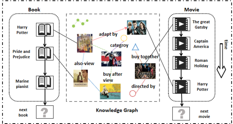
Zhuang et al. (2018) and Ma et al. (2019a) have shown that behavioral information across domains is helpful for improving recommendation performance. However, behavioral information by itself can only support the use of cross-domain connections in a limited manner. Behavioral information may be insufficient for a model to capture fine-grained connections between item attributes or features. For example, as illustrated in Figure 1, assume there is a user who has read Harry Potter (the book) and watched Captain America (the movie). If there is no external knowledge to indicate that both items belong to the category of “fantasy,” it is difficult for the model to capture this connection based solely on the user’s behavior from both domains. We hypothesize that enabling a flow of knowledge across different domains is able to alleviate this issue. As a result, for a user who has read the book The Great Gatsby, we then can recommend her/him a movie having the same name or movies featuring the same category of “tragic love,” such as Atonement, Waterloo Bridge, and so on, when she/he logs on to the movie recommendation system.

There is a growing body of work aimed at improving recommendation performance by using knowledge (Ren et al., 2020b; Lin et al., 2019). Of particular relevance to us is work that has proposed to incorporate knowledge and combine it with behavioral information for sequential recommendation (SR) (see, e.g., Huang et al., 2018; Wu et al., 2019; Huang et al., 2019). However, this work targets a single domain recommendation scenario. The situation is dramatically different in cross-domain scenarios where it is necessary to distinguish information from different domains and effectively link them. We need to select behavioral and knowledge related to users’ current preference, and determine when and what to use in order to learn a better sequence representation.

To address the issue of using behavioral information and knowledge across domains, we propose a mixed information flow network (MIFN) to consider mixed information flow across domains, i.e., the flow of behavioral information as well as the flow of knowledge. The former is based on user’s behavior, which captures the temporal connection between the items they have interacted with, while the latter takes cross-domain knowledge as a bridge to connect different domains to obtain better cross-domain sequence representations. First, we employ a behavior transfer unit (BTU) to grasp useful information from the flow of behavioral information, which can extract information related to the user’s preference and then transfer it to another domain at the level of user behavior level. Then, we propose a knowledge transfer unit (KTU) that is guided by the user’s preference to model the connection between items from different domains; we introduce a cross-domain graph convolutional mechanism to distinguish items in the knowledge graph (KG) and grasp useful information for fusion at the knowledge level. Finally, we generate recommendations based on the fusion of the two types of information. During learning, mixed information flow network (MIFN) is jointly trained on multiple domains in an end-to-end back-propagation training paradigm. Experiments on the Amazon datasets show that MIFN outperforms state-of-the-art methods in terms of MRR and Recall.

To sum up, the contributions of this work are as follows:

• We propose a mixed information flow framework, MIFN, for CDSR, which consists of a behavior transfer unit and a knowledge transfer unit to simultaneously model the flow of behavioral information and of knowledge across domains.

• We devise a cross-domain graph convolutional mechanism to disseminate item information in the KG, which leads to the better up-to-date item representation.

• We conduct experiments to demonstrate that MIFN is able to improve recommendation performance in different domains by modeling mixed information flow.

2. Related work

In this section, we briefly introduce related work from the following categories: (1) sequential recommendation, (2) cross-domain recommendation, and (3) knowledge-aware recommendation.

2.1. Sequential recommendations

Early work on recommender systems typically use collaborative filtering (CF) to generate recommendations (Hu et al., 2018a) according to users’ preferences reflected in similar items such as K-Nearest neighbors (KNN) or matrix factorization (MF) algorithms. Such methods do not consider sequential aspects. More recently, however, SR and next-basket recommendation have witnessed rapid developments.

Before the widespread application of deep learning, Markov chainss (Zimdars et al., 2001; Rendle et al., 2010; Chen et al., 2012; He and McAuley, 2016) and Markov decision processs (Shani et al., 2005; Wu et al., 2013) have been used to predict users’ next action given information about their past behavior (Wang et al., 2015; Yap et al., 2012). All these methods take into account the sequential characteristics. However, there are considerable challenges with the size of the state when considering the entire sequence (Quadrana et al., 2018).

RNN have been introduced to SR to handle variable-length sequential data. Hidasi et al. (2016a) are the first to leverage recurrent neural networks for SR. They utilize session-parallel mini-batch training and employ ranking-based loss functions to train the model. Then, Tan et al. (2016) propose two techniques to improve the performance, i.e., data augmentation and a method to account for shifts in the input data distribution. Li et al. (2017) incorporate an attention mechanism into the encoder to capture the users’ main preference in the current sequence. Ren et al. (2019) point out the repeat consumption in SR, where the same item is re-consumed repeatedly over time. Quadrana et al. (2017) propose a hierarchical RNN model that can relay and evolve latent hidden states of the RNNs across user sequences. Donkers et al. (2017) explicitly model user information in a gated architecture with extra input layers for gated recurrent unit (GRU). Memory enhanced RNN has been well studied for SR recently. Chen et al. (2018) introduce a memory mechanism to SR and design a memory-augmented neural network integrated with the insights of CF. Wang et al. (2019c) propose two parallel memory modules: one to model a user’s own information in the current sequence and the other to exploit collaborative information in neighborhood sequences. Wu et al. (2019) argue that prior work on conventional sequential methods neglects complex transitions between items. They model the sequence as graph-structured data and then represent it as the composition of global preference and the current preference of that sequence using an attention network. Zhang et al. (2019) propose a feature-level deeper self-attention network to capture transition patterns between features of items by integrating various heterogeneous features. Sun et al. (2019) argue that previous work often assumes a rigidly ordered sequence, which is not always practical. They employ deep bidirectional self-attention to model a user’s behavioral sequences.

In addition to sequential information, auxiliary information is also vital for SR. Hidasi et al. (2016b) investigate how to add item property information such as text and images to an RNNs framework and introduce a number of parallel RNN (p-RNN) architectures. Liu et al. (2016) incorporate contextual information into SR and propose a context-aware RNN model to capture external situations and lengths of time intervals. Bogina and Kuflik (2017) explore a user’s dwell time based on an existing RNN-based framework by boosting items above a predefined dwell time threshold. Ma et al. (2018a) propose a cross-attention memory network for multi-modal tweets via both textual and visual information. Li et al. (2019) study how to enlist the semantic signals covered by user reviews for the task of CF. They propose a neural review-driven model by considering users’ intrinsic preference and sequential patterns. To investigate the influence of temporal sentiments on user preference, Zheng et al. (2020) propose to generate preferences by guiding user behavior through sequential sentiments. They design a dual-channel fusion mechanism to match and guide sequential user behavior, and to assist in preference generation. Ren et al. (2020a) model the effect of context information on SR and train the model in an adversarial manner by proposing multiple context-specific discriminators to evaluate the generated sub-sequence from the perspectives of different contexts.

Although these studies have made great progress, none of them has considered how to combine knowledge information under cross-domain situations.

2.2. Cross-domain recommendations

Cross-domain recommendation has emerged as a potential solution to the cold-start and data-sparse problem (Berkovsky et al., 2008; Pan et al., 2010) in RS. It aims to mitigate the lack of data by exploiting user preference and item attributes in domains distinct but related to the target domain (Fernández-Tobías et al., 2019).

Traditional methods for cross-domain recommendation can be grouped into two main categories (Fernández-Tobías et al., 2012). One category of methods aggregates information across different domains. According to different aggregating strategies, such methods can be further divided into three groups (Fernández-Tobías et al., 2019). The first group is merging user preference (e.g., ratings, transaction behavior, and browsing logs) from different domains to obtain better a preference representation so as to improve the recommendation performance in the target domain. The merge operation is performed by merging a multi-domain rating matrix (Berkovsky et al., 2007; Sahebi and Brusilovsky, 2013), leveraging users’ social influence (Abel et al., 2013; Fernández-Tobías et al., 2013), linking users’ preference by a multi-domain graph (Cremonesi et al., 2011; Tiroshi et al., 2013) or user behavioral information features (Loni et al., 2014; Ma et al., 2018b). The second group is mediating user modeling data in the source domain to explore the connection between users or items so as to make recommendations in the target domain especially for cold start users. For example, Tiroshi and Kuflik (2012) and Shapira et al. (2013) propose to find similar neighbors and transfer user-user similarity to the target domain. The third group is combining single-domain recommendations (e.g., rating matrices, probability distributions), in which recommendations are generated independently for each domain and later aggregated for the final recommendation. In contrast to the second group, this type of aggregation strategy aims to model the weights assigned to recommendations coming from different domains. For example, Givon and Lavrenko (2009) focus on book recommendations accomplished by a CF method and model-based recommendations, relying on the similarity of a book and the user’s model, as well as the book content and tags. And the final recommendations are combined in a weighted manner. The other category of cross-domain recommendation aims to transfer information from the source domain to the target domain by means of shared latent features or rating patterns. Hu et al. (2013) propose tensor-based factorization to share latent features between different domains by using the same parameters in both factorization models. Li et al. (2009) propose a code-book-transfer by co-clustering the source domain rating matrix and exploit it in the target domain to transfer rating patterns across different domains. Similarly, Mirbakhsh and Ling (2015) focus on extending clustering-based MF in a single domain into multiple domains through overlapping users.

In order to model more complex connections across different domains, a variety of deep learning methods have been proposed for cross-domain recommendation. Elkahky et al. (2015) propose a multi-view deep learning recommendation system by using rich auxiliary features to represent users from different domains. Then, Lian et al. (2017) propose a multi-view neural framework of a dual network for user and item, each network models CF information (user and item embeddings) and content information (user preference for item features), which ties CF and content-based filtering together. Hu et al. (2018b) propose a model using a cross-stitch network (Misra et al., 2016) to learn complex user behavioral information based on neural CF (He et al., 2017). Wang et al. (2017) propose to combine user behavioral information in information domains and user-user connection in social domains to do recommendation. Wang et al. (2019a) embed item-level information and cluster-level correlative information from different domains into a unified framework. Gao et al. (2019) transfer item embeddings across domains without sharing user-relevant data. Li and Tuzhilin (2019) develop a latent orthogonal mapping method to extract user preference over multiple domains while preserving connection between users across different latent spaces based on the mechanism of dual learning. Krishnan et al. (2020) propose to guide neural CF with domain-invariant components shared across the dense and sparse domains, improving user and item representations learned in the sparse domains. They leverage contextual invariances across domains to develop these shared modules. Zhao et al. (2020) propose to model user preference transfer at the aspect-level derived from reviews, which does not require overlapping users or items in all domains. Bi et al. (2020) utilize cross-domain mechanism to promote recommendations for cold start users in insurance domain. They design a meta-path based method over complex insurance products to learn better item representations and learn the mapping function between domains through the overlapping users. Despite the fact that the listed methods above have been proven to be effective, they cannot be directly applied to SRs.

Recently, cross-domain recommendation has been introduced to SRs as well. Zhuang et al. (2018) propose a novelty seeking model based on sequences in multi-domains to model an individual’s propensity by transferring novelty seeking traits learned from a source domain for improving the accuracy of recommendations in the target domain. Ma et al. (2019a) study CDSR in a shared-account scenario. They propose a novel gating mechanism to extract and share user-specific information between domains.

Although some studies have begun to explore CDSR, they only focus on user behavioral information to conduct information transfer, and neglect to explore extra knowledge to promote sequence representation across domains.

2.3. Knowledge-aware recommendations

Considerable efforts have been made to utilize side-information, especially knowledge graphs, to enhance the performance of recommendations. Zhao et al. (2016) propose a graph-based method to iteratively update user and item distributions in a heterogeneous user-item graph and incorporate them as features into the MF for item recommendations. Zhang et al. (2016) combine CF with structural knowledge, textual knowledge and visual knowledge in a unified framework. Ai et al. (2018) apply TransE on the graph including users, items and their connections, which casts the recommendation task as a plausibility prediction task. As graph convolutional networks have been shown to be effective on many tasks (Kipf and Welling, 2017), there have been a number of publications that propose variants of GCNs for recommendation by considering different types of information. Wang et al. (2018) simulate users’ hierarchical preferences over knowledge entities by extending users’ potential preferences along links in a KG. Wang et al. (2019d) consider the connections among items based on higher-order entity features in KGs. Wang et al. (2019b) explicitly model the high-order connections in KGs by employing an attention mechanism to discriminate the importance of the neighbors. Ma et al. (2019b) propose a joint framework to integrate the induction of explainable rules from KGs with the construction of a rule-guided recommendation model. Xian et al. (2019) perform explicit reasoning with knowledge so that the recommendations are supported by an interpretable inference procedure via a policy-guided reinforcement learning approach.

Not surprisingly, KGs has also been considered in SRs. Huang et al. (2018) are the first to integrate KGs into SR; they utilize RNNs to capture user sequential preference and knowledge memory networks to capture attribute-level user preference. Song et al. (2019) model users’ social influence with a graph-attention neural network, which dynamically infers the influencers based on the users’ current preference. Huang et al. (2019) introduce a taxonomy-aware memory-based multi-hop reasoning architecture by incorporating taxonomy data as structural knowledge to enhance the reasoning capacity.

However, no previous work has considered KGs for SR in a cross-domain scenario, which brings new challenges, e.g., how to find useful and accurate cross-domain knowledge to improve information transfer across domains to promote the performance in both domains.

3. Method

In this section, we first give a formulation of the CDSR task. Then, we give an overview of our model MIFN. Finally, we describe each component of MIFN in detail. Table 1 summarizes the main symbols and notation used in this paper.

Table 1. Summary of main symbols and notation used in the paper.

$\mathbbm{A}$	Item set for domain $A$.
$\mathbbm{B}$	Item set for domain $B$.
$n$	The number of item set for domain $A$, i.e., $n=|\mathbbm{A}|$.
$m$	The number of item set for domain $B$, i.e., $m=|\mathbbm{B}|$.
$A_{i}$	The interacted item at time step $i$ from domain $A$.
$B_{j}$	The interacted item at time step $j$ from domain $B$.
$S$	Hybrid interaction sequence, i.e., $S=[A_{1}$, $B_{1}$, $B_{2}$, …, $A_{i}$, …, $B_{j}$, $\ldots]$.
$\mathbb{S}$	Set of all hybrid interaction sequences in the training set.
$S_{A}$	A sub-sequence of $S$ which only contains items from domain $A$.
$S_{B}$	A sub-sequence of $S$ which only contains items from domain $B$.
$e_{A_{k}}\in E_{A}$	$e_{A_{k}}$ represents any entity in the KG from domain $A$; $E_{A}$ is the set of all entities from domain $A$.
$e_{B_{k}}\in E_{B}$	$e_{B_{k}}$ represents any entity in the KG from domain $B$; $E_{B}$ is the set of all entities from domain $B$.
$e_{k}\in E$	$e_{k}$ represents any entity in the KG; $E$ is the set of all entities; note that $E=E_{A}\cup E_{B}$.
$R$	Relation set in the KG.
$h_{A_{i}}\in H_{A}$	$h_{A_{i}}$ represents the item representation of item $A_{i}$; $H_{A}$ is the set of all item representations for $S_{A}$.
$h_{B_{j}}\in H_{B}$	$h_{B_{j}}$ represents the item representation of item $B_{j}$; $H_{B}$ is the set of all item representations for $S_{B}$.
$h_{(A\rightarrow B)_{i}}$	Transferred behavioral information flow from domain $A$ to domain $B$ at time step $i$.
$N_{i}(k)$	Neighbor entity set of entity $e_{k}$ from the same domain as $e_{k}$.
$N_{c}(k)$	Neighbor entity set of entity $e_{k}$ from the complementary domain.

3.1. Task formulation

CDSR aims to predict the next item the user is mostly likely to interact with in multiple domains simultaneously, by mining users’ previous sequential behavior over a period of time. In this work, we take two domains (i.e., domain $A$ and $B$) as an example, e.g., watching movies, reading books. Let $\mathbbm{A}=\{A_{1}$, $A_{2}$, $A_{3}$, …, $A_{n}\}$ denote the item set for domain $A$, which consist of $n$ unique items. Similarly, let $\mathbbm{B}=\{B_{1}$, $B_{2}$, $B_{3}$, …, $B_{m}\}$ denote the item set for domain $B$, which consist of $m$ unique items. A hybrid interaction sequence from the two domains $A$ and $B$ has the form $S=[A_{1}$, $B_{1}$, $B_{2}$, …, $A_{i}$, …, $B_{j}$, $\ldots]$, where $A_{i}\in\mathbbm{A}$ $(1\leq i\leq n)$ and $B_{j}\in\mathbbm{B}$ $(1\leq j\leq m)$ are the indices of consumed items in domain $A$ and $B$, respectively.

We also associate each $S$ with a knowledge graph (KG), which is defined over an entity set $E$ and a relation set $R$, containing a set of KG triples. A triple $\langle e_{1},r,e_{2}\rangle$ represents a relation $r$ $\in$ $R$ between two entities $e_{1}$ and $e_{2}$ from $E$. In the cross-domain scenario, entities in the KG come from different domains, hence we represent them as $E_{A}$ and $E_{B}$. For example, the triple $\langle e_{A_{1}},Is\_the\_same\_category,e_{B_{3}}\rangle$ means that entity $e_{A_{1}}$ from domain $A$ has the same category as entity $e_{B_{3}}$ from domain $B$. Since we aim to link recommended items to KG entities, an item set can be considered as a subset of KG entity set, i.e., $\mathbbm{A}\subseteq E_{A}$ and $\mathbbm{B}\subseteq E_{B}$. When extracting KG information for each sequence $S$, we also refer to the “items” in $S$ as “item entities”. We will explain the details of the KG construction method in Section 3.2.

Based on these preliminaries, we are ready to define the CDSR task. Formally, given $S$ and $\langle E,R\rangle$, we formulate CDSR as a task of evaluating the recommendation probabilities for all candidates in both domains respectively, as shown in Eq.  1:

(1) $$\begin{split}P(A_{i+1}|S,\langle E,R\rangle)&\sim f_{A}(S,\langle E,R\rangle)\\ P(B_{j+1}|S,\langle E,R\rangle)&\sim f_{B}(S,\langle E,R\rangle),\\ \end{split}$$

where $P(A_{i+1}|S,\langle E,R\rangle)$ denotes the probability of recommending the next item $A_{i+1}$ in domain $A$ given the hybrid interaction sequence $S$ and KG $\langle E,R\rangle$. $f_{A}(S,\langle E,R\rangle)$ is the model or function used to estimate $P(A_{i+1}|S,\langle E,R\rangle)$. Similar definitions apply to $P(B_{j+1}|S,\langle E,R\rangle)$ and $f_{B}(S,\langle E,R\rangle)$.

3.2. Knowledge graph construction

In this work, we extract data (entities and relations) from the Amazon product collection as the complete KG, which is collected from massive user logs. Besides, we also crawl some relations between the entities from Wikipedia. The entities include “movies,” “books,” “kitchenware,” and “food,” each of which corresponds to one domain. The relations include “Also_buy,” “Also_view,” “Buy_together,” “Buy_after_viewing,” “Adapted_from,” and “Is_the_same_category.” For example, $\langle$steak (the food), Buy_together, saucepan (the kitchenware)$\rangle$ means that the user also buys the saucepan while buying the steak. However, the complete KG contains a large number of related entities, and complicated relations among these entities, which will raise memory and computational efficiency issues. Therefore, we propose to extract a KG from the complete KG for each hybrid interaction sequence $S$. We require that, given any pair of items from both domains respectively, we can find at least one path in the KG that connects them.

Algorithm 1 KG construction algorithm for each hybrid interaction sequence.

0:    Hybrid interaction sequence, $S$;Complete KG triples, $\langle E,R,E\rangle$;Maximum hop count, $H$;Number of entities in the KG, $N$;

0:    Multiple relational adjacency matrix, $A$;

1:  Divide the hybrid interaction sequence $S$ into $S_{A}$ and $S_{B}$;

2:  set $\vartheta^{0}_{1}$ = $S_{A}$, $\vartheta^{0}_{2}$ = $S_{B}$, $\mathit{connected}=\mathit{false}$;

3:  for $k\in range(H)$ do

4:     Extract related triples $\vartheta^{k}_{1}=\{(h,r,t)|(h,r,t)\in\langle E,R,E\rangle$ and $h\in\vartheta^{k-1}_{1}\}$;

5:     Extract related triples $\vartheta^{k}_{2}=\{(h,r,t)|(h,r,t)\in\langle E,R,E\rangle$ and $h\in\vartheta^{k-1}_{2}\}$;

6:     $\mathit{connected}$ = Is_Connect($\vartheta^{k}_{1}$, $\vartheta^{k}_{2}$)

7:     if $\mathit{connected}=\mathit{true}$ or $k$=$H$-1 then

8:        $\theta$ = Select_triples($\vartheta^{k}_{1}$, $\vartheta^{k}_{2}$, $S_{A}$, $S_{B}$);

9:        $A$ = Construct_Adjacency_matrix($\theta$);

10:        break;

11:     end if

12:  end for

13:  return  adjacency matrix $A$;

The KG construction algorithm is shown in Algorithm 1. $H$ represents the maximum hop count and $N$ represents the number of entities in the final KG. We extract all triples that are related to items involved in the hybrid interaction sequence $S$ within $H$ hops. We stop extracting more hops if it meets the requirement that there is a path for any given pair of items from both domains. Finally, we construct the relational adjacency matrix for the extracted KG.

Specifically, for the input $S$, we first divide it into two sub-sequences $S_{A}$ and $S_{B}$ according to the domain to which the items belongs (see line 1). We initialize $\vartheta^{0}_{1}$ or $\vartheta^{0}_{2}$ with the item entities (see line 2). At each hop, we extract all triples connected to the entities in the current KG (i.e., $\vartheta^{k}_{1}$ and $\vartheta^{k}_{2}$), where $\vartheta^{k}_{1}=\{(h,r,t)|(h,r,t)\in\langle E,R,E\rangle$ and $h\in\vartheta^{k-1}_{1}\}$, and $\vartheta^{k}_{2}=\{(h,r,t)|(h,r,t)\in\langle E,R,E\rangle$ and $h\in\vartheta^{k-1}_{2}\}$, $k$ = 1, 2, …, $H$, where $\vartheta^{0}_{1}$ = $S_{A}$ and $\vartheta^{0}_{2}$ = $S_{B}$ (see line 4 to line 5). If there is a path for any given pair of items from both domains (e.g, $A_{3}\rightarrow e_{8}\rightarrow e_{26}\rightarrow e_{9}\rightarrow B_{6}$) or the hop reaches the maximum hop $H$, we stop extracting other triples from the complete KG and construct the relational adjacency matrix (see line 6 to line 12). Otherwise, we continue to extract other related triples. When constructing the adjacency matrix, we limit the number of entities in the KG to $N$. Therefore, we need to select some triples if the number of entities in all related triples is larger than $N$ (see line 8). To do so, we first gather all the entities that connect a pair of item entities from two domains, e.g., $e_{8},e_{26},e_{9}$ in the path $A_{3}\rightarrow e_{8}\rightarrow e_{26}\rightarrow e_{9}\rightarrow B_{6}$. Then, we select the entities according to their smallest distance w.r.t. any item from the two domains until the number of all entities meets $N$. After that, we construct the relational adjacency matrix $A$ based on the selected triples (see line 10).

3.3. MIFN

In the following subsections, we will demonstrate the details of MIFN. Generally, MIFN models $P(A_{i+1}|S,\langle E,R\rangle)$ and $P(B_{j+1}|S,\langle E,R\rangle)$ (see Eq. 1) by taking two recommendation modes into consideration, as shown as in Eq. 2:

(2) $$\begin{split}P&(A_{i+1}|S,\langle E,R\rangle)=\\ &P(M\_S_{A}|S,\langle E,R\rangle)P(A_{i+1}|M\_S_{A},S,\langle E,R\rangle)+P(M\_G_{A}|S,\langle E,R\rangle)P(A_{i+1}|M\_G_{A},S,\langle E,R\rangle)\\ P&(B_{j+1}|S,\langle E,R\rangle)=\\ &P(M\_S_{B}|S,\langle E,R\rangle)P(B_{j+1}|M\_S_{B},S,\langle E,R\rangle)+P(M\_G_{B}|S,\langle E,R\rangle)P(B_{j+1}|M\_G_{B},S,\langle E,R\rangle).\\ \end{split}$$

Here, $M\_S$ and $M\_G$ denote sequence mode and graph mode, which make recommendations at the user behavior level and the knowledge level, respectively. $P(M\_S_{A}|S,\langle E,R\rangle)$ and $P(M\_G_{A}|S,\langle E,R\rangle)$ represent the probabilities under the sequence mode and the graph mode in domain $A$, respectively, $P(A_{i+1}|M\_S_{A},S,\langle E,R\rangle)$ and $P(A_{i+1}|M\_G_{A},S,\langle E,R\rangle)$ refer to the probabilities of recommending the next item $A_{i+1}$ under the sequence mode and graph mode given a hybrid interaction sequence $S$ and the KG triples $\langle E,R\rangle$. The same definitions apply to domain $B$.

Figure 2. An overview of MIFN. Section 3.3 contains a walkthrough of the model.

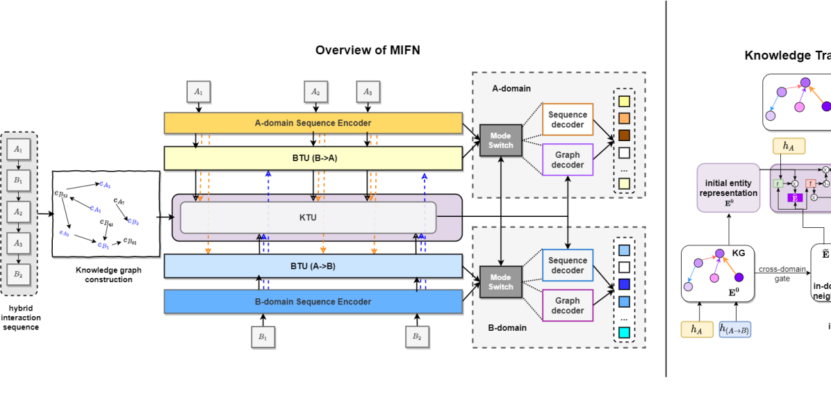
As shown in the left side of Figure 2, MIFN consists of four main components: a sequence encoder, a behavior transfer unit (BTU), a knowledge transfer unit (KTU), and a mixed recommendation decoder. The sequence encoder encodes the interacted item sequence into a sequence of item representations. The BTU takes the representations from the source domain as input, extracts behavioral information flow, and transfers it to the target domain. The KTU aims to grasp useful knowledge from the KG and propagates it to both domains. The mixed recommendation decoder contains two decoders w.r.t. graph mode and sequence mode, respectively. The graph recommendation decoder evaluates the probability for all candidate items from the KG, corresponding to Eq. LABEL:g_rec. The sequence recommendation decoder evaluates the probability of clicking items, corresponding to Eq. LABEL:s_rec.

3.4. Sequence encoder

As with existing studies (Hidasi et al., 2016a, b), we use an RNN to encode the sub-sequences $S_{A}$ and $S_{B}$. Here, we employ a GRU as the recurrent unit. The initial state of the GRUs is set to zero vectors, i.e., $h_{0}=0$. After that, we can obtain $H_{A}=\{h_{A_{1}}$, $h_{A_{2}}$, …, $h_{A_{i}}$, …, $h_{A_{n}}\}$ for domain $A$, and $H_{B}=\{h_{B_{1}},h_{B_{2}},\ldots,h_{B_{j}},\ldots,h_{B_{m}}\}$ for domain $B$. Each $h_{A_{i}}$ or $h_{B_{j}}$ is the item representation of an item $A_{i}$ in sequence $S_{A}$ or $B_{j}$ in $S_{B}$.

3.5. Behavior transfer unit

The outputs $H_{A}$ and $H_{B}$ from the sequence encoder are representations of user behavior in single domains. It has been shown that there is connection between $H_{A}$ and $H_{B}$ (Ma et al., 2019a). For example, a user who has read the Harry Potter book (e.g., “Harry Potter and the Philosopher’s Stone” or “Harry Potter and the Chamber of Secrets” and so on) has also watched the “Pirates of the Caribbean” movie within the same time period. Based on behavioral information from both domains, it is easier for the model to infer that the user might like some magic and fantastic movies and books.

To achieve this, we employ the BTU to model the flow of behavioral information from domain $A$ to domain $B$, i.e., $h_{A_{i}\rightarrow B}$, as follows:

(3) $$\begin{split}f_{A_{i}}&{}=\sigma(W_{f_{A}}\cdot h_{A_{i}}+W_{f_{B}}\cdot h_{B_{j}}+W_{f}\cdot h_{A_{i-1}\rightarrow B}+b_{f})\\ \widehat{h_{A_{i}}}&{}=\tanh({W_{h}\cdot h_{A_{i}}+U_{h}\cdot h_{A_{i-1}\rightarrow B}+b_{h}})\\ h_{A_{i}\rightarrow B}&{}=f_{A_{i}}\odot\widehat{h_{A_{i}}}+(1-f_{A_{i}})\odot h_{A_{i-1}\rightarrow B},\end{split}$$

where $h_{A_{i}}$ and $h_{B_{j}}$ are the representations of domain $A$ and $B$ at timestamp $i$ and $j$, respectively. $f_{A_{i}}$ measures the degree of connection between these two representations $h_{A_{i}}$ and $h_{B_{j}}$ from both domains, which employs the gate mechanism to control how much information is to be transferred from domain $A$ to domain $B$. $\widehat{h_{A_{i}}}$ is the updated representation of the current input. $W_{A}$ and $W_{B}$ are the parameters, $b_{f}$ is the bias term, $\odot$ indicates element-wise multiplication. $h_{A_{i}\rightarrow B}$ can be seen as a combination of $\widehat{h_{A_{i}}}$ and $h_{A_{i-1}\rightarrow B}$ balanced by $f_{A_{i}}$. Note that the BTU can be applied bidirectionally from “domain $A$ to domain $B$” and “domain $B$ to domain $A$”. Here, we take the “domain $A$ to domain $B$” direction and achieve recommendations in domain $B$ as an example.

$h_{A_{i}\rightarrow B}$ is the information extracted from domain $A$, which is ready to be transferred to domain $B$. Since it still belongs to domain $A$, we employ an RNN structure to transfer it to domain $B$ as follows:

(4) $$\begin{split}&h_{(A\rightarrow B)_{i}}=GRU(h_{(A\rightarrow B)_{i-1}},h_{A_{i}\rightarrow B}).\\ \end{split}$$

After that, we can obtain the transferred behavioral representation $h_{(A\rightarrow B)_{i}}$ in domain $B$ at time step $i$.

3.6. Knowledge transfer unit

The BTU only models the flow of behavioral information. We hypothesize that this may be not enough for the model to be able to encode the connection between items from the two domains in some cases. For example, if there is no knowledge indicating that both “Pirates of the Caribbean” and “Harry Potter” belong to fantasy, it is difficult for the model to capture the connection between them solely based on behavioral information. To better transfer the information of items from both domains, we propose the KTU, as shown in the right side of the Figure 2.

For each hybrid interaction sequence $S$, we get the item representations $\{h_{A_{1}}$, $h_{A_{2}}$, …, $h_{A_{i}},\ldots\}$ from the sequence encoder (Section 3.4) and the transferred behavioral representations $\{h_{(A\rightarrow B)_{1}}$, $h_{(A\rightarrow B)_{2}},\ldots,h_{(A\rightarrow B)_{i}},\ldots\}$ from the BTU (Section 3.5). We use the item representation of the last time step to denote the sequence representation $h_{A}$ and the transferred behavioral representation $h_{(A\rightarrow B)}$. We also obtain the relational adjacency matrix $A$ of the KG, which consists of $N$ entities and the corresponding relations (§3.2). Here, we represent these $N$ entities as $E$, the corresponding relations are represented as $R$.

We initialize all entities in the KG and we can get the initialized entity representations $h_{E^{0}}$. That is, for each entity $e_{k}\in E$, the initialized entity representation is $h_{e_{k}^{0}}\in h_{E^{0}}$. Then we learn a transferred entity representation $h_{e_{k}^{T}}\in h_{E^{T}}$ for each entity $e_{k}$ by leveraging the relations in the KG, as shown in Eq. 5:

(5) $$\begin{split}r&=\sigma(W_{r}\cdot h_{e_{k}^{0}}+U_{r}\cdot\widetilde{h_{e^{L}_{k}}}+b_{r})\\ f&=\sigma(W_{f}\cdot h_{e_{k}^{0}}+U_{f}\cdot\widetilde{h_{e^{L}_{k}}}+V_{f}\cdot h_{A}+b_{f})\\ \widehat{h_{e_{k}}}&=\tanh(W_{h}\cdot\widetilde{h_{e^{L}_{k}}}+U_{h}\odot(r\odot h_{e_{k}^{0}}))\\ h_{e_{k}^{T}}&=(1-f)\odot h_{e_{k}^{0}}+f\odot\widehat{h_{e_{k}}}.\\ \end{split}$$

The explanations for the main parts of Eq. 5 are as follows:

1. Gated functions. $r$ and $f$ are the update gate function and the forget gate function, which aim to regulate how much of the update information should be propagated. $W_{r}$, $U_{r}$, $W_{f}$, $U_{f}$ and $V_{f}$ are the parameters; $b_{r}$ and $b_{f}$ are the bias term.

2. Candidate knowledge transfer representation. $\widehat{h_{e_{k}}}$ is the candidate knowledge transfer representation, which is calculated based on the cross-domain disseminated entity representation $\widetilde{h_{e^{L}_{k}}}$ at the $L$-th hop layer (we will explain this later in Eq. 6) and the updated entity representation $r\odot h_{e_{k}^{0}}$. $W_{h}$ and $U_{h}$ are the parameters, $\odot$ indicates element-wise multiplication.

3. Transferred entity representation. The transferred entity representation $h_{e_{k}^{T}}$ is a combination of the initialized entity representation $h_{e_{k}^{0}}$ and the candidate knowledge transfer representation $\widehat{h_{e_{k}}}$ balanced by the forget gate $f$, where the information among entities has been disseminated through $L$ hop layers.

Graph convolutional techniques are commonly used to disseminate information among entities based on their relations (Kipf and Welling, 2017; Wang et al., 2019d; Wang et al., 2018). However, in the cross-domain scenario that we consider, the information disseminated by entities from different domains is different. Hence, we propose a cross-domain graph convolutional mechanism that can distinguish entities from different domains and adopt different modeling methods to disseminate their information so as to get better entity representation. In this manner, the information in the KG is disseminated between both domains, which can be considered as a flow of knowledge in the hybrid interaction sequence. Suppose the information can be disseminated within $L$ hop layers. At the $l$-th hop layer ($0\leq l\leq L$), the information of each entity and its cross-domain neighbor entities via various relations will be disseminated to the next hop layer $l+1$ and is used to update the entity representation. The process of cross-domain information dissemination is defined in Eq. 6:

(6) $$\begin{split}\mbox{}\widetilde{h_{e^{l+1}_{k}}}=\sigma\left[f_{0}(\widetilde{h_{e^{l}_{k}}})+\frac{1}{|N_{i}(k)|}\sum_{r\in R}\sum_{p\in N_{i}(k)}f_{i}(\alpha_{p}\cdot\widetilde{h_{e^{l}_{p}}})+\frac{1}{|N_{c}(k)|}\sum_{r\in R}\sum_{q\in N_{c}(k)}f_{c}(\beta_{q}\cdot\widetilde{h_{e^{l}_{q}}}+c_{q}\cdot\widetilde{h_{e^{l}_{q}}})\right],\mbox{}\end{split}$$

where $e_{k}$ is any entity in the entity set $E$; $N_{i}(k)$ is the neighbor entity set of entity $e_{k}$ from the same domain as $e_{k}$; $N_{c}(k)$ is the neighbor entity set of entity $e_{k}$ from the complementary domain. $f_{0}$, $f_{i}$ and $f_{c}$ represent the transformation functions for initialization, in-domain and cross-domain respectively; $\alpha_{p}$ is the in-domain attention weight calculated between each entity $e_{p}\in N_{i}(k)$ and the sequence representation $h_{A}$; $\beta_{q}$ is the cross-domain attention weight calculated between each entity $e_{q}\in N_{c}(k)$ and the transferred behavioral representation $h_{(A\rightarrow B)}$; $c_{q}$ shows the sum of similarities between entity $e_{q}$ and each entity $e_{p}\in N_{i}(k)$, which is defined as: $c_{q}=\sum_{p\in N_{i}(k)}e_{p}\cdot e_{q}$; $\widetilde{h_{e^{l}_{k}}}$ denotes the cross-domain disseminated representation of entity $e_{k}$ at the $l$-th hop layer, which aggregates the information from itself and cross-domain neighbor entities as the new representation for the next hop layer. At the first hop layer, the cross-domain disseminated representation is assigned by the gated entity representation, i.e., $\widetilde{h_{e^{0}_{k}}}=h_{e_{A_{k}}}$ if the entity $e_{k}$ is from domain $A$, otherwise $\widetilde{h_{e^{0}_{k}}}=h_{e_{B_{k}}}$:

(7) $$\begin{split}c&=\sigma\left(W_{c}\cdot concat[h_{A},h_{(A\rightarrow B)},h_{E_{0}}]+b_{c}\right)\\ h_{e_{A_{k}}}&=c\odot\left(\alpha_{A_{k}}\cdot h_{e_{A_{k}}^{0}}\right)\\ h_{e_{B_{k}}}&=(1-c)\odot\left(\beta_{B_{k}}\cdot h_{e_{B_{k}}^{0}}\right),\\ \end{split}$$

where $W_{c}$ is the parameter; $b_{c}$ is the bias term; $h_{e_{A_{k}}}$ is the gated entity representation of entity $e_{A_{k}}\in E_{A}$, $h_{e_{B_{k}}}$ is the gated representation of entity $e_{B_{k}}\in E_{B}$. $c$ is a cross-domain information gate to handle the situation where the proportion of entities from different domains in the KG is different (e.g., when there are 1000 entities from domain $A$, but only 10 entities from domain $B$). So we define the gated entity representations $h_{e_{A_{k}}}$ for domain $A$ and $h_{e_{B_{k}}}$ for domain $B$ based on their initial entity representations respectively, which aims to balance information from both domains. $\alpha_{A_{k}}$ is the attention weight of $e_{A_{k}}$ for sequence representation $h_{A}$; $\beta_{B_{k}}$ is the attention weight of $e_{B_{k}}$ for the transferred behavioral representation $h_{(A\rightarrow B)}$. These attention weights act as an information controller to identify entities of different importance in the KG, the definitions of which are shown in Eq. 8:

(8) $$\begin{split}s_{A_{k}}&=\mathbf{v_{1}}^{\mathsf{T}}\tanh{\left(W_{A_{1}}\cdot h_{A}+W_{A_{2}}\cdot h_{e_{A_{k}}^{0}}\right)}\\ \alpha_{A_{k}}&=\frac{\exp{(s_{A_{k}})}}{\sum_{i}\exp{(s_{A_{i}}})}\\ s_{B_{k}}&=\mathbf{v_{2}}^{\mathsf{T}}\tanh{\left(W_{B_{1}}\cdot h_{(A\rightarrow B)}+W_{B_{2}}\cdot h_{e_{B_{k}}^{0}}\right)}\\ \beta_{B_{k}}&=\frac{\exp{(s_{B_{k}})}}{\sum_{j}\exp{(s_{B_{j}}})},\\ \end{split}$$

where $h_{e_{A_{k}}^{0}}$ and $h_{e_{B_{k}}^{0}}$ are the initialized entity representations of entity $e_{A_{k}}$ and $e_{B_{k}}$ respectively. $h_{A}$ is the sequence representation and $h_{(A\rightarrow B)}$ is the transferred behavioral representation as mention above. $\mathbf{v_{1}}$, $\mathbf{v_{2}}$, $W_{A_{1}}$, $W_{A_{2}}$, $W_{B_{1}}$ and $W_{B_{2}}$ are learnable parameters.

3.7. Mode switch

Recall that $P(M\_S_{B}|S,\langle E,R\rangle)$ and $P(M\_G_{B}|S,\langle E,R\rangle)$ are the probabilities of conducting recommendations under sequence mode and graph mode, respectively. We model the mode switch as a binary classifier. Specifically, we first combine the sequence representation $h_{B}$, the transferred behavioral representation $h_{(A\rightarrow B)}$ and the sum of all transferred entity representation $\sum_{k}(h_{e_{k}^{T}})$ (where $h_{e_{k}^{T}}\in h_{E^{T}}$). Then, we employ a softmax regression to transform the total representation into the mode probability distributions, as follows:

(9) $$\begin{split}P(M\_G_{B}|S,\langle E,R\rangle),P(M\_S_{B}|S,\langle E,R\rangle)=\text{softmax}\left(W_{m}\cdot concat\left[h_{B},h_{(A\rightarrow B)},\sum_{k}(h_{e_{k}^{T}})\right]+b_{m}\right),\end{split}$$

where $W_{m}$ is the weight matrix and $b_{m}$ is the bias term.

3.8. Graph recommendation decoder

The graph recommendation decoder evaluates the probabilities of recommending items involved in the KG. Here we directly use the representations of entities to learn the attention weights and take these weights as the final predicted recommendation probability. The recommendation probability for each item $B_{j+1}\in E_{B}$ is computed as follows:

(10) $$\begin{split}&P(B_{j+1}|M\_G_{B},S,\langle E,R\rangle)=\begin{cases}0&\text{if }{B_{j+1}\notin\mathbbm{B}}\\ \frac{\exp(h_{e_{B_{j+1}}^{T}})}{\sum_{k}^{m}\exp(h_{e_{k}^{T}})}&\text{if }{B_{j+1}\in\mathbbm{B}},\end{cases}\end{split}$$

where $h_{e_{B_{j+1}}^{T}}$ is the transferred entity representation of $e_{B_{j+1}}$ (corresponding to $h_{e_{k}^{T}}$ in Eq. 5 when $e_{k}$ is an item entity from domain $B$). $m$ is the number of the item set $\mathbbm{B}$. Note that $e_{B_{j+1}}\in E_{B}$ is an item entity corresponding to item $B_{j+1}\in\mathbbm{B}$. The recommendation probabilities are set to zero for those items that do not exist in $\mathbbm{B}$.

3.9. Sequence recommendation decoder

The sequence recommendation decoder evaluates the probabilities of items in the sequence item set. We first concatenate the sequence representation $h_{B}$ and the transferred behavioral representation $h_{(A\rightarrow B)}$ into the hybrid representation $c_{S}$, i.e., $c_{S}=\begin{bmatrix}h_{B},h_{(A\rightarrow B)}\\ \end{bmatrix}^{\mathsf{T}}$. Then, the recommendation probability for each item $B_{j+1}\in\mathbbm{B}$ is computed as follows:

(11) $$\begin{split}&P(B_{j+1}|M\_S_{B},S,\langle E,R\rangle)=\begin{cases}0&\text{if }{B_{j+1}\notin\mathbbm{B}}\\ \frac{\exp(W_{j+1}c_{S}+b_{I})}{\sum_{k}^{m}\exp(W_{k}c_{S}+b_{I})}&\text{if }{B_{j+1}\in\mathbbm{B}},\end{cases}\end{split}$$

where $W_{k}\in W_{I}$ is the weight matrix, $b_{I}$ is the bias term. The recommendation probabilities are set to zero for those items that do not exist in the item set $\mathbbm{B}$.

3.10. Objective function

Our goal is to maximize the prediction probability for each domain given a hybrid interaction sequence. Therefore, we define the negative log-likelihood loss function as follows:

(12) $$L_{R}(\theta)=L_{R_{A}}(\theta)+L_{R_{B}}(\theta),$$

where $\theta$ are all parameters in MIFN. Specifically, $L_{R_{A}}(\theta)$ and $L_{R_{B}}(\theta)$ can be derived as follows:

(13) $$\begin{split}L_{R_{A}}(\theta)&=-\frac{1}{|\mathbb{S}|}\sum_{S\in\mathbb{S}}\sum_{A_{i}\in S}\log P(A_{i+1}|S,\langle E,R\rangle)\\ L_{R_{B}}(\theta)&=-\frac{1}{|\mathbb{S}|}\sum_{S\in\mathbb{S}}\sum_{B_{j}\in S}\log P(B_{j+1}|S,\langle E,R\rangle),\end{split}$$

where $\mathbb{S}$ is the set of all hybrid interaction sequences in our training set, and $P(A_{i+1}|S,\langle E,R\rangle)$ or $P(B_{j+1}|S,\langle E,R\rangle)$ are the next prediction probabilities, which are as defined in Eq. 2.

Additionally, MIFN incorporates a mode switch module to calculate the mode selection probability between sequence mode and graph mode. We assume that if an item does not exist in item set, it can just be generated under the graph mode. Here, we can jointly train another mode prediction loss as follows, which adopts the negative log-likelihood loss:

(14) $$\begin{split}L_{M_{A}}(\theta)&=-\frac{1}{|\mathbb{S}|}\sum_{S\in\mathbb{S}}\sum_{A_{i}\in S}[(1-\mathbbm{1}(A_{i+1}\in\mathbbm{A}))\log P(M\_S_{A}|S,\langle E,R\rangle)]\\ L_{M_{B}}(\theta)&=-\frac{1}{|\mathbb{S}|}\sum_{S\in\mathbb{S}}\sum_{B_{j}\in S}[(1-\mathbbm{1}(B_{j+1}\in\mathbbm{B}))\log P(M\_S_{B}|S,\langle E,R\rangle)]\\ L_{M}(\theta)&=L_{M_{A}}(\theta)+L_{M_{B}}(\theta),\\ \end{split}$$

where $\mathbbm{1}(item\in itemset)$ is the indicator function that equals 1 if this item is in the item set and 0 otherwise. $L_{M}(\theta)$ is the total mode loss for domain $A$ and $B$.

Finally, we adopt a joint-learning strategy, and the final loss combines both recommendation loss and mode loss:

(15) $$\begin{split}&L(\theta)=L_{R}(\theta)+L_{M}(\theta).\\ \end{split}$$

4. Experimental Setup

4.1. Research questions

We evaluate MIFN on four e-commerce datasets. We aim to answer the following questions in our experiments:

1. How does MIFN perform compared with the state-of-the-art methods in terms of Recall and MRR? (See Section 5.1.)

2. Does the KTU help to improve the performance of recommendations? And does the performance differ from the situation when we only allow for the flow of behavioral information? (See Section 5.2.)

3. Does the knowledge graph construction method have a big effect on the overall recommendation results? (See Section 5.3.)

4. Is MIFN able to provide better recommendations by incorporating the flow of knowledge across domains? (See Section 5.4.)

4.2. Datasets

We conduct experiments on the Amazon e-commerce collection, which consists of user interactions (e.g., userid, itemid, ratings, timestamps) from multiple domains and some item meta information (e.g., descriptions, images, product associations). Compared with other recommendation datasets, the Amazon dataset contains overlapping user interactions in multiple domains, which is suitable for cross-domain sequential recommendation (CDSR). Specifically, we pick two pairs of complementary domains “Movie-Book” domains and “Food-Kitchen” domains for experiments. For the “Movie-Book” dataset, the “Movie” domain contains movie watching records. The “Book” domain covers book reading records. For the “Food-Kitchen” dataset, the “Food” domain contains food purchase records. The “Kitchen” domain contains furniture purchase records. We follow the settings of Ma et al. (2019a) to process the data. To satisfy cross-domain characteristics, we first pick users who have interactions in both domains. Since we do not target cold-start users or items in this work, we only keep users who have more than 10 interactions and items whose frequency is larger than 10. To satisfy sequential characteristics which consists of many user interactions within a period of time, we first order the interactions by time for each user, then we split the sequences from each user into several small sequences with each sequence containing interactions within a period, i.e., a month for the “Movie-Book” dataset, and a year for the “Food-Kitchen” dataset. We also require that each sequence contains at least 3 items from each domain. The statistics of the processed datasets are shown in Table 2.

Table 2. Dataset statistics.

Domain	#Items	#Train	#Test	#Valid	Avg_Seq_Len
Movie	36,845	44,732	19,861	9,274	11.98
Book	63,937
Food	29,207	25,766	17,280,	7,650	19.91
Kitchen	34,886

For knowledge graph construction, we use the Amazon product data to mine the relations of the items. The data is collected from large-scale user logs, which contain the following relations: (1) “Also_buy” (users also buy item $X$ when buying item $Y$.); (2) “Also_view” (users also view item $X$ when viewing item $Y$.); (3) “Buy_together” (users buy item $X$ and $Y$ together frequently); (4) “Buy_after_viewing” (users buy item $X$ after they buy $Y$); (5) “Is_the_same_category” (item $X$ and $Y$ belong to the same category). Additionally, for the “Movie-Book” dataset, we also crawl the relation “Adapted_from” between books and movies from Wikipedia. For example, $\langle$movie, Adapted_from, book$\rangle$ means that the movie is adapted from the book. We align knowledge entities with Wikipedia titles by fully matching. The statistics of the knowledge information are shown in Table 3.

Table 3. KG statistics.

Domain	#Entities	#Relations	#Triples
Movie	065,418	6	03,911,284
Book	315,770		40,048,795
Food	050,273	5	03,822,123
Kitchen	082,552		07,836,064

For evaluation, we use the last interacted item in each sequence for each domain as the ground truth item, respectively. We randomly select 80% of each user’s interactions as the training set, 10% as the validation set, and the remaining 10% as the test set.

4.3. Baseline methods

We compare the proposed model MIFN with baselines from five categories: (1) traditional recommendation methods, (2) cross-domain recommendation methods, (3) sequential recommendation methods, (4) cross-domain sequential recommendation methods, and (5) knowledge-aware recommendation methods.

4.3.1. Traditional recommendation methods.

We adapt three commonly used traditional recommendation methods to SRs:

• POP: This method recommends the most popular items in which items are ranked based on their popularity. It is a simple baseline, but is commonly used owing to its simplicity yet effectiveness (He et al., 2017).

• Item-KNN: This method is inspired by the classical KNN model; it looks for items that are similar to other items that have been clicked by a user in the past, where similarity is defined as the cosine similarity between the vector of sequences (Sarwar et al., 2001).

• BPR-MF: This method follows the idea of MF with a pairwise ranking objective via stochastic gradient descent (Rendle et al., 2009). Following Hidasi et al. (2016a), we represent a new sequence by the average latent factors of items that appeared in the sequence so far.

4.3.2. Cross-domain recommendation methods.

We use two popular cross-domain recommendation methods for comparison.

• NCF-MLP++: This is a deep learning based method where the model learns the inner product of the traditional CF by using multilayer perceptron (MLP) in each domain. The user representations are shared between both domains while item representations are private in each domain, and the final recommendations are aggregated from both domain recommendations probabilities. We adopt the implementation in (Ma et al., 2019a).

• Conet: This method transfers information between different domains by a cross-stitch network (Misra et al., 2016), where information in each domain is captured by neural CF model (He et al., 2017).

4.3.3. Sequential recommendation methods.

A number of SR methods have been proposed in the last few years. In this work, we construct/select baselines that are fair (use the same information, similar architectures, etc.) to compare with:

• GRU4REC: It is the first attempt to use GRU for SRs. It utilizes session-parallel mini-batch training strategy and employs a ranking-based loss functions (Hidasi et al., 2016a).

• HRNN: This method combines the extra user’s information into GRU networks and proposes a hierarchical RNN model based on GRU4REC (Quadrana et al., 2017).

• NARM: This method takes an attention mechanism into consideration to capture both sequential-level preferences and the user’s main purpose (Li et al., 2017).

• STAMP: This method constructs two network structures to capture a user’s general preferences and the current preferences of the last click within the current sequence (Liu et al., 2018).

4.3.4. Cross-domain Sequential recommendation methods.

• $\pi$-Net: This method is the only one that considers cross-domain characteristics for SRs. We take this as the fairest baseline to compare with. It designs a new gating mechanism to recurrently extract and share useful information across different domains (Ma et al., 2019a).

4.3.5. Knowledge-aware recommendation methods.

• SRGNN: This method constructs each sequence as a directed graph, where the items in the sequence are entities and transition relationship between adjacent items represents edge which is considered as knowledge information. By modeling the complex transitions, each session graph and item embeddings of all items involved in each graph can be obtained through gated graph neural networks (Wu et al., 2019).

• KSR: This method incorporates KGs into SRs, and it combines the sequential user preference captured by an RNN and attribute-level preferences captured by Key-Value Memory Networks to get the final representation of user preference (Huang et al., 2018).

4.4. Evaluation metrics

We target the top-K recommendations in this work, so we adopt two widely used ranking-based metrics (Cheng et al., 2018; He et al., 2018; Mei et al., 2018; Ren et al., 2019): MRR@K and Recall@K. Specifically, we report $K$ = 5, 10, 20.

• Recall: This measures the proportion of the top-K recommended items that are in the evaluation set. It does not consider the actual rank of the item as long as it is amongst the list of recommend items.

• MRR: This is the average of reciprocal ranks of the relevant items. And the reciprocal rank is set to zero if the ground truth item is not in the list of recommended items. MRR takes the order of recommendation ranking into account. Since each sample has only one ground truth item, we choose MRR as the ranking metric instead of others, e.g., NDCG.

4.5. Implementation details

For most of the baseline methods, we find the best settings using grid search on the validation set. For those with too many hyperparameters, we follow the reported optimal hyperparameter settings from the original publications that introduced them. For our model, the embedding size and the hidden size are set to 256, the hop layer $H$ is set to 2, and the number of entities $N$ in KG is set to 200. We initialize the model parameters randomly using the Xavier method. We take Adam as our optimization method. MIFN is implemented in TensorFlow and trained on a GeForce GTX TitanX GPU. The code and dataset used to run the experiments in this paper are available at https://github.com/mamuyang/MIFN.

5. Results and Analysis

5.1. Overall performance (RQ1)

We report the results of MIFN compared with the baseline methods on the “Movie-Book” and “Food-Kitchen” datasets. The results of all methods are shown in Table  4 and  5, respectively. From the results, we have the following main observations.

Table 4. Experimental results (%) on the Amazon (“Movie-Book”) dataset. Bold face indicates the best result in terms of the corresponding metric. Significant improvements over the best baseline results are marked with ^† (t-test, $p<.05$).

Methods	Movie-domain						Book-domain
	MRR			Recall			MRR			Recall
	@5	@10	@20	@5	@10	@20	@5	@10	@20	@5	@10	@20
POP	00.10	00.11	00.13	00.20	00.29	00.58	00.11	00.14	00.16	00.20	00.44	00.75
BPR-MF	00.51	00.57	00.64	00.89	01.35	02.26	01.44	01.64	01.77	02.51	03.97	05.97
ItemKNN	01.05	01.27	01.48	02.11	03.84	06.99	01.35	01.64	01.95	02.88	05.10	09.69
NCF-MLP++	01.64	01.86	02.03	02.95	04.61	07.24	01.76	01.98	02.11	03.20	04.84	07.34
Conet	01.43	01.73	02.01	02.83	05.20	09.24	01.17	01.36	01.51	02.13	03.54	05.77
GRU4REC	12.80	12.86	12.88	13.69	14.11	14.43	13.87	13.92	13.95	14.64	15.02	15.34
HRNN	13.38	13.43	13.45	13.95	14.25	14.58	14.57	14.61	14.62	14.99	15.25	15.46
NARM	13.80	13.85	13.86	14.20	14.53	14.80	15.25	15.26	15.27	15.57	15.66	15.78
STAMP	12.44	12.56	12.63	13.66	14.58	15.68	11.53	11.56	11.57	11.82	12.00	12.20
$\pi$-Net	14.49	14.52	14.54	14.88	15.10	15.37	15.75	15.76	15.77	15.94	16.02	16.09
SRGNN	11.77	11.84	11.88	12.66	13.18	13.87	15.12	15.14	15.15	15.46	15.61	15.77
KSR	14.18	14.23	14.26	14.91	15.28	15.73	15.84	15.87	15.89	16.51	16.72	16.92
MIFN-KTU	14.20	14.25	14.28	14.85	15.26	15.44	14.87	14.90	14.91	15.54	15.80	16.07
MIFN+$L_{M}$	14.73	14.75	14.81	14.87	15.96	16.02	15.75	15.97	15.99	16.87	16.96	17.05
MIFN	14.84	14.87	14.88	15.13	16.34†	16.56†	16.05	16.16	16.23†	16.99†	17.03†	17.13†

First, MIFN outperforms the single-domain SR methods (e.g., STAMP, NARM) and the knowledge-aware methods (e.g., SRGNN, KSR) on all datasets. Particularly, on the “Movie-Book” dataset, the largest increase over NARM is 7.5% and 12.4% in terms of MRR@5 and Recall@10 on the “Movie” domain, and on the “Book” domain, the largest increase is 6.2% and 9.1% in terms of MRR@20 and Recall@5. And the increase over KSR on the “Movie” domain is 4.6% and 6.9% in terms of MRR@5 and Recall@10, on the “Book” domain, the increase is 2.1% and 2.9% in terms of MRR@20 and Recall@5. On the “Food-Kitchen” dataset, the largest increase over NARM is 6.5% and 9.3% in terms of MRR@20 and Recall@20 on the “Food” domain, and on the “Kitchen” domain, the increase is 9.1% and 12.3% in terms of MRR@5 and Recall@10. And the increase over KSR is 2.7% and 3.9% in terms of MRR@20 and Recall@10 on the “Food” domain, and on the “Kitchen” domain, the increase is 1.6% and 4.1% in terms of MRR@20 and Recall@20. These improvements demonstrate that jointly considering both cross-domain behavior and knowledge is helpful for SR.

Table 5. Experimental results (%) on the Amazon (“Food-Kitchen”) dataset. Bold face indicates the best result in terms of the corresponding metric. Significant improvements over the best baseline results are marked with ^† (t-test, $p<.05$).

Methods	Food-domain recommendation						Kitchen-domain recommendation
	MRR			Recall			MRR			Recall
	@5	@10	@20	@5	@10	@20	@5	@10	@20	@5	@10	@20
POP	00.40	00.49	00.56	00.82	01.50	02.15	00.22	00.25	00.27	00.40	00.60	01.47
BPR-MF	00.82	00.87	00.94	01.35	01.82	02.61	00.41	00.47	00.50	00.62	01.04	01.47
ItemKNN	01.55	01.98	02.43	03.28	06.70	12.47	01.13	01.44	01.90	02.60	04.77	11.08
NCF-MLP++	02.01	02.24	02.42	03.45	05.19	08.02	00.87	01.03	01.17	01.72	03.00	04.99
Conet	03.38	03.64	03.82	05.07	07.07	09.73	03.30	03.55	03.71	05.09	07.03	09.47
GRU4REC	08.10	08.23	08.29	09.46	10.38	11.26	08.36	08.39	08.41	08.70	08.93	09.25
HRNN	07.22	07.35	07.45	08.49	09.47	10.93	07.81	07.86	07.88	08.29	08.61	09.12
NARM	09.43	09.54	09.62	10.34	11.86	12.23	08.41	08.44	08.46	08.69	08.91	09.21
STAMP	09.28	09.38	09.44	10.22	10.91	11.81	08.52	08.55	08.57	08.81	09.05	09.28
$\pi$-Net	09.56	09.67	09.75	10.59	10.46	12.54	08.57	08.60	08.62	08.89	09.12	09.42
SRGNN	07.31	07.49	07.60	08.68	10.02	11.67	07.20	07.26	07.29	07.90	08.36	08.87
KSR	09.79	09.91	09.98	10.82	11.78	12.77	09.03	09.07	09.08	09.39	09.62	09.92
MIFN-KTU	09.43	09.65	09.83	10.50	11.16	12.53	08.29	08.33	08.36	08.95	09.17	09.52
MIFN+$L_{M}$	09.86	09.88	10.03	10.93	11.96	13.14	09.05	09.17	09.18	09.28	09.89	10.24
MIFN	09.91	10.16	10.25	11.20	12.25	13.27†	09.18	09.21	09.23	09.72†	10.01†	10.33†

Second, MIFN outperforms the cross-domain sequential recommendation baseline $\pi$-Net, which just makes use of information at user behavior level. Specifically, MIFN outperforms $\pi$-Net in terms of all metrics on both domains. It demonstrates that considering both knowledge and user behavior level information is better than only behavioral information. Meanwhile, it also proves the effectiveness of the KTU module of MIFN. With this module, MIFN is able to capture cross-domain knowledge and conduct information transfer in the KG so as to learn better sequence representations.

Third, we can observe that the results of MIFN in the “Book” domain are better than those in the “Movie” domain on the “Movie-Book” dataset. We believe that this is because the data is less sparse in the “Book” domain compared to that in the “Movie” domain. And the results in the “Food” domain are better than the “Kitchen” domain on the “Food-Kitchen” dataset. Again, we think it is because the data sparsity difference as the users have more interactions in the “Food” domain than in the “Kitchen” domain. With more interaction data, the models can identify more user preference characteristics in the dense domain so as to transfer it to the sparse domain through both the user behavioral information flow and the knowledge information flow.

Fourth, $\pi$-Net outperforms other sequential baselines, which means that cross domain information is beneficial to both domains. At the same time, knowledge aware methods outperform other sequential baselines, which also means that knowledge information can improve recommendation performance. Furthermore, it seems that considering knowledge is more useful than modeling cross-domain characteristics, as KSR slightly outperforms $\pi$-Net.

Fifth, the sequential methods achieve much better results than traditional methods and cross-domain methods. This is because RNN-based methods are able to capture the sequential characteristics and can obtain the better representations while the traditional methods neglect this information. Besides, it seems that STAMP obtains lower results than the sequential method NARM in the “Movie-Book” dataset, while it performs better in the “Kitchen” domain of “Food-Kitchen” dataset. We believe that this is because of differences in the datasets, e.g., we found that the user preferences in the kitchen domain are relatively more focused. And the knowledge aware method SRGNN performs worse than most sequential methods. This is because that SRGNN just employs the transition relation between adjacent items to construct the graph so as to get the representations of different items, however it does not consider the relation between the non-adjacent items (the other sequential methods do consider this), which may also affect item representations.

5.2. Ablation study (RQ2)

To verify the effectiveness of the proposed modules, we design the ablation study to compare several model variants. The results are listed in Table 4 and Table 5.

1. MIFN is the best performing variant, which includes both the BTU and KTU modules, and trained with the recommendation loss $L_{R}$ only.

2. MIFN-KTU is MIFN without the KTU module and performs information transfer only at the level of behavioral information;

3. MIFN+$L_{M}$ is MIFN by adding the mode switch loss.

First, by removing KTU, the performance of MIFN-KTU is dramatically less than that of MIFN, which confirms that considering knowledge flow can improve the cross-domain recommendations. In addition, the results of MIFN-KTU are worse than those of the knowledge-aware method KSR, while MIFN outperforms KSR on all domains. This indicates that the KTU module is able to make good use of the cross-domain knowledge and is able to better capture user preferences by modeling the cross-domain knowledge flow.

Second, if we jointly train the recommendation loss $L_{R}$ and the mode switch loss $L_{M}$, the performance drops a little but its performance is still than that of the baselines. The switch loss $L_{M}$ assumes that if the next item does not exist in the item set, it must be recommended under the graph mode, which makes the model tend to recommend items existing in the graph. However, since there already exists a similar supervision signal in $L_{R}$, which assumes that each item is recommended under the graph mode, the sequence mode, or a combination of both. Further adding the $L_{M}$ loss introduces unnecessary bias towards graph mode.

5.3. Influence of the knowledge graph construction algorithm (RQ3)

The number of triples in the complete KG is large (see Table 3), so we propose a knowledge graph construction method as detailed in Algorithm 1 to build KG for each sequence. To study the effect of the knowledge graph construction method, we design an experiment aimed at analyzing the effect of the ratios of the ground truth items in the constructed KG on the final recommendation performance. We achieve this by simulating and controlling the ratios artificially. Specifically, we add the ground truth items to the extracted entities according to the specified ratios in advance. The results are shown in Table 6 and Table 7.

Table 6. Analysis of the knowledge graph construction algorithm on the Amazon (“Movie-Book”) dataset. The different ratios represent the different proportions of the predicted ground truth items appeared in the KG.

Ratios	Movie-domain recommendation						Book-domain recommendation
	MRR			Recall			MRR			Recall
	@5	@10	@20	@5	@10	@20	@5	@10	@20	@5	@10	@20
30%	16.46	16.83	16.99	21.27	24.33	28.97	18.51	18.70	18.85	25.82	27.32	31.38
50%	19.53	20.43	20.83	30.33	37.07	42.67	25.04	25.68	25.98	36.08	40.75	45.12
70%	23.41	23.43	23.45	42.54	47.99	50.61	27.12	28.31	28.41	48.93	56.64	57.31
90%	33.45	34.99	35.09	65.81	76.83	77.97	40.01	40.86	43.00	79.83	80.50	83.86
100%	67.04	67.56	67.69	89.57	93.30	95.15	83.08	83.46	83.62	91.97	94.79	97.02

Table 7. Analysis of the knowledge graph construction algorithm on the Amazon (“Food-Kitchen”) dataset. The different ratios represent the different proportions of the predicted ground truth items appeared in the KG.

Ratios	Food-domain recommendation						Kitchen-domain recommendation
	MRR			Recall			MRR			Recall
	@5	@10	@20	@5	@10	@20	@5	@10	@20	@5	@10	@20
30%	11.75	12.30	12.72	17.67	21.77	27.99	10.96	11.51	11.99	13.71	15.52	22.41
50%	22.14	22.61	22.74	35.21	38.51	42.47	22.75	23.20	23.74	34.56	37.86	41.64
70%	26.01	26.74	27.35	41.52	47.11	56.17	25.46	26.24	26.79	37.54	43.51	51.60
90%	36.58	37.50	38.11	59.72	66.57	75.61	31.29	32.88	33.40	55.21	66.78	74.17
100%	47.40	48.51	48.60	85.15	92.89	94.13	43.78	45.57	45.77	80.16	92.68	95.45

First, we can see that the performance increases as the ratio of ground truth item appeared in the KG increases on both datasets. For instance, when the ratio varies from 30% to 100%, the value of MRR@20 increases from 16.99% to 67.69% in the “Movie” domain and the value of Recall@20 increases from 22.41% to 95.45% in the “Kitchen” domain. This demonstrates that a good knowledge graph construction algorithm is of vital importance.

Second, we notice that when the ratio increases linearly, the results do not increase linearly. On both datasets, the increase is relatively slow from 30% to 90%. However, when we simulate the ratio from 90% to 100%, the performance is greatly improved in terms of both MRR and Recall on the “Movie-Book” dataset. We believe that this is because when the ratios reaches a certain value, the model can easily capture the characteristics of recommended items from the graph mode in most cases and relies mostly on the KG to do recommendations. We also notice that with 100% ratio, Recall is improved largely on “Food-Kitchen” dataset while MRR is not. We think this is because of the density of the KG. As shown in Table 3, there are more triples in the ‘Movie-Book” dataset, especially the “Book” domain. The richer knowledge makes it relatively easier to rank the ground truth items.

Currently, using Algorithm 1, the ratios of the ground truth items in the KG of the “Movie-Book” and “Food-Kitchen” datasets are 14% and 12%, respectively, both of which are relatively low. Algorithm 1 is only based on the entity distance calculated using the pretrained entity representations in the KG, which is insufficient. To this end, we think an important future research direction in order to further improve MIFN is to design a more effective knowledge graph construction algorithm.

5.4. Qualitative analysis with case studies (RQ4)

To analyze the recommendation results with and without a flow of knowledge, we list some examples from the “Movie-Book” dataset. Figure 3 shows recommendations when the extracted KG is relevant to the current user preference, and Figure 4 shows recommendations when the extracted KG is irrelevant. Figure 3(a) and 4(a) are recommendations from MIFN, while Figure 3(b) and 4(b) are recommendations from MIFN-KTU. In each figure, the orange color represents the interactions in the “Movie” domain, and the blue color represents the interactions in the “Book” domain. The meaning of the different colored fonts and lines are explained in the legend. The green tick indicates that the recommendation is correct, and the red cross indicates it is wrong.

(a) Recommendation from MIFN.

(b) Recommendation from MIFN-KTU.

Figure 3. Case study of MIFN and MIFN-KTU when the extracted KG is relevant to the current user preference.

(a) Recommendation from MIFN.

(b) Recommendation from MIFN-KTU.

Figure 4. Case study of MIFN and MIFN-KTU when the extracted KG is irrelevant to the current user preference.

From Figure 3, we can observe that when using the extracted KG (Figure 3(a)), MIFN can give correct recommendations for both domains, however, the recommendation is wrong in the “Book” domain when the KG is not used (Figure 3(b)). Furthermore, it should be noted that the mode switch probabilities in Figure 3(a) are different for the two domains. The probability of sequence mode is 1.0 in the “Movie” domain, but in the “Book” domain, the probability of graph mode is 0.75, which means that the recommendation of the “Movie” domain comes from the item set, while the recommendation mostly relies on the KG for the “Book” domain. From the KG, the book entity “One Fine Stooge: Larry Fine’s Frizzy Life In Pictures” gets the highest recommendation score of 0.65 in the “Book” domain. The reason is that there exists a knowledge triple, that is, people who watch the movie “The Three Stooges Go Around the World in a Daze” will also view the book “One Fine Stooge: Larry Fine’s Frizzy Life In Pictures.” This knowledge is well transferred by the flow of knowledge to obtain a better recommendation for the “Book” domain. In contrast, as shown in Figure 3(b), the recommendation is wrong because the model only relies on the flow of behavioral information to recommend items from the item set.

On the other hand, we also found that the flow of knowledge is not always helpful. As shown in Figure 4(a), MIFN still gives a wrong recommendation even by modeling knowledge information flow with KTU. MIFN recommends “The confucian Transformation of Korea” with the graph mode recommendation probability of 0.77, which means, in this case, it still relies mostly on the KG to do recommendation. However, we can observe that most of the extracted entities in the KG are thriller movies or reference books which are not relevant to the current user preference. As a result, MIFN performs somewhat worse than MIFN-KTU, because although MIFN-KTU also recommends the wrong item, the recommended item seems more relevant to the user preference, i.e., “children—family.” This suggests that the quality of the extracted KG has a large impact on the final recommendation performance, which further verifies the conclusion in Section 5.3.

6. Conclusion and Future Work

In this paper, we study how to incorporate knowledge into the cross-domain sequential recommendation task. We present MIFN, which jointly models two types of information flow across domains, i.e., of behavioral information and of knowledge. To verify the effectiveness of MIFN, we conduct experiments on datasets from four Amazon domains. The results demonstrate that MIFN outperforms other state-of-the-art baselines. Through extensive analysis experiments, we confirm that the flow of knowledge helps improve the recommendation performance in general, which means mixed flow of information can be used to enhance the CDSR performance.

As to future work, MIFN can be enhanced from at least two directions. First, currently we extract KGs with Algorithm 1 currently, which we show can be made more effective by including as much relevant knowledge as possible. Hence, we will further study the knowledge graph construction algorithm to improve the quality of the KG without increasing its size. Second, MIFN is limited to information flow between two domains in this work. Therefore, we want to study how to make cross-domain recommendations across multiple domains.

Data and Code

To facilitate reproduction of the results in the paper, we are sharing the code and resources used to produce our results at https://github.com/mamuyang/MIFN.