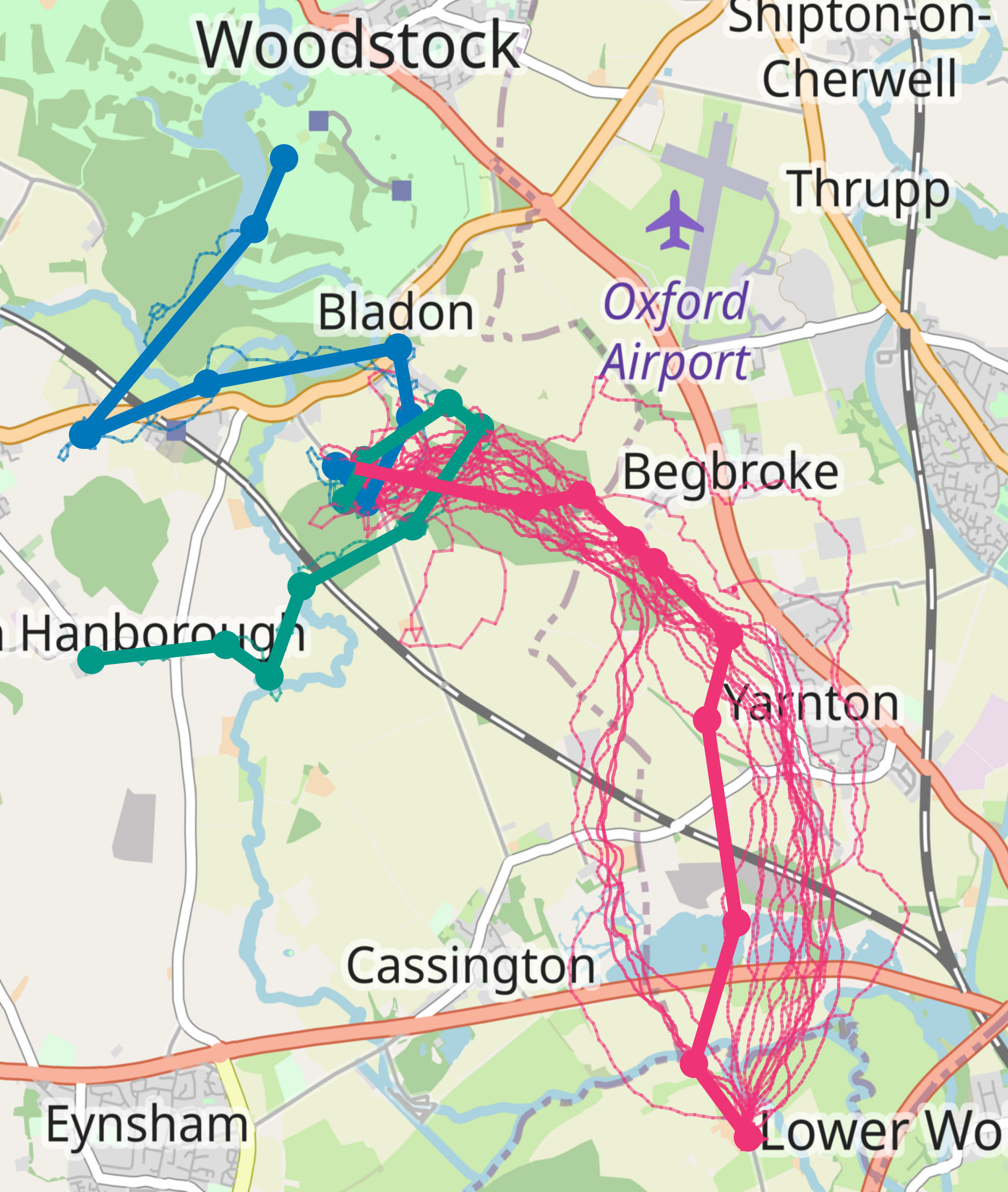
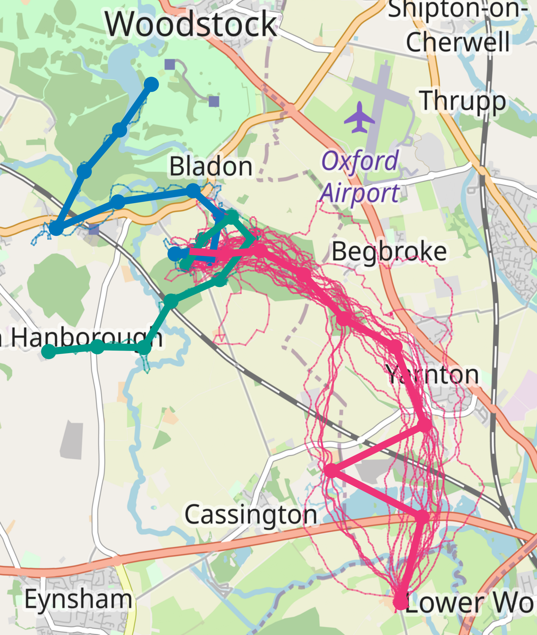
Three subfigures with pigeon trajectories on the map. The trajectories are clustered into three clusters; each cluster has a low-complexity center. The Fréchet distance-based approach and the dynamic time warping-based approach exhibit some artifacts in the cluster centers. Our new approach looks most natural of the three.

Figure 1. Clustering using the Fréchet distance (left), dynamic time warping (middle), and our new approach called continuous dynamic time warping (right), where the color denotes the clusters and the bold trajectories are the cluster centers. While the Fréchet distance shows a strong influence of outliers and dynamic time warping shows discretization issues, clustering via continuous dynamic time warping gives arguably the most natural results. Map data © OpenStreetMap contributors. (OpenStreetMap contributors, 2020)

$(k,\ell)$-Medians Clustering of Trajectories Using
Continuous Dynamic Time Warping

Abstract.

Due to the massively increasing amount of available geospatial data and the need to present it in an understandable way, clustering this data is more important than ever. As clusters might contain a large number of objects, having a representative for each cluster significantly facilitates understanding a clustering. Clustering methods relying on such representatives are called center-based. In this work we consider the problem of center-based clustering of trajectories.

In this setting, the representative of a cluster is again a trajectory. To obtain a compact representation of the clusters and to avoid overfitting, we restrict the complexity of the representative trajectories by a parameter $\ell$. This restriction, however, makes discrete distance measures like dynamic time warping (DTW) less suited.

There is recent work on center-based clustering of trajectories with a continuous distance measure, namely, the Fréchet distance. While the Fréchet distance allows for restriction of the center complexity, it can also be sensitive to outliers, whereas averaging-type distance measures, like DTW, are less so. To obtain a trajectory clustering algorithm that allows restricting center complexity and is more robust to outliers, we propose the usage of a continuous version of DTW as distance measure, which we call continuous dynamic time warping (CDTW). Our contribution is twofold:

1. To combat the lack of practical algorithms for CDTW, we develop an approximation algorithm that computes it.

2. We develop the first clustering algorithm under this distance measure and show a practical way to compute a center from a set of trajectories and subsequently iteratively improve it.

To obtain insights into the results of clustering under CDTW on practical data, we conduct extensive experiments.

1. Introduction

As smartphones have become a ubiquitous part of our daily lives, access to GPS technology has become more convenient than ever. In general, the prevalence of tracking technologies have led to an abundance of GPS data. For example, researchers can track animals in large quantities to help study their behavior, enabling new scientific insights in the field of behavioral biology.

With the blessing of easily available GPS data comes the burden of analyzing large quantities of data, in particular, the need for suitable methods to extract relevant information from the collected data. A classical approach to make large data sets understandable is to cluster the data into different groups. While this makes it easy to identify different groups in the data, it may still be simply too much information to digest or to visualize. Identifying a good representative for each group helps condense the information even further. Clustering methods that rely on such representatives—also called cluster centers—are referred to as center-based clustering.

Let a trajectory be represented by a polygonal chain in Euclidean space. While point sets in Euclidean space have a canonical distance measure (the $L_{2}$-norm), for trajectories there is no such clear choice. Thus, trajectory clustering has been considered under several different distance measures. Two popular distance measures are Dynamic Time Warping (DTW) and the Fréchet distance, but each have their own shortcomings.

Dynamic Time Warping (DTW) matches the vertices from one trajectory to vertices on the other such that the summed distance between matched vertices is minimized. In DTW, only vertices of the trajectory are considered, and the edges between these vertices are ignored. As such, DTW is sensitive to the relative sampling rates of the trajectories and provides a poor matching between a high-complexity trajectory and a low-complexity trajectory. See Figure 2 for an example of this issue. For this reason, DTW is inappropriate for computing low-complexity cluster centers for high-complexity trajectories, as shown in Figure 3.

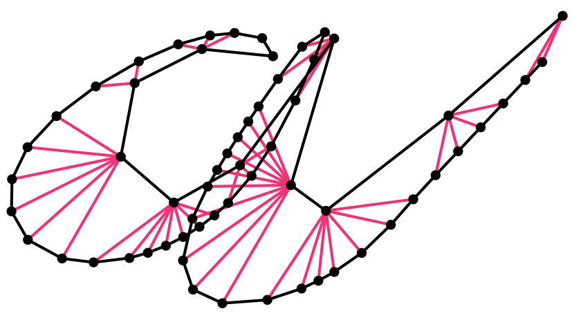
(a) DTW.

(b) CDTW.

Figure 2. An example of discrete and continuous alignments of points along trajectories of differing complexities by DTW and CDTW, respectively.

Two trajectories and the corresponding matchings for DTW and CDTW. The DTW matching looks very unbalanced due to the sampling rate on the two trajectories, unlike the CDTW matching.

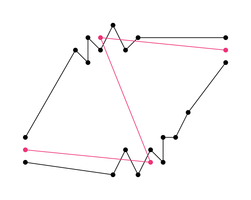
(a) DTW cluster center.

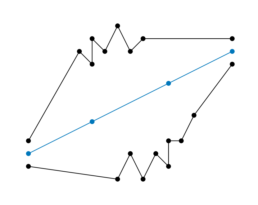
(b) CDTW cluster center.

Figure 3. An example where the low-complexity DTW cluster center is inappropriate for high-complexity trajectories.

Two trajectories and the corresponding low-complexity centers for DTW and CDTW. CDTW center goes smoothly between the trajectories, the DTW center is drawn first to one, then to the other trajectory.

The Fréchet distance captures the minimal cost of a continuous deformation of one trajectory into another, where the cost of deformation is the maximum distance between a point and its transformed counterpart. Recent work on center-based clustering of trajectories has used the Fréchet distance (Buchin et al., 2019a; Buchin et al., 2020; Driemel et al., 2016). The differences of DTW and the Fréchet distance are, first, that the Fréchet distance considers both edges and vertices of the trajectory, and second, that the Fréchet distance is a bottleneck measure (i.e., its cost is a maximum) whereas DTW is a summed measure. As a result of the Fréchet distance being a bottleneck measure, a shortcoming of using the Fréchet distance to compute cluster centers is that it may be sensitive to outliers in the trajectory data. See Figure 4 for an example where this issue occurs.

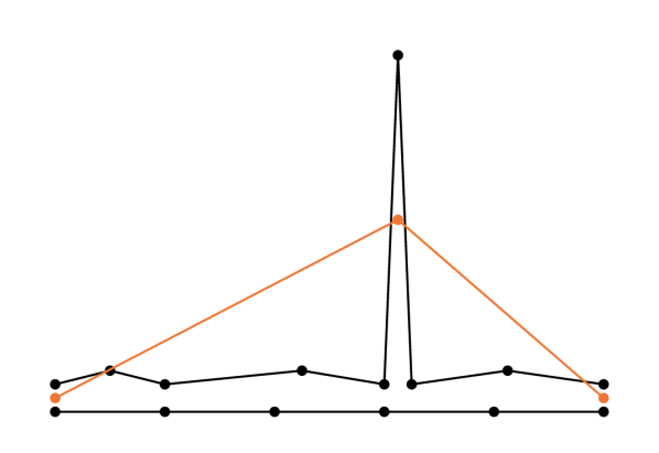
(a) Fréchet cluster center.

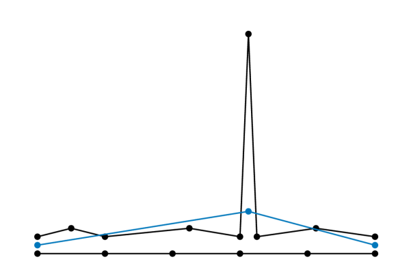
(b) CDTW cluster center.

Figure 4. An example where the quality of the Fréchet cluster center deteriorates in the presence of an outlier.

Two trajectories, one of them with a sharp peak away from the other one in the middle, and the corresponding low-complexity centers for the Fréchet distance and CDTW. The CDTW center is only slightly perturbed at the sharp peak, unlike the Fréchet center.

To overcome the shortcomings of DTW and the Fréchet distance for center-based trajectory clustering, we propose the usage of a continuous version of DTW. We call this measure the continuous dynamic time warping distance (CDTW) and formally define it in Section 3. The advantages of computing cluster centers with CDTW are that it is appropriate for low-complexity centers (see Figure 3) and is robust to outliers (see Figure 4). In Section 6, we provide empirical evidence in support of these claims.

The distance measure we call CDTW was originally introduced as the summed or average Fréchet distance by Buchin (Buchin, 2007, Ch. 6). A different distance measure with the name CDTW was introduced by Munich and Perona (Munich and Perona, 1999). This measure is continuous in the sense that a vertex of a trajectory may be aligned to any point on the other trajectory, instead of only to another vertex. It is, however, still based on discrete summation over the vertices in the same manner as DTW and is therefore still prone to issues regarding sampling of the trajectories. A general definition for a continuous distance measure for trajectories using path integrals with the name CDTW was given by Efrat et al. (Efrat et al., 2007). They also sketch an approximation algorithm for a special case of our definition of CDTW, but it is based on numerical methods for solving eikonal equations, rendering it impractical. A $(1+\varepsilon)$-approximation algorithm for our definition of CDTW was introduced by Maheshwari et al. (Maheshwari et al., 2018). Its running time is upper-bounded by $O(\zeta^{4}n^{4}/\varepsilon^{2})$, where $n$ is the complexity of the trajectories and $\zeta$ is the maximal ratio between the lengths of any pair of segments from the trajectories. This dependency on the ratio between segments makes the algorithm unsuited for the problem of $(k,\ell)$-center based clustering, where one trajectory consists of many short segments and the other of a few long segments. As far as we are aware, there are no exact algorithms known for computing the CDTW distance.

For point sets, clustering algorithms that are parametrized by the number of clusters, like $k$-center or $k$-means clustering, are very common. Trajectories, however, pose the problem that their complexity can vary. Increasing the complexity of the centers also increases the adaptability of the centers to the data at the cost of overfitting and complicated centers. Therefore, recent work introduced the notion of $(k,\ell)$-clustering for trajectories (Buchin et al., 2019a) (and there has been a previous closely related notion for time series (Driemel et al., 2016)), which is a center-based clustering where we require the clustering to have $k$ clusters and each center can have complexity at most $\ell$. More precisely, we consider the following two variants of $(k,\ell)$-clustering:

1. $(k,\ell)$-center clustering: Find $k$ centers of complexity at most $\ell$ that minimize the maximal distance that any trajectory has to its closest center.

2. $(k,\ell)$-medians clustering: Find $k$ centers of complexity at most $\ell$ that minimize the sum of distances of each trajectory to its closest center.

See Section 5 for a formal definition and detailed discussion. Interestingly, different notions of clustering seem more natural for different distance measures. As the Fréchet distance and $(k,\ell)$-center clustering minimize the maximal distance, it seems natural to combine them. Similarly, as DTW / CDTW and $(k,\ell)$-medians minimize a sum / integral, it again seems natural to combine them.

An approximation algorithm for $(k,\ell)$-center clustering using the continuous Fréchet distance was given by Buchin et al. (Buchin et al., 2019a). This algorithm, with additional practical modifications, was later implemented and applied to real-world data by Buchin et al. (Buchin et al., 2019b). For the discrete Fréchet distance, Buchin et al. (Buchin et al., 2020) designed approximation algorithms for $(k,\ell)$-medians clustering and $(k,\ell)$-center clustering. Finally, Petitjean et al. (Petitjean et al., 2011) introduced an algorithm for computing low-complexity centers for a cluster of trajectories using DTW distance.

2. Contributions

Our main contribution is a trajectory clustering implementation using the CDTW distance measure. The advantages of this measure over existing measures are that it is appropriate for low-complexity centers and robust to outliers. To the best of our knowledge, our implementation is the first to cluster trajectories using CDTW. The two main contributions to enable such an implementation are:

• As far as we are aware, there are no exact algorithms for CDTW, and the existing approximation algorithms have a high dependency on both the complexity and the lengths of the input trajectories (Maheshwari et al., 2018). We overcome this obstacle by providing a practically efficient additive approximation algorithm for computing the CDTW distance, and an efficient implementation of said algorithm. See Section 4 for details.

• Again, as far as we are aware, there are no known algorithms for $(k,\ell)$-medians clustering of trajectories under CDTW. We overcome this obstacle by following the method of Buchin et al. (Buchin et al., 2019a). This involves computing an initial $(k,\ell)$-clustering by combining the Gonzalez algorithm or PAM with a trajectory simplification algorithm, and then improving the cluster centers using methods similar to those found in the practical work by Buchin et al. (Buchin et al., 2019b). We explore several methods for improving cluster centers, and perform extensive experiments to compare these methods. See Section 5 for details.

Our experimental results show that our method, which clusters trajectories under the CDTW measure, outperforms similar methods which cluster trajectories under either the Fréchet distance or the DTW measure. The improvement of the CDTW measure over the DTW measure is particularly noticeable for low-complexity cluster centers, and over the Fréchet distance in the presence of outliers. See Section 6 for details.

3. Continuous Dynamic Time Warping

We represent trajectories as polygonal chains, i.e., series of connected line segments. A trajectory $P$ is given by the sequence of its vertices $(p_{1},\dots,p_{n})$, where each $p_{i}\in\mathbb{R}^{d}$ for some $d\geq 1$. The DTW distance and the CDTW distance are summations over distances between aligned points along the trajectories. Among the different possibilities for distance measures between points, we consider the (squared) Euclidean distance to be the most natural choice. Both regular and squared Euclidean distances are commonly used in DTW computation. Furthermore, methods for center computation, such as the least-squares method for linear regression as well as $k$-means clustering, also use the squared Euclidean distance. Thus, in the remainder we also focus on the squared Euclidean distance measure, i.e., the distance between two points $p,q\in\mathbb{R}^{d}$ is defined as $d(p,q)=\left\lVert p-q\right\rVert_{2}^{2}$.

A central definition for the DTW distance is the notion of a discrete warping path. Given a pair of trajectories $P=(p_{1},\dots,p_{n})$ and $Q=(q_{1},\dots,q_{m})$, define $W=(w_{1},\dots,w_{k})$ with $w_{i}\in\{1,\dots,n\}\times\{1,\dots,m\}$. This warping path aligns vertices in $P$ with vertices in $Q$, meaning that $w_{k}=(i,j)$ corresponds to a match of vertex $p_{i}\in P$ to vertex $q_{j}\in Q$. The following restrictions are commonly imposed on discrete warping paths:

1. The first and last vertex in $P$ must be matched to the first and last vertex in $Q$, respectively.

2. Each vertex in $P$ must be matched to at least one vertex in $Q$, and vice versa.

3. The alignment may not move backwards on the trajectories. More precisely, the indices in the warping path must be monotonically increasing, i.e., $i_{k-1}\leq i_{k}$ and $j_{k-1}\leq j_{k}$.

Note that from (2) and (3) it follows that the warping path can only step to neighboring vertices. For DTW, the cost of a warping path is the sum of distances between aligned vertices. The DTW distance $\delta_{D}(P,Q)$ between a pair of trajectories is then the value of the minimal-cost warping path:

$$\delta_{D}(P,Q)\coloneqq\min_{W}\sum_{(i,j)\in W}d(p_{i},q_{j})\,.$$

Let $L(P)$ denote the total arc length of a trajectory $P$. We define the parameter space $\mathbb{P}=[0,L(P)]\times[0,L(Q)]$ as an axis-aligned rectangle representing all pairs of points in trajectories $P$ and $Q$. Let $P(t)$ denote the point that lies arc length $t$ along $P$. Then, each $(p,q)\in\mathbb{P}$ corresponds to a pair of points $(P(p),Q(q))$. We define a height function $h\colon\mathbb{P}\to\mathbb{R}^{+}$ over the parameter space that gives the distance between the corresponding points, i.e., $h((p,q))\coloneqq d(P(p),Q(q))$. Figure 5 shows an example of the parameter space and height function for the pair of trajectories in Figure 2.

A continuous warping path $\pi\colon[0,1]\to\mathbb{P}$ aligns points in $P$ to points in $Q$, i.e., if $(p,q)$ is in the image of $\pi$, the point $P(p)$ is aligned to the point $Q(q)$. We impose restrictions on continuous warping paths similar to those for its discrete counterpart.

1. The first and last vertex in $P$ must be matched to the first and last vertex in $Q$, respectively.

2. Every point in $P$ must be matched with at least one point in $Q$, and vice versa.

3. The alignment may not move backwards over the trajectories. More precisely, both coordinates of $\pi$ must be monotonically increasing.

It follows that $\pi$ is a continuous function that monotonically increases from $\pi(0)=(0,0)$ to $\pi(1)=(L(P),L(Q))$. For CDTW, the cost of a warping path is the integral over distances between aligned points. Therefore, a natural definition is the path integral over $\pi$ through $h$:

$$\int_{\pi}h(r)\,\mathrm{d}r=\int_{0}^{1}h(\pi(t))\cdot\left\lVert\pi^{\prime}(t)\right\rVert\,\mathrm{d}t\,.$$

It may be desirable to use different norms for the speed of the path $\left\lVert\pi^{\prime}(t)\right\rVert$, so we generalize the definition to support this. The CDTW distance between a pair of trajectories using the $L_{p}$-norm in parameter space is the cost of the continuous warping path with minimal cost:

$$\delta^{p}_{CD}(P,Q)\coloneqq\min_{\pi}\int_{0}^{1}h(\pi(t))\cdot\left\lVert\pi^{\prime}(t)\right\rVert_{p}\,\mathrm{d}t\,.$$

By using $p=1$, the path length $\int_{0}^{1}\left\lVert\pi^{\prime}(t)\right\rVert_{1}\,\mathrm{d}t=L(P)+L(Q)$ is the same for all warping paths, as noted by Buchin (Buchin, 2007), thus allowing for normalization and easier comparison. In a similar setting, $p=\infty$ was used to place a speed limit on the warping path (Rote, 2014). We identify $p=1$ and $p=\infty$ as good choices for $p$, in particular due to their natural meaning as the sum and the maximum of speeds along the trajectories. In this work we use $p=1$ and thus define $\delta_{CD}(P,Q)\coloneqq\delta^{1}_{CD}(P,Q)$. An example of minimal-cost warping paths for both DTW and CDTW is shown in Figure 5.

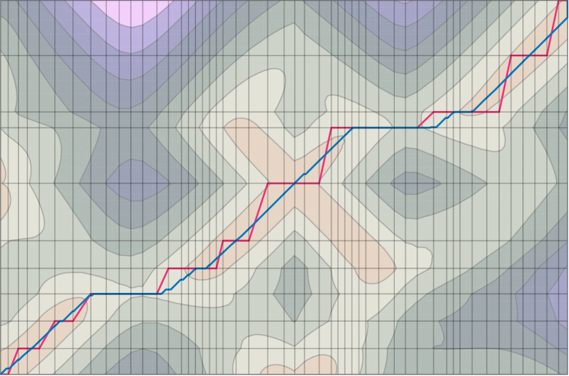
A figure showing the parameter space with a color map for matchings of higher and lower cost and two warping paths. The one for DTW goes from vertex to vertex, so horizontally, vertically, or diagonally. The one for CDTW can cross the grid lines in the parameter space at any point.

Figure 5. Warping paths of DTW and CDTW through parameter space corresponding to the trajectories in Figure 2. The grid lines correspond to the vertices of the trajectories.

4. Computing CDTW

The task of computing the continuous dynamic time warping distance reduces to finding an optimal warping path, i.e., a warping path for which the CDTW cost is minimized. We first split the problem into smaller subproblems which can easily be solved exactly, and then apply existing algorithms to combine the exact solutions into an approximation of an optimal warping path.

As follows from the description in Section 3, the segments of the trajectories induce a grid of axis-aligned rectangular cells over the entire parameter space, such that each cell uniquely corresponds to a pair of segments. See Figure 5 for an example of such a parameter space with its grid of cells. The height function over a single cell is therefore a function over linear interpolations of the segments. More precisely, we define the height function at the point $(p,q)\in\mathbb{P}$ in a parameter space cell as

$$h((p,q))\coloneqq(p-a)^{2}+(q-b)^{2}+2\lambda(p-a)(q-b)+c\,,$$

where the values for $a,b\in\mathbb{R}$ are based on the offset of the cell’s corresponding segments along the infinite lines on which they lie. Note that these values are fixed for each cell. The value of $-1\leq\lambda\leq 1$ is the dot product between the unit direction vectors of the segments and is fixed for each cell as well. The value of $c$ is the smallest distance between the infinite lines of the segments and is therefore non-zero only in the degenerate case of parallel lines. The level sets of the height function $h$ form concentric ellipses with center $(a,b)$ and eccentricity based on $\lambda$, possibly degenerating into parallel strips. Let $\ell_{m}$ be the line through the point $(a,b)$ with slope $1$, coinciding with the $xy$-monotone axes of the ellipses. Figure 6 shows a number of these level sets and the $\ell_{m}$ line.

Given a cell $C$ and points $s,t\in C$ with $s_{x}\leq t_{x}$ and $s_{y}\leq t_{y}$ and assuming without loss of generality that $s$ and $t$ are the bottom left and top right corners of $C$, respectively, we can compute the optimal warping path from $s$ to $t$ as shown by Maheshwari et al. (Maheshwari et al., 2018):

• If $\ell_{m}$ intersects the border of $C$, let $c_{s}$ and $c_{t}$ be the points of intersection closest to $s$ and $t$, respectively. Then the optimal warping path is $(s,c_{s},c_{t},t)$.

• Otherwise, let $c$ be the corner point closest to $\ell_{m}$. Then the optimal warping path is $(s,c,t)$.

An example for both cases is shown in Figure 6. Note that in both cases the optimal warping path consists of a constant number of linear pieces. We integrate along each linear piece to compute the cost of the warping path from $s$ to $t$.

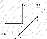
Two paths within a cell, depending on the starting and ending location. One follows the cell border, then the line $l_{m}$, then another cell border; the other does not reach $l_{m}$, so just follows the two borders.

Figure 6. Two types of optimal warping paths through a single cell: $(s,c_{s},c_{t},t)$ via $\ell_{m}$, and $(s^{\prime},c^{\prime},t^{\prime})$ missing $\ell_{m}$.

With this algorithm for computing the optimal warping path through single cells, it remains to find the points where the optimal warping path crosses from one cell to another. To this end, define a graph over the parameter space. Take the corner points of the cells as the vertices of the graph. To improve the accuracy of the warping path, we uniformly sample additional vertices (called Steiner points) along the borders of each cell, such that the distance between two neighboring sampled vertices is at most $\Delta$ in the original Euclidean space. We add an edge between two vertices $s$ and $t$ if both vertices lie in the same cell and are positioned such that $s_{x}\leq t_{x}$ and $s_{y}\leq t_{y}$. Each edge is assigned a weight equal to the cost of the optimal warping path between its incident vertices. An example of vertex placement and edges is shown in Figure 7. The cost of the shortest path through this graph from $(0,0)$ to $(L(P),L(Q))$ is an additive approximation to the cost of the optimal warping path.

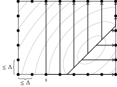
The cell with regularly sampled entry and exit points on the borders. Depending on the level sets and the choice of points, the path through the cell may differ.

Figure 7. Example placement of vertices along the borders of a cell, and an example of the edges originating from one such vertex $s$ visualized by the optimal warping paths.

Any algorithm that finds the shortest path between two given vertices in an acyclic graph with positive edge weights will be sufficient in finding the approximation of the optimal warping path. In our implementation we use bidirectional Dijkstra’s algorithm as it often needs to consider fewer vertices than regular Dijkstra’s algorithm. This algorithm searches from both the start and goal vertex until the two search fronts meet with an appropriate stopping condition. In practice we do not compute the entire graph in advance; instead, for a given vertex, we compute the adjacent vertices and incident edges on the fly as they are explored by the shortest path algorithm.

5. Clustering Algorithms

Before we present our clustering algorithms, we first formally define the two notions of clustering that were presented in Section 1. Let $\mathcal{C}$ be a set of trajectories and let $k$ and $\ell$ be positive integers. Let $d$ be some distance measure for trajectories. In a $(k,\ell)$-clustering problem, we seek to compute a set of $k$ center trajectories $\mathcal{Q}$ of complexity at most $\ell$ which is optimal according to some cost function. The two notions we consider are:

1. In $(k,\ell)$-center clustering, the maximum distance from each trajectory in $\mathcal{C}$ to the nearest center in $\mathcal{Q}$ is minimized, i.e., the relevant cost function is

   $$\phi_{\infty}(Q)\coloneqq\max_{C\in\mathcal{C}}d(C,\mathcal{Q})\,.$$

2. In $(k,\ell)$-medians clustering, the sum of distances from each trajectory in $\mathcal{C}$ to the nearest center in $\mathcal{Q}$ is minimized, i.e., the relevant cost function is

   $$\phi_{1}(Q)\coloneqq\sum_{C\in\mathcal{C}}d(C,\mathcal{Q})\,.$$

For some variants we also consider $(k,\ell)$-medians clustering where we use the squared $L_{2}$-norm as the underlying distance measure. This can also be considered a means clustering.

Our high-level strategy for $(k,\ell)$-medians clustering is as follows. We first compute an initial set of $k$ centers, each of them being an $\ell$-simplification of a trajectory from the input set. We then apply an iterative center improvement algorithm to obtain cluster centers that are not restricted to the vertices of the input trajectories.

5.1. Computing the Initial Clustering

We use the partitioning around medoids (PAM) method, also called $k$-medoids, proposed by Kaufman and Rousseeuw Kaufman and Rousseeuw, 1987, Kaufman and Rousseeuw, 1990, Ch. 2 and recently improved by Schubert and Rousseeuw (Schubert and Rousseeuw, 2019). However, we adapt the method to the $(k,\ell)$-medians clustering setting. The PAM method for $k$-medians clustering in general metric spaces works by first greedily choosing an initial set of centers. In this step, we compute the reduction in the sum of distances from trajectories to cluster centers for each trajectory and then choose the one that gives the biggest reduction as a new center; we add $k$ centers this way. Next, the algorithm enters a local search phase where for each center $c_{i}$, we evaluate the possible reduction in the sum of distances if we swap $c_{i}$ for a non-center $x$. We perform the swap that gives the biggest difference and repeat the procedure iteratively until we find a local optimum. Adapting this approach to our setting is straightforward. Whenever we consider a trajectory as a center, we compute the distances to its $\ell$-simplification.

We also adapt the greedy algorithm of Gonzalez to the setting of $(k,\ell)$-clustering (Gonzalez, 1985). The idea is simple: we start with a random input trajectory as the first center; then we iteratively pick the trajectory which is furthest from the already picked centers until we get $k$ centers. The only difference is that we pick the $\ell$-simplifications of the center trajectories, and compute the distances accordingly. Even though the Gonzalez algorithm optimizes for the $k$-center cost function, it is known to be a $2n$-approximation for the $k$-medians problem, where $n$ is the number of input points (Har-Peled, 2011, Ch. 4). Therefore, we use the Gonzalez algorithm as a baseline for our initial clustering approaches. We also consider an alternative clustering algorithm that first computes a $(k,\ell)$-clustering using the Gonzalez algorithm and then applies the local search of PAM.

5.2. Trajectory Simplification

To use the approach described in Section 5.1, we need to compute the $\ell$-simplifications of the center trajectories when computing an initial clustering. The choice of simplification approach to use is somewhat independent of the clustering methods: we need to choose an approach that allows us to restrict the maximum complexity of the simplified trajectory to $\ell$ and gives good simplifications, both visually and in terms of CDTW. As this is only used as the initial step before improving the centers, we choose the simpler approach of vertex-restricted simplification, where the vertices of the simplified trajectory are a subset of the vertices of the original trajectory. We focus on two simplification methods: the dynamic programming approach suggested by Imai and Iri (Imai and Iri, 1988) and the greedy approach by Agarwal et al. (Agarwal et al., 2005).

The greedy approach is very efficient, offers reasonable guarantees for the Fréchet distance, and works well in practice. The main idea is: given a threshold and a starting vertex of the trajectory $p_{i}$, go along the trajectory until we reach a vertex $p_{j}$ such that the distance of choice between the segment $p_{i}p_{j+1}$ and the subtrajectory from $p_{i}$ to $p_{j+1}$ exceeds the threshold. Here $i$ and $j$ are indices of vertices of the trajectory with $j>i$. Once that happens, we add the segment $p_{i}p_{j}$ to our simplification and set the vertex $p_{j}$ as the next starting point. We repeat the process until we reach the end of the trajectory. This method can be used to obtain a simplification of complexity $\ell$ by performing a binary search on the threshold value.

The Imai–Iri approach allows to compute an optimal simplification in a local sense, i.e., assuming the matching is fixed at the points that coincide between the trajectory and its simplification. There are two reasonable approaches to its implementation:

1. Given a threshold, save all the possible line segments between vertices of the trajectory for which the distance to the corresponding subtrajectory is below the threshold. Then find the shortest path from the beginning to the end of the trajectory. This can be adapted to targeting the specific $\ell$ using binary search on the threshold value.

2. Given a target $\ell$, use a dynamic program to record the costs of all possible shortcuts in $\ell$ steps and find the lowest-cost solution. This approach seems more suitable for sum-based distances like DTW and CDTW.

It is not obvious which approach would be preferable in our setting, since any of these could be used with DTW, the Fréchet distance, and CDTW. We conduct an experimental evaluation and describe the results in Section 6.3. Based on these results, we choose the greedy approach with Fréchet distance in all our clustering pipelines.

5.3. Improving Cluster Centers

Petitjean et al. (Petitjean et al., 2011) introduced a method called DTW Baricenter Averaging (DBA) to improve the centers in $k$-means clustering using the DTW distance. Let $\mathcal{C}$ be a trajectory cluster and let $C=(c_{1},\dots,c_{l})$ be its initial center. The DBA method first computes the DTW matching between the center $C$ and all trajectories in the cluster $\mathcal{C}$. For all $1\leq i\leq l$, let $\tilde{c_{i}}$ be the average of all points matched to $c_{i}$. We replace the initial center $C$ with the new center $\tilde{C}=(\tilde{c_{1}},\dots,\tilde{c_{l}})$ if it induces a lower cost. The procedure is repeated until the new center does not improve upon the current center.

We use a similar method to improve the cluster centers arising from the CDTW distance. We call our method CDTW Barycenter Averaging (CDBA). A key difference between the DBA method and our CDBA method is that ours uses a continuous matching, so a vertex on $C$ may be mapped to an entire subtrajectory rather than a set of vertices. In this situation, we uniformly sample points on the matched subtrajectory. The number of sampled points is proportional to the ratio of the length of the subtrajectory to the length of the trajectory. See Figure 8 for an example where the matching is sampled to compute the updated centers.

The sampling method for vertices mapped to a continuous subtrajectory has been previously used by Buchin et al. (Buchin et al., 2019b). Their work focuses on $(k,\ell)$-center clustering using the Fréchet distance, and we refer to their method as free space averaging (FSA). In the FSA method, rather than updating vertices of the center trajectory to be the mean of the points they are matched to, vertices are assigned to the center of the minimum enclosing circle of the points they are matched to in the Fréchet matching.

The intuition behind the center update methods described above is that by moving vertices of the center trajectory closer to the points on cluster trajectories to which they are aligned with respect to the distance measure under consideration, we expect the new center trajectory to be a better fit for the cluster. This intuition makes the implicit assumption that the alignment between the center trajectory and trajectories in the cluster does not change too much after the update. The update method for each distance function also depends on the type of clustering considered to be most natural for that particular distance function. The Fréchet distance minimizes the maximum distance between aligned points. Similarly, $k$-center clustering minimizes the maximum distance between each trajectory and the trajectories in the associated cluster, and so $k$-center clustering seems a natural choice for clustering with the Fréchet distance. The FSA method described was designed by Buchin et al. (Buchin et al., 2019b) for the purpose of improving centers in $(k,l)$-center clustering. Both DTW and CDTW are distance measures that minimize the sum or integral of distances between aligned points. Therefore, $k$-means or $k$-medians clustering seem to be more natural choices for these distance measures. The DBA center update method we have described was designed by Petitjean et al. (Petitjean et al., 2011) in the context of $k$-means clustering under the DTW distance measure, while we apply the CDBA method for $k$-medians clustering under CDTW.

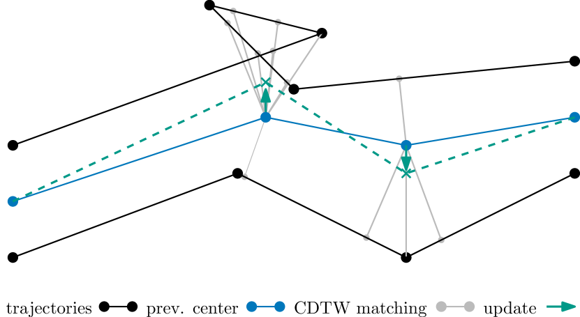
Two trajectories and the center. The vertices of the center are matched to subtrajectories. We sample those subtrajectories, thus pulling the vertices of the center more strongly in the direction where there are more samples.

Figure 8. The CDBA update method, with the CDTW matching sampled uniformly to compute the updated centers.

The CDBA method is based on the strategy of moving vertices. However, the definition of CDTW also takes into consideration the internal points on edges. Therefore, we also consider a center update method which aims to optimize the position of edges, rather than just vertices. With this in mind, we introduce an alternative center update method for $(k,\ell)$-medians clustering under CDBA which we call the wedge method. Given an initial center trajectory $C=(c_{1},c_{2},\dots,c_{\ell})$ and the associated cluster $\mathcal{C}$, the wedge method works as follows. For each $c_{i}$, $1<i<\ell$, we define the line segments $s_{L}=c_{i-1}c_{i}$ and $s_{R}=c_{i}c_{i+1}$. We then define the sets $L$ and $R$ to be all vertices of trajectories in $\mathcal{C}$ aligned by CDTW to $s_{L}$ and $s_{R}$, respectively. For each vertex $p$ of a trajectory $P\in\mathcal{C}$ aligned to either $s_{L}$ or $s_{R}$ under CDTW, we define $w(p)$ to be the sum of lengths of the segments preceding and following $p$ on $P$. We search for a point $\tilde{c_{i}}$ by perturbing $c_{i}$ so as to minimize

$$\sum_{p\in L}w(p)\cdot\gamma(p,c_{i-1}\tilde{c_{i}})^{2}+\sum_{p\in R}w(p)\cdot\gamma(p,\tilde{c_{i}}c_{i+1})^{2}\,,$$

where $\gamma(p,s)$ denotes the distance from a point $p$ to the closest point on a line segment $s$.

Finally, we can perform a similar optimization for the first and last points on the initial center trajectory. Depending on the nature of the data we are working on, it may make more sense to keep the start and end points fixed, as is the case in the data set of pigeon flight paths we study. We include the weight terms $w(\cdot)$ as we expect vertices between longer segments to contribute more to the value of the CDTW distance.

6. Experiments

In this section, we describe the experiments performed on the methods described above and their results.

6.1. Data Sets

We have conducted experiments on three different open-source real-world data sets. The first of these is a set of handwritten characters of the English alphabet (Williams, 2008) from the UCI Machine Learning Repository (Dua and Graff, 2017). The data set contains a few hundred examples in each of twenty classes, with each class corresponding to a character that can written in a single stroke.

We also make use of the pigeon flight path trajectory data set by Mann et al. (Mann et al., 2010). The data set consists of flight paths of pigeons released from four distinct release sites as they fly to a common return site. For each release site, the data set contains trajectories corresponding to seven or eight distinct pigeons, each of which is released approximately twenty times.

Finally, we also make use of the stork migration data by Rotics et al. (Rotics et al., 2018b), made available at the Movebank data repository (Rotics et al., 2018a). The data set contains the movements of 35 adult storks over four years as they migrate from Africa to Europe.

As our methods become impractical for very large trajectories (some trajectories in the stork migration data set contain over 15000 points), we pre-process the data by regularly sampling points to ensure the trajectories we use have at most a few hundred vertices. The coordinates in the pigeon and stork data sets are given as latitude and longitude. Since our methods assume trajectories in the plane, we apply projections to the data sets. We use the transverse Mercator projection for the pigeon data set and the two-point equidistant projection for the stork data set.

We conduct experiments to evaluate the three steps in our trajectory clustering implementation, that is, our initial clustering, our trajectory simplification, and our center improvement methods. We compare our results to existing approaches. In particular, we compare the quality of trajectory simplifications based on DTW and the Fréchet distance with our algorithm based on CDTW, and we compare the quality of center improvement methods based on DBA and FSA with our CDBA and wedge methods. We make the source code of our C++ implementation publicly available.

6.2. Initial Clustering

We apply the PAM clustering algorithm to the pigeon flight data. For each of the four release sites, we compute $(k,\ell)$-clusterings, for $k\in\{1,\dots,7\}$ and $\ell=10$, using the following algorithms with CDTW and greedy simplification with the Fréchet distance:

1. The Gonzalez algorithm;

2. PAM after initializing the centers using the Gonzalez algorithm;

3. PAM after greedily initializing the centers according to the $\phi_{1}$ cost function.

Since the Gonzalez algorithm is randomized, when clustering via algorithms (1) and (2), we take the best of five iterations as the final result. To compare the approaches, we evaluate the values of the $(k,\ell)$-medians scores for the resulting clusterings. Both PAM and PAM with Gonzalez initialization consistently outperform the vanilla Gonzalez approach. This is to be expected, since the Gonzalez algorithm does not aim to optimize the $(k,\ell)$-medians score. The results also indicate that PAM and PAM with Gonzalez initialization often arrive at the same final clustering.

6.3. Trajectory Simplification

As described in Section 5.2, there are many possible approaches to trajectory simplification in our setting. We focus on the greedy approach and the dynamic programming approach, using DTW, the Fréchet distance, and CDTW. We experimentally evaluate these approaches to gauge their performance both visually and with respect to CDTW. In order to do that, we sample trajectories from two of the data sets we use, the character and the pigeon data set. We additionally subsample each trajectory at regular intervals to get trajectories of complexity 50. We then use the different methods to simplify the trajectories to complexity 12 and evaluate the resulting simplifications with respect to CDTW to the original trajectories. The results are shown in Tables 1 and 2.

Table 1. Simplification methods on the characters data set. Reported values are computed over the data set w.r.t. CDTW between the trajectories and their simplifications.

		mean	min	max
DTW	Greedy	255.5	1.90	2001.0
	Imai–Iri	175.6	1.58	1827.4
Fréchet	Greedy	71.4	0.88	695.2
	Imai–Iri	67.4	0.69	689.5
CDTW	Greedy	68.2	0.93	665.5
	Imai–Iri	36.9	0.47	469.1

Table 2. Simplification methods on the pigeons data set (the Bladon Heath site). Reported values are computed over the data set w.r.t. CDTW between the trajectories and their simplifications.

		mean	min	max
DTW	Greedy	0.829	0.003	9.87
	Imai–Iri	0.586	0.005	4.68
Fréchet	Greedy	0.879	0.024	10.19
	Imai–Iri	0.676	0.023	6.60
CDTW	Greedy	0.883	0.008	9.14
	Imai–Iri	0.335	0.005	3.87

As can be seen from the tables, using CDTW with Imai–Iri gives the best results, as expected. Unfortunately, this is also the slowest method, several orders of magnitude slower in our experiments than approaches that use the Fréchet distance or DTW, which makes it impractical. Using the greedy approach with CDTW gives simplifications of only slightly worse quality (see Figure 9), but still shows high computation times.

Other contenders show comparable (amongst each other) results on the two data sets, as can be seen from the results in both tables. They are also all much faster; so, it makes sense to examine the specific defects that arise from each approach to better understand which methods are more suitable in our setting. On the characters data set, DTW fares poorly both using Imai–Iri and the greedy approach. Figure 9 showcases a bad example for dynamic time warping with the Imai–Iri approach, compared to the performance of Imai–Iri with CDTW on the same trajectory. Due to the discrete nature of DTW, points have to be placed somewhat regularly, including on straight-line parts of the trajectory. Since $\ell$ is fixed, DTW-based approaches visually perform poorly on the curved parts. This is reflected in the values of CDTW. Even though DTW performs better on (part of) the pigeon data set, using it in general settings is not ideal, since there are many real-world trajectories with both long straight segments and smooth curvature that will yield bad results, e.g., plane or road vehicle trajectories.

Approaches based on the Fréchet distance fare much better on the character data set and comparably on the pigeons data set. Visual representations of the worst examples compared to Imai–Iri CDTW are shown in Figure 10. Note that here the issue is simply the lack of attention for long segments that do not quite coincide with the trajectory, something that is cost-free for the Fréchet distance, but penalized quite heavily for CDTW. Fréchet-induced simplifications, however, do concentrate the points in the curved sections of the input instead of the straight-line segments, and tend to use less points than the available number $\ell$. Note that we use the simplifications of the center trajectories only as a starting point in our clustering approach before doing further center improvements. Our center improvement strategies can add points in the places that benefit most from it, thus alleviating some of the issues with the Fréchet simplifications. So, Fréchet distance-based simplifications seem to be a good fit for our clustering approach, assuming we cannot use CDTW-based simplification due to the high running time. The greedy approach using the Fréchet distance is very fast, on par with DTW computations, so using it on the fly is feasible. Therefore, in our clustering approach we use the greedy approach with the Fréchet distance to compute the $\ell$-simplifications.

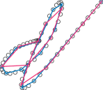
(a) Imai–Iri approach with dynamic time warping.

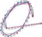
(b) The greedy approach with CDTW.

Figure 9. Example simplifications for DTW and CDTW. Over the original trajectory, two simplifications are shown in color. Imai–Iri approach with CDTW performs best.

Letters ‘l’ and ‘o’, handwritten, and the simplifications. The Imai–Iri approach with DTW misses curved parts. The greedy approach with CDTW is good, although uses the placement of points less nicely than Imai–Iri with CDTW.

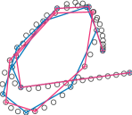
(a) The greedy approach with the Fréchet distance.

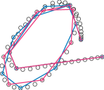
(b) Imai–Iri approach with the Fréchet distance.

Figure 10. Example simplifications for the Fréchet distance. Over the original trajectory, two simplifications are shown in color. Imai–Iri approach with CDTW performs best.

Letter ‘o’, handwritten, and the simplifications. Both approaches with the Fréchet distance deviate somewhat on the long segments, but perform surprisingly well.

6.4. Improving Cluster Centers

We conduct experiments to evaluate the quality of the DBA, FSA, CDBA, and wedge methods for improving cluster centers. First, we conduct an experiment using the character data set to compare the quality of the centers produced according to the CDTW $(k,\ell)$-medians cost. In particular, since our CDBA and wedge methods are designed to minimize the CDTW $(k,\ell)$-medians cost, we expect them to outperform DBA and FSA. The experiment is conducted as follows. For each character, we sample fifty trajectories from the data. For each of these sets of fifty trajectories, we compute an initial $(k,\ell)$-medians clustering, for a fixed $k$ and a range of values for $\ell$, using our version of the PAM method with CDTW and greedy simplification with the Fréchet distance. We then apply four different center improvement algorithms to the same initial clustering. Each method iteratively updates the center trajectory until the method does not make an improvement or until we reach twenty iterations.

We manually select the values of $k$ and $\ell$ that reasonably reflect the underlying trajectories in the data set. For the characters data set, there seems no inherently correct value for $k$, so we choose $k=2$ to accommodate for possible deviations in handwriting. Furthermore, we choose $\ell\in\{6,9,12\}$, as the shape of the characters can be represented by trajectories of this complexity. Note that the general problem of parameter selection is a difficult one. Reddy and Vinzamuri (Reddy and Vinzamuri, 2014) discuss common ways to choose $k$. The general model selection techniques suitable for picking $k$ (e.g., information criteria) can also be applied to choose $\ell$. These methods are especially preferred for data sets where the true complexities of the underlying trajectories are difficult to estimate.

The results of the experiments for $k=2$ and $\ell\in\{6,9,12\}$ are shown in Figure 11. On the $y$-axis are the average CDTW $(k,\ell)$-medians scores over the twenty characters in the data sets. The FSA method obtains significantly higher $(k,\ell)$-medians scores for all values of $\ell$. The DBA method obtains lower $(k,\ell)$-medians scores than FSA, but the score degrades more quickly when the complexity of the cluster center decreases. This supports our claim in the introduction that clustering based on DTW is sensitive to low-complexity cluster centers.

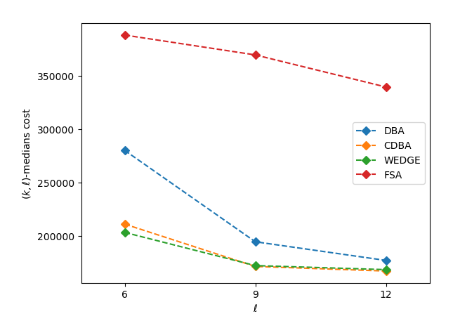
A line plot with $k=6,9,12$ on the $x$-axis and the cost on the $y$-axis. The FSA line is high above the rest. The wedge method is only slightly better than CDBA. DBA is comparable to both for $k=12$, but becomes much worse for $k=6$.

Figure 11. A comparison of the average $(k,\ell)$-medians score over the twenty characters, for different values of $\ell$.

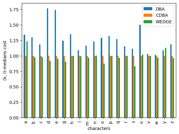
A column plot per character. CDBA cost is scaled to $1$; the wedge cost is mostly a bit lower, the DBA cost is mostly a bit higher, with quite a few columns where it is significantly higher.

Figure 12. Comparison of improvement methods on handwritten character data set with $k=2$, $\ell=6$.

Next, we plot the CDTW $(k,\ell)$-medians cost of the twenty character classes in Figure 12. We do so for $k=2$ and $\ell=6$. The costs for FSA are significantly higher than the other three methods so we omit the FSA results from the plots. As expected, the CDBA and wedge methods outperform DBA on the CDTW $(k,\ell)$-medians cost on all characters. We select a few examples to highlight why we believe this is the case. In particular, we show that there are apparent visual artifacts in clusterings where DBA and FSA obtain a significantly higher $(k,\ell)$-medians cost.

In Figure 13 in the appendix, FSA obtains a significantly higher $(k,\ell)$-medians cost than DBA, CDBA and the wedge method. The green center computed by FSA is significantly distorted while the CDBA and DBA centers are more consistent with the data. In Figure 14 in the appendix, DBA obtains a significantly higher $(k,\ell)$-medians cost than CDBA and the wedge method. The purple center trajectory computed by DBA seems “collapsed” compared to the centers computed by CDBA and the wedge method. These visual artifacts are similar to those shown in Figures 3 and 4.

We perform similar experiments for the pigeons data set and the storks migration data set. For both data sets we selected $k=3$. For the pigeon data we used $\ell=10$, while for the stork data we used $\ell=14$. The $(k,\ell)$-medians costs for FSA and DBA were significantly higher than those for CDBA and the wedge method, but figures for these were omitted due to space constraints. We focus on highlighting the visual artifacts in the clustering that we believe cause FSA and DBA to obtain these significant costs. In Figure 15 in the appendix, the artifacts of DBA are again clearly visible. The blue center produced by FSA seems to zigzag more than the centers produced by CDBA and the wedge method. The CDTW-based center improvement methods appear to give the smoothest and most natural blue center trajectories in these examples. In Figure 16 in the appendix, the blue centers produced by the CDBA and wedge methods are smoother and a better fit for the data than the center produced by DBA. The center trajectories produced by FSA bypass a sharp turn which appears to be a key feature of the data set. The CDBA and wedge methods nicely capture this feature.

Because of the visual artifacts in the characters, pigeons, and stork migration data sets, we are inclined to believe that CDBA and the wedge method produce superior cluster centers. For the same reason, we believe that the $(k,\ell)$-medians cost is a reasonable measure to evaluate clustering algorithms, as it produces high costs on visually unintuitive cluster centers.

7. Conclusions

In this work we presented the first Continuous Dynamic Time Warping (CDTW) implementation that we know of. One reason why we are interested in a practical implementation of this distance measure is enabling a center-based clustering approach that neither requires high-complexity representatives nor is sensitive to outliers. We conducted extensive experiments to evaluate our approach.

Our findings are that we should use the PAM method (partitioning around medoids) alongside the Gonzalez algorithm for initializing the centers. To compute an $\ell$-simplification of the initial centers, the Imai–Iri approach using CDTW gives the best results, but the greedy approach using the Fréchet distance gives the best running time performance. We provided two novel methods of updating the initial cluster centers using the CDTW measure. Our CDTW-based update method avoids many of the artifacts that appear in DTW- or Fréchet-based update methods, especially in the presence of outliers or low-complexity centers.

Interesting future work includes finding algorithmic approaches that lead to faster running times for CDTW computations and extending the usage of this distance measure to fields where DTW is currently predominantly used.

Appendix A Additional Figures

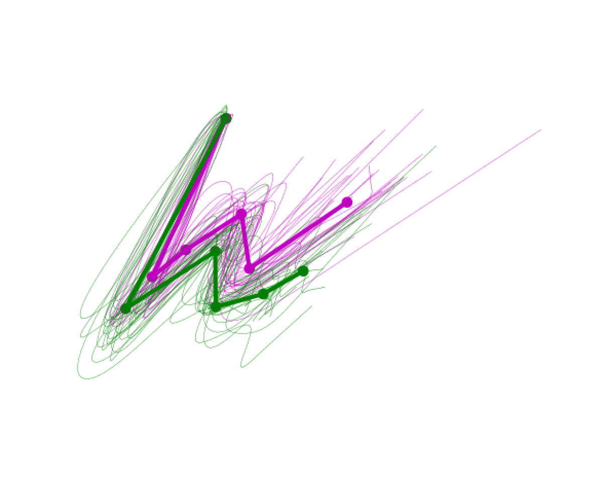
(a) DBA.

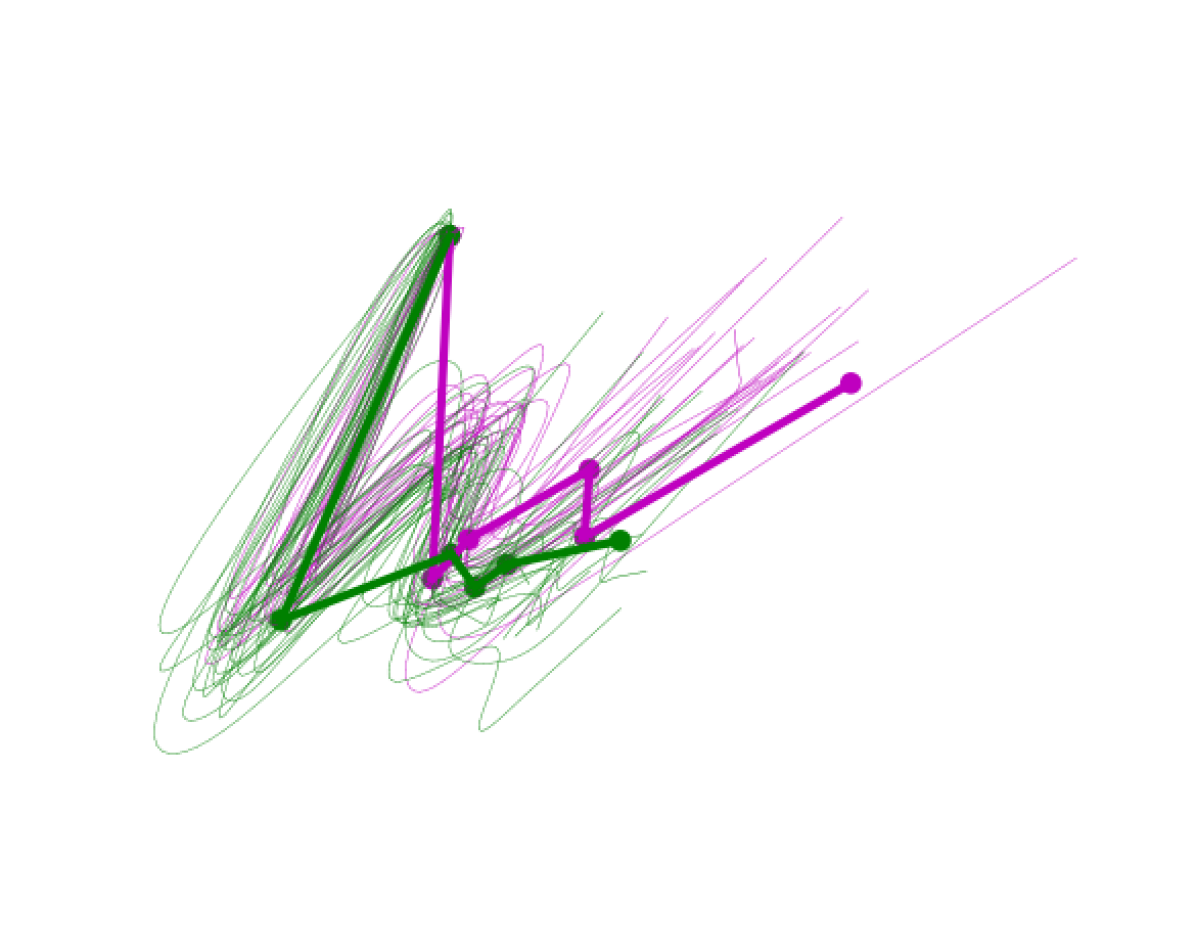
(b) FSA.

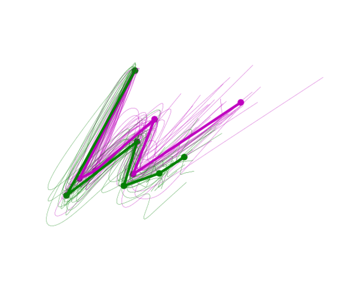
(c) CDBA.

Figure 13. (2, 6)-clusterings of h characters computed with DBA, FSA and CDBA.

Two clusters for character ‘h’. The DBA and CDBA cluster centers look like an ‘h’, the FSA cluster centers have the second part of ‘h’ barely pronounced.

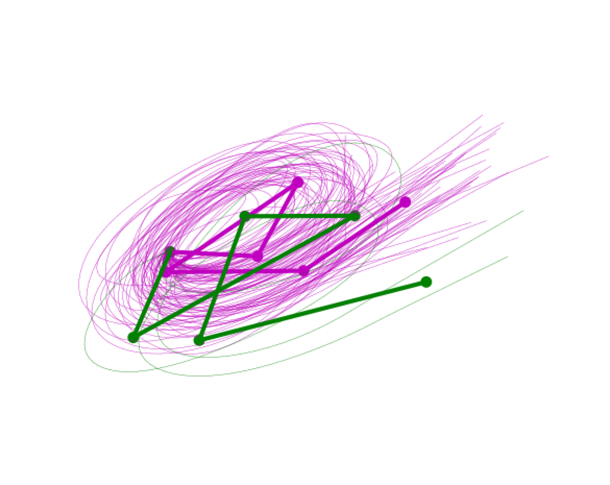
(a) DBA.

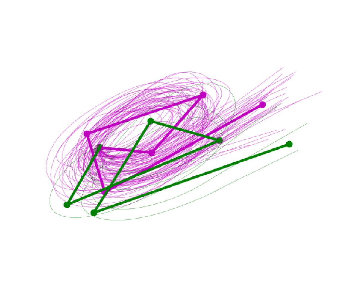
(b) CDBA.

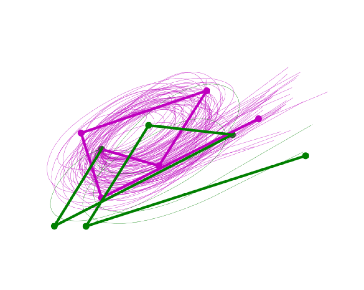
(c) Wedge method.

Figure 14. (2, 6)-clusterings of e characters computed with DBA, CDBA and the wedge method.

Clusters for difficult ‘e’ characters. None of the centers are very clear, but the DBA centers are much more collapsed towards the center and less recognizable than the CDBA and wedge method centers.

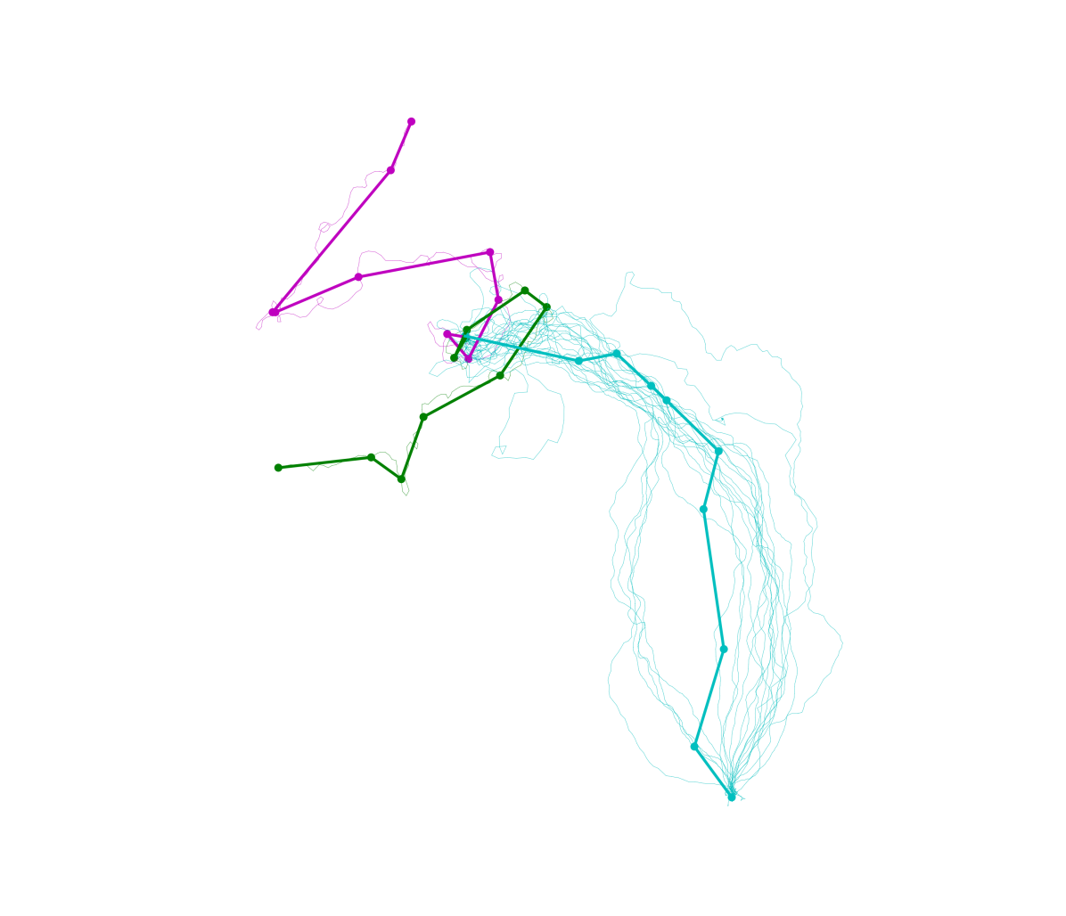
(a) FSA.

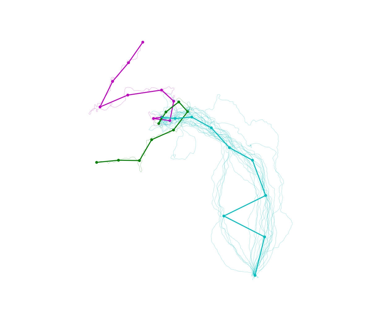
(b) DBA.

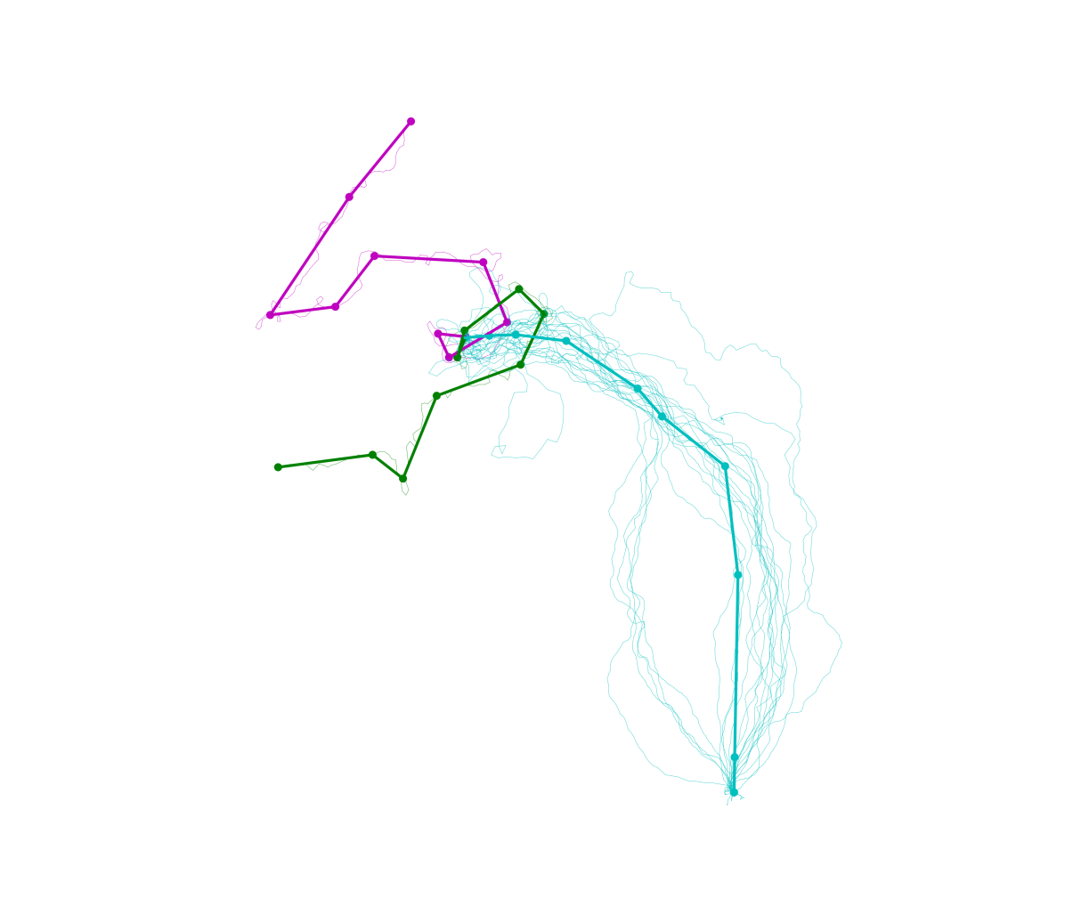
(c) CDBA.

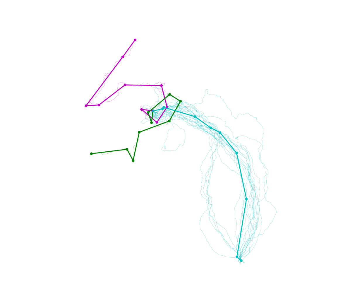
(d) Wedge method.

Figure 15. Centers of an initial clustering updated with (from left to right) FSA, DBA, CDBA, and the wedge method. The trajectory data used is the brc pigeon from the pigeon data set.

The three clusters on pigeon data. FSA has deviations, DBA has a clear jump to one of the trajectories. CDBA and the wedge method produce comparable results that look mostly smoother.

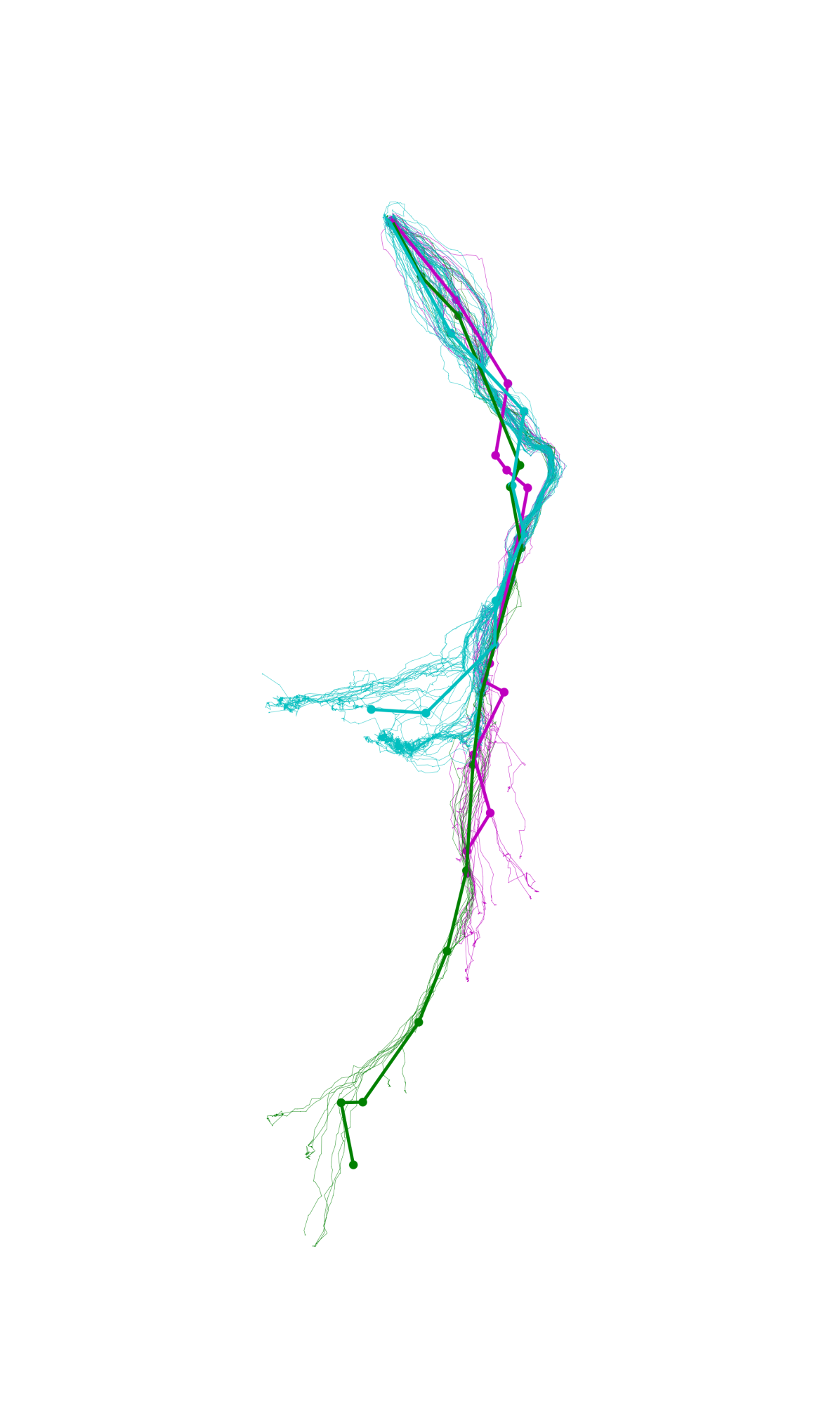
(a) FSA.

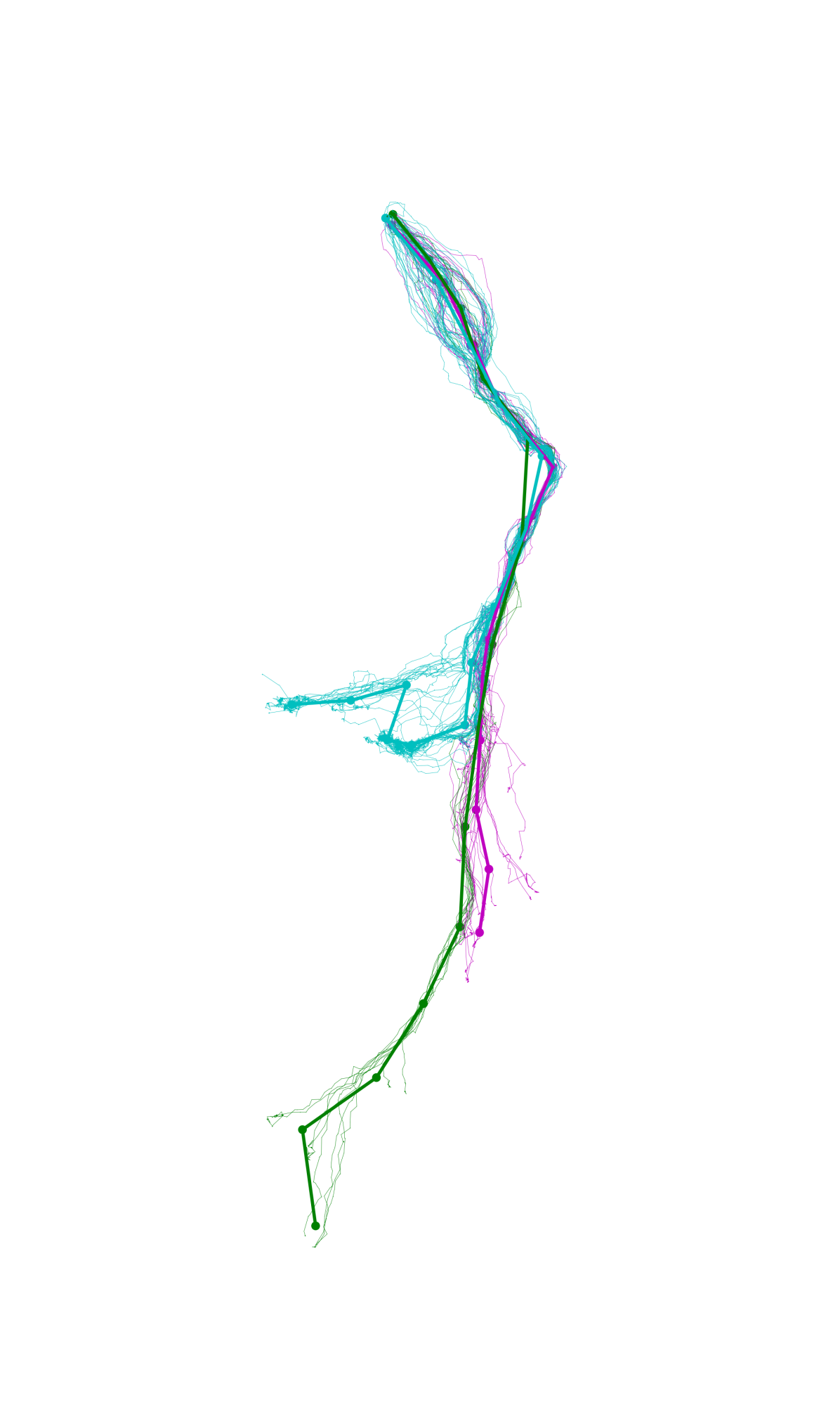
(b) DBA.

(c) CDBA.

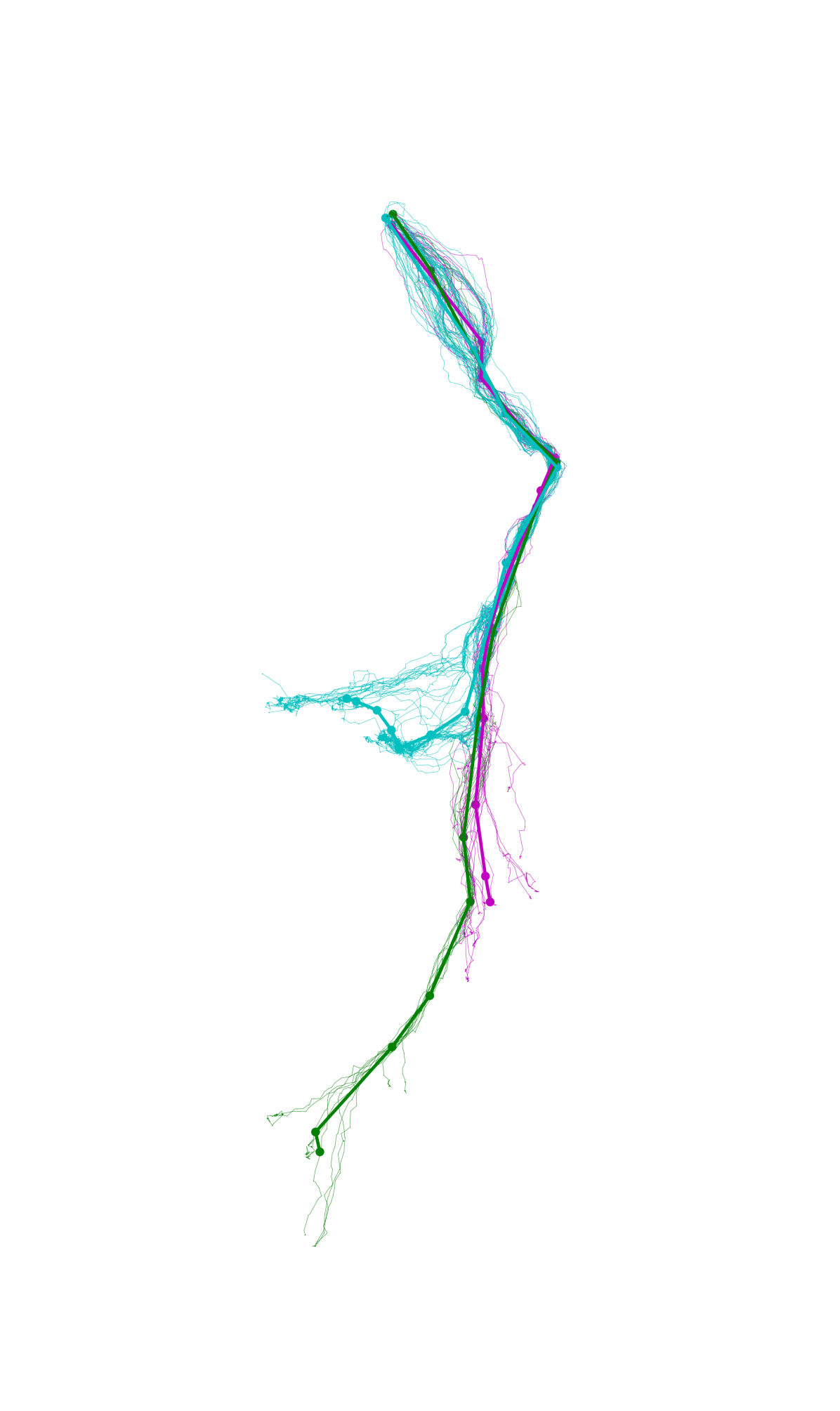
(d) Wedge method.

Figure 16. Centers of an initial clustering updated with (from left to right) FSA, DBA, CDBA, and the wedge method. The trajectory data used is the movebank stork migration data set.

The clusters on the stork migration set. The FSA center has noticeable artifacts and does not follow the trajectories in a visually convincing way. The DBA center ignores a noticeable sideways bend in the trajectories, and so follows the trajectories worse visually than CDBA and the wedge method. CDBA and the wedge method produce visually very similar results.