This paper introduces a general framework to quantify the reliability of the predictions of a dynamical model in the presence of unmeasurable variables, and presents an application to COVID-19.

Lack of practical identifiability may hamper reliable predictions in COVID-19 epidemic models

Compartmental models are widely adopted to describe and predict the spreading of infectious diseases. The unknown parameters of such models need to be estimated from the data. Furthermore, when some of the model variables are not empirically accessible, as in the case of asymptomatic carriers of COVID-19, they have to be obtained as an outcome of the model. Here, we introduce a framework to quantify how the uncertainty in the data impacts the determination of the parameters and the evolution of the unmeasured variables of a given model. We illustrate how the method is able to characterize different regimes of identifiability, even in models with few compartments. Finally, we discuss how the lack of identifiability in a realistic model for COVID-19 may prevent reliable forecasting of the epidemic dynamics.

Introduction

The pandemic caused by SARS-CoV-2 is challenging humanity in an unprecedented way  (?), with the disease that in a few months has spread around the world affecting large parts of the population  (?, ?) and often requiring hospitalization or even intensive care  (?, ?). Mitigating the impact of COVID-19 urges synergistic efforts to understand, predict and control the many, often elusive, facets of the complex phenomenon of the spreading of a new virus, from RNA sequencing to the study of the virus pathogenicity and transmissibility  (?, ?), to the definition of suitable epidemic spreading models  (?) and the investigation of non-pharmaceutical intervention policies and containment measures  (?, ?, ?, ?). In particular, a large number of epidemic models has been recently proposed to describe the evolution of COVID-19 and evaluate the effectiveness of different counteracting measures, including social distancing, testing and contact tracing  (?, ?, ?, ?, ?, ?). However, even the adoption of well-consolidated modeling techniques, such as the use of mechanistic models at the population level based on compartments, poses fundamental problems. First of all, the very same choice of the dynamical variables to use in a compartmental model is crucial, as such variables should adequately capture the spreading mechanisms and need to be tailored to the specific disease. This step is not straightforward, especially when the spreading mechanisms of the disease are still unknown or only partially identified. In addition, some of the variables considered might be difficult to measure and track, as, for instance, it occurs in the case of COVID-19 for the number of individuals showing mild or no symptoms. Secondly, compartmental models, usually, involve a number of parameters, including the initial values of the unmeasured variables, which are not known and need to be estimated from data.

Having at disposal large amount of data, unfortunately, does not simplify the problem of parameter estimation and prediction of unmeasured states. In fact, once a model is formulated, it may occur that some of its unknown parameters are intrinsically impossible to determine from the measured variables, or that they are numerically very sensitive to the measurements themselves. In the first case, it is the very same structure of the model to hamper parameter estimation, as the system admits infinitely many sets of parameters that fit the data equally well; for this reason, this problem is referred to as structural identifiability  (?, ?). In the second case, although, under ideal conditions (i.e., noise-free data and error-free models) the problem of parameter estimation can be uniquely solved, for some trajectories it may be numerically ill-conditioned, such that, from a practical point of view, the parameters cannot be determined with precision even if the model is structurally identifiable. This situation typically occurs when large changes in the parameters entail a small variation of the measured variables, such that two similar trajectories may correspond to very different parameters  (?). The term practical identifiability is adopted in this case.

Identifiability in general represents an important property of a dynamical system, as in a non-identifiable system different sets of parameters can produce the same or very similar fits of the data. Consequently, predictions from a non-identifiable system become unreliable. In the context of epidemics forecasting, this means that even if the model considered is able to reproduce the measured variables, a large uncertainty may affect the estimated values of the parameters and the predicted evolution of the unmeasured variables  (?). Although the problem of structural identifiability has been investigated already for a large number of COVID-19 epidemic models  (?), the more subtle problem of the practical identifiability of such models has not been faced yet. Moreover, in the few existing studies on the practical identifiability of epidemiological models, only the sensitivity of measured variables to the parameters of the model has been considered, and mainly through numerical simulations  (?, ?).

In this paper we investigate the problem of the practical identifiability of dynamical systems whose state includes not only measurable but also hidden variables, as is the case of compartment models for COVID-19 epidemic. We present a novel and general framework to quantify not only the sensitivity of the measured variables of a given model on its parameters, but also the sensitivity of the unmeasured variables on the parameters and on the measured variables. This will allow us to introduce the notion of practical identifiability of the hidden variables of a model. As a relevant and timely application we show the variety of different regimes and levels of identifiability that can appear in epidemic models, even in the simplest case of a four compartment system. Finally, we study the actual effects of the lack of practical identifiability in more sophisticated models recently introduced for COVID-19.

Results

Dynamical systems with hidden variables

Consider the $n$-dimensional dynamical system described by the following equations

$$\begin{array}[]{lll}\dot{\mathbf{m}}&=&\mathbf{f}(\mathbf{m},\mathbf{h},\mathbf{q}),\\ \dot{\mathbf{h}}&=&\mathbf{g}(\mathbf{m},\mathbf{h},\mathbf{q}),\end{array}$$ (1)

where we have partitioned the state variables into two sets, the variables $\mathbf{m}\in\mathbb{R}^{n_{m}}$ that can be empirically accessed (measurable variables), and those, $\mathbf{h}\in\mathbb{R}^{n_{h}}$, with $n_{m}+n_{h}=n$, that cannot be measured (hidden). The dynamics of the system is governed by the two Lipschitz-continuous functions $\mathbf{f}$ and $\mathbf{g}$, which also depend on a vector of structural parameters $\mathbf{q}\in\Omega_{q}\subset\mathbb{R}^{n_{q}}$. The trajectories $\mathbf{m}(t)$ and $\mathbf{h}(t)$ of system (1) are uniquely determined by the structural parameters $\mathbf{q}$ and by the initial conditions $\mathbf{m}(0)=\mathbf{m}_{0},\mathbf{h}(0)=\mathbf{h}_{0}$. Here, we assume that some of the quantities $\mathbf{q}$ are known, while the others are not known and need to be determined by fitting the trajectories of measurable variables $\mathbf{m}(t)$. We denote by $\mathbf{p}\in\Omega_{p}\subset\mathbb{R}^{n_{p}}$ the set of unknown parameters that identify the trajectories, which comprises the unknown terms of $\mathbf{q}$ and the unknown initial conditions $\mathbf{h}_{0}$. The initial values of the hidden variables are not known, and act indeed as parameters for the trajectories generated by system (1). The initial conditions of the measurable variables $\mathbf{m}_{0}$ may be considered fitting parameters as well.

System (1) is said to be structurally identifiable when the measured variables satisfy  (?)

$$\mathbf{m}(t,\hat{\mathbf{p}})=\mathbf{m}(t,\mathbf{p}),\forall t\geq 0\Rightarrow\hat{\mathbf{p}}=\mathbf{p}$$ (2)

for almost any $\mathbf{p}\in\Omega_{p}$. Notice that, as a consequence of the existence and uniqueness theorem for the initial value problem, if system (1) is structurally identifiable, also the hidden variables can be uniquely determined.

Structural identifiability guarantees that two different sets of parameters do not lead to the same time course for the measured variables. Clearly, when this condition is not met, one cannot uniquely associate a data fit to a specific set of parameters or, equivalently, recover the parameters from the measured variables  (?).

Assessing the practical identifiability of a model

Structural identifiability, however, is a necessary but not sufficient condition for parameters estimation, so that, when it comes to use a dynamical system as a model of a real phenomenon, it is fundamental to quantify the practical identifiability of the dynamical system.

To do this, we consider a solution, $\bar{\mathbf{m}}(t)=\mathbf{m}(t,\bar{\mathbf{p}})$ and $\bar{\mathbf{h}}(t)=\mathbf{h}(t,\bar{\mathbf{p}})$, obtained from parameters $\mathbf{p}=\bar{\mathbf{p}}$, and we explore how much the functions $\mathbf{m}(t)$ and $\mathbf{h}(t)$ change as we vary the parameters $\bar{\mathbf{p}}$ by a small amount $\mathbf{\delta p}$. To first order approximation in the perturbation of the parameters, we have $\mathbf{\delta m}=\frac{\partial\mathbf{m}}{\partial\mathbf{p}}\mathbf{\delta p}+\mathcal{O}(\|\mathbf{\delta p}\|^{2})$ and $\mathbf{\delta h}=\frac{\partial\mathbf{h}}{\partial\mathbf{p}}\mathbf{\delta p}+\mathcal{O}(\|\mathbf{\delta p}\|^{2})$. Hence, by dropping the higher order terms we have $\|\mathbf{\delta m}\|^{2}=\int\limits_{0}^{\infty}|\mathbf{\delta m}|^{2}dt=\mathbf{\delta p}^{T}\mathrm{M}\mathbf{\delta p}$ and $\|\mathbf{\delta h}\|^{2}=\int\limits_{0}^{\infty}|\mathbf{\delta h}|^{2}dt=\mathbf{\delta p}^{T}\mathrm{H}\mathbf{\delta p}$, where the entries of the sensitivity matrices $\mathrm{M}=\mathrm{M}(\bar{\mathbf{p}})\in\mathbb{R}^{n_{p}\times n_{p}}$ and $\mathrm{H}=\mathrm{H}(\bar{\mathbf{p}})\in\mathbb{R}^{n_{p}\times n_{p}}$ for the measured and unmeasured variables are defined as

$$\mathrm{(M)}_{ij}=\int\limits_{0}^{\infty}{\frac{\partial\mathbf{m}^{T}}{\partial p_{i}}\frac{\partial\mathbf{m}}{\partial p_{j}}dt};\quad\mathrm{(H)}_{ij}=\int\limits_{0}^{\infty}{\frac{\partial\mathbf{h}^{T}}{\partial p_{i}}\frac{\partial\mathbf{h}}{\partial p_{j}}dt}$$ (3)

Note that these matrices are positive semidefinite by construction. The smallest change in the measured variables $\mathbf{m}(t)$ will take place if $\mathbf{\delta p}$ is aligned along the eigenvector $\mathbf{v}_{1}$ of $\mathrm{M}$ corresponding to the smallest eigenvalue $\lambda_{1}(\mathrm{M})$. Hence, we can consider $\sigma=\sqrt{\lambda_{1}(\mathrm{M})}$ to quantify the sensitivity of the measured variables to the parameters. Practical identifiability requires high values of $\sigma$, as these indicate cases where small changes in the parameters may produce considerable variations of the measurable variables, and therefore the estimation of the model parameters from fitting is more reliable.

Suppose now we consider a perturbation, $\mathbf{\delta p}_{1}$, of the parameters aligned along the direction of $\mathbf{v}_{1}$. We can evaluate the change in $\mathbf{h}(t)$ due to this perturbation by

$$\eta^{2}=\frac{\mathbf{\delta p}_{1}^{T}\mathrm{H}\mathbf{\delta p}_{1}}{\mathbf{\delta p}_{1}^{T}\mathbf{\delta p}_{1}}.$$ (4)

The value of $\eta$ quantifies the sensitivity of the hidden variables to the parameters of the model, when such parameters are estimated from the fitting of the observed variables, since $\|\mathbf{\delta h}\|=\eta\|\mathbf{\delta p}_{1}\|$. Notice that in this case and differently from $\sigma$, lower values of $\eta$ are desirable because imply a better prediction on the hidden variables.

Finally, with the help of the sensitivity matrices defined above, we can also evaluate the sensitivity of the hidden variables to the measured variables as

$$\mu^{2}=\max\limits_{\|\mathbf{\delta p}\|=1}\frac{\mathbf{\delta p}^{T}\mathrm{H}\mathbf{\delta p}}{\mathbf{\delta p}^{T}\mathrm{M}\mathbf{\delta p}}.$$ (5)

This parameter is of particular relevance here, since it provides a bound on how the uncertainty on the measured variables affects the evolution of the hidden variables. In addition, the parameter $\mu^{2}$ can be efficiently computed, as it corresponds to the maximum generalized eigenvalue of matrices $(\mathrm{H}$, $\mathrm{M})$, as shown in Methods.

The sensitivity matrices are useful in studying the effect of changing the number of hidden variables and unknown parameters on the practical identifiability of a model. Assume we have access to one more variable, thus effectively increasing the size of the set of measured variables to $n_{m}^{\prime}=n_{m}+1$ and, correspondingly, reducing that of the unmeasured variables to $n_{h}^{\prime}=n_{h}-1$. This corresponds to consider new variables $\mathbf{m^{\prime}}$ and $\mathbf{h^{\prime}}$. From the definition in Eq. (3), the new sensitivity matrix can be written as $\mathrm{M}^{{}^{\prime}}=\mathrm{M}+\mathrm{M}_{1}$, where $\mathrm{M}_{1}$ is the sensitivity matrix for the newly measured variable. Given Weyl’s inequality ( (?), p. 239) we have that $\lambda_{1}(\mathrm{M}^{\prime})\geq\lambda_{1}(\mathrm{M})+\lambda_{1}(\mathrm{M}_{1})$ and, since $\mathrm{M}_{1}$ is also positive semi-definite, $\lambda_{1}(\mathrm{M}^{\prime})\geq\lambda_{1}(\mathrm{M})$. This means that measuring one further variable (or more than one) of the system increases the practical identifiability of a model, as expected. As $\mathrm{H}^{\prime}=\mathrm{H}-\mathrm{M}_{1}$, it is also possible to demonstrate that $\mu(\mathrm{M}^{\prime})\leq\mu(\mathrm{M})$ (see Materials and Methods). Let us now consider a different scenario: suppose we have a priori knowledge on one of the model parameters, so that we do not need to estimate its value by fitting the model to the data. In this case, we can define new sensitivity matrices $\widetilde{\mathrm{M}},\widetilde{\mathrm{H}}\in\mathbb{R}^{(n_{p}-1)\times(n_{p}-1)}$ for the measured and unmeasured variables respectively. Given the Cauchy’s interlacing theorem ( (?), p. 242), we have that $\lambda_{1}(\widetilde{\mathrm{M}})\geq\lambda_{1}(\mathrm{M})$, which implies that practical identifiability is improved by acquiring a priori information on some of the model parameters. For instance, in the context of COVID-19 models, one may decide to fix some of the parameters, such as the rate of recovery, to values derived from medical and biological knowledge  (?, ?, ?, ?) and to determine from fitting the more elusive parameters, such as the percentage of asymptomatic individuals or the rates of transmission.

The sensitivity measures reveal different regimes of identifiability

As a first application we study the practical identifiability of a four compartment mean-field epidemic model  (?), in the class of SIAR models  (?), developed to assess the impact of asymptomatic carriers of COVID-19  (?, ?, ?) and other diseases  (?, ?, ?). In such a model (Fig. 1), a susceptible individual ($S$) can be infected by an infectious individual who can either be symptomatic ($I$) or asymptomatic ($A$). The newly infected individual can either be symptomatic ($S\rightarrow I$) or asymptomatic ($S\rightarrow A$). Furthermore, we also consider the possibility that asymptomatic individuals develop symptoms ($A\rightarrow I$), thus accounting for the cases in which an individual can infect before and after the onset of the symptoms  (?). Finally, we suppose that individuals cannot be re-infected, as they acquire a permanent immunity ($R$).

Figure 1: Graphical representation of a SIAR model in which infectious individuals can either be symptomatic (I) or asymptomatic (A) (see also Eq. (21) in Materials and Methods).

One of the crucial aspects of COVID-19 is the presence of asymptomatic individuals, which are difficult to trace, as the individuals themselves could be unaware about their state. Consequently, we assume that the fraction of asymptomatic individuals, $a(t)$, is not measurable, while the fractions of symptomatic, $\iota(t)$, and recovered, $r(t)$, are measured variables, that is $\mathbf{m}\equiv[\iota,r]$ and $\mathbf{h}\equiv[s,a]$. As mentioned above, practical identifiability is a property of the trajectories of the system, which are uniquely determined by the values of the unknown parameters $\mathbf{p}$. Here, we illustrate how the sensitivity of both measured and unmeasured variables change with the probability $\gamma$ that a newly infected individual shows no symptoms, when all the other parameters of the model are fixed (to the values reported in Materials and Methods).

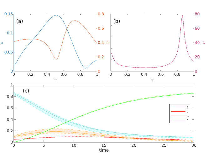
Figure 2: Practical identifiability of the SIAR model in Fig. 1 as a function of the fraction $\gamma$ of asymptomatic new infectious individuals. (a) Sensitivity $\sigma$ and $\eta$ of measured and hidden variables respectively to the parameters of the model. (b) Sensitivity $\mu$ of the hidden variables to the measured ones. (c) State variables for unperturbed values of parameters (with $\gamma=0.86$, solid line) and for a perturbation with $\|\delta\mathbf{p}\|=0.3\|\mathbf{p}\|$ along the first eigenvector of $\mathrm{M}$ (dashed lines).

Fig. 2(a) shows a non-trivial non-monotonic dependence of our sensitivity measures, $\sigma$ and $\eta$, on $\gamma$. The value of $\sigma$ has a peak at $\gamma=0.51$, in correspondence of which $\eta$ takes its minimum value. This represents an optimal condition for practical identifiability, as the sensitivity to parameters of the measured variables is high, while that of the unmeasured ones is low, and this implies that the unknown quantities of the system (both the model parameters and the hidden variables) can be estimated with small uncertainty. On the contrary, for $\gamma=0.86$, we observe a relatively small value of $\sigma$ and a large value of $\eta$, meaning that the measured variables are poorly identifiable, and the unmeasured variables are sensitive to a variation of parameters. This is the worst situation in which the estimated parameters may significantly differ from the real values and the hidden variables may experience large variations even for small changes in the parameters. Furthermore, the quantity $\mu$, which measures the sensitivity of the hidden variables to the measured ones, reported in Fig. 2(b), exhibits a large peak at the value of $\gamma$ for which $\sigma$ is minimal. This is due to the fact that the vector that determines $\mu$ is almost aligned with $\mathbf{v}_{1}$. When this holds, we have that $\mu={\eta}/{\sigma}$, which explains the presence of the spike in the $\mu$ curve. Similarly, the sensitivity $\mu$ takes its minimum almost in correspondence of the maximum of $\sigma$. The behavior of the model for $\gamma=0.86$ is further illustrated in Fig. 2(c), where the trajectories obtained in correspondence to the unperturbed values of the parameters, i.e., $\mathbf{m}(t,\mathbf{p})$ and $\mathbf{h}(t,\mathbf{p})$ (solid lines), are compared with the dynamics observed when $\mathbf{p}$ undergoes a perturbation with $\|\delta\mathbf{p}\|=0.3\|\mathbf{p}\|$ along $\mathbf{v}_{1}$ (dashed lines). The small sensitivity $\sigma$ of the measured variables $\iota(t,\mathbf{p})$ and $r(t,\mathbf{p})$ to parameters, is reflected into perturbed trajectories that remain close to the unperturbed ones, whereas the large sensitivity $\eta$ of the unmeasured variables $s(t,\mathbf{p})$ and $a(t,\mathbf{p})$ yields perturbed trajectories that significantly deviate from the unperturbed ones.

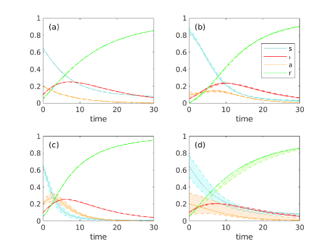
Figure 3: Four scenarios of identifiability for the SIAR model of Fig. 1. All panels show the system dynamics (solid line) and the evolution of the system when the vector of parameters undergoes a variation $\delta\mathbf{p}$ such that $\|\delta\mathbf{p}\|=0.3\|\mathbf{p}\|$ along the first eigenvector of $\mathrm{M}$ (dashed lines). Panels (a) and (c) display configurations for which the observed variables $(\iota,r)$ are not sensitive to the variation, i.e. the model parameters are not identifiable, while panels (b) and (d) show the opposite case. Furthermore, panels (a) and (b) present scenarios for which the unobserved variables $(s,a)$ are insensitive to the variation, meaning that their are predictable, vice-versa panels (c) and (d) show the the case in which the variables $s$ and $a$ are sensitive.

We now illustrate the different levels of identifiability that appears in the SIAR model for diverse settings of the parameters. Its analysis, in fact, fully depicts the more complete perspective on the problem of practical identifiability offered by simultaneously inspecting the sensitivity measures, $\sigma$ and $\eta$. As the two sensitivity measures are not necessarily correlated, there can be cases for which to a high identifiability of the measured variables to the parameters, i.e. large values of $\sigma$, corresponds either a low or a high identifiability of the hidden variables to the parameters. Analogously, for other system configurations, in correspondence of small values of $\sigma$, namely to non-identifiable parameters, one may find large values of $\eta$, meaning that the hidden variables are non-identifiable as well, or, on the contrary small values of $\eta$, indicating that the hidden variables are poorly sensitive to parameter perturbations. Altogether, four distinct scenarios of identifiability can occur and all of them effectively appear in the SIAR model: (a) low identifiability of the model parameters $\mathbf{p}$ and high identifiability of the hidden variables $\mathbf{h}$, (b) high identifiability of both $\mathbf{p}$ and $\mathbf{h}$, (c) low identifiability of both $\mathbf{p}$ and $\mathbf{h}$ and (d) high identifiability of $\mathbf{p}$ and low identifiability of $\mathbf{h}$. To illustrate them, we have considered four distinct configurations of the model (with parameters as given in Table 3, illustrated in Methods) and, for each case study, compared the unperturbed trajectories to the perturbed ones, with the vector of parameters undergoing a variation $\|\delta\mathbf{p}\|=\pm 0.3\|\mathbf{p}\|$, along $\mathbf{v}_{1}$. Fig. 3 shows the results obtained for each parameter configuration. In each panel, the solid lines represent the unperturbed trajectories, while the dashed lines correspond to the perturbed dynamics. In case (a) and (b), we see that, under the variation $\delta\mathbf{p}$, the perturbed trajectories of the hidden variables remain close to the unperturbed dynamics. Hence, the hidden variables are highly identifiable. Conversely, in case (c) and (d), the perturbed trajectories substantially differ from the unperturbed dynamics, meaning that the hidden variables are poorly identifiable, as they are sensitive to a variation of the model parameters. As concerns the measured variables, in cases (a) and (c) the perturbed trajectories slightly differ from the unperturbed dynamics. Therefore, as the measured variables are insensitive to the perturbation $\delta\mathbf{p}$, the model parameters have a low degree of identifiability. On the other hand, in case (b) and (d), the perturbation of the parameters significantly affects the trajectories of the measured variables, meaning that the set of parameters reproducing the observed data is more identifiable.

	(a)	(b)	(c)	(d)
$\sigma$	$0.0096$	$0.15$	$0.013$	$0.091$
$\eta$	$0.012$	$0.16$	$0.36$	$1.4$
$\mu$	$34$	$5.2$	$29$	$15$

Table 1: Values of $\sigma$, $\eta$ and $\mu$ for the four configurations of the SIAR model shown in Fig. 3.

Finally, Table 1 illustrates the values of the sensitivity measures $\sigma$, $\eta$ and $\mu$ for each case. In particular, case (c) represents the worst scenario, as the value of $\sigma$ is relatively small, meaning that the model parameters $\mathbf{p}$ are poorly identifiable, and the value of $\eta$ is large, indicating a high sensitivity of the hidden variables to the parameters. Conversely, the best scenario is represented by case (b), for which both the model parameters and the hidden variables are highly identifiable, as the value of $\sigma$ is large compared to the other cases while the value of $\eta$ remains relatively small.

Lack of identifiability in COVID-19 modeling prevents reliable forecasting

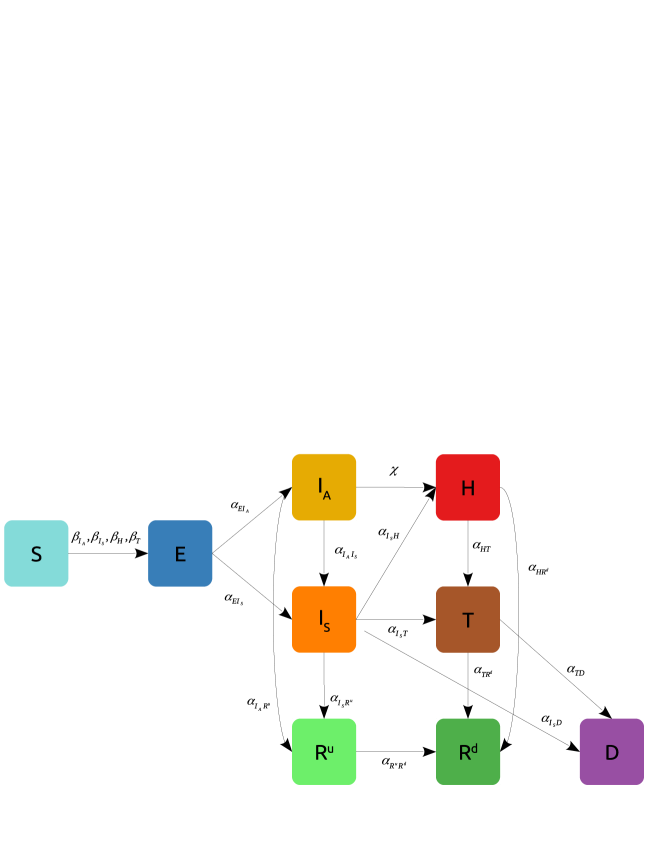
Figure 4: Graphical representation of a nine-compartment model for the propagation of COVID-19 (see also Eq. (22) in Materials and Methods).

As a second application we show the relevance of the problem of practical identifiability in the context of COVID-19 pandemic modeling. We consider a realistic model (Fig. 4) of the disease propagation, that is a variant of the SIDARTHE model  (?) and is characterized by nine compartments accounting respectively for susceptible ($S$), exposed ($E$), undetected asymptomatic ($I_{A}$), undetected symptomatic ($I_{S}$), home isolated ($H$), treated in hospital ($T$), undetected recovered ($R^{u}$), detected recovered ($R^{d}$) and deceased ($D$) individuals. Following  (?), in order to account for the different non-pharmaceutical interventions and testing strategies issued during the COVID-19 outbreak in Italy  (?, ?), the model parameters have been considered piece-wise constant, and estimated, using nonlinear optimization, by fitting of the official data provided by the Civil Protection Department  (?). The available data, namely the daily number of home isolated, hospitalized, detected recovered and deceased individuals, are shown as coloured circles in Fig. 5. Accordingly, we have considered four measured and five hidden variables in the model: $\mathbf{m}\equiv[H,T,R^{d},D]$ and $\mathbf{h}\equiv[S,E,I_{A},I_{S},R^{u}]$.

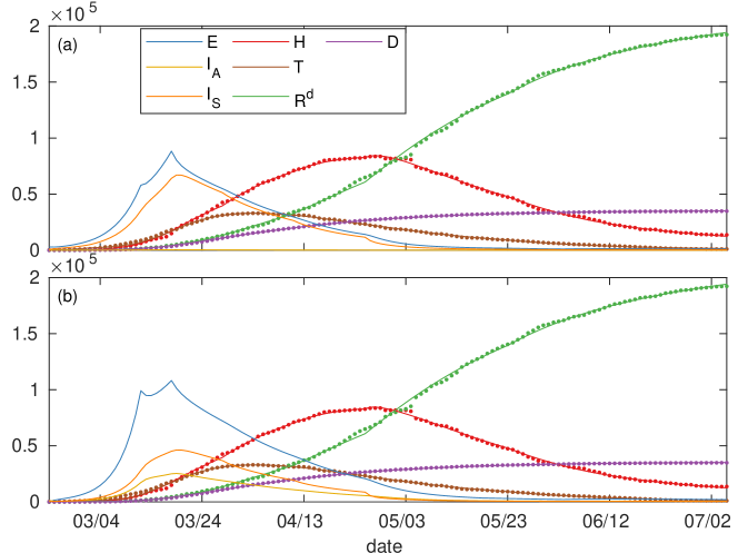
Figure 5: Modelling the COVID-19 outbreak in Italy. The evolution of both hidden and measured variables of the model in Fig. 4 (continuous lines) is reported together with the official data from the Civil Protection Department (circles). (a) and (b) refer to two different sets of parameters $\bf p$ of the model, which fit equally well the available data.

The two panels (a) and (b) of Fig. 5 display the prediction of the model for two sets of the parameters, which have been obtained by allowing different ranges of parameter values for the fitting (see Materials and Methods). Although the model fits equally well the empirical data on the observed variables in the two cases, fundamental differences in the trend of the hidden variables appear. In particular, in case (a) the model predicts a number of asymptomatic individuals, $I_{A}$, which is practically zero throughout the entire outbreak, indicating that all the infectious individuals are symptomatic. Instead, a significant population of asymptomatic individuals (25343 in its peak at day 26) is observed in case (b) and, correspondingly, the size of the symptomatic population is consistently smaller than in case (a).

The two scenarios also lead to remarkable discrepancies in the values of the parameters obtained through fitting. Let us consider, for instance, the rates $\alpha_{EI_{A}}$ and $\alpha_{EI_{S}}$, providing information on the percentage of infected individuals not developing symptoms. In scenario (a) $\alpha_{EI_{A}}=1/18.5$ days^-1 and $\alpha_{EI_{S}}=1/2.5$ days^-1, such that $12\%$ of the newly infected individuals are asymptomatic, while in scenario (b) $\alpha_{EI_{A}}=1/7$ days^-1 and $\alpha_{EI_{S}}=1/6$ days^-1, which signifies that only $45\%$ of the individuals do not develop symptoms after the latency period.

These findings have relevant implications. In fact, the large uncertainty on the size of the asymptomatic population makes questionable the use of the model as a tool to decide the policies to adopt, as it is equally consistent with two scenarios corresponding to two extremely different dynamics of the epidemic.

Discussion

The practical identifiability of a dynamical model is a critical, but often neglected, issue in determining the reliability of its predictions. In this paper we have introduced a novel framework to quantify: 1) the sensitivity of the dynamical variables of a given model to its parameters, even in the presence of variables that are difficult to access empirically; 2) how changes in the measured variables impact the evolution of the unmeasured ones. The set of easily computable measures we have introduced enable to assess, for instance, if and when the model predictions on the unmeasured variables are reliable or not, even when the parameters of the model can be fitted with high accuracy from the available data. As we have shown with a series of case studies, practical identifiability can critically affect the predictions of even very refined epidemic models recently introduced for the description of COVID-19, where dynamical variables, such as the population of asymptomatic individuals, are impossible or difficult to measure. This, by no means, should question the importance of such models, in that they enable a scenario analysis, otherwise impossible to carry out, and a deeper understanding of the spreading mechanisms of a novel disease, but should hallmark the relevance of a critical analysis of the results that takes into account sensitivity measures. It also highlights the importance of cross-disciplinary efforts that can provide a priori information on some of the parameters, ultimately improving the reliability of a model  (?, ?).

Materials and Methods

The sensitivity matrices and their properties

The sensitivity matrices considered in this paper are given by

$$\mathrm{M}_{ij}=\int\limits_{0}^{\infty}{\frac{\partial\mathbf{m}^{T}}{\partial p_{i}}\frac{\partial\mathbf{m}}{\partial p_{j}}dt};\quad\mathrm{H}_{ij}=\int\limits_{0}^{\infty}{\frac{\partial\mathbf{h}^{T}}{\partial p_{i}}\frac{\partial\mathbf{h}}{\partial p_{j}}dt},$$ (6)

where the vector functions $\mathbf{m}=\mathbf{m}(t;\mathbf{p})$ and $\mathbf{h}=\mathbf{h}(t;\mathbf{p})$ are obtained integrating system (1). The derivative of measurable and hidden variables with respect to the parameters $\mathbf{p}$,

$$\mathbf{m}_{i}\equiv\partial{\mathbf{m}}/\partial p_{i},\quad\mathbf{h}_{i}\equiv\partial{\mathbf{h}}/\partial p_{i}$$

can be obtained by integrating the system

$$\begin{array}[]{lll}\displaystyle\frac{d\mathbf{m}_{i}}{dt}&=&\displaystyle\frac{\partial\mathbf{f}}{\partial\mathbf{m}}\cdot\mathbf{m}_{i}+\frac{\partial\mathbf{f}}{\partial\mathbf{h}}\cdot\mathbf{h}_{i}+\frac{\partial\mathbf{f}}{\partial p_{i}},\\[14.22636pt] \displaystyle\frac{d\mathbf{h}_{i}}{dt}&=&\displaystyle\frac{\partial\mathbf{g}}{\partial\mathbf{m}}\cdot\mathbf{m}_{i}+\frac{\partial\mathbf{g}}{\partial\mathbf{h}}\cdot\mathbf{h}_{i}+\frac{\partial\mathbf{g}}{\partial p_{i}},\end{array}$$ (7)

where $i=1,\dots n_{p}$.

The numerical evaluation of the sensitivity matrices is carried out, first integrating system (7) (for this step we use a fourth-order Runge-Kutta solver with adaptive step size control), resampling the trajectories with a sampling period of 1 day, and, then, performing a discrete summation over the sampled trajectories. Moreover, integration is carried out over a finite time interval $[0,\tau]$, with large enough $\tau$. In the context of our work, as we have considered SIR-like epidemic models, we set the value of $\tau$ such that the system has reached a stationary state, i.e. the epidemic outbreak has ended, as every infected individual has eventually recovered (or dead, depending on the model).

We now present an important property of the sensitivity matrices. We will only take into account the set of measured variables $\mathbf{m}$, as similar considerations can be made for the hidden variables. Let us assume to be able to measure only a single variable, so that the vector $\mathbf{m}$ collapses into a scalar function, that we call $m_{1}(t)$. In this case, the element $\mathrm{M}_{ij}$ of the sensitivity matrix would be simply given by

$$\mathrm{(M)}_{ij}=\int\limits_{0}^{\infty}{\frac{\partial m_{1}}{\partial p_{i}}\frac{\partial m_{1}}{\partial p_{j}}dt}.$$ (8)

Let us call this sensitivity matrix $\mathrm{M}_{1}$.

Consider now a larger set of measured variables $\mathbf{m}=(m_{1},m_{2},\dots,m_{n_{m}})$. The quantity $\partial\mathbf{m}^{T}/\partial p_{i}\partial\mathbf{m}/\partial p_{j}$ in Eq. (6) is given by

$$\frac{\partial\mathbf{m}^{T}}{\partial p_{i}}\frac{\partial\mathbf{m}}{\partial p_{j}}=\frac{\partial m_{1}}{\partial p_{i}}\frac{\partial m_{1}}{\partial p_{j}}+\frac{\partial m_{2}}{\partial p_{i}}\frac{\partial m_{2}}{\partial p_{j}}+\dots+\frac{\partial m_{n_{m}}}{\partial p_{i}}\frac{\partial m_{n_{m}}}{\partial p_{j}}.$$ (9)

Therefore, integrating over time in the interval $[0,\infty)$ and given the linearity property of the integrals, we find that the sensitivity matrix $\mathrm{M}$ of the set of the measured variables is given by the sum of the sensitivity matrices of the single measured variables. Formally we have that

$$\mathrm{M}=\mathrm{M}_{1}+\mathrm{M}_{2}+\dots+\mathrm{M}_{n_{m}}.$$ (10)

This property of the sensitivity matrices is useful to demonstrate how measuring a further variable affects the sensitivity measures $\sigma$ and $\mu$ as discussed in the following subsection and in the Results.

Finally, because matrices $\mathrm{M}$ and $\mathrm{H}$ are positive semidefinite, their eigenvalues are non-negative. For any positive semidefinite matrix $\mathrm{A}$ of order $m$, we shall denote its eigenvalues as $0\leq\lambda_{1}(\mathrm{A})\leq\lambda_{2}(\mathrm{A})\leq\dots\leq\lambda_{m}(\mathrm{A})$.

Sensitivity measures and their properties

Here, we discuss in more detail the sensitivity measures introduced in the Results. First, we want to propose a measure to quantify the practical identifiability of the model parameters given the measured variables. To do this, we need to evaluate the sensitivity of the trajectories of the measured variables to a variation of the model parameters. In fact, if this sensitivity is small, then different sets of parameters will produce very similar trajectories of the measured variables, meaning that the parameters themselves are poorly identifiable. In particular, as a measure of the parameters identifiability, we can consider the worst scenario, namely the case in which the perturbation of the parameters minimizes the change in the measured variables. This happens when the variation of the model parameters $\mathbf{\delta p}$ is aligned along the eigenvector $\mathbf{v}_{1}$ of $\mathrm{M}$ corresponding to the minimum eigenvalue $\lambda_{1}(\mathrm{M})$. Given the definition of $\mathrm{M}$ we have that $\|\delta\mathbf{m}\|=\sqrt{\lambda_{1}(\mathrm{M})}\,\|\delta\mathbf{p}\|$, hence we can consider the quantity

$$\sigma=\sqrt{\lambda_{1}(\mathrm{M})}$$ (11)

as an estimate of the sensitivity of the measured variables to the parameters. Note that, here and in the rest of the paper, $\|\mathbf{v}\|$ denotes the Euclidean norm of a finite dimensional vector $\mathbf{v}$, $\|\mathbf{v}\|^{2}=\mathbf{v}\cdot\mathbf{v}$, while for a function $\mathbf{u}(t)$, $\|\mathbf{u}\|$ denotes the $L^{2}$ norm of $\mathbf{u}$ in $[0,\infty]$, i.e. $\|\mathbf{u}\|^{2}=\int_{0}^{\infty}\mathbf{u}\cdot\mathbf{u}\,dt$.

Let us now focus on the hidden variables $\mathbf{h}$. In general, as the hidden variables are not directly associated to empirical data, the largest uncertainty on the hidden variables is obtained in correspondence of a variation of the parameters along the eigenvector of $\mathrm{H}$ associated to the largest eigenvalue, namely $\lambda_{n_{p}}(\mathrm{H})$. Hence, to quantify the sensitivity of the hidden variables to the parameters, one may consider

$$\eta_{MAX}=\sqrt{\lambda_{n_{p}}(\mathrm{H})}.$$ (12)

However, it is crucial to note that the hidden variables ultimately depend on the parameters of the model, which are estimated by fitting data that are available for the measured variables only. As a consequence, it is reasonable to consider a quantity that evaluates how the uncertainty on the model parameters (determined by the uncertainty of the measured variables and by their sensitivity to the parameters) affects the identifiability of the hidden variables. Therefore, as a measure of the sensitivity of the hidden variables to the parameters we consider

$$\eta^{2}=\frac{\delta\mathbf{p}_{1}^{T}\mathrm{H}\delta\mathbf{p}_{1}}{\delta\mathbf{p}_{1}^{T}\delta\mathbf{p}_{1}},$$ (13)

where $\delta\mathbf{p}_{1}$ is a perturbation of the parameters along the eigenvector $\mathbf{v}_{1}$ of $\mathrm{M}$ corresponding to the minimum eigenvalue $\lambda_{1}(\mathrm{M})$. Note that, when $\mathbf{v}_{1}$ and the eigenvector of $\mathrm{H}$ corresponding to the largest eigenvalue $\lambda_{n_{p}}(\mathrm{H})$ are aligned, by definition we have $\eta=\eta_{MAX}$.

Finally, we want to define a quantity to estimate how much the hidden variables are perturbed given a variation of the measured ones. In particular, as a measure of the sensitivity of the hidden variables to the measured variables, we consider the maximum perturbation of the hidden variables given the minimum variation of the measured ones, which is

$$\mu^{2}=\max\limits_{\|\mathbf{\delta p}\|=1}\frac{\mathbf{\delta p}^{T}\mathrm{H}\mathbf{\delta p}}{\mathbf{\delta p}^{T}\mathrm{M}\mathbf{\delta p}}.$$ (14)

Note that $\mu^{2}$ can be computed considering the following generalized eigenvalue problem

$$\mathrm{H}\mathbf{u}_{k}=\lambda_{k}\mathrm{M}\mathbf{u}_{k},$$ (15)

where $\mathrm{H}$ and $\mathrm{M}$ are the sensitivity matrices for the hidden and the observed variables respectively, and $\lambda_{k}=\lambda_{k}(\mathrm{M},\mathrm{H})$ denotes the $k$-th generalized eigenvalue of matrices $\mathrm{M}$ and $\mathrm{H}$. We will denote by $\lambda_{n_{p}}$ the largest generalized eigenvalue, and $\mathbf{u}$ the corresponding generalized eigenvector. Note that, since both matrices are symmetric, if $\mathbf{u}$ is a right eigenvector then $\mathbf{u}^{T}$ is a left eigenvector. Multiplying each member of the equation by $\mathbf{u}^{T}$ and dividing by $\mathbf{u}^{T}\mathrm{M}\mathbf{u}$, we obtain

$$\lambda_{n_{p}}=\frac{\mathbf{u}^{T}\mathrm{H}\mathbf{u}}{\mathbf{u}^{T}\mathrm{M}\mathbf{u}}=\max\limits_{\|\mathbf{v}\|=1}\frac{\mathbf{v}^{T}\mathrm{H}\mathbf{v}}{\mathbf{v}^{T}\mathrm{M}\mathbf{v}},$$ (16)

where one can recognize the definition of $\mu^{2}$ provided in Eq. (14). In other words, $\mu^{2}$ represents the largest eigenvalue of the matrix $\mathrm{M}^{-1}\mathrm{H}$.

It is worth noting two aspects about the sensitivity measure $\mu$. First, given definitions (11) and (12), for any $\delta\mathbf{p}$ with $\|\delta\mathbf{p}\|=1$, we have that $\delta\mathbf{p}^{T}\mathrm{H}\delta\mathbf{p}\leq\eta_{MAX}^{2}$ and $\delta\mathbf{p}^{T}\mathrm{M}\delta\mathbf{p}\geq\sigma^{2}$. As a consequence, we have that

$$\mu^{2}\leq\frac{\eta_{MAX}^{2}}{\sigma^{2}}.$$ (17)

Second, when the vector $\delta\mathbf{p}$ that determines $\mu$ is aligned with the eigenvector $\mathbf{v}_{1}$ of $\mathrm{M}$, it is possible to express $\mu$ in terms of the sensitivity measures $\sigma$ and $\eta$. Indeed, when $\delta\mathbf{p}=\|\delta\mathbf{p}\|\mathbf{v}_{1}=\mathbf{v}_{1}$, recalling definitions (11) and (13), one obtains $\mathbf{v}_{1}^{T}\mathrm{M}\mathbf{v}_{1}=\sigma^{2}$, while $\mathbf{v}_{1}^{T}\mathrm{H}\mathbf{v}_{1}=\eta^{2}$, from which it follows

$$\mu=\frac{\eta}{\sigma}.$$ (18)

Also, we note that if $\mathbf{v}_{1}$ and the eigenvector of $\mathrm{H}$ corresponding to its largest eigenvalue are aligned, one obtains that $\mu=\eta_{MAX}/\sigma$, which is the maximum value for the sensitivity measure $\mu$.

We now demonstrate that the sensitivity of the hidden variables to the measured ones, $\mu^{2}$, decreases as we measure one further variable. Let us assume now we are able to measure one further variable, thus increasing the size of the set of measured variables to $n_{m}^{\prime}=n_{m}+1$ and, correspondingly, reducing that of the unmeasured variables to $n_{h}^{\prime}=n_{h}-1$. Given the property in Eq. (10), the new sensitivity matrices can be written as $\mathrm{M}^{\prime}=\mathrm{M}+\mathrm{M}_{1}$ and $\mathrm{H}^{\prime}=\mathrm{H}-\mathrm{M}_{1}$, where by $\mathrm{M}_{1}$ we denote the sensitivity matrix for the newly measured variable. The new generalized eigenvalue problem is

$$\mathrm{H}^{\prime}\mathbf{u}^{\prime}=\lambda^{\prime}\mathrm{M}^{\prime}\mathbf{u}^{\prime}\Leftrightarrow(\mathrm{H}-\mathrm{M}_{1})\mathbf{u}^{\prime}=\lambda^{\prime}(\mathrm{M}+\mathrm{M}_{1})\mathbf{u}^{\prime},$$ (19)

where, for simplicity, we have denoted by $\lambda^{\prime}$ the largest generalized eigenvalue of matrices $\mathrm{M}^{\prime}$ and $\mathrm{H}^{\prime}$

Left multiplying by $\mathbf{u}^{\prime T}$ and dividing by $\mathbf{u}^{\prime T}\mathrm{M}\mathbf{u}^{\prime}$, we obtain

$$\lambda_{n_{p}}=\frac{\mathbf{u}^{T}\mathrm{H}\mathbf{u}}{\mathbf{u}^{T}\mathrm{M}\mathbf{u}}\geq\frac{\mathbf{u}^{\prime T}\mathrm{H}\mathbf{u}^{\prime}}{\mathbf{u}^{\prime T}\mathrm{M}\mathbf{u}^{\prime}}=\frac{\mathbf{u}^{\prime T}\mathrm{H}^{\prime}\mathbf{u}^{\prime}+\mathbf{u}^{\prime T}\mathrm{M}_{1}\mathbf{u}^{\prime}}{\mathbf{u}^{\prime T}\mathrm{M}\mathbf{u}^{\prime}-\mathbf{u}^{\prime T}\mathrm{M}_{1}\mathbf{u}^{\prime}}\geq\frac{\mathbf{u}^{\prime T}\mathrm{H}^{\prime}\mathbf{u}^{\prime}}{\mathbf{u}^{\prime T}\mathrm{M}^{\prime}\mathbf{u}^{\prime}}=\lambda^{\prime},$$ (20)

where the first inequality comes from the definition of $\lambda_{n_{p}}$, while the second comes from the fact that $\mathrm{H}$, $\mathrm{M}$, $\mathrm{H}^{\prime}$, $\mathrm{M}^{\prime}$ and $\mathrm{M}_{1}$ are positive semidefinite. In short, we find that $\lambda_{n_{p}}\geq\lambda^{\prime}$, meaning that, by measuring one variable, the sensitivity of the hidden variables to the measured ones decreases.

SIAR model and setup for numerical analysis

The SIAR model of Fig. 1 is described by the following equations

$$\begin{cases}\dot{s}=-s(\beta_{I}\iota+\beta_{A}a)\\ \dot{\iota}=(1-\gamma)a(\beta_{I}\iota+\beta_{A}a)+\alpha_{AI}a-\alpha_{IR}\iota\\ \dot{a}=\gamma a(\beta_{I}\iota+\beta_{A}a)-(\alpha_{AI}+\alpha_{AR})a\\ \dot{r}=\alpha_{IR}\iota+\alpha_{AR}a,\end{cases}$$ (21)

where $s(t)$, $\iota(t)$, $a(t)$, and $r(t)$ represent population densities, i.e., $s(t)=S(t)/N$, $\iota(t)=I(t)/N$, $a(t)=A(t)/N$, and $r(t)=R(t)/N$, where $S(t)$, $I(t)$, $A(t)$, and $R(t)$ represent the number of susceptible, infectious, asymptomatic and recovered individuals and $N$ is the size of the population, so that $s(t)+\iota(t)+a(t)+r(t)=1$. Here, $\beta_{I}$ and $\beta_{A}$ are the transmission rates for the symptomatic and the asymptomatic individuals respectively, $\gamma$ is the probability for newly infected individuals to show no symptoms, $\alpha_{AI}$ is the rate at which asymptomatic individuals become symptomatic, and $\alpha_{IR}$ and $\alpha_{AR}$ are the recovery rates for the two infectious populations.

Asymptomatic individuals are difficult to trace, as the individuals themselves could be unaware about their state. As a consequence, we assume that the density of asymptomatic individuals is not measurable, while the densities of symptomatic and recovered individuals are measured variables. According to the notation introduced in Eq. (1), we therefore have that $\mathbf{m}\equiv[\iota,r]$ and $\mathbf{h}\equiv[s,a]$. Note that, as a first approximation, here we assume to be able to trace the asymptomatic individuals once they recover.

The results presented in Fig. 2 have been obtained considering the following setup. As the number of symptomatic infectious and recovered individuals are considered measurable, we have assumed that the initial conditions $\iota(0)$, $r(0)$ and the rate of recovery $\alpha_{I,R}$ are known parameters. Second, we have supposed to be able to measure, for instance through backward contact tracing, the rate at which asymptomatic individuals develop symptoms, i.e., $\alpha_{AI}$. Hence, the vector of parameters to determine by calibrating the model is given by $\mathbf{p}=[a(0),\beta_{I},\beta_{A},\gamma,\alpha_{AR}]$. Table 2 displays the value of the model parameters used to obtain the results shown in Fig. 2.

$\iota_{0}$	$a_{0}$	$r_{0}$	$\beta_{I}$	$\beta_{A}$	$\alpha_{IR}$	$\alpha_{AR}$	$\alpha_{AI}$
$0.05$	$0.1$	$0$	$0.6$	$0.3$	$0.1$	$0.2$	$0.03$

Table 2: Values of the model parameters used for the case study in Fig. 2.

For the analysis of the four scenarios considered in Fig. 3, the values of the model parameters have been set as given in Table 3. Furthermore, to better contrast the results arising in the different case studies, in (a) and (c) we have considered $\mathbf{p}=[\iota(0),a(0),r(0),\beta_{I},\beta_{A},\gamma,\alpha_{IR},\alpha_{AR},\alpha_{AI}]$, while in (b) and (d) we have set $\mathbf{p}=[a(0),\beta_{I},\beta_{A},\gamma,\alpha_{AR}]$.

	$\iota_{0}$	$a_{0}$	$r_{0}$	$\beta_{I}$	$\beta_{A}$	$\gamma$	$\alpha_{IR}$	$\alpha_{AR}$	$\alpha_{AI}$
(a)	$0.1$	$0.2$	$0.05$	$0.3$	$0.4$	$0.26$	$0.1$	$0.2$	$0.03$
(b)	$0.05$	$0.1$	$0$	$0.6$	$0.3$	$0.51$	$0.1$	$0.2$	$0.03$
(c)	$0.1$	$0.2$	$0.05$	$0.6$	$0.8$	$0.77$	$0.1$	$0.2$	$0.1$
(d)	$0.1$	$0.2$	$0.05$	$0.3$	$0.4$	$0.53$	$0.1$	$0.2$	$0.03$

Table 3: Values of the model parameters used for the case study in Fig. 3

Nine compartment model for COVID-19

The nine compartment model of Fig. 4 can be considered as a variant of the SIDARTHE model  (?). It is characterized by the presence of an incubation state, in which the individuals have been exposed to the virus ($E$) but are not yet infectious, and by infectious individuals, that, in addition to being symptomatic or asymptomatic, can be either detected or undetected. The model, therefore, includes four classes of infectious individuals: undetected asymptomatic ($I_{A}$), undetected symptomatic and pauci-symptomatic ($I_{S}$), home isolated ($H$, corresponding to detected asymptomatic and pauci-symptomatic), and treated in hospital ($T$, corresponding to detected symptomatic). Finally, removed individuals can be undetected ($R^{u}$), detected ($R^{d}$) or deceased ($D$).

The model dynamics is described by the following equations

$$\left\{\begin{array}[]{lll}\dot{S}&=&-S(\beta_{I_{A}}I_{A}+\beta_{I_{S}}I_{S}+\beta_{H}H+\beta_{T}T)/N\\ \dot{E}&=&\>\phantom{-}\>S(\beta_{I_{A}}I_{A}+\beta_{I_{S}}I_{S}+\beta_{H}H+\beta_{T}T)/N\\ &&-(\alpha_{EI_{A}}+\alpha_{EI_{S}})E\\ \dot{I}_{A}&=&\>\displaystyle\alpha_{EI_{A}}E-(\alpha_{I_{A}I_{S}}+\alpha_{I_{A}R^{u}})I_{A}-\chi I_{A}\\ \dot{I_{S}}&=&\>\alpha_{EI_{S}}E+\alpha_{I_{A}I_{S}}I_{A}\\ &&-(\alpha_{I_{S}H}+\alpha_{I_{S}T}+\alpha_{I_{S}R^{u}}+\alpha_{I_{S}D})I_{S}\\ \dot{H}&=&\>\alpha_{I_{S}H}I_{S}+\chi I_{A}-(\alpha_{HT}+\alpha_{HR^{d}})H\\ \dot{T}&=&\>\alpha_{I_{S}T}I_{S}+\alpha_{HT}H-(\alpha_{T,R^{d}}+\alpha_{TD})T\\ \dot{R}^{u}&=&\>\alpha_{I_{A}R^{u}}I_{A}+\alpha_{I_{S}R^{u}}I_{S}\\ \dot{R}^{d}&=&\>\alpha_{HR^{d}}H+\alpha_{TR^{d}}T\\ \dot{D}&=&\>\alpha_{I_{S}D}I_{S}+\alpha_{TD}T,\end{array}\right.$$ (22)

where the state variables represent the number of individuals in each compartment, $N=60\cdot 10^{6}$ and $S+E+I_{A}+I_{S}+H+T+R^{u}+R^{d}+D=N$. The official data on the spreading of COVID-19 in Italy made available by the Civil Protection Department (Dipartimento della Protezione Civile,  (?)) provide information only on four of the nine compartments of the model, namely the home isolated ($H$), hospitalized ($T$), detected recovered ($R^{d}$) and deceased individuals ($D$). These compartments constitute the set of the measured variables, while the other variables have to be considered as hidden, that is $\mathbf{m}\equiv[H,T,R^{d},D]$ and $\mathbf{h}\equiv[S,E,I_{A},I_{S},R^{u}]$.

All the parameters appearing in (22) are considered unknown, thus they need to be determined through fitting the model to the available data. It should also be noted that, as many non-pharmaceutical interventions have been issued/lifted and the testing strategy has been changed several times over the course of the epidemics  (?, ?), not all parameters can be considered constant in the whole period used for the fitting. Hence, similarly to  (?), we have divided the whole period of investigation (which in our case ranges from February 24 to July 6, 2020) into different windows, within each of which the parameters are assumed to be constant. In each time window, one allows only some parameters to vary, according to what is reasonable to assume will be influenced by the government intervention during that time window.

We distinguish two kinds of events that may require an adaptation of the model parameters. On the one hand, there are the non-pharmaceutical containment policies, aimed at reducing the disease transmission. When such interventions are issued, the value of the parameters $\beta$ may vary. On the other hand, the testing strategy, which affects the probability of detecting infected individuals, was also not uniform in the investigated period. When the testing policy changes, the value of the parameters $\alpha_{I_{S}H}$, $\alpha_{HT}$ and $\alpha_{HR^{d}}$ may vary. Here, we notice two important points. First, the value of $\alpha_{I_{S}T}$ is assumed to be constant in the whole period, as we suppose that there are no changes in how the symptomatic individuals requiring hospitalization are detected. Second, as a change in the sole parameter $\alpha_{I_{S}H}$ would affect too much the average time an individual remains infected, then also $\alpha_{HT}$ and $\alpha_{HR^{d}}$ have to be included in the set of parameters that may change. Based on these considerations, the intervals in which each parameter remains constant or may change are identified. This defines the specific piece-wise waveform assumed for each of the parameters appearing in the model and, consequently, the effective number of values that need to be estimated for each parameter.

Hereafter, we summarize the events defining the different windows in which the whole period of investigation is partitioned:

1. On March 2, a policy limiting screening only to symptomatic individuals is introduced.

2. On March 12, a partial lockdown is issued.

3. On March 18, a stricter lockdown, which further limits non-essential activities, is imposed.

4. On March 28, a wider testing campaign is launched. Starting from this date, as the number of tests has constantly increased, while the number of new infections was decreasing, the parameters are allowed to change every 14 or 28 days, namely on April 11, April 25 and May 23.

5. On May 4, a partial lockdown lift is proclaimed.

6. On May 18, further restrictions are relaxed.

7. On June 3, inter-regional mobility is allowed. This is the last time the model parameters are changed.

Note that, for the time period until April 5, we have followed the same time partition used in  (?).

The model parameters have been estimated using a nonlinear optimization procedure (implemented via the function mincon } in MATLAB) with the ollowing objective function to minimize

$$e=\sqrt{\frac{1}{4\tau}\sum\limits_{k=1}^{\tau}\left((H(k)-\bar{H}(k))^{2}+(T(k)-\bar{T}(k))^{2}+(R^{d}(k)-\bar{R}^{d}(k))^{2}+(D(k)-\bar{D}(k))^{2}\right)}$$ (23)

where $\bar{H}(k)$, $\bar{T}(k)$, $\bar{R}^{d}(k)$, and $\bar{D}(k)$ with $k=1,\ldots,\tau$ ($\tau=134$ days) represent the time series of daily data for isolated, hospitalized, detected recovered and deceased individuals provided by the Civil Protection Department  (?), and ${H}(k)$, ${T}(k)$, $\bar{R}^{d}(k)$, and $\bar{D}(k)$ are the values of the corresponding variables obtained from the integration of Eqs. (22). The integration of Eqs. (22) has been carried out by using a suitable ODE solver with maximum integration step size equal to $10^{-2}$ days and then resampling the data with a sampling period of 1 day.

Fig. 3 displays two distinct fits of model (22). Here, we provide further details on how they have been obtained. In case b), upper and lower bounds on the parameters $\alpha_{EI_{A}}$ and $\alpha_{EI_{S}}$ have been incorporated in the parameter estimation procedure, thus constraining the percentage of asymptomatic individuals $p_{A}=\alpha_{EI_{A}}/(\alpha_{EI_{A}}+\alpha_{EI_{S}})$, while in case (a) no constraint has been considered. In more detail, in case (b), we fixed $30\%\leq p_{A}\leq 50\%$  (?) and also imposed $\alpha_{EI_{S}}/2\leq\alpha_{EI_{A}}\leq\alpha_{EI_{S}}$. In both cases the model fits well the empirical data on the observed variables [the fitting error (23) is $e=898$ individuals in case (a) and $e=938$ individuals in case (b)], but fundamental differences in the trend of the hidden variables appear. In particular, in scenario (a), which does not include constraints on the percentage of asymptomatic individuals, the compartment $I_{A}$ is approximately zero throughout the entire epidemics, indicating that all the undetected infectious individuals are symptomatic. Vice-versa, in scenario (b) a number of undetected asymptomatic individuals appears, and, correspondingly, the population of undetected symptomatic individuals is consistently smaller than in case (a).

Author contributions

L.G., M.F., V.L. and G.R. conceived the research and developed the theory. L.G. carried out the numerical analysis. All authors wrote the manuscript.

Competing interests

The authors declare they have no competing interests.

Data and material availability

All data needed to evaluate the results are present in the paper itself. Additional data related to this paper may be requested to the authors.

References

- 1. R. M. Anderson, H. Heesterbeek, D. Klinkenberg, T. D. Hollingsworth, How will country-based mitigation measures influence the course of the covid-19 epidemic? The Lancet 395, 931–934 (2020).
- 2. World Health Organization (WHO), Coronavirus disease (covid-19): weekly epidemiological update, https://www.who.int/emergencies/diseases/novel-coronavirus-2019/situation-reports (2020). Accessed: 2020-10-15.
- 3. E. Dong, H. Du, L. Gardner, An interactive web-based dashboard to track covid-19 in real time. The Lancet infectious diseases 20, 533–534 (2020).
- 4. C. Huang, Y. Wang, X. Li, L. Ren, J. Zhao, Y. Hu, L. Zhang, G. Fan, J. Xu, X. Gu, et al., Clinical features of patients infected with 2019 novel coronavirus in wuhan, china. The lancet 395, 497–506 (2020).
- 5. N. Chen, M. Zhou, X. Dong, J. Qu, F. Gong, Y. Han, Y. Qiu, J. Wang, Y. Liu, Y. Wei, et al., Epidemiological and clinical characteristics of 99 cases of 2019 novel coronavirus pneumonia in wuhan, china: a descriptive study. The Lancet 395, 507–513 (2020).
- 6. W. J. Wiersinga, A. Rhodes, A. C. Cheng, S. J. Peacock, H. C. Prescott, Pathophysiology, transmission, diagnosis, and treatment of coronavirus disease 2019 (covid-19): a review. Jama 324, 782–793 (2020).
- 7. L.-s. Wang, Y.-r. Wang, D.-w. Ye, Q.-q. Liu, A review of the 2019 novel coronavirus (covid-19) based on current evidence. International journal of antimicrobial agents p. 105948 (2020).
- 8. E. Estrada, Covid-19 and sars-cov-2. modeling the present, looking at the future. Physics Reports (2020).
- 9. M. Chinazzi, J. T. Davis, M. Ajelli, C. Gioannini, M. Litvinova, S. Merler, A. P. y Piontti, K. Mu, L. Rossi, K. Sun, et al., The effect of travel restrictions on the spread of the 2019 novel coronavirus (covid-19) outbreak. Science 368, 395–400 (2020).
- 10. K. Leung, J. T. Wu, D. Liu, G. M. Leung, First-wave covid-19 transmissibility and severity in china outside hubei after control measures, and second-wave scenario planning: a modelling impact assessment. The Lancet (2020).
- 11. P. Castorina, A. Iorio, D. Lanteri, Data analysis on coronavirus spreading by macroscopic growth laws. International Journal of Modern Physics C p. 2050103 (2020).
- 12. D. Lanteri, D. Carcò, P. Castorina, M. Ceccarelli, B. Cacopardo, Containment effort reduction and regrowth patterns of the covid-19 spreading. arXiv preprint arXiv:2004.14701 (2020).
- 13. D. Fanelli, F. Piazza, Analysis and forecast of covid-19 spreading in china, italy and france. Chaos, Solitons & Fractals 134, 109761 (2020).
- 14. A. Arenas, W. Cota, J. Gomez-Gardenes, S. Gómez, C. Granell, J. T. Matamalas, D. Soriano-Panos, B. Steinegger, A mathematical model for the spatiotemporal epidemic spreading of covid19. MedRxiv (2020).
- 15. A. J. Kucharski, T. W. Russell, C. Diamond, Y. Liu, J. Edmunds, S. Funk, R. M. Eggo, F. Sun, M. Jit, J. D. Munday, et al., Early dynamics of transmission and control of covid-19: a mathematical modelling study. The lancet infectious diseases (2020).
- 16. G. Giordano, F. Blanchini, R. Bruno, P. Colaneri, A. Di Filippo, A. Di Matteo, M. Colaneri, Modelling the covid-19 epidemic and implementation of population-wide interventions in italy. Nature Medicine pp. 1–6 (2020).
- 17. A. Aleta, D. Martín-Corral, A. P. y Piontti, M. Ajelli, M. Litvinova, M. Chinazzi, N. E. Dean, M. E. Halloran, I. M. Longini Jr, S. Merler, et al., Modelling the impact of testing, contact tracing and household quarantine on second waves of covid-19. Nature Human Behaviour 4, 964–971 (2020).
- 18. F. Della Rossa, D. Salzano, A. Di Meglio, F. De Lellis, M. Coraggio, C. Calabrese, A. Guarino, R. Cardona-Rivera, P. De Lellis, D. Liuzza, et al., A network model of italy shows that intermittent regional strategies can alleviate the covid-19 epidemic. Nature Communications 11, 1–9 (2020).
- 19. T. Heinemann, A. Raue, Model calibration and uncertainty analysis in signaling networks. Current opinion in biotechnology 39, 143–149 (2016).
- 20. A. F. Villaverde, A. Barreiro, A. Papachristodoulou, Structural identifiability of dynamic systems biology models. PLoS computational biology 12, e1005153 (2016).
- 21. T. Quaiser, M. Mönnigmann, Systematic identifiability testing for unambiguous mechanistic modeling–application to jak-stat, map kinase, and nf- b signaling pathway models. BMC systems biology 3, 50 (2009).
- 22. W. C. Roda, M. B. Varughese, D. Han, M. Y. Li, Why is it difficult to accurately predict the covid-19 epidemic? Infectious Disease Modelling (2020).
- 23. G. Massonis, J. R. Banga, A. F. Villaverde, Structural identifiability and observability of compartmental models of the covid-19 pandemic. arXiv preprint arXiv:2006.14295 (2020).
- 24. N. Tuncer, T. T. Le, Structural and practical identifiability analysis of outbreak models. Mathematical biosciences 299, 1–18 (2018).
- 25. N. Tuncer, M. Marctheva, B. LaBarre, S. Payoute, Structural and practical identifiability analysis of zika epidemiological models. Bulletin of mathematical biology 80, 2209–2241 (2018).
- 26. R. A. Horn, C. R. Johnson, Matrix analysis (Cambridge university press, 2012).
- 27. K. Mizumoto, K. Kagaya, A. Zarebski, G. Chowell, Estimating the asymptomatic proportion of coronavirus disease 2019 (covid-19) cases on board the diamond princess cruise ship, yokohama, japan, 2020. Eurosurveillance 25, 2000180 (2020).
- 28. Q. Bi, Y. Wu, S. Mei, C. Ye, X. Zou, Z. Zhang, X. Liu, L. Wei, S. A. Truelove, T. Zhang, et al., Epidemiology and transmission of covid-19 in shenzhen china: Analysis of 391 cases and 1,286 of their close contacts. MedRxiv (2020).
- 29. E. Lavezzo, E. Franchin, C. Ciavarella, G. Cuomo-Dannenburg, L. Barzon, C. Del Vecchio, L. Rossi, R. Manganelli, A. Loregian, N. Navarin, et al., Suppression of covid-19 outbreak in the municipality of vo, italy. medRxiv (2020).
- 30. C. Liu, X. Wu, R. Niu, X. Wu, R. Fan, A new sair model on complex networks for analysing the 2019 novel coronavirus (covid-19). Nonlinear Dynamics pp. 1–11 (2020).
- 31. R. H. Chisholm, P. T. Campbell, Y. Wu, S. Y. Tong, J. McVernon, N. Geard, Implications of asymptomatic carriers for infectious disease transmission and control. Royal Society open science 5, 172341 (2018).
- 32. L. Pribylova, V. Hajnova, Seiar model with asymptomatic cohort and consequences to efficiency of quarantine government measures in covid-19 epidemic. arXiv preprint arXiv:2004.02601 (2020).
- 33. J. B. Aguilar, J. S. Faust, L. M. Westafer, J. B. Gutierrez, Investigating the impact of asymptomatic carriers on covid-19 transmission. medRxiv (2020).
- 34. M. Robinson, N. I. Stilianakis, A model for the emergence of drug resistance in the presence of asymptomatic infections. Mathematical biosciences 243, 163–177 (2013).
- 35. D. Balcan, H. Hu, B. Goncalves, P. Bajardi, C. Poletto, J. J. Ramasco, D. Paolotti, N. Perra, M. Tizzoni, W. Van den Broeck, et al., Seasonal transmission potential and activity peaks of the new influenza a (h1n1): a monte carlo likelihood analysis based on human mobility. BMC medicine 7, 45 (2009).
- 36. D. Balcan, B. Gonçalves, H. Hu, J. J. Ramasco, V. Colizza, A. Vespignani, Modeling the spatial spread of infectious diseases: The global epidemic and mobility computational model. Journal of computational science 1, 132–145 (2010).
- 37. X. He, E. H. Lau, P. Wu, X. Deng, J. Wang, X. Hao, Y. C. Lau, J. Y. Wong, Y. Guan, X. Tan, et al., Temporal dynamics in viral shedding and transmissibility of covid-19. Nature medicine 26, 672–675 (2020).
- 38. Presidenza del Consiglio dei Ministri (Presidency of the Council of Ministers), Governmental containment policies, http://www.governo.it/it/coronavirus-misure-del-governo. Accessed: 2020-07-06.
- 39. Presidenza del Consiglio dei Ministri (Presidency of the Council of Ministers), Legislation issued in response to covid-19 epidemic, http://www.governo.it/it/coronavirus-normativa. Accessed: 2020-07-06.
- 40. Dipartimento della Protezione Civile (Civil protection department), Data on the national trend, https://github.com/pcm-dpc/COVID-19/tree/master/dati-andamento-nazionale. Accessed: 2020-07-06.
Acknowledgements
The authors would like to thank Prof. Valeria Simoncini for pointing out the relation between the sensitivity and the generalized eigenvalue.
V.L. acknowledges support from the Leverhulme Trust Research Fellowship 278 “CREATE: The network components of creativity and success”.
V.L and G.R. acknowledge support from University of Catania project “Piano della Ricerca 2020/2022, Linea d’intervento 2, MOSCOVID”.