Temperature-steerable flows

Abstract

Boltzmann generators approach the sampling problem in many-body physics by combining a normalizing flow and a statistical reweighting method to generate samples of a physical system’s equilibrium density. The equilibrium distribution is usually defined by an energy function and a thermodynamic state, such as a given temperature. Here we propose temperature-steerable flows (TSF) which are able to generate a family of probability densities parametrized by a choosable temperature parameter. TSFs can be embedded in a generalized ensemble sampling framework such as parallel tempering in order to sample a physical system across thermodynamic states, such as multiple temperatures.

1 Introduction

Sampling equilibrium states of many-body systems such as molecules, materials or spin models is one of the grand challenges of statistical physics. Equilibrium densities of system states $x$ are often given in the form

$$p_{X}(x)\propto\exp(-u(x)),$$ (1)

where $u(x)$ is a reduced (unit-less) energy that combines the system’s potential $U(x)$ (if momenta are of interest we have the Hamiltonian energy instead) with thermodynamic variables that define the statistical ensemble. In the canonical ensemble the reduced energy is given by $u(x)=U(x)/\tau$ where the thermal energy $\tau=k_{B}T$ is proportional to the temperature $T$ and $k_{B}$ is the Boltzmann constant. In order to reach all thermodynamic states, we would like to sample a family of densities parameterized by the thermodynamic control variables – in the canonical ensemble:

$$p_{X}(x;\tau)\propto\exp(-U(x)/\tau).$$ (2)

The most common approach to sample densities (1) in physics and chemistry are Markov Chain Monte Carlo (MCMC) or Molecular Dynamics (MD) – both proceed in steps, making small changes to $x$ at a time, and guarantee that the target density (1) will be sampled asymptotically but possibly after a very long or intractable simulation time. Generalized ensemble methods such as parallel tempering (PT) simulate multiple copies of the system at different temperatures (or other thermodynamic states) and perform Monte-Carlo exchanges between them [19, 6, 9]. These approaches can converge faster than direct MCMC/MD, and sample the generalized ensemble (2) directly.

Recently, there has been a lot of interest to train normalizing flows [20, 16, 3, 4, 15, 10] to sample densities of many-body physics systems such as (1) directly without having to run long, correlated simulation chains. Normalizing flows transform an easy to sample prior distribution $p_{Z}(z)$, e.g. a multivariate normal distribution, via a transformation $x=f(z)$ to the output distribution $p_{X}(x)$. If $f(z)$ is invertible, $p_{X}(x)$ can be computed by the change of variable formula

$$p_{X}(x)=p_{Z}(z)\left|\det J_{f}(z)\right|^{-1},$$ (3)

where $\left|\det J_{f}(z)\right|^{-1}$ is the inverse of the Jacobian. Boltzmann Generators (BGs) [14] combine normalizing flows to minimize the distance between (1) and (3) with a statistical reweighting or resampling method to generate unbiased samples from (1). This and similar approaches have been used to sample configurations of molecular and condensed matter systems [14, 22], spin models [12, 13] and gauge configuration in lattice quantum chromodynamics [1, 2].

In order to address the problem of sampling generalized ensembles such as (2), we here take a first stab at developing flow architectures that can be steered by thermodynamic variables. Steerable flows are related to equivariant flows which maintain group transformations such as rotation and permutation throughout the flow [11, 17, 23]. Specifically, we develop temperature-steerable flows (TSF) that correctly parametrize the distribution $p_{X}$ by a temperature variable. We evaluate our model on a test system and Alanine Dipeptide, show that the TSF significantly improves the temperature scaling, is capable of producing samples close to equilibrium at different temperatures, and can be turned into a multi-temperature BG by using it as a proposal density in a PT framework.

2 Temperature-steerable flows

Temperature scaling

Up to a normalization constant, a change to temperature $\tau^{\prime}$ of the Boltzmann distribution corresponds to raising it by the power of $\kappa=\tau/\tau^{\prime}$, $p_{X}^{\tau^{\prime}}(x)\propto\left[p_{X}^{\tau}(x)\right]^{\kappa}.$ Using Eq. (3) we observe that the temperature scaling is exact, if for any two temperatures $\tau,\tau^{\prime}$

$$p_{Z}^{\tau^{\prime}}(z)\left|\det J_{f_{\tau^{\prime}}}(z)\right|^{-1}\propto\left[p_{Z}^{\tau}(z)\left|\det J_{f_{\tau}}(z)\right|^{-1}\right]^{\kappa}.$$ (4)

The proportionality in the prior distribution can be matched by selecting a Gaussian prior $p_{Z}^{\tau}(z)=\mathcal{N}(z|\vec{0},\tau)$, which fulfills $p_{Z}^{\tau^{\prime}}(z)\propto\left[p_{Z}^{\tau}(z)\right]^{\kappa}$. This results in a condition on the Jacobian of the flow $\left|\det J_{f_{\tau}}(z)\right|^{\kappa}\propto\left|\det J_{f_{\tau^{\prime}}}(z)\right|$. As a consequence, volume-preserving flow layers, i.e. $\left|\det J_{f_{\tau^{\prime}}}(z)\right|=1$, such as NICE [3] fulfill this condition trivially. However, the condition is also fulfilled by constant Jacobians, i.e. $\left|\det J_{f_{\tau^{\prime}}}(z)\right|=\text{const.}$ which we make use of to develop more expressive TSFs.

An architecture for temperature-steerable flows

Figure 1: Schematic figure of the TSF architecture used here. Auxiliary momenta $\vec{q}$ and coordinates $\vec{z}$ are coupled with volume preserving networks where the outputs of the multi-layer perceptron (MLP) used to generate the scaling variables are normalized. The first layer multiplies the latent space coordinates $\vec{z}$ with a scalar factor $k$, which adjusts for difference in entropy between latent and phase space.

The recently proposed stochastic normalizing flows (SNF) [22] can be used to construct TSFs. Here we utilize a type of SNF which is motivated by Hamiltonian Monte Carlo (HMC) and utilizes operations in an augmented space, where the auxiliary momenta are distributed according to a distribution $p_{A}$. However, in contrast to the original HMC method [5], we do not propagate the system by Hamiltonian dynamics, but learn a (deterministic) flow $D$ that takes this role. This flow shares similarities to other augmented flows, such as Hamiltonian flows [7, 21] and Augmented Normalizing Flows (ANFs) [8]. To sample from the model, i.e. $\vec{x}=f_{\tau}(\vec{z});\vec{z}\sim p_{Z}^{\tau}(\vec{z})$, the flow consists of three consecutive steps

1. Sample auxiliary momenta $\vec{q}\sim p_{A}^{\tau}(\vec{q})$, and define the point in phase space $\vec{\upsilon}=(\vec{z},\vec{q})$

2. Propagate the point in phase space by the dynamics $\vec{\gamma}=(\vec{x},\vec{p})=D(\vec{\upsilon})$

3. Project onto the configuration variables $\vec{x}$

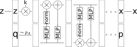
With the flow described above we can construct a TSF by choosing $p_{A}^{\tau}(\vec{q})=\mathcal{N}(\vec{q}|0,\tau)$ and choosing a dynamics $D$ with a constant Jacobian which satisfies the temperature scaling condition (Eq. 4). A convenient way of constructing volume preserving dynamics, i.e. $\left|\det J_{D}(\vec{\upsilon})\right|=1$, is obtained by altering the RNVP network structure [4], such that the product of the outputs of the scaling layers is equal to unity. This is done by subtracting the mean of the log outputs from each scaling layer, similar to [18]. In addition to the volume preserving RNVP layers we scale the latent space coordinates by a trainable scalar, which allows to adjust for entropy difference between the prior and the target. The resulting Jacobian factor is a constant and, hence, still fulfills the scaling condition. The flow architecture is shown in Fig. 1.

This architecture can also be viewed as an instance of an ANF, where the augmented prior distribution $p_{\Upsilon}^{\tau}\left(\vec{\upsilon}\right)=p_{Z}^{\tau}(\vec{z})p_{A}^{\tau}(\vec{q})$ is mapped to the joint output distribution $p_{\Gamma}^{\tau}\left(\vec{\gamma}\right)$ via the invertible dynamics $D.$ The joint target distribution is given by $\mu_{X}^{\tau}(\vec{x})p_{A}^{\tau}(\vec{p})$. As the flow fulfills the temperature scaling condition, a temperature change of the prior, i.e. $\tau\to\tau^{\prime}$, will change the output accordingly. In the case of a factorized output distribution $p_{\Gamma}^{\tau}\left(\vec{\gamma}\right)=p_{X}^{\tau}\left(\vec{x}\right)p_{A}^{\tau}\left(\vec{p}\right)$ the marginal distribution $p_{X}^{\tau}\left(\vec{x}\right)$ is scaled correctly as well. This is ensured if the joint target distribution is matched correctly.

Training

As in [14], the TSFs are trained by a combination of a maximum-likelihood (forward KL) and energy-based (reverse KL) loss $\mathcal{L}=\left(1-\lambda\right)\mathcal{L}_{ML}+\lambda\mathcal{L}_{KL}$, where the mixing parameter $\lambda$ is increased from zero during training. The maximum likelihood loss minimizes the negative log likelihood (nll), which requires samples from a distribution $p^{\prime}_{\Gamma}(\gamma)$ that is similar to the target distribution

$$\mathcal{L}_{ML}=\mathbb{E}_{\vec{\gamma}\sim p^{\prime}_{\Gamma}(\vec{\gamma})}\left[-\log p_{\Upsilon}(D^{-1}(\vec{\gamma}))-\log\left|\det J_{D^{-1}}(\vec{\gamma})\right|\right]$$ (5)

As the target energy $U(x)$ is defined by the physical system of interest, we can also rely on energy-based training where the reverse KL divergence is minimized via the variational free energy

$$\mathcal{L}_{KL}=\mathbb{E}_{\vec{\upsilon}\sim p_{\Upsilon}(\vec{\upsilon})}\left[U(D(\vec{\upsilon}))-\log\left|\det J_{D}(\vec{\upsilon})\right|\right]$$ (6)

Sampling and latent Monte Carlo

One way to generate samples using the TSF is by directly sampling from the Gaussian prior at the desired temperature and transforming the samples to configuration space. As the TSF is only an approximation to the Boltzmann distribution, these samples will generally be biased.

In order to ensure that the TSF generates unbiased samples from (2), we use it in a MCMC framework. A proposal $\vec{x}^{\prime}$ is generated from configuration $\vec{x}$ by sampling auxiliary momenta $\vec{p}\sim p_{A}^{\tau}\left(\vec{p}\right)$ to define $\vec{\gamma}=(\vec{x},\vec{p})$, then applying the inverse dynamics $\vec{\upsilon}=D^{-1}(\vec{\gamma})$ followed by a random displacement $\vec{\upsilon}^{\prime}=\vec{\upsilon}+\vec{\xi}$, with $\vec{\xi}\sim\mathcal{N}(0,\sigma^{2})$, in latent space and then transforming back into configuration space $(\vec{x}^{\prime},\vec{p}^{\prime})=D(\vec{\upsilon}^{\prime})$. Accepting such a step with acceptance probability $p_{\text{acc}}^{\tau}\left((\vec{x},\vec{p})\to(\vec{x}^{\prime},\vec{p}^{\prime})\right)=\min\left\{1,\exp\left[-\left(U(\vec{x}^{\prime})-U(\vec{x})+\left\|\vec{p}^{\prime}\right\|^{2}/2-\left\|\vec{p}\right\|^{2}/2\right)/\tau\right]\right\}$ enforces detailed balance in configuration space and thus ensures convergence to the Boltzmann distribution.

As the TSF is able to generate distributions at several temperatures, we can combine the MCMC moves with PT [19, 6, 9]. In PT, sampling is performed at a set of temperatures in parallel. Additionally to TSF-MCMC steps, samples can randomly be exchanged between two randomly chosen temperatures. This allows the sampler to overcome energy barriers quickly at high temperatures while still preserving details of the wells at lower temperatures.

3 Experiments

We carry out experiments at two different test models. Firstly, we demonstrate that the TSF drastically improves the temperature scaling as compared to the original RNVP. In a second experiment we show that for the Ala2 molecule the TSF is able to generate samples close to the Boltzmann distribution and that the MCMC scheme results in unbiased samples.

Mixture of multi-dimensional double wells

Figure 2: Results for the multi-dimensional double well system. A: marginal density of the first 5 coordinates of the 20d system. B: comparison of the nll as a function of the temperature between the TSF and the RNVP network structure in the 5 dimensional case (lower is better). The dashed line indicates the training temperature $T=1$ C: same as B but for the 20 dimensional system.

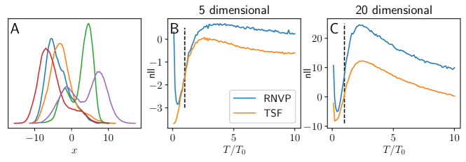
As a toy system that can easily be formulated in different dimensions, we select a mixture of multi-dimensional double wells which are mixed via a correlation matrix. The energy of this system is given by $U(x)=U_{\text{dw}}(A\vec{x}),$ with $U_{\text{dw}}(\vec{x})=\sum_{i}^{d}a_{i}x_{i}+bx_{i}^{2}+cx_{i}{}^{4}$. The parameter vector $\vec{a}$ and correlation matrix $A$ are chosen at random. We study the system at dimensions $d=\{5,20\}$ and compare the TSF with a RNVP flow with comparable numbers of trainable parameters. Fig. 2 left shows the marginal density of the first 5 coordinates of the 20d system. The Boltzmann Generators are trained at $T=1$ and then analyzed by comparing the nll (Eq. 5) of equilibrium samples, which were generated by Gaussian increment MCMC in combination with PT at $100$ temperatures in the range $T=0.1$ to $T=10$ (Fig. 2 center and right). For the 5d system we observe that both network structures perform equally well in the close vicinity of the training temperature, however the TSF has a significantly lower nll at temperatures further away from the ones it was trained on. In the case of the 20d system, the TSF consistently outperforms the RNVP even at the training temperature. This indicates that the TSF is a more expressive network structure with stronger temperature scaling.

Alanine Dipeptide

Figure 3: Results for Alanine Dipeptide (D) in implicit solvent. A, B, E, F: Density of $\phi,\psi$ variables from different methods. A: TSF samples generated at the training temperature of $T=600$ K (ground truth is B). E: Samples generated with the same TSF at $T=300$ K to be compared (ground truth is F). Histograms of the dihedral angle $\phi$ are shown in C for $T=600$ K and in G for $T=300$ K. H: Energy histograms at the different temperatures. D: Alanine Dipeptide molecule

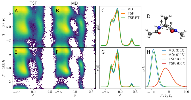
We further test TSF on the Alanine Dipeptide molecule in an implicit solvent model. For this system we use an invertible coordinate transformation layer and operate the TSF on a representation of the molecule in terms of distances and angles. As we are specifically interested in the temperature scaling aspect, we generate sets of samples at temperatures $T=\{300\>\mathrm{K},600\>\mathrm{K}\}$ using MD. Our goal is to use the samples at $T=600\>\mathrm{K}$ to train the TSF and then use the TSF to sample at $T=300\>\mathrm{K}$. The MD set at $T=300\>\mathrm{K}$ serves as ground truth for comparison. We use the TSF to generate samples in configuration space and compare the Ramachandran plots and distributions of the $\phi$ angle (Fig. 3). We observe good agreement at the training temperature (Fig. 3 panels A to C). At $T=300\>\mathrm{K}$ (Fig. 3 panels E to G) the TSF still finds the major minima at around $\phi\approx-2$, but under-samples the minimum at $\phi\approx 1$. This deviation from the target distribution is likely stemming from limited expressivity of the flow. We are able to recover the correct distribution of $\phi$ when using the Monte Carlo scheme in a PT fashion (Fig. 3 C and G). Furthermore, the output of the TSF closely recovers the distribution of energies (Fig. 3 H) at both temperatures.

4 Discussion

In this work, we derived and constructed temperature-steerable flows (TSF) that correctly scale the output distribution of a BG with temperature. We showed that this novel type of flow can be used to train a BG at one temperature and generate distributions at other temperatures. Further progress could be made by combining samples at different temperatures when collecting training data and thus improve the quality of the BG. Another application could be the investigation of temperature dependent observables, e.g. magnetization in spin systems or free energy difference in proteins.

5 Broader impact

Sampling equilibrium samples is important for physics and other fields. Applications range from development of new materials to drug discovery. A lot of computational resources and energy is required for these simulations. Enhancing such sampling algorithms with Machine Learning methods has the potential to increase the efficiency. Allowing to reduce the computational cost and thus energy consumption significantly. One promising approach to tackle this problem are the framework of Boltzmann Generators (BGs), to which this paper contributes. This paper enables BGs to generate Boltzmann Distributions at different temperatures. This allows them to be trained at high temperatures where sampling is comparably cheap and furthermore to be used in enhanced sampling algorithms such as parallel tempering.

One risk of this method is that enabling and improving sampling methods for which currently no convergence criterion is known can lead to false claims. In the context of flow bases samplers ergodicity is not well studied. While broken ergodicity can also be an issue in MD and MCMC, these are known to be ergodic at least in the asymptotic limit, i.e. the limit of infinitely long simulations. This needs to be further researched to arrive at criteria that guarantee convergence.

6 Acknowledgments

We gratefully acknowledge support by the Deutsche Forschungsgemeinschaft (SFB1114, project C03), the European research council (ERC CoG 772230 “ScaleCell”), the Berlin Mathematics center MATH+ (AA1-6), and the German Ministry for Education and Research (BIFOLD - Berlin Institute for the Foundations of Learning and Data). We thank Jonas Köhler, Andreas Krämer and Yaoyi Chen for insightful discussions.

References

- [1] MS Albergo, G Kanwar, and PE Shanahan. Flow-based generative models for markov chain monte carlo in lattice field theory. Physical Review D, 100(3):034515, 2019.
- [2] D. Boyda, G. Kanwar, Sébastien Racanière, Danilo Jimenez Rezende, M. S. Albergo, K. Cranmer, D. Hackett, and P. Shanahan. Sampling using SU(N) gauge equivariant flows. ArXiv, abs/2008.05456, 2020.
- [3] L. Dinh, D. Krueger, and Y. Bengio. Nice: Nonlinear independent components estimation. arXiv:1410.8516, 2015.
- [4] Laurent Dinh, Jascha Sohl-Dickstein, and Samy Bengio. Density estimation using real nvp. arXiv preprint arXiv:1605.08803, 2016.
- [5] Simon Duane, Anthony D Kennedy, Brian J Pendleton, and Duncan Roweth. Hybrid monte carlo. Physics letters B, 195(2):216–222, 1987.
- [6] Charles J. Geyer. Markov chain monte carlo maximum likelihood. In Proceedings of the 23rd Symposium on the Interface, pages 156–163, 1991.
- [7] Samuel Greydanus, Misko Dzamba, and Jason Yosinski. Hamiltonian neural networks. In Advances in Neural Information Processing Systems, pages 15379–15389, 2019.
- [8] C. Huang, Laurent Dinh, and Aaron C. Courville. Augmented normalizing flows: Bridging the gap between generative flows and latent variable models. ArXiv, abs/2002.07101, 2020.
- [9] K. Hukushima and K. Nemoto. Exchange monte carlo method and application to spin glass simulations. Journal of the Physical Society of Japan, 65:1604–1608, 1996.
- [10] Ivan Kobyzev, Simon Prince, and Marcus Brubaker. Normalizing flows: An introduction and review of current methods. IEEE Transactions on Pattern Analysis and Machine Intelligence, 2020.
- [11] Jonas Köhler, Leon Klein, and F. Noé. Equivariant flows: exact likelihood generative learning for symmetric densities. ArXiv, abs/2006.02425, 2020.
- [12] S. Li and Lei Wang. Neural network renormalization group. Physical review letters, 121 26:260601, 2018.
- [13] Kim A. Nicoli, Shinichi Nakajima, Nils Strodthoff, W. Samek, K. Müller, and P. Kessel. Asymptotically unbiased estimation of physical observables with neural samplers. Physical review. E, 101 2-1:023304, 2020.
- [14] Frank Noé, Simon Olsson, Jonas Köhler, and Hao Wu. Boltzmann generators-sampling equilibrium states of many-body systems with deep learning. Science, 365:eaaw1147, 2019.
- [15] George Papamakarios, Eric T. Nalisnick, Danilo Jimenez Rezende, Shakir Mohamed, and Balaji Lakshminarayanan. Normalizing flows for probabilistic modeling and inference. ArXiv, abs/1912.02762, 2019.
- [16] D. J. Rezende and S. Mohamed. Variational inference with normalizing flows. arXiv:1505.05770, 2015.
- [17] Danilo Jimenez Rezende, Sébastien Racanière, Irina Higgins, and Peter Toth. Equivariant hamiltonian flows. arXiv preprint arXiv:1909.13739, 2019.
- [18] P. Sorrenson, C. Rother, and U. Köthe. Disentanglement by nonlinear ICA with general incompressible-flow networks (GIN). ArXiv, abs/2001.04872, 2020.
- [19] Robert H Swendsen and Jian-Sheng Wang. Replica monte carlo simulation of spin-glasses. Physical review letters, 57(21):2607, 1986.
- [20] Esteban G. Tabak and Eric Vanden-Eijnden. Density estimation by dual ascent of the log-likelihood. Commun. Math. Sci., 8:217–233, 2010.
- [21] Peter Toth, Danilo Jimenez Rezende, Andrew Jaegle, Sébastien Racanière, Aleksandar Botev, and Irina Higgins. Hamiltonian generative networks. ArXiv, abs/1909.13789, 2019.
- [22] H. Wu, Jonas Köhler, and F. Noé. Stochastic normalizing flows. ArXiv, abs/2002.06707, 2020.
- [23] Linfeng Zhang, Lei Wang, et al. Monge-Ampère flow for generative modeling. arXiv preprint arXiv:1809.10188, 2018.