Abstract

The unprecedented coronavirus disease 2019 (COVID-19) pandemic is still a worldwide threat to human life since its invasion into the daily lives of the public in the first several months of 2020. Predicting the size of confirmed cases is important for countries and communities to make proper prevention and control policies so as to effectively curb the spread of COVID-19. Different from the 2003 SARS epidemic and the worldwide 2009 H1N1 influenza pandemic, COVID-19 has unique epidemiological characteristics in its infectious and recovered compartments. This drives us to formulate a new infectious dynamic model for forecasting the COVID-19 pandemic within the human mobility network, named the SaucIR-model in the sense that the new compartmental model extends the benchmark SIR model by dividing the flow of people in the infected state into asymptomatic, pathologically infected but unconfirmed, and confirmed. Furthermore, we employ dynamic modeling of population flow in the model in order that spatial effects can be incorporated effectively. We forecast the spread of accumulated confirmed cases in some provinces of mainland China and other countries that experienced severe infection during the time period from late February to early May 2020. The novelty of incorporating the geographic spread of the pandemic leads to a surprisingly good agreement with published confirmed case reports. The numerical analysis validates the high degree of predictability of our proposed SaucIR model compared to existing resemblance. The proposed forecasting SaucIR model is implemented in Python. A web-based application is also developed by Dash (under construction).

Key words:   asymptomatic transmission; compartmental model; forecasting; human mobility network

1 Introduction

The conventional susceptible-infected-recovered (SIR) dynamic model is one of the simplest compartmental models in epidemiology that segments the flows of people into three states, i.e., susceptible (S), infected (I), and resistant/recovered (R). The SIR model is used to compute the theoretical number of people infected with a contagious illness in a closed population over time [Kermack(1927)]. It has been widely applied and expanded to estimate or to predict the spread size of contagion phenomena such as the worldwide 2009 H1N1 influenza pandemic and severe acute respiratory syndrome (SARS) in 2003 for the purpose of infection prevention and control and public health strategies [Brockmann(2013)]. Modeling dynamics of coronavirus disease 2019, COVID-19 in short, remains a big challenge, although there has been sporadic investigation in the past few months [Hao(2020)]. The goal of this project is to to develop an expansion of the SIR model, named SaucIR, in response to the spread of the COVID-19 pandemic on the basis of its specific epidemiological characteristics and dynamic migration.

Unfortunately, the officially deployed interventions based on the SIR model were invalidated at the outbreak of COVID-19, particularly at the early stage when COVID-19 burst onto the global pandemic scene, even though the SARS 2003 epidemic and COVID-19 share many similarities. According to the editorial of New England Journal of Medicine (NEJM) in April 2020, the rapid, worldwide spread of COVID-19 resulted in more than 2.6 million people infected within five months, in contrast to the fact that SARS 2003 was controlled within 8 months with less than ten thousand persons infected in limited geographic areas [Gandhi(2020)]. More worldwide dynamic data of the infection spread are available to the public [Infection]. There are quite a few key factors to interpret the dramatically different trajectories of transmission and spread between COVID-19 and SARS 2003. For instance, one epidemiological key influence factor is the existence of asymptomatic individuals, who are the silent carriers of coronavirus. Such asymptomatic infections were diagnosed with positive RT-PCR test results but without any relevant clinical symptoms in the preceding days or during hospitalization, inducing the risk of spreading the disease and hence preventing ascertainment before symptoms [Gandhi(2020)]. Therefore, symptom-based detection of infection is less effective in COVID-19, compared to influenza and the SARS 2003 epidemic [To(2020)]. To examine asymptomatic transmission is necessary to fully consider in forecasting the spread size of the COVID-19 pandemic for effective public health prevention and control.

Driven by the nonignorable presence of asymptomatic transmission of the COVID-19 disease, we present a new dynamic model for the spread of infection by partitioning the infectious compartment of the traditional SIR model into three parts, i.e., asymptomatic cases, pathologically infected but unconfirmed cases, and confirmed cases.

Another crucial factor is dynamic human mobility in formulating the spread of the COVID-19 pandemic, driven by the effectiveness of isolating the spread of COVID-19 through lockdown of Wuhan city before the Chinese Spring Festival. The key initiative of such an extreme public health intervention ahead of major public holidays was to cut off the massive human movement between Wuhan and surrounding cities. The spread of virus was controlled, with evidence that the reproductive number $R_{t}$ decreased over time $t$, by 2.7-3.8 before January 26 to less than 1.0 after February 6, and less than 0.3 after March 1 [Pan(2020)]. This encourages us to incorporate dynamic spreading patterns within the spatial framework of the human mobility network [Brockmann(2013)]. The predictability of the spread of infectious disease could be improved by characterizing the geographical spread of epidemics [Rvachev(1985), Hufnagel(2004)]. Population flowing out of Wuhan has been incorporated to predict the risk and distribution of confirmed cases spatially [Jia(2011)]. Geographical dispersion of an epidemic through human mobility has also been successfully applied to forecast the spreading of SARS 2003 and H1N1 2009 [Brockmann(2013)], whereas the mobility parameter was fixed as a constant on all nodes. Such constant mobility assumption is reasonable for SARS 2003 but not applicable for COVID-19 because the latter infectious disease is more contagious and there is much more intense human mobility in 2020 compared to 13 years ago [Callaway(2020)].

In expanding the SIR model to our proposed SaucIR model, our main concerns focus on two aspects: (1) the division of infectious compartment into three separate segments, and (2) dynamic human mobility by separating the group size of migration in and out of a node within a network. It improves the prediction fidelity as shown in our simulation results. Furthermore, we demonstrate that it is possible to control the confirmed cases by reducing aggregation of migration among nodes in the human mobility network.

The remainder is organized as below. In Section 2, we give the formulation of the new SaucIR model for the spread of COVID-19 based on its epidemiological characteristics and dynamic geographical spread. We present a practical way to measure dynamic human mobility and suggest optimal enhancement for public control strategies. In Section 3, we apply the SaucIR model to estimate and predict the confirmed cases in mainland China and in worldwide countries with severe infections. In Section 4, we assess the predictive accuracy by comparing the proposed and the existing resembling models.

2 Formulation of new spread model of COVID-19

In this section, we formulate the predictive spread model of COVID-19 involving key factors driven from the epidemiological characteristics such as asymptomatic cases and dynamic human mobility within a network of coupled populations. We start from the following dynamics model [Brockmann(2013)] describing the local disease time course on each node based on the conventional SIR model:

$$\begin{split}&\partial_{t}S_{n}=-\frac{\alpha I_{n}S_{n}}{N_{n}},\\ &\partial_{t}I_{n}=\frac{\alpha I_{n}S_{n}}{N_{n}}-\beta_{0}I_{n},\end{split}\qquad n=1,\dots,M,$$ (2.1)

where $S_{n}$ and $I_{n}$ represent the numbers of susceptible and infected individuals on node $n$ in a network of people flow with a total of $M$ nodes, respectively, $N_{n}$ is the population size of node $n$, $R_{n}=N_{n}-S_{n}-I_{n}$ represents the number of recovered or deceased on node $n$, $\alpha$ is the mean infection rate of individuals, $\beta_{0}$ is the mean recovery rate of individuals, and $\partial_{t}X_{n}$ stands for the partial derivative of the population size of state $X$ on node $n$ with respect to time $t$ in a time course with $X$ being the place holder for $S$, $I$, or any other disease state alphabet in the modeling thereafter. The epidemiological threshold $R_{0}=\alpha/\beta$ is an indication of the transmissibility of a virus, governing the time evolution of the aforementioned equations.

2.1 Segmenting the infectious compartment

One of the epidemiological characteristics of COVID-19 that is remarkably different from existing infectious diseases such as SARS is the existence of asymptomatic carriers. Hence, symptom-based screening alone failed to detect a high proportion of infectious cases for asymptomatic persons and was not enough to control transmission. The probable asymptomatic transmission will not be known for sure unless an antibody test is applied. The risk of asymptomatic transmission cannot be ignored because of a large number of asymptomatic carriers [Mizumoto(2020), Bai(2020), Lee(2020)]. Thus, it is reasonable to segment the asymptomatic infected COVID-19 carriers independently in the infectious compartment. As a result, the infectious compartment is partitioned into two segments, i.e., the asymptomatic ($A$) and the symptomatic. Additionally, the symptomatic segment exposes to dynamic process and is stratified into two stages, i.e., pathologically infected but unconfirmed ($U$) and confirmed ($C$). That is, the infectious group first experiences the onset of symptoms, then it may be confirmed clinically after a time lag, called the incubation period. Thereafter, the confirmed group will be isolated for therapy in the hospital and lose its transmissibility. The incubation period is contagious in our compartmental model [Li(2020)], which is in line with the existing assumption for modeling the spread of the SARS epidemic [Chowell(2003)]. The infectivity during the incubation period for COVID-19 is critical for controlling the disease [Liu(2020)]. As a result of the newly segmented infectious compartment, the $R$ (recovered or deceased) compartment composes of two parts, recovered or deceased ($R_{1}$) from the symptomatic compartment or recovered ($R_{2}$) from the asymptomatic compartment accordingly. The formulated contagion pattern is summarized in Figure 1 to illustrate the spread dynamics.

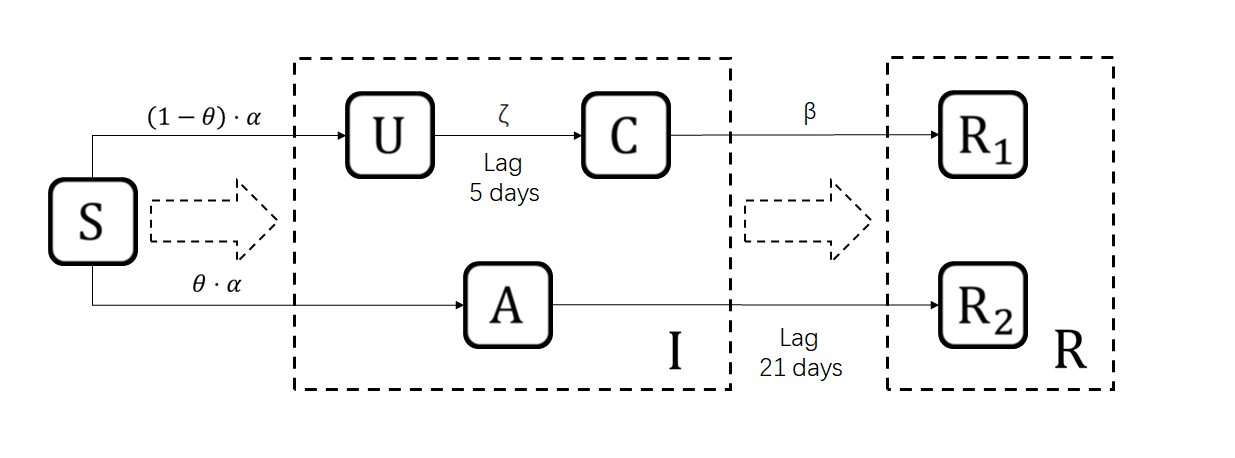
Figure 1: Progression flow of COVID-19. The parameters within the figure are illustrated in the adjacent paragraph.

Next, we analyze the key epidemiological parameters in Figure 1. The parameter $\alpha$ denotes the transmission rate from susceptible to infected, $\theta$ denotes the probability that susceptible individuals turn to be asymptomatically infected, $\zeta$ denotes the rate that a person in the incubation period turns to be confirmed clinically, and $\beta$ denotes the recovery rate from symptomatically confirmed to recovered or deceased. For the symptomatic segment, the time lag from $U$ to $C$ is taken as 5 days, the average incubation period in the literature [Lauer(2020)]. Our simulations show that the incubation period of 3 to 5 days is not sensitive to the proposed model. For the progression from asymptomatic ($A$) to recovered ($R_{2}$), the time lag 21 days corresponds to the maximal observation of the communicable period of asymptomatic carriers, counted from the first day of positive nucleic acid test to the first day of the continuous negative tests of an asymptomatic carrier [Bai(2020)]. There are very few references for the interval length of the communicable period of asymptomatic carriers to the pandemic spread [Hu(2020)]. Our simulation results show that the scope of 9-21 days will not affect much of the accuracy of the proposed model in Section 3.1. The aforementioned consideration of epidemiological characteristics is summarized in the following compartmental model on node $n$,

$$\begin{split}&\partial_{t}S_{n}=-\frac{\alpha_{n}(U_{n}+A_{n})S_{n}}{N_{n}},\\ &\partial_{t}U_{n}=\frac{\alpha_{n}(U_{n}+A_{n})S_{n}}{N_{n}}(1-\theta)-\zeta_{n}U_{n}^{t-5},\\ &\partial_{t}A_{n}=\frac{\alpha_{n}(U_{n}+A_{n})S_{n}}{N_{n}}\theta-A_{n}^{t-21},\\ &\partial_{t}C_{n}=\zeta_{n}U_{n}^{t-5}-\beta_{n}C_{n},\\ &\partial_{t}R_{1n}=\beta_{n}C_{n},\\ &\partial_{t}R_{2n}=A_{n}^{t-21},\qquad n=1,\dots,M,\end{split}$$ (2.2)

where $A_{n}$ represents the group size of asymptomatic cases, $U_{n}$ and $C_{n}$ are group sizes of infected but not yet confirmed clinically and confirmed clinically in the symptomatic segment, respectively, $R_{1n}$ and $R_{2n}$ denote the removed cases from symptomatic and asymptomatic segments, respectively, $\alpha_{n}$ denotes the average infection rate for population $n$ in the network, $\beta_{n}$ denotes the average recovery rate of individuals from confirmed clinically under therapy to recovered on node $n$, and $R_{1n}=N_{n}-S_{n}-(U_{n}+A_{n}+C_{n})-R_{2n}$.

Notice that for population $n$ in a network, the accumulated confirmed cases, denoted as $D$, is the sum of the clinically confirmed under therapy ($C$) and the recovered or deceased from symptomatic cases ($R_{1}$). Thereafter,

$$\partial_{t}D_{n}=\zeta_{n}U_{n}^{t-5}$$ (2.3)

will replace the bi-interrelated variation equations in the system of equations (2.2) in the final dynamic model.

2.2 Dynamic human mobility

We now incorporate the impact of population flow onto the modeling of the infectious spread of COVID-19. To guarantee the prediction fidelity, we distinguish the group size of people emanating from a node $m$ in and out of another node $n$, and hence, the distinct human mobility rates of moving in and out of a node $n$. This is a quite practical strategy considering the difference among nodes. Let $X$ be a placeholder for the compartments $S$, $U$, and $A$. The infection variation for population $n$ comes from two sources, local and migration,

$$\partial_{t}X_{n}=\partial_{t}X_{n,\textrm{local}}+\partial_{t}X_{n,\textrm{migration}},$$ (2.4)

where the first summand $\partial_{t}X_{n,\textrm{local}}$ on the right side of equation (2.4) represents the dynamic local disease time course on node $n$ by equations (2.2) and (2.3). Next, we will elucidate the formulating of $\partial_{t}X_{n,\textrm{migration}}$ based on parameters of dynamic human mobility.

Let $F_{nm}$ be the group size of people emanating from node $m$ to node $n$. Denote $F_{n\cdot}=\sum_{m}F_{nm}$ and $F_{\cdot m}=\sum_{n}F_{nm}$. Let $\gamma^{\textrm{in}}_{n}=F_{n\cdot}/N_{n}$ be the proportion of the group size moving in destination $n$ ($F_{n\cdot}$) to the population size of node $n$ ($N_{n}$), and $\gamma^{\textrm{out}}_{n}=F_{\cdot n}/N_{n}$ be the proportion of group size of people leaving node $n$ ($F_{\cdot n}$) to the population size of node $n$. Let $P^{\textrm{{in}}}_{nm}=F_{nm}/F_{n\cdot}$ be the proportion of group size emanating from node $m$ in destination $n$ to the group size moving in destination $n$; let $P^{\textrm{out}}_{mn}=F_{mn}/F_{\cdot n}$ be the proportion of group size leaving node $n$ for another node $m$ to the group size emanating from node $n$. Let $P_{nn}^{\textrm{{in}}}=0=P_{nn}^{\textrm{out}}$. Under the setting of such human mobility measurements, the variation of the susceptible within our spread model of COVID-19 satisfies

$$\begin{split}&\partial_{t}S_{n,\textrm{migration}}=\\ &\sum_{m=1}^{M}\bigg{[}\gamma_{n}^{\textrm{{in}}}P_{nm}^{\textrm{{in}}}S_{m}-\gamma_{n}^{\textrm{{in}}}P_{nm}^{\textrm{{in}}}\frac{\alpha_{m}(U_{m}+A_{m})S_{m}}{N_{m}}\\ &\quad\quad-\gamma_{n}^{\textrm{out}}P_{mn}^{\textrm{out}}S_{n}\bigg{]}.\\ \end{split}$$ (2.5)

Notice that, when there is no geometrical difference in transmission, denoted as $\gamma^{\textrm{{in}}}_{n}=\gamma^{\textrm{out}}_{n}\equiv\gamma$ for any node $n$, and there is no infection during the migration, denoted as $\alpha_{m}=0$, our proposed equation (2.5) reduces to the representation of $\partial_{t}S_{n}$ in the literature [Brockmann(2013)].

For $U_{n}$ and $A_{n}$, one cannot ignore the infection owing to human mobility among nodes in the geometrical network. The correspondent dynamic processes can be presented as follows:

$$\begin{split}&\partial_{t}U_{n,\textrm{migration}}\\ =&\sum_{m=1}^{M}\bigg{[}\gamma_{n}^{\textrm{{in}}}P_{nm}^{\textrm{{in}}}U_{m}+\gamma_{n}^{\textrm{{in}}}P_{nm}^{\textrm{{in}}}\frac{\alpha_{m}(1-\theta)(U_{m}+A_{m})S_{m}}{N_{m}}\\ &\quad\quad-\gamma_{n}^{\textrm{out}}P_{mn}^{\textrm{out}}U_{n}\bigg{]},\\ &\partial_{t}A_{n,\textrm{migration}}\\ =&\sum_{m=1}^{M}\bigg{[}\gamma_{n}^{\textrm{{in}}}P_{nm}^{\textrm{{in}}}A_{m}+\gamma_{n}^{\textrm{{in}}}P_{nm}^{\textrm{{in}}}\frac{\alpha_{m}\theta(U_{m}+A_{m})S_{m}}{N_{m}}\\ &\quad\quad-\gamma_{n}^{\textrm{out}}P_{mn}^{\textrm{out}}A_{n}\bigg{]},\end{split}$$ (2.6)

where $\alpha_{m}$ denotes the rate of infection at node $m$ other than node $n$.

Based on the spirit of equation (2.4), we can further update the dynamic model (2.2) by combining (2.3), (2.5), and (2.6) into (2.2).

2.3 The SaucIR-model

To formulate the final SaucIR model, we still need to further refine some nested parameters to enhance predictivity. In a network, the prevention and control policies of different nodes should lead to spatially varying epidemic parameters.

First of all, we will add the effects of quarantine into the modeling of the contagion pattern of COVID-19 [Chowell(2003)]. In mainland China, during the COVID-19 pandemic, most provinces have announced officially the detailed confirmed cases and labeled whether the specific case was once quarantined. This information is beneficial for estimating the quarantine rate parameter $l_{n}$ as the ratio of the size of quarantine labeled cases against the total number of confirmed cases of COVID-19 disease for population $n$. Still in modeling the spread of SARS by the literature [Chowell(2003)], $l_{n}$ changes over time. Varying $l_{n}$ is effective in the situation where there exist inflection points, validated by Figure 4 in literature [Chowell(2003)], whereas it is not significant for our proposed model, as confirmed by the simulations summarized in Table 11 and Figure 3.

The other focus of our study is the correction of the transmission rate $\alpha_{m}$ for the migration process. The transmission rate function is no doubt time and nodal dependent. Let $\tau_{n}$ be a decay constant on node $n$. The general exponential tilt expression

$$\alpha_{n}(t)=\alpha_{n}(0)\cdot e^{-\tau_{n}t}$$ (2.7)

is an acceptable functional to act in the local infectious process [Chen(2020)] in which the prevention and control in local governments can effectively help prevent the spread of contagion. However, the monotone decreasing function (2.7) is not suitable to apply in the migration process owing to unprecedented human mobility. Conservatively, we uniformly apply the nodal function $\alpha_{n}(t)$ to behave as the transmission rate function in the migration part of the final model.

All of the above considerations lead to the final SaucIR model illustrating the infection progression:

$$\begin{split}&\partial_{t}S_{n}=-(1-l_{n})\frac{\alpha_{n}(t)(U_{n}+A_{n})S_{n}}{N_{n}}\\ &\qquad\quad+\sum_{m=1}^{M}[\gamma_{n}^{\textrm{{in}}}P_{nm}^{\textrm{{in}}}S_{m}\\ &\qquad\quad-\gamma_{n}^{\textrm{{in}}}P_{nm}^{\textrm{{in}}}(1-l_{n})\frac{\alpha_{m}(0)(U_{m}+A_{m})S_{m}}{N_{m}}\\ &\qquad\quad-\gamma_{n}^{\textrm{out}}P_{mn}^{\textrm{out}}S_{n}],\\ &\partial_{t}U_{n}=(1-l_{n})\frac{\alpha_{n}(t)(U_{n}+A_{n})S_{n}}{N_{n}}(1-\theta)-\zeta_{n}U_{n}^{t-5}\\ &\qquad\quad+\sum_{m=1}^{M}[\gamma_{n}^{\textrm{{in}}}P_{nm}^{\textrm{{in}}}(1-l_{n})U_{m}\\ &\qquad\quad+\gamma_{n}^{\textrm{{in}}}P_{nm}^{\textrm{{in}}}(1-l_{n})\frac{\alpha_{m}(0)(1-\theta)(U_{m}+A_{m})S_{m}}{N_{m}}\\ &\qquad\qquad\qquad-\gamma_{n}^{\textrm{out}}P_{mn}^{\textrm{out}}(1-l_{n})U_{n}],\\ &\partial_{t}A_{n}=(1-l_{n})\frac{\alpha_{n}(t)(U_{n}+A_{n})S_{n}}{N_{n}}\theta-A_{n}^{t-21}\\ &\qquad\quad+\sum_{m=1}^{M}[\gamma_{n}^{\textrm{{in}}}P_{nm}^{\textrm{{in}}}(1-l_{n})A_{m}\\ &\qquad\quad+\gamma_{n}^{\textrm{{in}}}P_{nm}^{\textrm{{in}}}(1-l_{n})\frac{\alpha_{m}(0)\theta(U_{m}+A_{m})S_{m}}{N_{m}}\\ &\qquad\qquad\qquad-\gamma_{n}^{\textrm{out}}P_{mn}^{\textrm{out}}(1-l_{n})A_{n}],\\ &\partial_{t}D_{n}=\zeta_{n}U_{n}^{t-5},\\ &\partial_{t}R_{2n}=A_{n}^{t-21},\qquad n=1,\dots,M.\end{split}$$ (2.8)

The epidemic parameters $l_{n}$, $\alpha_{n}$, and $\zeta_{n}$ are estimated from the announced epidemic data by the provinces. The initial value of $S_{n}$ is the population size of every node. The initial value of $D_{n}$ is the number of cumulative confirmed cases each day. The initial value of $U_{n}$ is the sum of new diagnoses in the next six days. The initial value of $A_{n}$ is the total number of new diagnoses in the next six days multiplied by $\theta/(1-\theta)$.

2.4 Prevention and control strategy

In this subsection, we explore whether human mobility can be modified among nodes in a network to control or minimize the accumulated confirmed cases in a district over a certain time interval.

Let $D_{n}^{T}$ be the confirmed cases on node $n$ up to day $T$. Denote any local coupled populations in the network as $S=\{1,\cdots,K\}$, and all populations in the network as $S_{0}=\{1,\cdots,M\}$, where $K\leq M$. The migration-related parameters introduced before Section 2.3 on a specific day $t$ are then denoted as $\gamma_{n,t}^{\textrm{{in}}}$, $\gamma_{m,t}^{\textrm{out}}$, $P_{nm,t}^{\textrm{{in}}}$, and $P_{nm,t}^{\textrm{out}}$. The objective function will be optimized by choosing the appropriate time-dependent tuning parameters aforementioned.

Recall that we define $\gamma^{\textrm{in}}_{n}$, $\gamma^{\textrm{out}}_{n}$, $P^{\textrm{{in}}}_{nm}$, and $P^{\textrm{{out}}}_{mn}$, the parameters of the human mobility in a network, in Section 2.2. We add an extra suffix $t$ in the footnote to denote the corresponding parameters when time $t$ falls into the time interval $[0,T]$. Let $C_{nm,T}^{\textrm{{in}}}$ and $C_{nm,T}^{\textrm{out}}$ be the rate of emanating from node $m$ in and out to node $n$, respectively, in the network over the time period $[0,T]$. Then, it is readily seen that

$$\begin{split}&\sum_{t\in[0,T]}\gamma_{n,t}^{\textrm{{in}}}P_{nm,t}^{\textrm{{in}}}=C_{nm,T}^{\textrm{{in}}},\\ &\sum_{t\in[0,T]}\gamma_{m,t}^{\textrm{out}}P_{nm,t}^{\textrm{out}}=C_{nm,T}^{\textrm{out}},\ \forall m,n\in S_{0}.\ \ \end{split}$$ (2.9)

To modify parameters of human mobility among nodes in the network, for any pairwise nodes $n$ and $m$, one natural constraint is to keep a constant relationship between the group size emanating from node $n$ with population size $N_{n}$ and out of another node $m$ with population size $N_{m}$, so that the optimization problem may be presented as

$$\begin{split}&\min_{\gamma_{n,t}^{\textrm{{in}}},P_{nm,t}^{\textrm{{in}}},\gamma_{m,t}^{\textrm{out}},P_{nm,t}^{\textrm{out}}}\sum_{n\in S}D_{n}^{T}\text{ subject to }\\ &{C_{nm,T}^{\textrm{in}}N_{n}=C_{nm,T}^{\textrm{out}}N_{m},\ \forall m,n\in S_{0}.}\end{split}$$ (2.10)

For the optimization problem (2.10), we assume that the mobility group will not change the epidemic parameters $\alpha_{n}(t)$, $\beta_{n}$, $l_{n}$, and $\theta$ on node $n$. To solve the optimization problem (2.10), we employ the general genetic algorithm [Deb(1999)]. Here are notations involved in the algorithm. Denote $(\gamma P)^{\textrm{in}}_{nm,t}=\gamma_{n,t}^{\textrm{in}}P_{nm,t}^{\textrm{in}}$ and $(\gamma P)_{mn,t}^{\textrm{out}}=\gamma_{m,t}^{\textrm{out}}P_{nm,t}^{\textrm{out}}$; let $C_{T}^{\textrm{in}}$ and $C_{T}^{\textrm{out}}$ represent the matrices $(C_{nm,T}^{\textrm{in}})_{n,m\in S_{0}}$ and $(C_{nm,T}^{\textrm{out}})_{n,m\in S_{0}}$, respectively; and let $(\gamma P)^{\textrm{in}}$ and $(\gamma P)^{\textrm{out}}$ represent the three-dimensional matrices $((\gamma P)^{\textrm{in}}_{nm,t})_{t\in[0,T],n,m\in S_{0}}$ and $((\gamma P)_{mn,t}^{\textrm{out}})_{t\in[0,T],n,m\in S_{0}}$, respectively. The particular terminologies in the genetic algorithm and their correspondence in our problem are listed as below:

1. Individual: a matrix shaped as (T, M, M), where T and M correspond to $(\gamma P)^{\textrm{in}}_{nm,t}$ and $(\gamma P)_{mn,t}^{\textrm{out}}$, respectively, for $t\in[0,T]$ and $n,m\in S_{0}$.

2. Population: a collection of individuals.

3. Fitness: a description of how good an individual fits the environment, and in our study, how small the number of $\sum_{n}D_{n}^{T}$ is.

4. Selection, crossover, and mutation: specific operation in genetic algorithm, aiming to generate individuals that are more likely to correspond to better fitness.

Algorithm 1 provides the steps for minimizing the accumulated confirmed cases within any sub-network over a time interval, of which the function getfitness is presented in the following Algorithm 2.

Algorithm 1: minimize the accumulated confirmed cases
1: Initialize population
2: for iter = 1,$\ldots$, loop num do
3:  for individual in population do
4:   fitness(individual)=getfitness($C_{T}^{\textrm{in}}$,$C_{T}^{\textrm{out}}$,individual,$T$,$M$)
5:  end for
6:  record the best fitness so far
7:  selection(population, fitness)
8:  crossover(population)
9:  mutation(population)
10: end for

Algorithm 2: function getfitness implementing the SaucIR model
input: $C^{\textrm{in}}$, $C^{\textrm{out}}$, individual, $T$, $M$
1: set individual($t$, $m$, $m$)=0
2: for $m$ in range($M$) do
3:  for $n$ in range($M$) do
4:   summn=$\sum_{t}$(individual($t,m,n$))
5:   for $t$ in range($T$) do
6:    $(\gamma P)^{\textrm{in}}_{mn,t}$ = individual($t,m,n)C_{mn,T}^{\textrm{in}}$/summn
7:    $(\gamma P)^{\textrm{out}}_{mn,t}$ = individual($t,m,n$)$C_{mn,T}^{\textrm{out}}$/summn
8:   end for
9:  end for
10: end for
11: fitness=$-$equations (8)$((\gamma P)^{\textrm{in}},(\gamma P)^{\textrm{out}})$

Based on the SaucIR model (2.8), one may use Algorithms 1 and 2 to solve the minimization problem (2.10). Notice that the four tuning rate parameters are ratios among $F_{\cdot m}$, $F_{n\cdot}$, $N_{n}$, $N_{m}$, and $F_{nm}$. Therefore, governmental management may have a proper intervention on the migration size within a sub-network for the purpose of preventing and controlling the spread of COVID-19.

3 Numerical analysis and forecasting

In this section, we use the data of confirmed cases within the human mobility networks in mainland China and the international community to analyze the predictive fidelity of the SaucIR spread model (2.8) of COVID-19. To assess the accuracy of prediction, we adopt two assessment indices, max absolute percent error (MAPE) and root mean squared error (RMSE) with mathematical expressions

$$\text{MAPE}_{n}=\max_{t}\bigg{\{}\frac{|D_{n}^{\text{pred}}-D_{n}^{\text{real}}|}{D_{n}^{real}}\bigg{\}}$$

and

$$\text{RMSE}_{n}=\sqrt{\sum_{t}(D_{n}^{\text{pred}}-D_{n}^{\text{real}})^{2}/(t_{0}-1)},$$

respectively, where $t_{0}$ is the number of days of a prediction period with daily unity to count time, and the superscripts “pred” and “real” denote predicted and real, respectively. MAPE reflects the maximal daily percentage error out of the total number of infections over the forecasting time period, whereas RMSE measures the averaged headcount error over the forecasting time period. The prediction is more accurate with lower levels of such errors.

3.1 Analysis of human mobility network in mainland China

Table 1: MAPE assessing effect of asymptomatic infections spatially

	Province
$\theta$	Beijing	Shanghai	Jiangsu	Zhejiang	Anhui	Guangdong	Henan	Hunan	Chongqing	Sichuan	Jiangxi
0.05	0.033	0.033	0.028	0.019	0.008	0.032	0.008	0.018	0.012	0.023	0.025
0.15	0.013	0.021	0.019	0.017	0.006	0.009	0.004	0.022	0.009	0.008	0.004
0.25	0.017	0.006	0.015	0.011	0.006	0.015	0.005	0.014	0.009	0.009	0.010
0.35	0.015	0.006	0.014	0.006	0.005	0.015	0.003	0.003	0.005	0.007	0.017
0.45	0.015	0.006	0.019	0.009	0.001	0.028	0.011	0.012	0.003	0.005	0.012
0.55	0.026	0.021	0.011	0.029	0.007	0.047	0.008	0.009	0.012	0.023	0.028

Table 2: RMSE assessing effect of asymptomatic infections spatially

	Province
$\theta$	Beijing	Shanghai	Jiangsu	Zhejiang	Anhui	Guangdong	Henan	Hunan	Chongqing	Sichuan	Jiangxi
0.05	11	13	15	22	6	48	8	20	8	13	23
0.15	5	7	10	19	6	15	6	23	5	4	3
0.25	5	2	8	10	5	17	7	13	5	5	8
0.35	5	2	7	8	5	17	3	3	3	4	13
0.45	5	2	10	9	1	30	16	11	2	2	10
0.55	9	9	16	31	6	56	10	8	6	12	24

Table 3: MAPE assessing effect of different lag of days of incubation period

	Province
Lag (days)	Beijing	Shanghai	Jiangsu	Zhejiang	Anhui	Guangdong	Henan	Hunan	Chongqing	Sichuan	Jiangxi
3	0.018	0.006	0.019	0.008	0.008	0.017	0.012	0.021	0.018	0.010	0.026
4	0.016	0.006	0.017	0.007	0.007	0.008	0.010	0.002	0.002	0.004	0.010
5	0.018	0.006	0.016	0.011	0.006	0.015	0.006	0.015	0.009	0.010	0.011
6	0.015	0.012	0.029	0.004	0.012	0.011	0.006	0.007	0.007	0.019	0.012
7	0.043	0.024	0.021	0.016	0.021	0.012	0.029	0.016	0.016	0.041	0.016

Table 4: Range of uncertainty of MAPE assessing effect of [3,5] lag of days of incubation period

	Province
	Beijing	Shanghai	Jiangsu	Zhejiang	Anhui	Guangdong	Henan	Hunan	Chongqing	Sichuan	Jiangxi
Maximum	0.018	0.006	0.019	0.011	0.008	0.017	0.012	0.021	0.018	0.01	0.026
Mininum	0.016	0.006	0.016	0.007	0.006	0.008	0.006	0.002	0.002	0.004	0.01

Table 5: RMSE assessing effect of different lag of days of incubation period

	Province
Lag (days)	Beijing	Shanghai	Jiangsu	Zhejiang	Anhui	Guangdong	Henan	Hunan	Chongqing	Sichuan	Jiangxi
3	5	1	9	8	6	21	13	19	9	4	20
4	4	2	8	7	7	9	11	2	1	2	7
5	5	2	8	10	4	17	6	12	4	4	8
6	5	4	15	5	8	10	6	7	4	7	12
7	14	9	12	22	19	12	37	18	7	22	17

Table 6: Range of uncertainty of RMSE assessing effect of [3,5] lag of days of incubation period

	Province
	Beijing	Shanghai	Jiangsu	Zhejiang	Anhui	Guangdong	Henan	Hunan	Chongqing	Sichuan	Jiangxi
Maximum	5	2	9	10	7	21	13	19	9	4	20
Minimum	4	1	8	7	4	9	6	2	1	2	7

Table 7: MAPE assessing effect of different lag of days of the median communicable period

	Province
Lag (days)	Beijing	Shanghai	Jiangsu	Zhejiang	Anhui	Guangdong	Henan	Hunan	Chongqing	Sichuan	Jiangxi
21	0.018	0.006	0.016	0.011	0.006	0.015	0.006	0.015	0.009	0.01	0.011
18	0.015	0.015	0.021	0.006	0.007	0.004	0.006	0.008	0.011	0.019	0.008
15	0.02	0.018	0.013	0.003	0.012	0.004	0.013	0.001	0.013	0.014	0.003
12	0.018	0.021	0.014	0.013	0.007	0.009	0.004	0.008	0.016	0.014	0.003
9	0.018	0.012	0.016	0.003	0.012	0.01	0.009	0.016	0.011	0.012	0.013
6	0.02	0.006	0.035	0.017	0.016	0.025	0.034	0.015	0.02	0.016	0.021

Table 8: Range of MAPE assessing effect of [9,21] lag of days of the median communicable period

	Province
	Beijing	Shanghai	Jiangsu	Zhejiang	Anhui	Guangdong	Henan	Hunan	Chongqing	Sichuan	Jiangxi
Maximum	0.02	0.021	0.021	0.013	0.012	0.015	0.013	0.016	0.016	0.019	0.013
Minimum	0.015	0.006	0.013	0.003	0.006	0.004	0.004	0.001	0.009	0.01	0.003

Table 9: RMSE assessing effect of different lag of days of the median communicable period

	Province
Lag (days)	Beijing	Shanghai	Jiangsu	Zhejiang	Anhui	Guangdong	Henan	Hunan	Chongqing	Sichuan	Jiangxi
21	5	2	8	10	4	17	6	12	4	4	8
18	5	5	11	8	6	5	6	9	5	9	7
15	6	6	8	3	10	4	15	1	6	6	2
12	6	7	10	17	6	10	4	8	8	6	2
9	5	3	8	3	10	11	12	18	5	5	11
6	6	2	17	23	16	26	38	16	9	6	18

Table 10: Range of RMSE assessing effect of [9,21] lag of days of the median communicable period

	Province
	Beijing	Shanghai	Jiangsu	Zhejiang	Anhui	Guangdong	Henan	Hunan	Chongqing	Sichuan	Jiangxi
Maximum	6	7	11	17	10	17	15	18	8	9	11
Minimum	5	2	8	3	4	4	4	1	4	4	2

Table 11: MAPE assessing effect of the quarantine rate

	Province
$l_{n}$	Beijing	Shanghai	Jiangsu	Zhejiang	Anhui	Guangdong	Henan	Hunan	Chongqing	Sichuan	Jiangxi
0.4	0.016	0.012	0.021	0.011	0.01	0.011	0.007	0.012	0.004	0.016	0.011
0.5	0.02	0.015	0.019	0.003	0.006	0.013	0.008	0.016	0.011	0.012	0.013
0.6	0.016	0.006	0.021	0.009	0.01	0.019	0.007	0.014	0.004	0.012	0.008

We use epidemic and migration data from January 24 through February 15, 2020, to forecast confirmed case numbers on February 16-18, 2020, for a network of human mobility including 11 nodes (provinces) in mainland China. The spread of COVID-19 during the period kept on growing and did not reach a steady stage. The epidemic data is available through the link [Mainland-China-Infection]. Data sets of the migration part are obtained from the Baidu Migration [Migration]. This website provides the group size of people emanating from each province, and the percent of migration from one province to another province.

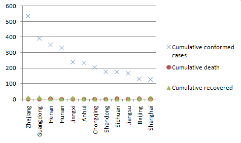
Figure 2: Cumulative numbers of diagnoses on January 30, 2020.

We choose 11 Chinese provinces that were the most severely infected nationally during the time period, excluding Shandong and Hubei. The epidemic data of Shandong province are not included in this study as the cumulative number of confirmed cases dropped unusually on a period of consecutive three days. Hubei province is not included in the analysis because of the Wuhan lockdown that went into effect on January 24, 2020, cutting off the population mobility from those outside the province. Figure 2 displays the cumulative numbers of epidemic data such as confirmed cases, deceased cases, and recovered cases of the top 11 severely infected provinces aforementioned on January 30, 2020. The cumulative number of diagnoses in Shanghai is not available in the previously mentioned data link but can be obtained from the Shanghai Municipal Health Commission [Shanghai-Infection-Data].

In the following analysis, we first evaluate the effects of components of the model and the sensitivity of parameters involved in the model. We then assess the prediction fidelity of the proposed SaucIR model and compare the prediction result based on the epidemic and migration data in mainland China.

Table 12: MAPE evaluation of prediction of confirmed cases China nationally

	Province
Method	Beijing	Shanghai	Jiangsu	Zhejiang	Anhui	Guangdong	Henan	Hunan	Chongqing	Sichuan	Jiangxi
SIR	0.036	0.018	0.015	0.007	0.026	0.035	0.016	0.017	0.014	0.038	0.041
SIR+M	0.039	0.024	0.012	0.007	0.026	0.036	0.015	0.016	0.014	0.038	0.041
SaucIR-M	0.018	0.006	0.023	0.011	0.016	0.021	0.007	0.021	0.019	0.015	0.016
SaucIR	0.017	0.006	0.015	0.011	0.006	0.015	0.005	0.014	0.009	0.009	0.010

Table 13: RMSE evaluation of prediction of confirmed cases China nationally

	Province
Method	Beijing	Shanghai	Jiangsu	Zhejiang	Anhui	Guangdong	Henan	Hunan	Chongqing	Sichuan	Jiangxi
SIR	16	5	8	7	23	45	21	15	7	21	36
SIR+M	16	7	7	7	23	47	21	14	7	21	36
SaucIR-M	6	2	15	11	13	24	9	20	12	8	13
SaucIR	5	2	8	10	5	17	7	13	5	5	8

Firstly, we evaluate the effects of the asymptomatic component in the SaucIR model, including the proportion of asymptomatic carriers and the communicable period of asymptomatic carriers. On one hand, we conduct simulations studying the effects of different levels of the rate of asymptomatic people ($\theta$) on the prediction accuracy. The results are summarized in Tables 1 and 2. The values of $\theta$ may be different spatially. Our simulation results assess and show that the SaucIR model works well when $\theta$ takes values between 0.15 to 0.45 in terms of MAPE and RMSE. Both MAPE and RMSE show a similar pattern, such that the measure error first decreases and then increases as $\theta$ varies starting from 0.05 and upward to 0.45. The bottom points of $\theta$ of measurement errors are slightly different among provinces. Thus, it may be concluded that $\theta$ affects the error of the predicted results but the prediction accuracy may be guaranteed when it is controlled under 0.45. Hence, we uniformly use 0.25 as the rate of the asymptomatic infected group to analyze the predictive fidelity of the proposed model. Another observation is that the supercity Beijing has relatively larger values of MAPE and RMSE, which are highly likely due to the relatively extensive amount of imported cases based on the news and media report. On the other hand, we validate it is reasonable to take 21 days as the communicable period of asymptomatic carriers. We conduct a sensitivity analysis to compare the effect of selecting different communicable period on the prediction accuracy. According to the literature [Hu(2020)], we select the length of time consisting of 6-21 days in the simulations. Both RMSE and MAPE reflect that the prediction error is smaller in most areas when the length of time varies between 9 and 21 (Tables 7 and 9), and the effect of the value on the prediction error is small (Tables 8 and 10).

Secondly, we evaluate the sensitivity of the incubation period in the symptomatic process. We conduct a sensitivity analysis to check whether the spread results change substantially for various incubation period. Considering the incubation period in the literature [Lauer(2020)], we take 3 to 7 days on the spread of the disease. Both RMSE and MAPE reflect that the incubation period corresponding to the best forecast varies from region to region. When the incubation period is between 3 and 5 days, the forecast error is small in most areas (Tables 3 and 5), and the effect of changing incubation period in this interval is small (Tables 4 and 6). Consequently, 5 days is acceptable uniformly.

Next, we use simulations to compare the effect of choosing different $l_{n}$. As mentioned in Section 2.3, it is reasonable to keep $l_{n}$ constant over time. Because there are no inflection points in Figure 3, and the gains from making $l_{n}$ change over time come mainly from the inflection point. We then use simulations to compare the effect of choosing different $l_{n}$ fixed with time. Since the estimated $l_{n}$ varies between 0.4 and 0.6 in the real data, we consider three values of $l_{n}$ (i.e., 0.4, 0.5, and 0.6) for each node. Both MAPE and RMSE show that the model is insensitive to the value of $l_{n}$ (Table 11).

Table 14: Predicted numbers of confirmed cases.

	Country
Date	Italy	Spain	German	USA	France	South Korea	UK
05.19.2020 (Pred)	225605	278216	177821	1548974	181245	10992	249210
05.19.2020 (Obs)	225886	278188	177289	1550294	180051	11078	247709
05.19.2020 (PE)	-0.0012	0.0001	0.003	-0.0009	0.0066	-0.0078	0.0061
05.20.2020 (Pred)	226315	279774	178518	1564915	181651	10994	252171
05.20.2020 (Obs)	226699	278803	178150	1570583	180934	11110	250141
05.20.2020 (PE)	-0.0017	0.0035	0.0021	-0.0036	0.004	-0.0104	0.0081
05.21.2020 (Pred)	226997	281281	179194	1580095	182035	10996	255017
05.21.2020 (Obs)	227364	279524	178748	1592723	181700	11122	252234
05.21.2020 (PE)	-0.0016	0.0063	0.0025	-0.0079	0.0018	-0.0113	0.011

Pred, predicted number; Obs, real number; PE, percentage error for every country.

Finally, we evaluate the prediction performance of our method through simulations. We demonstrate that the proposed segmentation of the infection compartment significantly improves the prediction accuracy and that the incorporation of dynamic human mobility apparently enhances the prediction accuracy. We use SIR+M to denote model (3) in the literature [Brockmann(2013)], and use SIR and SaucIR-M to denote models (2.1) (without further segmentation) and (2.2) (without dynamic human mobility) in Section 2.1, respectively. The comparison results are summarized in Tables 12 and 13. The predicted RMSE is in single digits except for Zhejiang, Guangdong, and Hunan.

Figure 3 shows the real numbers of confirmed cases and the fitted numbers of confirmed cases by SIR+M and our method during the period from January 24 to February 15, 2020, and forecast numbers of confirmed cases for the next three days. In both the SIR+M and our method, the real numbers of confirmed cases from January 24 to February 15, 2020 are used to estimate epidemic parameters. In most provinces, the forecast accumulated numbers of confirmed cases by SIR+M are generally larger than the real magnitudes. Our conjecture is, in SIR+M, the decrease of the transmission rate $\alpha$ is the main factor that affects the slowdown in the growth of the number of confirmed cases, whereas in SaucIR, the group sizes of the segments $U$ and $A$ will take effects simultaneously together with the transmission rate $\alpha$. Notice that, the partition of $I$ into $A$ and $U+C$ shown in Figure 1 implies that the size of the infectious compartment in SaucIR is smaller than that in SIR+M because the group of $C$ loses transmissibility owing to isolation for therapy. Also, the forecasting results by SaucIR are closer to the real numbers compared to those by SIR+M in most provinces because of the involvement of multiple factors of the epidemic and human mobility.

3.2 Prediction in the international network of human mobility

In this subsection, we use the international air transport network to demonstrate the predictive ability of the proposed SaucIR model. We use the accumulated confirmed cases from February 24 to May 18, 2020 to fit the epidemic parameters and predict the confirmed cases from May 19 to May 21, 2020 for the seven severely infected countries. Confirmed cases and human mobility data of countries that ranked in the top six of confirmed cases and South Korea are analyzed. See page 4 of [Worldwide-Infection-Data]. Confirmed cases are announced by countries. The population mobility data are obtained by the airport announcements (c.f. [Migration]). As the quarantines of people (unconfirmed cases $U$ and asymptomatic carriers $A$) are not announced to the public, we set $l_{n}=0$. Then, we can calculate the number of confirmed cases in the future using model (2.8).

Table 14 compares the predicted results and the real data during May 19-21. Evidently, our prediction has smaller relative prediction errors. Figure 4 graphically displays the predicted curves by our method and the SIR+M together with the observed values for seven countries during the period from February 24 to May 21. In those countries where SIR+M fits well, the fitting and forecasting are well consistent with the characteristics we mentioned in Section 3.1. For those countries where SIR+M does not fit well (e.g., France), the reason could be that not all infected persons can be tested immediately [Biotechnology(2020)] so that the cumulative number of confirmed cases and the number of infected people are not exactly the same. Our method is more capable to reflect this due to the segmentation of $U+C$. Therefore, our method has forecasting results closer to the real data, with the maximal MAPE of 0.011.

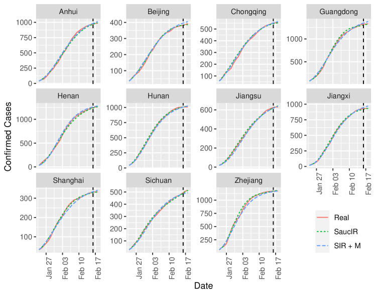
Figure 3: Predicted numbers of confirmed cases in selected provinces. The data on January 24 through February 15, 2020 were used to fit curves while the fitted models were used to forecast the confirmed case numbers on February 16-18, 2020.

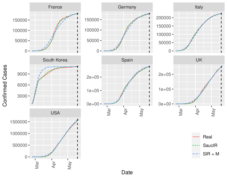
Figure 4: Predicted numbers of confirmed cases in selected countries. The data on February 24 through May 18, 2020 were used to fit curves while the fitted models were used to forecast the confirmed case numbers on May 19-21, 2020.

3.3 Impact of migration on confirmed cases

In this subsection, we study how the migration scales affect the confirmed cases. The epidemiological parameters and mobility parameters involved in the dynamic SaucIR model (2.8) are calculated or fitted based on the migration data obtained from the Baidu website and epidemic data announced officially from Janruary 24 to February 29, 2020.

The migration scale ($C_{nm,T}^{\textrm{in}}$ and $C_{nm,T}^{\textrm{out}}$) is categorized into three levels, where the large and medium scales are triple and twice of the small scale. Using optimal procedure (2.10), the coverage of confirmed cases can be obtained under various migration scales.

Table 15 summarizes the predicted confirmed cases on the nodes in the 11-province human mobility network of mainland China. Vertically, in the same scope of migration scale, the estimates confirmed cases do not vary much between the minimum and maximum. This implies that modifying the emanating rates from a node in or out of another node within the network has a minor impact on controlling the transmission rate. Horizontally, a smaller migration scale, less confirmed cases. This may be evidence of the validity of Wuhan lockdown for preventing the spread of COVID-19.

Table 15: Influence of migration scales on confirmed cases

	$C_{ij}$
Confirmed cases	Large	Medium	Small
Maximum	9481	9377	9268
Minimum	9439	9344	9251

4 Conclusion and Discussion

Compared to the SIR model raised in [Brockmann(2013)], our SaucIR model is disease specific for the spread of the COVID-19 pandemic. The primary difference is that the infection compartment has an independent segment of asymptomatic infected individuals based on the epidemiological characteristics of COVID-19. The numerical results indicate that such re-compartment is critical and substantial. By the time our revised manuscript was submitted, we found more studies on asymptomatic with considerable proportions up to 58% among patients with infection, justifying the rationale of independent A segment in the proposed compartmental model. The rate of asymptomatic per sons in population-based retrospective studies can even reach 43% [Gudbjartsson(2020)]. It remains a series of unsolved problems regarding the asymptomatic patients in COVID-19 that are anticipating more epidemiological observations and experiments, such as pattern of infectiveness, accurate communicable period, effective surveillance and screening [Lee(2020)]. The next distinction is that we present a dynamic migration procedure rather than fixing the mobility parameters. Baidu migration data source makes it feasible for modeling and computing. The advantage of such dynamic human mobility makes it possible to take into consideration of infection during the procedures of migration in and out of a spatial node, achieving the predictive fidelity of the proposed SaucIR model. On the other hand, it validates the necessity of the separation of moving in and out of the same node from other nodes in the modeling. The minor difference is that we use the absolute flux of population rather than the fraction of the passenger flux. The big population size of the provinces in China brings out a fraction of each compartment far less than unity, which has impact on the prediction accuracy. We need to point out that our modeling uses newly published parameters such as incubation days of infected to the symptom and asymptomatic to recovered. Modeling the spread pattern is an important issue and could be updated when there are new and reliable epidemic parameters.

The COVID-19 pandemic has not ended yet. The forecasting SaucIR model will benefit the public health authorities to assess the epidemic situation, make reasonably informed decisions, take appropriate interventions, and give a timely control of infection.

References

- [Kermack(1927)] Kermack W. O., McKendrick A. G., Walker G. T., 1927. A contribution to the mathematical theory of epidemics. Proceedings of the Royal Society of London. Series A: Mathematical and Physical Sciences. 115, 700–721.
- [Brockmann(2013)] Brockmann D., Helbing D., 2013. The Hidden Geometry of Complex, Network-Driven Contagion Phenomena. Science. 342, 1337–1342.
- [Pan(2020)] Pan A., Liu L., Wang C., Guo H., Hao X., Wang Q., Huang J., He N., Yu H., Lin X., Wei S., Wu T., 2020. Association of public health interventions with the epidemiology of the COVID-19 outbreak in Wuhan, China. The Journal of the American Medical Association. 323, 1915–1923.
- [Jia(2011)] Jia J. S., Lu X., Yuan Y. et al., (2020) Population flow drives spatio-temporal distribution of COVID-19 in China. Nature. 582, 389–394.
- [Petropoulos(2020)] Petropoulos F., Makridakis S., (2020) Forecasting the novel coronavirus COVID-19. PLoS ONE. 15, e0231236.
- [Gandhi(2020)] Gandhi M., Yokoe D. S., Havlir D. V., (2020) Asymptomatic transmission, the Achilles’ heel of current strategies to control COVID-19. New England Journal of Medicine. 382, 2158–2160.
- [Toda(2020)] Toda A. A., (2020) Susceptible-infected-recovered (SIR) dynamics of COVID-19 and economic impact. arXiv:2003.11221.
- [To(2020)] To K. K., Tsang O. T., Leung W. S. et al (2020) Temporal profiles of viral load in posterior oropharyngeal saliva samples and serum antibody responses during infection by SARS-CoV-2: An observational cohort study. The Lancet Infectious Diseases. 20, 565–574.
- [Hufnagel(2004)] Hufnagel L., Brockmann D., Geisel T. (2004) Forecast and control of epidemics in a globalized world. Proceedings of the National Academy of Sciences. 101, 15124–15129.
- [Chen(2020)] Chen B., Shi M., Ni X. et al. (2020) Data visualization analysis and simulation prediction for COVID-19. arXiv:2002.07096
- [Lauer(2020)] Lauer S. A., Grantz K. H., Bi Q. et al. (2020) The incubation period of coronavirus disease 2019 (COVID-19) from publicly reported confirmed cases: Estimation and application. Annals of Internal Medicine. 172, 577–582.
- [Rvachev(1985)] Rvachev L. A., Longini Jr I. M. (1985) A mathematical model for the global spread of influenza. Mathematical Biosciences. 75, 3–22.
- [Deb(1999)] Deb K. (1999) An Introduction to Genetic Algorithms. Sadhana. 24, 293–315.
- [Hu(2020)] Hu Z., Song C., Xu C., Jin G. et al. (2020) Clinical characteristics of 24 asymptomatic infections with COVID-19 screened among close contacts in Nanjing, China. Science China Life Sciences. 63, 1–6.
- [Mizumoto(2020)] Mizumoto K., Kagaya K., Zarebski A., Chowell G. (2020) Estimating the asymptomatic proportion of coronavirus disease 2019 (COVID-19) cases on board the Diamond Princess cruise ship, Yokohama, Japan, 2020. Eurosurveillance. 25, 2000180.
- [Nishiura(2020)] Nishiura H., Kobayashi T., Miyama T. et al. (2020) Estimation of the asymptomatic ratio of novel coronavirus infections (COVID-19). International Journal of Infectious Diseases. 94, 154–155.
- [Chowell(2003)] Chowell G., Fenimore P. W., Castillo-Garsow M. A., Castillo-Chavez C. (2003) SARS outbreaks in Ontario, Hong Kong and Singapore: The role of diagnosis and isolation as a control mechanism. Journal of Theoretical Biology. 224, 1–8.
- [Verity(2020)] Verity R., Okell L. C., Dorigatti I. et al. (2020) Estimates of the severity of coronavirus disease 2019: A model-based analysis. The Lancet Infectious Diseases. 20, 669–677.
- [Hao(2020)] Hao X., Cheng S., Wu D. et al. (2020) Reconstruction of the full transmission dynamics of COVID-19 in Wuhan. Nature. doi: 10.1038/s41586-020-2554-8.
- [Biotechnology(2020)] (2020) The COVID-19 testing debacle. Nature Biotechnology. 38, 653.
- [Bai(2020)] Bai Y., Yao L., Wei T. et al. (2020) Presumed asymptomatic carrier transmission of COVID-19. The Journal of the American Medical Association. 323, 1406–1407.
- [Callaway(2020)] Callaway E., Cyranoski D., Mallapaty S. et al. (2020) Coronavirus by the numbers. Nature. 579, 482–483.
- [Bertozzi(2020)] Bertozzi A. L., Franco E., Mohler G. et al. (2020) The challenges of modeling and forecasting the spread of COVID-19. Proceedings of the National Academy of Sciences. 117, 16732–16738.
- [Lee(2020)] Lee S., Kim T., Lee E. et al. (2020) Clinical course and molecular viral shedding among asymptomatic and symptomatic patients with SARS-CoV-2 infection in a community treatment center in the Republic of Korea. JAMA Internal Medicine. doi: 10.1001/jamainternmed.2020.3862.
- [Liu(2020)] Liu Y., Gayle A. A., Wilder-Smith A., Rocklöv J. (2020) The reproductive number of COVID-19 is higher compared to SARS coronavirus. Journal of Travel Medicine. 27
- [Li(2020)] Li P., Fu J. B., Lia K. F. et al (2020) Transmission of COVID-19 in the terminal stages of the incubation period: A familial cluster. International Journal of Infectious Diseases. 96, 452–453.
- [Gudbjartsson(2020)] Gudbjartsson D. F., Helgason A., Jonsson, H. (2020) Spread of SARS-CoV-2 in the Icelandic population. New England Journal of Medicine. 382, 2302-2315.
- [Infection] https://epidemic-stats.com/coronavirus/
- [Mainland-China-Infection] https://news.163.com/special/epidemic/
- [Migration] https://qianxi.baidu.com/2020/
- [Shanghai-Infection-Data] http://wsjkw.sh.gov.cn/xwfb/20200131/936f134cb3284c1db62d39c87ce5c501.html
- [Worldwide-Infection-Data] https://www.who.int/docs/default-source/coronaviruse/situation-reports/20200415-sitrep-86-covid-19.pdf?sfvrsn=c615ea20_6
- [Migration] www.oag.com