Floquet Second Order Topological Superconductor based on Unconventional Pairing

Abstract

We theoretically investigate the Floquet generation of second-order topological superconducting (SOTSC) phase in the high-temperature platform both in two-dimension (2D) and three-dimension (3D). Starting from a $d$-wave superconducting pairing gap, we periodically kick the mass term to engineer the dynamical SOTSC phase within a specific range of the strength of the drive. Under such dynamical breaking of time-reversal symmetry (TRS), we show the emergence of the weak SOTSC phase, harboring eight corner modes i.e.,  two zero-energy Majorana per corner, with vanishing Floquet quadrupole moment. On the other hand, our study interestingly indicates that upon the introduction of an explicit TRS breaking Zeeman field, the weak SOTSC phase can be transformed into strong SOTSC phase, hosting one zero-energy Majorana mode per corner, with quantized quadrupole moment. We also compute the Floquet Wannier spectra that further establishes the weak and strong nature of these phases. We numerically verify our protocol computing the exact Floquet operator in open boundary condition and then analytically validate our findings with the low energy effective theory (in the high-frequency limit). The above protocol is applicable for 3D as well where we find one dimensional (1D) hinge mode in the SOTSC phase. We then show that these corner modes are robust against moderate disorder and the topological invariants continue to exhibit quantized nature until disorder becomes substantially strong. The existence of zero-energy Majorana modes in these higher-order phases is guaranteed by the anti-unitary spectral symmetry.

I Introduction

The advent of topological superconductors (TSCs), harboring Majorana zero modes (MZMs) at their boundary, have generated immense interest in the quantum condensed matter community from both theoretical and experimental perspectives in the last few years Kitaev (2001); Qi and Zhang (2011); Hasan and Kane (2010); Das et al. (2012); Deng et al. (2016). Due to the non-Abelian statistics of the MZMs, they are proposed to be suitable candidates for the topological quantum computation Ivanov (2001); Nayak et al. (2008). There have been multitudinous proposals based on heterostructure setup of materials with strong spin-orbit coupling such as topological insulator, semiconductor thin films, and nanowires with the proximity induced superconductivity and Zeeman field, that provide an efficient platform to realize the MZMs Fu and Kane (2008); Sau et al. (2010); Lutchyn et al. (2010); Qi et al. (2010); Oreg et al. (2010).

In recent times, the concept of conventional bulk-boundary correspondence of topological phases in various topological systems such as topological insulators (TIs), Dirac semimetals (DSMs), Weyl semimetals (WSMs), TSCs, etc. have been generalized to higher-order topological (HOT) phases Benalcazar et al. (2017a, b); Song et al. (2017); Langbehn et al. (2017); Schindler et al. (2018); Khalaf (2018); Geier et al. (2018); Franca et al. (2018); Zhu (2018); Liu et al. (2018); Yan et al. (2018); Wang et al. (2019, 2018); Ezawa (2018); Călugăru et al. (2019); Trifunovic and Brouwer (2019); Zeng et al. (2019); Zhang et al. (2019a); Volpez et al. (2019); Yan (2019); Ghorashi et al. (2019, 2020); De et al. (2020); Wu et al. (2020); Laubscher et al. ; Roy (2020); Zhang and Trauzettel (2020); Zhang et al. (2020a, b); Kheirkhah et al. ; Plekhanov et al. . To be precise, an $n^{\rm th}$ order $d$-dimensional TI/ TSC exhibit gapless modes on their $(d-n)$-dimensional boundary ($n\leq d$). In particular, a 3D second (third) order TIs/TSCs are characterized by the presence of one (zero)-dimensional hinge (corner) modes, whereas, 2D second order topological insulators (SOTIs)/SOTSCs exhibit zero-dimensional (0D) corner modes only. There have been a few experimental proposals to realize 2D SOTIs hosting corner modes, based on acoustic materials Xue et al. (2019), photonic crystals Chen et al. (2019); Xie et al. (2019), and electrical circuit Imhof et al. (2018) setups.

Given the growing interest of the research community in this field, the non-equilibrium Floquet engineering emerges as a fertile hunch to generate the dynamical analog of the HOT phases. It has been shown that a trivial phase can be made topologically non-trivial with suitable periodic driving Lindner et al. (2011); Dóra et al. (2012); Rudner et al. (2013); Thakurathi et al. (2013); Rechtsman et al. (2013); Maczewsky et al. (2017); Eckardt (2017). The time translational symmetry of the problem causes the Floquet topological phase to host dissipationless dynamical topological boundary modes. The resulting bulk-boundary correspondence here becomes intriguing in the presence of the extra-temporal dimension. This non-equilibrium version of generating topological phase have been applied to HOTIs/HOTSCs resulting in Floquet HOTIs (FHOTIs) Bomantara et al. (2019); Nag et al. (2019); Peng and Refael (2019); Seshadri et al. (2019); Chaudhary et al. ; Rodriguez-Vega et al. (2019); Plekhanov et al. (2019); Ghosh et al. (2020); Huang and Liu (2020); Hu et al. (2020); Bomantara and Gong (2020); Peng (2020); Nag et al. ; Tiwari et al. ; Zhang and Yang ; Ghosh et al. ; Bhat and Bera ; Zhu et al. . However, the search for Floquet HOTSCs (FHOTSCs) is still at its initial stage Chaudhary et al. ; Plekhanov et al. (2019); Zhang et al. (2019b); Ghosh et al. ; Bomantara (2020) even from theoretical point of view.

In a very recent work, we show that the Floquet SOTSC phase can be engineered by kicking the time-reversal symmetry (TRS) breaking perturbation while the underlying static, $s$-wave proximitized parent system is in a trivial phase Ghosh et al. . In this article, we aim to generate Floquet SOTSC phase, hosting MZMs at the corner (hinges) for a 2D (3D) system, by suitably tuning some other parameter of the underlying first order TI such as the on-site mass term. Given the recent experimental advancements in Floquet systems based on solid state systems Wang et al. (2013a), meta-materials Rechtsman et al. (2013); Peng et al. (2016); Lejman et al. (2014); Fleury et al. (2016); Maczewsky et al. (2017), we believe that our question regarding the Floquet generation of MZMs in HOTSC phase is timely and pertinent. More importantly, the kicking of on-site term has been able to demonstrate a variety of interesting theoretical observation such as, Floquet topological insulator and superconductor Thakurathi et al. (2013); Seshadri et al. (2019); Čadež et al. (2019); Nag and Roy dynamical localization Nag et al. (2014); Agarwala et al. (2016), survival probability of initial state Patel, Aavishkar A. et al. (2013); Rajak and Dutta (2014) and thus motivates us to consider the on-site mass kicking dynamical protocol in order to obtain the desired outcome. However, the dynamical manipulation of mass term is yet to be experimentally realized. Moreover, the 2D TIs have been experimentally realized at high-temperature $100$ K Wu et al. (2018); Qian et al. (2014), paving the way to explore the high-temperature platform of MZMs.

To investigate the above mentioned possibility, we begin with a 2D TI in close proximity to a $d$-wave superconductor with unconventional pairing. Here, we consider the external drive to be periodically kicking the onsite mass term of the first order TI. This results in a weak Floquet SOTSC (FSOTSC) phase where two MZMs are localized at each corner of the 2D sample. Here the TRS is dynamically broken in the effective Floquet Hamiltonian. Remarkably, this degeneracy of two Majorana corner modes (MCMs) per corner can be lifted by incorporating an explicit TRS broken Zeeman field leading to a strong FSOTSC phase with one MZM per corner. We numerically study the exact Floquet operator to obtain the above mentioned results that are further verified by the low energy effective theory in the high-frequency approximation. We characterize the topological nature of these phases by the appropriate topological invariants as Floquet quadrupole moment (FQM) and Floquet Wannier spectra (FWS). We then extend our proposal to 3D where also we find the weak (strong) FSOTSC phase in absence (presence) of a homogeneous Zeeman field. Here, the corrresponding HOT phase hosts 1D Majorana hinge modes (MHMs). Furthermore, we investigate the effect of disorder on these Majorana corner modes (MCMs) and we find that these modes are robust against moderate disorder strength. The existence of the MZMs are protected by anti-unitary spectral symmetry in all of the above cases.

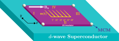
Figure 1: (Color online) Schematic of our setup is demonstrated in presence of a periodic kick (yellow, light grey) in the mass term as an external drive. Here, a 2D TI (violet, dark grey) is placed in close proximity to a bulk high-temperature $d$-wave superconductor (cyan, light grey). MCMs are shown by circular dots (grey) at the four corners of the 2D sample and the four edges of the TI are denoted by I, II, III, IV.

The remainder of the paper is organized as follows. In Sec. II, we introduce our model and the driving protocol. We illustrate the emergence of Floquet MCMs in the local density of states (LDOS) behavior. We resort to low energy edge theory to understand the emergence of the corner mode solutions. First, we solve these edge Hamiltonian to derive the corner mode solution. We characterize the MCMs using FQM and FWS. In Sec. III, we provide a protocol to generate 3D FSOTSC. We show the appearance of MHMs in rod geometry. We use low energy surface theory to confirm the existence of these hinge modes. Then we provide the analytical solutions for the hinge modes by solving the surface Hamiltonian. In Sec. IV, we study the effect of disorder on MZMs and show that they are robust against a finite amount of disorder. Finally in Sec. V, we summarize and conclude our results.

II Majorana Corner modes in 2D

In this section, we discuss in detail the model Hamiltonian of our set-up along with the driving protocol, the emergence of Floquet MCMs by numerically computing the exact Floquet evolution operator, low energy effective edge theory in the high-frequency regime and analytical understanding of the MCMs solutions therein.

II.1 Model Hamiltonian and Driving Protocol

II.1.1 Model

We consider the model of a 2D TI proximitized with $d$-wave superconductivity on a square lattice Yan et al. (2018). The experimental realization of high-temperature 2D TI allows us to consider proximity induced high-temperature superconductor Wu et al. (2018); Qian et al. (2014). It acquires the following form while written in Bogoliubov-de Gennes (BdG) basis $H_{\rm BdG}=\frac{1}{2}\sum_{{\bm{\mathrm{k}}}}\Psi^{\dagger}_{\bm{\mathrm{k}}}\mathcal{H}_{0}({\bm{\mathrm{k}}})\Psi_{\bm{\mathrm{k}}}$, with $\Psi_{\bm{\mathrm{k}}}=\left(c_{{\bm{\mathrm{k}}},a\uparrow},c_{-{\bm{\mathrm{k}}},a\uparrow}^{\dagger},c_{{\bm{\mathrm{k}}},a\downarrow},c_{-{\bm{\mathrm{k}}},a\downarrow}^{\dagger},c_{{\bm{\mathrm{k}}},b\uparrow},c_{-{\bm{\mathrm{k}}},b\uparrow}^{\dagger},c_{{\bm{\mathrm{k}}},b\downarrow},c_{-{\bm{\mathrm{k}}},b\downarrow}^{\dagger}\right)^{\tilde{T}}$ and $\mathcal{H}_{0}({\bm{\mathrm{k}}})$, is given by

$$\mathcal{H}_{0}({\bm{\mathrm{k}}}) = \epsilon(\bm{\mathrm{k}})\Gamma_{1}+\lambda_{x}\sin k_{x}\Gamma_{2}+\lambda_{y}\sin k_{y}\Gamma_{3}+\Delta(\bm{\mathrm{k}})\Gamma_{4}$$ (1)

$$+B_{x}\Gamma_{5}\equiv{\bm{\mathrm{N}}}(\bm{\mathrm{k}})\cdot{\bm{\Gamma}}\ ,$$

Here, $t_{x,y}$ and $\lambda_{x,y}$ represent the nearest-neighbour hopping and spin-orbit coupling respectively, $\epsilon(\bm{\mathrm{k}})=\left(m_{0}-t_{x}\cos k_{x}-t_{y}\cos k_{y}\right)$, $\Delta(\bm{\mathrm{k}})=\Delta_{0}\left(\cos k_{x}-\cos k_{y}\right)$ is the $d$-wave superconducting paring term, $m_{0}$ is the crystal-field splitting energy. In Eq.(1), $\Gamma_{1}=\sigma_{z}\tau_{z}$, $\Gamma_{2}=\sigma_{x}s_{z}$, $\Gamma_{3}=\sigma_{y}\tau_{z}$, $\Gamma_{4}=s_{y}\tau_{y}$ and $\Gamma_{5}=s_{x}\tau_{z}$. The three Pauli matrices ${\bm{\sigma}}$, ${\bm{s}}$ and ${\bm{\tau}}$ act on orbital $(a,b)$, spin $(\uparrow,\downarrow)$ and particle-hole degrees of freedom respectively. When $B_{x}=0$, the system respects TRS i.e.,  $\mathcal{T}^{-1}\mathcal{H}_{0}(\bm{\mathrm{k}})\mathcal{T}=\mathcal{H}_{0}(-\bm{\mathrm{k}})$ with $\mathcal{T}=is_{y}\mathcal{K}$, $\mathcal{K}$ being the complex-conjugation operator. The Hamiltonian continues to preserve the particle-hole symmetry (PHS) $\mathcal{C}^{-1}\mathcal{H}_{0}(\bm{\mathrm{k}})\mathcal{C}=-\mathcal{H}_{0}(-\bm{\mathrm{k}})$ with $\mathcal{C}=\tau_{x}\mathcal{K}$ for $B_{x}\neq 0$. Below we discuss the properties of our model at length.

First, we discuss the topological nature associated with the Hamiltonian (Eq.(1)) for $\Delta(\bm{\mathrm{k}})=0$ and $B_{x}=0$. This model supports topological phase, hosting gapless helical edge modes, when $|m_{0}|<t_{x}+t_{y}$. For $|m_{0}|>t_{x}+t_{y}$, the model becomes trivially gapped. Upon the introduction of $d$-wave pairing only i.e.,  $\Delta(\bm{\mathrm{k}})\neq 0$ and $B_{x}=0$, the 1D massless Dirac fermions representing the edge modes of TI phase, become gapped by the induced unconventional superconducting pairing. However, the specific nature of pairing symmetry causes the Dirac mass to change signs at the corners. This in turn generates MCMs, a signature of SOTSC phase for TRS invariant TSC system, as domain-wall excitations when $|m_{0}|<t_{x}+t_{y}$. Here, one can observe Majorana Kramers pair (MKPs) (i.e.,  two Majoranas per corner are time-reversal partners of each other) pinned at zero-energy which are protected by the TRS. When $|m_{0}|>t_{x}+t_{y}$, the underlying TI becomes non-topological and $d$-wave pairing cannot lead to MKPs anymore as the system becomes gapped. Now, in presence of TRS breaking Zeeman field $B_{x}\neq 0$, the degeneracy of MKPs can be lifted by destroying one mode in the pair at the corner. Therefore, the Hamiltonian supports MZMs with one Majorana per corner for $\Delta(\bm{\mathrm{k}})\neq 0$ and $B_{x}\neq 0$ while $|m_{0}|<t_{x}+t_{y}$. The magnetic field allows us to tune the bulk gap which is introduced by the superconducting order parameter $\Delta(\bm{\mathrm{k}})$. Given this background, it would be interesting to study the emergence of MCMs starting from the underlying non-topological phase $|m_{0}|>t_{x}+t_{y}$ by periodically kicking the mass with a finite amplitude and frequency.

II.1.2 Driving Protocol and Floquet Operator

Here we introduce our driving protocol in the form of periodic kick in the mass term as discussed before

$$m(t) = m_{1}\sum_{r=1}^{\infty}\delta(t-rT)\ ,$$ (2)

with $r$ being an integer. This driving protocol allows one to write the exact Floquet operator in the following way using the time ordered (${\rm\bf TO}$) notation as

$$U(T) = {\rm\bf TO}\exp\left[-i\int_{0}^{T}dt\left(\mathcal{H}_{0}({\bm{\mathrm{k}}})+m(t)\Gamma_{1}\right)\right]$$ (3)

$$= \exp(-i\mathcal{H}_{0}({\bm{\mathrm{k}}})T)~{}\exp(-im_{1}\Gamma_{1})\ .$$

Here, $T$, $m_{1}$ are the period and amplitude of the drive respectively. The above decomposition essentially means that the system is freely evolved between two subsequent kicks. The Floquet operator $U(T)$ can be written in a more compact form as follows

$$U(T) = C_{T}\left(p-iq\Gamma_{1}\right)-iS_{T}\sum_{j=1}^{5}\left(n_{j}\Gamma_{j}+m_{j}\Gamma_{j1}\right)\ ,$$ (4)

where, $C_{T}=\cos(\left|{\bm{\mathrm{N}}}(\bm{\mathrm{k}})\right|T)$, $S_{T}=\sin(\left|{\bm{\mathrm{N}}}(\bm{\mathrm{k}})\right|T)$, $p=\cos m_{1}$, $q=\sin m_{1}$, $n_{j}=\frac{N_{j}(\bm{\mathrm{k}})\cos m_{1}}{\left|{\bm{\mathrm{N}}}(\bm{\mathrm{k}})\right|}$, $m_{j}=\frac{N_{j}(\bm{\mathrm{k}})\sin m_{1}}{\left|{\bm{\mathrm{N}}}(\bm{\mathrm{k}})\right|}$ and $\Gamma_{j1}=\frac{1}{2i}\left[\Gamma_{j},\Gamma_{1}\right]$ with $j=2,3,4,5$. One can thus obtain the general form of the effective Hamiltonian as

$$H_{\rm Flq}=\frac{\xi_{\bm{\mathrm{k}}}}{\sin\xi_{\bm{\mathrm{k}}}T}\Bigg{[}\sin(\left|{\bm{\mathrm{N}}}(\bm{\mathrm{k}})\right|T)\cos m_{1}\sum_{j=1}^{5}r_{j}\Gamma_{j}+\cos(\left|{\bm{\mathrm{N}}}(\bm{\mathrm{k}})\right|T)\sin m_{1}\Gamma_{1}+\sin(\left|{\bm{\mathrm{N}}}(\bm{\mathrm{k}})\right|T)\sin m_{1}\sum_{j=2}^{5}r_{j}\Gamma_{j1}\Bigg{]}\ ,$$ (5)

with $\xi_{\bm{\mathrm{k}}}=\frac{1}{T}\cos^{-1}\left[\cos(\left|{\bm{\mathrm{N}}}(\bm{\mathrm{k}})\right|T)\cos m_{1}\right]$, $r_{j}=\frac{N_{j}(\bm{\mathrm{k}})}{\left|{\bm{\mathrm{N}}}(\bm{\mathrm{k}})\right|}$. In the high-frequency limit i.e.,   $T\rightarrow 0$ and small amplitude of drive i.e.,   $m_{1}\rightarrow 0$, one can neglect the higher order terms in $T$ and $m_{1}$. Thus, the effective Hamiltonian in that limit reads as

$$H_{\rm Flq}\approx\mathcal{H}_{0}(\bm{\mathrm{k}})+\frac{m_{1}}{T}\Gamma_{1}+m_{1}\sum_{j=2}^{5}r_{j}\Gamma_{j1}\ .$$ (6)

In Eq.(6), terms associated with $\Gamma_{j1}$ are originated due to the driving and not present in the static Hamiltonian (Eq.(1)). It is noteworthy that these extra $r_{j}\Gamma_{j1}$ terms break TRS $\mathcal{T}$ in the system. Consequently, the above Hamiltonian breaks TRS $\mathcal{T}$ even when $B_{x}=0$. This reflects the fact that the TRS can be broken dynamically by mass kicking while the static perturbation respects the TRS. Therefore, it would be important to study the effect of these terms in the dynamics with and without the magnetic field. The former situation can be referred to as the explicit breaking of TRS while the later is related to the dynamical breaking of TRS. At the outset, we would like to comment from Eq.(6) that the mass term gets renormalized by the driving $m_{0}\to m_{0}+m_{1}/T$. Therefore, the topological phase boundary is thus got renormalized. Hence, MCMs can be found when $|m_{0}+m_{1}/T|<t_{x}+t_{y}$ with $\Delta(\bm{\mathrm{k}})\neq 0$ and $B_{x}\neq 0$. Similar to the static case, here also for the Floquet case the magnetic field allows us to tune the bulk gap which is introduced by the superconducting order parameter $\Delta(\bm{\mathrm{k}})$. This would lead to analytical handling which we describe below in terms of the low energy effective model. In the presence of $\Delta$, interestingly, we find $H_{\rm Flq}$ continues to preserve the anti-unitary PHS generated by $\mathcal{C}$. This anti-unitary symmetry is essential to localize the MCMs at zero-energy associated with the effective Hamiltonian (Eq.(6)). Here, we would like to emphasize that we make use of the High-frequency Hamiltonian (Eq.(6)) only to corroborate the existence of the dressed corner modes which we obtain from the exact diagonalization of the Floquet Operator $U(T)$ (Eq.(3)).

II.2 Floquet Corner mode

Having established the possible route to an analytical understanding of the emergence of MZMs, we here numerically show their existence in the 2D FSOTSC phase that is characterized by the presence of Floquet MCMs. To be precise, we find the signature of dynamical MCMs that appear in the Floquet LDOS as shown in Fig. 2. We know $U(T)|\phi_{m}\rangle=\exp(-i\mu_{m}T)|\phi_{m}\rangle$, where $|\phi_{m}\rangle$ is the Floquet quasi-energy states corresponding to the Floquet quasi-energy $\mu_{m}$. To calculate the LDOS, we numerically diagonalize the Floquet operator, $U(T)$ (in Eq.(3)) in the open boundary condition (OBC) . Here, we consider the Floquet eigenmodes $|\phi_{m}\rangle$’s associated with $\mu_{m}\approx 0$ (within numerical accuracy) to compute the LDOS of these zero-energy states. These MCMs can be easily distinguished from the gapped bulk modes. Note that, the 2D SOTSC phase hosting MCMs has been very recently studied in static  Wu et al. (2020); Volpez et al. (2019); Yan et al. (2018); Yan (2019) and Floquet driven Plekhanov et al. (2019); Ghosh et al. cases with different driving protocols.

We consider two cases, in the first case, we set the amplitude of the in-plane magnetic field, $B_{x}=0$, and the corresponding LDOS is shown in Fig. 2(a). One can identify from the inset of Fig. 2(a) that there exist eight MCMs i.e.,  two MZMs per corner. While for $B_{x}\neq 0$, we obtain four MCMs i.e.,  one MZM per corner as depicted in the inset of Fig. 2(b). One can thus infer from Fig. 2(a) that two MZMs sharing the same corner annihilate each other to give rise to an electronic corner mode which may lead to a weak FSOTSC phase. Interestingly, in Fig. 2(b) the applied in-plane magnetic field yields only one MZM per corner carrying a signature of strong FSOTSC phase Ghosh et al. . Moreover, the localization properties of these MCMs are significantly modified with the introduction of the Zeeman field. From the weight structure of MCMs as observed in LDOS, it is evident that the localization length remains the same in $x$ and $y$ direction for $B_{x}=0$. Finite $B_{x}$ breaks this symmetry of localization length and the weight becomes less along the $y$ direction as compared to the $x$ direction. The introduction of $B_{y}$ instead of $B_{x}$ does not change these properties. We discuss more regarding this in the later part of the paper.

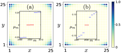
Figure 2: (Color online) (a) The behavior of LDOS, associated with the MCMs at $\mu_{m}=0$, is demonstrated for $B_{x}=0$ considering finite geometry. The inset exhibits the Floquet quasi-energy spectrum $\mu_{m}$ as a function of $m$ where eight MZMs are observed. Here, $L_{x}=L_{y}=25,t_{x}=t_{y}=\lambda_{x}=\lambda_{y}=1.0,m_{0}=2.5$, $\Delta=0.6,m_{1}=-0.4,T=0.419$. (b) LDOS in finite geometry and eigenvalue spectrum (inset) are depicted for $B_{x}=0.3$. Here four MZMs appear at quasi-energy $\mu_{m}=0$. The number of MCMs at $\mu_{m}=0$ can be reduced to half upon the introduction of the Zeeman field.

II.3 Low energy edge theory

Here, we turn ourself to the low energy edge theory to corroborate the findings of the MCMs. We begin by expanding the effective Hamiltonian in the high-frequency limit (Eq.(6)) around $\Gamma=(0,0)$ point as

$$H_{\rm Flq,\Gamma} \approx \left(m^{\prime}-\frac{t_{x}}{2}k_{x}^{2}-\frac{t_{y}}{2}k_{y}^{2}\right)\Gamma_{1}+\lambda_{x}k_{x}\Gamma_{2}+\lambda_{y}k_{y}\Gamma_{3}$$ (7)

$$-\frac{\Delta}{2}\left(k_{x}^{2}-k_{y}^{2}\right)\Gamma_{4}+B_{x}\Gamma_{5}+\frac{m_{1}}{T}\Gamma_{1}+m_{1}\lambda_{x}k_{x}\Gamma_{21}$$

$$+m_{1}\lambda_{y}k_{y}\Gamma_{31}-\frac{m_{1}\Delta}{2}\left(k_{x}^{2}-k_{y}^{2}\right)\Gamma_{41}\ ,$$

where, $m^{\prime}=\left(m_{0}-t_{x}-t_{y}\right)$, $\Gamma_{21}=-\sigma_{y}s_{z}\tau_{z}$, $\Gamma_{31}=\sigma_{x}$ and $\Gamma_{41}=\sigma_{z}s_{y}\tau_{x}$. For a demonstrative example, we present the analytical solution for edge-I. We consider here open (periodic) boundary condition along $x$ ($y$) direction. We rewrite $H_{\rm Flq,\Gamma}=H_{0}(-i\partial_{x})+H_{p}(-i\partial_{x},k_{y})$ by replacing $k_{x}\rightarrow-i\partial_{x}$ and neglecting $k_{y}^{2}$ term. We thus obtain

$$H_{0} = \left(m-\frac{t_{x}}{2}\partial_{x}^{2}\right)\Gamma_{1}-i\lambda_{x}\partial_{x}\ \Gamma_{2}\ ,$$

$$H_{p} = \lambda_{y}k_{y}\Gamma_{3}+\frac{\Delta}{2}\partial_{x}^{2}\ \Gamma_{4}+B_{x}\Gamma_{5}-im_{1}\lambda_{x}\partial_{x}\ \Gamma_{21}$$ (8)

$$+m_{1}\lambda_{y}k_{y}\Gamma_{31}+\frac{m_{1}\Delta}{2}\partial_{x}^{2}\ \Gamma_{41}\ .$$

Here, we consider the pairing amplitude $\Delta$ and the amplitude of the in-plane magnetic field $B_{x}$ to be small and treat them as small perturbation Yan et al. (2018); Yan (2019); Ghosh et al. . The mass term $m=\left(m^{\prime}+\frac{m_{1}}{T}\right)$ is considered to be less than zero. Assuming $\Psi$ to be the zero-energy eigenstate of $H_{0}$ and following the boundary condition $\Psi(x=0)=\Psi(x=\infty)=0$, we obtain

$$\Psi_{\alpha}=\left|\mathcal{N}_{x}\right|^{2}e^{-\mathcal{K}_{1}x}\sin\mathcal{K}_{2}x\ e^{ik_{y}y}\Phi_{\alpha}\ ,$$ (9)

where, $\mathcal{K}_{1}=\frac{\lambda_{x}}{t_{x}}$, $\mathcal{K}_{2}=\sqrt{\left|\frac{m}{t_{x}}\right|-\mathcal{K}_{1}^{2}}$, $\left|\mathcal{N}_{x}\right|^{2}=\frac{4\mathcal{K}_{1}\left(\mathcal{K}_{1}^{2}+\mathcal{K}_{2}^{2}\right)}{\mathcal{K}_{2}^{2}}$ and $\Phi_{\alpha}$ is a 8-component spinor satisfying $\sigma_{y}s_{z}\tau_{z}\Phi_{\alpha}=-\Phi_{\alpha}$. Our chosen basis reads

$$\Phi_{1} = \ket{\sigma_{y}=+1}\otimes\ket{s_{z}=+1}\otimes\ket{\tau_{z}=-1},$$

$$\Phi_{2} = \ket{\sigma_{y}=-1}\otimes\ket{s_{z}=+1}\otimes\ket{\tau_{z}=+1},$$

$$\Phi_{3} = \ket{\sigma_{y}=-1}\otimes\ket{s_{z}=-1}\otimes\ket{\tau_{z}=-1},$$

$$\Phi_{4} = \ket{\sigma_{y}=+1}\otimes\ket{s_{z}=-1}\otimes\ket{\tau_{z}=+1}\ .$$ (10)

The matrix element of $H_{p}$ in this basis can be written as

$$H_{\rm I,\alpha\beta}^{\rm Edge}=\int_{0}^{\infty}dx\ \Psi_{\alpha}^{\dagger}(x)H_{p}(-i\partial_{x},k_{y})\Psi_{\beta}(x)\ ,$$ (11)

Thus, we obtain the effective Hamiltonian for the edge-I as

$$H_{\rm I}^{\rm Edge}=-\lambda_{y}k_{y}s_{z}+M_{\rm I}s_{y}\tau_{y}\ ,$$ (12)

where, $M_{\rm I}=\lvert\frac{m\Delta}{t_{x}}\rvert$. Similarly, for edge-II, III and IV, one can obtain the effective Hamiltonian as

$$H_{\rm II}^{\rm Edge} = \lambda_{x}k_{x}s_{z}-M_{\rm II}s_{y}\tau_{y}-B_{x}s_{x}\tau_{z}\ ,$$

$$H_{\rm III}^{\rm Edge} = -\lambda_{y}k_{y}s_{z}+M_{\rm III}s_{y}\tau_{y}\ ,$$

$$H_{\rm IV}^{\rm Edge} = \lambda_{x}k_{x}s_{z}-M_{\rm IV}s_{y}\tau_{y}-B_{x}s_{x}\tau_{z}\ .$$ (13)

where, $M_{\rm II}=\lvert\frac{m\Delta}{t_{y}}\rvert$, $M_{\rm III}=M_{\rm I}$ and $M_{\rm IV}=M_{\rm II}$. Therefore, the low energy effective Hamiltonian written in the edge co-ordinate $j$ is given by the compact form as

$$H_{j}^{\rm Edge}=-i\lambda(j)s_{z}\partial_{j}+M(j)s_{y}\tau_{y}-B(j)s_{x}\tau_{z}\ ,$$ (14)

with $\lambda(j)=\left\{-\lambda_{y},\lambda_{x},-\lambda_{y},\lambda_{x}\right\}$, $M(j)=\left\{M_{\rm I},-M_{\rm II},M_{\rm III},-M_{\rm IV}\right\}$ and $B(j)=\left\{0,B_{x},0,B_{x}\right\}$. Note that, one can consider $B_{y}$ instead of $B_{x}$; however, the above results do not change qualitatively. Now to proceed further we study two cases.

II.3.1 Case I: $B_{x}=0$

First, we turn-off the in-plane magnetic field $B_{x}$. The edge Hamiltonian $H_{j}^{\rm Edge}$ can be decomposed into two independent blocks as

$$H^{\rm Edge}_{j}=H_{\tau_{y}=+1}\oplus H_{\tau_{y}=-1}\ ,$$ (15)

where,

$$H_{\tau_{y}=+1} = -i\lambda(j)s_{z}\partial_{j}+M(j)s_{y}\ ,$$

$$H_{\tau_{y}=-1} = -i\lambda(j)s_{z}\partial_{j}-M(j)s_{y}\ .$$ (16)

We obtain domain walls for both these blocks $\tau_{y}=\pm 1$ as the mass term $M(j)$ changes its sign between two adjacent edges; from edge-I, III to edge-II, IV. In terms of the system parameters the Dirac mass changes from $\lvert\frac{m\Delta}{t_{x}}\rvert$ to $-\lvert\frac{m\Delta}{t_{y}}\rvert$. Consequently, one finds two MZMs per corner (see Fig. 2(a)); each block is giving rise to one MZM per corner. Therefore, one finds the origin of MCMs at each corner as obtained from the above low-energy edge theory. The dynamical breaking of TRS is only thus able to generate weak FSOTSC phase (see text for discussion).

II.3.2 Case II: $B_{x}\neq 0$

Incorporating the Zeeman field $B_{x}\neq 0$, in $\tau_{x}=s_{z}$ subspace, the last term in Eq.(14) can be written as $B(j)s_{x}\tau_{z}\rightarrow\mp B(j)s_{y}$ for $\tau_{y}=\pm 1$ block. The edge Hamiltonian $H_{j}^{\rm Edge}=H_{\tau_{y}=+1}\oplus H_{\tau_{y}=-1}$ thus takes the following form upon decomposing into two independent blocks as

$$H_{\tau_{y}=+1} = -i\lambda(j)s_{z}\partial_{j}+D(j)s_{y}\ ,$$

$$H_{\tau_{y}=-1} = -i\lambda(j)s_{z}\partial_{j}-D^{\prime}(j)s_{y}\ ,$$ (17)

with $D(j)=\{D_{\rm I},D_{\rm II},D_{\rm III},D_{\rm IV}\}=M(j)+B(j)$ and $D^{\prime}(j)=\{D^{\prime}_{\rm I},D^{\prime}_{\rm II},D^{\prime}_{\rm III},D^{\prime}_{\rm IV}\}=M(j)-B(j)$. Hence, one can eventually obtain two decoupled diagonal blocks with Dirac masses in different edges as $D_{\rm I}=\lvert\frac{m\Delta}{t_{x}}\rvert$, $D_{\rm II}=-\lvert\frac{m\Delta}{t_{y}}\rvert+B_{x}$, $D_{\rm III}=\lvert\frac{m\Delta}{t_{x}}\rvert$ and $D_{\rm IV}=-\lvert\frac{m\Delta}{t_{y}}\rvert+B_{x}$; $D^{\prime}_{\rm I}=D_{I}$, $D^{\prime}_{\rm II}=-\lvert\frac{m\Delta}{t_{y}}\rvert-B_{x}$, $D^{\prime}_{\rm III}=D_{III}$ and $D^{\prime}_{\rm IV}=-\lvert\frac{m\Delta}{t_{y}}\rvert-B_{x}$. Therefore, we observe that $B_{x}$ can change the gap along edge-II and IV leaving edge-I and III unaltered for both of these blocks. It is now quite evident from Eq.(17) that $B_{x}=\lvert\frac{m\Delta}{t_{y}}\rvert$ ($B_{x}=-\lvert\frac{m\Delta}{t_{y}}\rvert$) refers to a special situation where edge-II and IV become gapless for $\tau_{y}=+1$ ($\tau_{y}=-1$) block. This is in sharp contrast to the edge Hamiltonian without magnetic field as described in Eq.(16) where all the four edges are massive. In the present case with magnetic field $B_{x}=\lvert\frac{m\Delta}{t_{y}}\rvert$ ($B_{x}=-\lvert\frac{m\Delta}{t_{y}}\rvert$), the remaining two edges become massive for $\tau_{y}=+1$ ($\tau_{y}=-1$) block. We consider only positive values of $B_{x}$ and due to that reason we investigate two instances where $B_{x}>\lvert\frac{m\Delta}{t_{y}}\rvert$ and $B_{x}<\lvert\frac{m\Delta}{t_{y}}\rvert$.

When we consider $B_{x}>\lvert\frac{m\Delta}{t_{y}}\rvert$, $D^{\prime}(j)$ changes its sign from edge-I (III) to edge-II (IV) while $D(j)$ remains positive in all the four edges. Therefore, $\tau_{y}=+1$ block becomes inactive and remains always massive while $\tau_{y}=-1$, being the only active block, can lead to Jackie-Rebbi localized MCMs at zero quasi-energy. One can thus observe one MZM per corner as depicted in Fig. 2(b). On the other hand, for $B_{x}<\lvert\frac{m\Delta}{t_{y}}\rvert$, both the blocks turn out to be active i.e., mass changes its sign between two adjacent edges. Hence the MZMs are supported by both of these blocks. This would result in two MZMs per corner similar to the LDOS as shown in Fig. 2(a). Therefore, the explicit breaking of TRS by applying the magnetic field appears to be more efficient to obtain the FSOTSC phase as both weak (two MZM per corner) and strong (one MZM per corner) phases can be explored simultaneously. By contrast, the dynamical breaking of TRS without applying the magnetic field only allows us to explore the weak FSOTSC phase. We explain these phases more elaborately while discussing the topological invariants.

II.4 Corner Mode solution

II.4.1 Case I: $B_{x}=0$

To obtain the analytical solution of the MCMs, residing at the intersection between edge-I and II, we solve the corresponding edge Hamiltonians for the zero-energy solution. At edge-I, we assume a solution of the form

$$\Psi_{C}\sim e^{-\xi y}\left(a_{1},a_{2},a_{3},a_{4}\right)^{\tilde{T}}\ ,$$ (18)

Here, $\tilde{T}$ denotes the transpose. The eigenvalue equation for $\Psi_{C}$ acquires the following form

$$\begin{pmatrix}-i\lambda_{y}\xi&0&0&-M_{\rm I}\\ 0&-i\lambda_{y}\xi&M_{\rm I}&0\\ 0&M_{\rm I}&i\lambda_{y}\xi&0\\ -M_{\rm I}&0&0&i\lambda_{y}\xi\end{pmatrix}\begin{pmatrix}a_{1}\\ a_{2}\\ a_{3}\\ a_{4}\end{pmatrix}=0.$$ (19)

The secular equation for $\Psi_{C}$ then reads

$$\det\begin{pmatrix}-i\lambda_{y}\xi&0&0&-M_{\rm I}\\ 0&-i\lambda_{y}\xi&M_{\rm I}&0\\ 0&M_{\rm I}&i\lambda_{y}\xi&0\\ -M_{\rm I}&0&0&i\lambda_{y}\xi\end{pmatrix}=0\ .$$ (20)

Solving Eq.(20), we find four solutions for $\xi$ as

$$\xi=\left\{-\frac{M_{\rm I}}{\lambda_{y}},-\frac{M_{\rm I}}{\lambda_{y}},\frac{M_{\rm I}}{\lambda_{y}},\frac{M_{\rm I}}{\lambda_{y}}\right\}\ .$$ (21)

Given the fact that $\Psi_{C}$ must vanish at $y\rightarrow\infty$, therefore, we obtain two linearly independent solutions for edge-I, $\Phi_{C}^{\rm I,1}=(1,1,i,-i)^{\tilde{T}}$ and $\Phi_{C}^{\rm I,2}=(1,-1,-i,-i)^{\tilde{T}}$. Thus, $\Psi_{C}$ can be expanded as

$$\Psi_{C}\sim\alpha_{\rm I}\ e^{-\frac{M_{\rm I}}{\lambda_{y}}y}\Phi^{\rm I,1}_{C}\ +\ \beta_{\rm I}\ e^{-\frac{M_{\rm I}}{\lambda_{y}}y}\Phi^{\rm I,2}_{C}\ ,$$ (22)

Here, $\alpha_{\rm I}$ and $\beta_{\rm I}$ are the normalization factors for edge-I. Similarly, for edge-II with $\alpha_{\rm II}$ and $\beta_{\rm II}$ being the normalization factors, we obtain

$$\Psi_{C}\sim\alpha_{\rm II}\ e^{-\frac{M_{\rm II}}{\lambda_{x}}x}\Phi^{\rm II,1}_{C}\ +\ \beta_{\rm II}\ e^{-\frac{M_{\rm II}}{\lambda_{x}}x}\Phi^{\rm II,2}_{C}\ ,$$ (23)

where, $\Phi_{C}^{\rm II,1}=(1,1,i,-i)^{\tilde{T}}$ and $\Phi_{C}^{\rm II,2}=(1,-1,-i,-i)^{\tilde{T}}$. Considering the wavefuction, $\Psi_{C}$ to be continuous at the interface i.e.,  at $x=y=0$, we obtain $\alpha_{\rm I}=\alpha_{\rm II}=\alpha$ and $\beta_{\rm I}=\beta_{\rm II}=\beta$. Hence, the wavefunction for the MCMs becomes

$$\Psi_{C} \sim \alpha\ e^{-\frac{M_{\rm I}}{\lambda_{y}}y}\Phi^{\rm I,1}_{C}\ +\ \beta\ e^{-\frac{M_{\rm I}}{\lambda_{y}}y}\Phi^{\rm I,2}_{C}\ \quad\ {\rm:edge-I}\ ,$$

$$\Psi_{C} \sim \alpha\ e^{-\frac{M_{\rm II}}{\lambda_{x}}x}\Phi^{\rm I,1}_{C}\ +\ \beta\ e^{-\frac{M_{\rm II}}{\lambda_{x}}x}\Phi^{\rm I,2}_{C}\ \quad{\rm:edge-II}\ .$$

The localization length in the $x$ ($y$)-direction becomes $\lambda_{x}/M_{\rm II}$ ($\lambda_{y}/M_{\rm I}$). This clearly suggests that localization lengths of MCMs are dependent on the strength of hopping, spin-orbit coupling, mass, proximity induced superconducting gap function. In the present case, choice of $t_{x}=t_{y}$ and $\lambda_{x}=\lambda_{y}$ leads to the fact the localization length becomes uniform in $x$ and $y$-direction as observed in the Floquet LDOS (see Fig. 2(a)). More importantly, one can observe that there exist two MZMs at each corner corroborating our numerical findings as shown in the inset of Fig. 2(a). The presence of two MCMs suggests that they would annihilate each other leaving an electronic state at the corner. The dynamical breaking of TRS thus leads to a weak FSOTSC phase as each corner is occupied by two MCMs.

II.4.2 Case II: $B_{x}\neq 0$

Here we investigate the solutions for the MCMs in presence of $B_{x}$. To begin with, we assume $B_{x}>M_{\rm II}$. We proceed as before and obtain the following solutions for edge-I and II as

$$\Psi_{C} \sim \alpha_{\rm I}\ e^{-\frac{M_{\rm I}}{\lambda_{y}}y}\Phi^{\rm I,1}_{C}\ +\ \beta_{\rm I}\ e^{-\frac{M_{\rm I}}{\lambda_{y}}y}\Phi^{\rm I,2}_{C}\ \qquad\qquad\quad\ {\rm:edge-I},$$

$$\Psi_{C} \sim \alpha_{\rm II}\ e^{-\frac{B_{x}-M_{\rm II}}{\lambda_{x}}x}\Phi^{\rm II,1}_{C}\ +\ \beta_{\rm II}\ e^{-\frac{B_{x}+M_{\rm II}}{\lambda_{x}}x}\Phi^{\rm II,2}_{C}\ \ {\rm:edge-II},$$

where, $\Phi_{C}^{\rm I,1}=(1,1,i,-i)^{\tilde{T}}$, $\Phi_{C}^{\rm I,2}=(1,-1,-i,-i)^{\tilde{T}}$, $\Phi_{C}^{\rm II,1}=(1,-1,i,i)^{\tilde{T}}$ and $\Phi_{C}^{\rm II,2}=(1,1,i,-i)^{\tilde{T}}$. Upon matching $\Psi_{C}$ at the boundary, we obtain $\alpha_{\rm I}=\beta_{\rm II}=\alpha$ and $\beta_{\rm I}=\alpha_{\rm II}=0$. The final solution becomes

$$\Psi_{C} \sim \alpha~{}e^{-\frac{M_{\rm I}}{\lambda_{y}}y}\Phi^{\rm I,1}_{C}\qquad\qquad\ {\rm:edge-I},$$

$$\Psi_{C} \sim \alpha~{}e^{-\frac{B_{x}+M_{\rm II}}{\lambda_{x}}x}\Phi^{\rm I,1}_{C}\ \qquad\ {\rm:edge-II}.$$

In this case, the localization lengths are given by $\lambda_{x}/(B_{x}+M_{\rm II})$ ($\lambda_{y}/M_{\rm I}$) along $x$ ($y$)-direction. Thus the MCMs decay differently along the two directions into the bulk. This is also evident from the Floquet LDOS where localization of MZMs at the corners are stronger in $y$-direction as compared to $x$-direction (see Fig. 2(b)). Moreover, there exists one MCM per corner, as shown in the inset of Fig. 2(b). The presence of one MCMs suggests that it corresponds to a strong FSOTSC phase when $B_{x}\neq 0$. This phase cannot be realized in presence of only periodic kick drive i.e.,  when TRS is broken dynamically.

Furthermore, when $B_{x}<M_{\rm II}$, we continue to obtain two MZMs per corner like the previous case with $B_{x}=0$, except for the modification in localization length that is modulated by $B_{x}$. The final solution for this case reads

$$\Psi_{C} \sim \alpha\ e^{-\frac{M_{\rm I}}{\lambda_{y}}y}\Phi^{\rm I,1}_{C}\ +\ \beta\ e^{-\frac{M_{\rm I}}{\lambda_{y}}y}\Phi^{\rm I,2}_{C}\ \qquad\qquad\quad{\rm:edge-I},$$

$$\Psi_{C} \sim \alpha\ e^{-\frac{B_{x}+M_{\rm II}}{\lambda_{x}}x}\Phi^{\rm I,1}_{C}\ +\ \beta\ e^{-\frac{M_{\rm II}-B_{x}}{\lambda_{x}}x}\Phi^{\rm I,2}_{C}\ \quad\ {\rm:edge-II},$$

Therefore, the incorporation of Zeeman field allows one to explore both the weak and strong phases depending on the values of $B_{x}$.

II.5 Topological characterization of MCMs

Having understood the wave-functions associated with the MCMs, we would now like to characterize these FSOTSC phases with appropriate topological invariants. We compute two invariants, namely FWS and FQM to identify the underlying topological nature of these MCMs. For the calculation of FWS, we construct the Wilson loop operator Benalcazar et al. (2017b) as

$${\mathcal{W}}_{x}=F_{x,k_{x}+(N_{x}-1)\Delta k_{x}}\cdots F_{x,k_{x}+\Delta k_{x}}F_{x,k_{x}}\ ,$$ (28)

with $\left[F_{x,k_{x}}\right]_{mn}=\langle\phi_{n,k_{x}+\Delta k_{x}}|\phi_{m,k_{x}}\rangle$, where $\Delta k_{x}=2\pi/N_{x}$ ($N_{x}$ being the number of discrete points considered inside the Brillouin zone (BZ) along $k_{x}$) and $|\phi_{m,k_{x}}\rangle$ is the $m^{\rm th}$ occupied Floquet quasi-state in the semi-infinite geometry (considering periodic boundary condition (PBC) and open boundary condition (OBC) along $x$ and $y$ direction respectively). One can obtain $|\phi_{m,k_{x}}\rangle$ by diagonalizing the effective Floquet Hamiltonian in the high-frequency limit (Eq.(6)). Thus we obtain the Wannier Hamiltonian as

$${\mathcal{H}}^{\rm Flq}_{{\mathcal{W}}_{x}}=-i\ln{\mathcal{W}}_{x}\ ,$$ (29)

whose eigenvalues $2\pi\nu^{\rm Flq}_{x}$ correspond to the FWS. Similarly, one can find $\nu^{\rm Flq}_{y}$ by considering PBC (OBC) along $y$ ($x$) direction.

The quantized nature of Wannier Spectra at $0.5$ characterizes the SOTSC phase in our case. In the FSOTSC phase, one expects to obtain a quantized value pinned at $0.5$ similar to the static counterpart. In the first case for $B_{x}=0$, we obtain four eigenvalues at $0.5$ as shown in Fig. 3(a), whereas for $B_{x}\neq 0$, one obtains such two eigenvalues only by diagonalizing ${\mathcal{H}}^{\rm Flq}_{{\mathcal{W}}_{x}}$ (see the inset of Fig. 3(a)). One can thus identify the FSOTSC phase, hosting two MCMs per corner in absence of the Zeeman field ($B_{x}=0$), as the weak phase where there exist two pairs of FWS quantized at $0.5$. On the other hand, in presence of the Zeeman field ($B_{x}\neq 0$), the FSOTSC phase becomes a strong one where a single MZM is localized per corner, leading to a single pair of FWS quantized at $0.5$. Therefore, one can directly correlate the wave-function of MZMs at the corner with the topological signature of the invariant FWS. In this way, we can distinguish between the strong and weak FSOTSC phases that are respectively associated with two and four FWS eigenvalues stabilized at $0.5$.

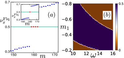
Figure 3: (Color online) (a) Floquet Wannier Spectrum (FWS) is demonstrated for $B_{x}=0$ and the inset manifests the same for $B_{x}=0.3$. The values of all other parameters remain the same as in Fig. 2. Connecting with Fig. 2, we can comment that eight (four) MCMs correspond to four (two) FWS quantized at $0.5$. We refer the phase with eight and four MCMs as weak and strong FSOTSC phases, respectively. (b) Floquet Quadrupole moment (FQM), which is only quantized at $0.5$ for the strong FSOTSC phase, is demonstrated in $m_{1}$-$\omega$ plane where $m_{1}$ and $\omega$ are the amplitude of the drive and the driving frequency respectively.

In order to calculate the FQM, being another invariant for the quantification of the topological phases, we numerically diagonalize the exact Floquet operator (Eq.(3)). We then construct the Floquet many-body ground state $\Psi_{0,\rm F}$ by columnwise marshalling the quasi-states according to their quasi-energy $-\omega/2\leq\mu_{m}\leq 0$: $\Psi_{0,\rm F}=\sum_{m\in\mu_{m}\leq 0}|\phi_{m}\rangle\langle\phi_{m}|$ Nag et al. (2019); Ghosh et al. (2020). Now $Q^{\rm Flq}_{xy}(r)$ can be defined, considering the geometrical number operator ${\hat{q}}_{xy}={\hat{n}}(r)xy/L^{2}$ with ${\hat{n}}(r)$ being the number operator at $r=(x,y)$, as follows

$$Q^{\rm Flq}_{xy} = {\rm Re}\left[-\frac{i}{2\pi}{\rm Tr}\left(\ln\Big{(}\Psi_{0,\rm F}^{\dagger}\exp\Big{[}2\pi i\sum_{r}{\hat{q}}_{xy}(r)\Big{]}\Psi_{0,\rm F}\Big{)}\right)\right].$$

For $B_{x}\neq 0$, we obtain $Q^{\rm Flq}_{xy}\equiv{\rm mod}(Q^{\rm Flq}_{xy},1)=0.5$. On the other hand, when $B_{x}=0$, $Q^{\rm Flq}_{xy}$ turns out to be zero, depicting weak topological nature of the phase. Therefore, similar to the FWS, we here also find finite (vanishing) FQM for strong (weak) FSOTSC phases. We then explore the dynamic FSOTSC phase for a range of the driving frequency $\omega$ and the driving amplitude $m_{1}$ where $Q^{\rm Flq}_{xy}=0.5$. This is shown in Fig. 3(b). This clearly suggests that the emergent strong phase is indeed an outcome of non-equilibrium dynamics as the underlying static model remains in a non-topological phase.

III Majorana Hinge modes in 3d

In this section we generalize our earlier findings of FSOTSC phase in case of 3D.

III.1 Model Hamiltonian and Driving Protocol

III.1.1 Model

In 3D, we begin by writting down the Hamiltonian in the Bogoliubov-de Gennes (BdG) form as $H_{\rm BdG}=\sum_{{\bm{\mathrm{k}}}}\Psi^{\dagger}_{\bm{\mathrm{k}}}\mathcal{H}^{\rm 3D}_{0}({\bm{\mathrm{k}}})\Psi_{\bm{\mathrm{k}}}$, with $\Psi_{\bm{\mathrm{k}}}=\left(c_{{\bm{\mathrm{k}}},a\uparrow},-c_{-{\bm{\mathrm{k}}},a\downarrow}^{\dagger},c_{{\bm{\mathrm{k}}},a\downarrow},c_{-{\bm{\mathrm{k}}},a\uparrow}^{\dagger},c_{{\bm{\mathrm{k}}},b\uparrow},-c_{-{\bm{\mathrm{k}}},b\downarrow}^{\dagger},c_{{\bm{\mathrm{k}}},b\downarrow},c_{-{\bm{\mathrm{k}}},b\uparrow}^{\dagger}\right)^{\tilde{T}}$ and $\mathcal{H}^{\rm 3D}_{0}({\bm{\mathrm{k}}})$ is given by

$$\mathcal{H}^{\rm 3D}_{0} = \epsilon(\bm{\mathrm{k}})\Gamma_{1}+\lambda_{x}\sin k_{x}\Gamma_{2}+\lambda_{y}\sin k_{y}\Gamma_{3}+\lambda_{z}\sin k_{z}\Gamma_{4}$$

$$+\Delta(\bm{\mathrm{k}})\Gamma_{5}+B_{x}\Gamma_{6}+B_{y}\Gamma_{7}+B_{z}\Gamma_{8}\equiv{\bm{\mathrm{N}}}(\bm{\mathrm{k}})\cdot{\bm{\Gamma}}\ ,$$

where, $\epsilon(\bm{\mathrm{k}})=\left(m_{0}-t_{x}\cos k_{x}-t_{y}\cos k_{y}-t_{z}\cos k_{z}\right)$, $\Delta(\bm{\mathrm{k}})=\Delta\left(\cos k_{x}-\cos k_{y}\right)$ and $\Gamma_{1}=\sigma_{z}\tau_{z}$, $\Gamma_{2}=\sigma_{x}s_{x}\tau_{z}$, $\Gamma_{3}=\sigma_{x}s_{y}\tau_{z}$, $\Gamma_{4}=\sigma_{x}s_{z}\tau_{z}$, $\Gamma_{5}=\tau_{x}$, $\Gamma_{6}=s_{x}$, $\Gamma_{7}=s_{y}$ and $\Gamma_{8}=s_{z}$. Similar to the Hamiltonian (Eq.(1)) in 2D case, $\mathcal{H}^{\rm 3D}_{0}$ respects both TRS $\mathcal{T}=is_{y}\mathcal{K}$ and PHS $\mathcal{C}=s_{y}\tau_{y}\mathcal{K}$ in absence of Zeeman field i.e.,  $B_{x}=B_{y}=B_{z}=0$. In absence of the superconducting term $\Delta(\bm{\mathrm{k}})=0$, the model supports zero-energy surface states for $|m_{0}|<t_{x}+t_{y}+t_{z}$. While for $|m_{0}|>t_{x}+t_{y}+t_{z}$, the models becomes non-topological (trivial band insulator). This model thus supports the first order topological phase in the absence of $\Delta(\bm{\mathrm{k}})$. Interestingly, the model becomes a PHS protected SOTSC, hosting MKPs at the hinges along $z$ direction, in the presence of $\Delta(\bm{\mathrm{k}})$ when $|m_{0}|<t_{x}+t_{y}+t_{z}$. In case of 2D system (Eq. (1)), the SOTSC phase supports MCMs; here for 3D system (Eq. (LABEL:ham3D)), it hosts Majorana hinge modes (MHMs). Upon breaking TRS by introducing magnetic field $B_{x}\neq 0$, the degeneracy of MKPs get lifted and there exist only one MZM per hinge. We note that $B_{y}$ does the same job as done by $B_{x}$. In contrast, $B_{z}$ is not able to lift the degeneracy of MKPs. In general, the MHMs are observed along $c$ direction when the SC order has the form $\Delta(\bm{\mathrm{k}})=\cos k_{a}-\cos k_{b}$ with $a,b,c=x,y,z$. The MKPs along the hinges in the $c$ direction remain unaffected by the magnetic field $B_{c}$. On the other hand, for $|m_{0}|>t_{x}+t_{y}+t_{z}$, the system continues to remain in the non-topological phases even with $\Delta(\bm{\mathrm{k}})\neq 0$ and $B_{x}\neq 0$. Therefore, it would be interesting to study the generation of FSOTSC phase in presence of $\Delta$ by kicking the mass term while the underlying static system remains in a non-topological phase. Our aim is to generate the Floquet MHMs (FMHMs) and their topological characterization in 3D geometry.

III.1.2 Driving Protocol and Floquet Operator

We consider the same driving protocol in the form of periodic kick as followed in the 2D case where

$$m(t) = m_{1}\sum_{r=1}^{\infty}\delta(t-rT)\ .$$ (32)

Here, $T$ is the period of the drive and $m_{1}$ is the amplitude of the drive. With the periodic kick (see Eq.(32)), the Floquet operator reads

$$U(T) = {\rm\bf TO}\exp\left[-i\int_{0}^{T}dt\left(\mathcal{H}^{\rm 3D}_{0}(\bm{\mathrm{k}})+m(t)\Gamma_{1}\right)\right]$$ (33)

$$= \exp(-i\mathcal{H}^{\rm 3D}_{0}(\bm{\mathrm{k}})T)~{}\exp(-im_{1}\Gamma_{1})\ .$$

We can cast the Floquet Operator $U(T)$ in a more compact form as

$$U(T) = C_{T}\left(p-iq\Gamma_{1}\right)-iS_{T}\sum_{j=1}^{8}\left(n_{j}\Gamma_{j}+m_{j}\Gamma_{j1}\right),\ \$$ (34)

where, $C_{T}=\cos(\left|{\bm{\mathrm{N}}}(\bm{\mathrm{k}})\right|T)$, $S_{T}=\sin(\left|{\bm{\mathrm{N}}}(\bm{\mathrm{k}})\right|T)$, $p=\cos m_{1}$, $q=\sin m_{1}$, $n_{j}=\frac{N_{j}(\bm{\mathrm{k}})\cos m_{1}}{\left|{\bm{\mathrm{N}}}(\bm{\mathrm{k}})\right|}$, $m_{j}=\frac{N_{j}(\bm{\mathrm{k}})\sin m_{1}}{\left|{\bm{\mathrm{N}}}(\bm{\mathrm{k}})\right|}$ and $\Gamma_{j1}=\frac{1}{2i}\left[\Gamma_{j},\Gamma_{1}\right]$ with $j=2,3,4,5,6,7,8$. One can find the general form of the effective Hamiltonian as

$$H_{\rm Flq}=\frac{\xi_{\bm{\mathrm{k}}}}{\sin\xi_{\bm{\mathrm{k}}}T}\Bigg{[}\sin(\left|{\bm{\mathrm{N}}}(\bm{\mathrm{k}})\right|T)\cos m_{1}\sum_{j=1}^{8}r_{j}\Gamma_{j}+\cos(\left|{\bm{\mathrm{N}}}(\bm{\mathrm{k}})\right|T)\sin m_{1}\Gamma_{1}+\sin(\left|{\bm{\mathrm{N}}}(\bm{\mathrm{k}})\right|T)\sin m_{1}\sum_{j=2}^{8}r_{j}\Gamma_{j1}\Bigg{]}\ ,$$ (35)

with $\xi_{\bm{\mathrm{k}}}=\frac{1}{T}\cos^{-1}\left[\cos(\left|{\bm{\mathrm{N}}}(\bm{\mathrm{k}})\right|T)\cos m_{1}\right]$, $r_{j}=\frac{N_{j}(\bm{\mathrm{k}})}{\left|{\bm{\mathrm{N}}}(\bm{\mathrm{k}})\right|}$. In the high-frequency limit i.e.,   $T\rightarrow 0$ and $m_{1}\rightarrow 0$, neglecting the higher order terms in $T$ and $m_{1}$, we find the effective Hamiltonian as

$$H_{\rm Flq}\approx\mathcal{H}_{0}(\bm{\mathrm{k}})+\frac{m_{1}}{T}\Gamma_{1}+m_{1}\sum_{j=2}^{8}r_{j}\Gamma_{j1}\ ,$$ (36)

In Eq.(36), terms associated with $\Gamma_{j1}$ are the new terms generated by the drive. Note that these new terms break TRS $\mathcal{T}$ present in the static Hamiltonian. Although $H_{\rm Flq}$ continues to preserve the anti-unitary PHS $\mathcal{C}$. Similar to the 2D case as described by Eq.(6), here also the extra terms $r_{j}\Gamma_{j1}$ break the TRS of the model even when $B_{x}=B_{y}=B_{z}=0$. The Hamiltonian (Eq.(36)) shares similar characteristics as shown by the 2D Hamiltonian (Eq.(6)). Here also the mass term is renormalized to $m_{0}\to(m_{0}+m_{1}/T)$ and the topological phase boundary becomes accordingly modified. The dynamical (explicit) breaking of TRS would lead to an interesting study as far as the weak (strong) FSOTSC phases are concerned. As noted in the static case, the in-plane Zeeman field $B_{x}$ or $B_{y}$ can lead to an interesting effect for the Floquet case also.

III.2 Floquet Majorana Hinge Mode

Here, we numerically diagonalize the Floquet operator (Eq.(33)) in real space geometry to manifest the signature of the 1D propagating MHMs along the $z$-direction in the LDOS spectrum. Like before, we consider two cases. When the Zeeman field $\bm{\mathrm{B}}=0$, we obtain eight eigenvalues close to zero-energy like the 2D case as shown in Fig. 4(b). However, when we incorporate $B_{x}\neq 0$ or $B_{y}\neq 0$, we obtain four modes near zero-energy (see Fig. 4(b)I2). Interestingly, the transverse magnetic field $B_{z}$ does not give rise to these kinds of phenomena. However, the finite-size effect is very prominent here that we depict in the inset I1 of Fig. 4(b). The finite-size gap $\Delta_{G}$ vanishes exponentially with $L$: $\Delta_{G}\sim\beta\exp(-\alpha L)$. This ensures the fact that MHMs are indeed zero-energy FSOTSC states in 3D. We show the LDOS explicitly in Fig. 4(a) where one can observe that a finite spectral weight is uniformly distributed over the four hinges of the 3D cubic system.

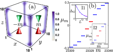
Figure 4: (Color online) (a) The LDOS associated with the MZMs clearly exhibits the emergence of the 1D Floquet MHMs in finite geometry. The LDOS structure remains qualitatively invariant in the presence of an in-plane Zeeman field. We choose the other parameter values as $t_{x}=t_{y}=t_{z}=2.0$, $\lambda_{x}=\lambda_{y}=\lambda_{z}=1.0$, $m_{0}=5.5$, $m_{1}=-0.3$ and $T=0.393$. (b) The Floquet quasi-energy spectra is shown for the 3D FSOTSC in real space without the Zeeman field. There exist eight MHMs (due to the finite size effect, these modes do not appear exactly at zero energy) referring to the fact that this is a weak phase where each hinge is occupied by two MZMs. The finite-size effect is investigated in the inset I1 showing the gap as a exponentially falling function of the system size in one real space direction as $\Delta_{G}\sim\beta\exp(-\alpha L)$ with $\alpha=0.127283$ and $\beta=0.769069$. With Zeeman field $B_{x}=0.4$, we depict (inset I2) the emergence of four MHMs i.e., one MZM per hinge. The Zeeman field can thus transform a weak FSOTSC to a strong FSOTSC phase.

III.3 Low energy surface theory

We here investigate the low-energy theory for 3D case to search for the existence of the hinge states, originated due to periodically kicked mass term, in the underlying static Hamiltonian (Eq.(LABEL:ham3D)). For simplicity we choose $t_{x}=t_{y}=t_{z}=t$ and $\lambda_{x}=\lambda_{y}=\lambda_{z}=\lambda$. We expand the high-frequency effective Hamiltonian (Eq.(36)) around $\Gamma=(0,0,0)$ point and obtain

$$H_{\rm Flq,\Gamma}^{\rm 3D} = \left(m^{\prime}+\frac{t}{2}\partial_{x}^{2}+\frac{t}{2}\partial_{y}^{2}+\frac{t}{2}\partial_{z}^{2}\right)\Gamma_{1}+\lambda k_{x}\Gamma_{2}$$

$$+\lambda k_{y}\Gamma_{3}+\lambda k_{z}\Gamma_{4}-\frac{\Delta}{2}\left(k_{x}^{2}-k_{y}^{2}\right)\Gamma_{5}+\frac{m_{1}}{T}\Gamma_{1}$$

$$+m_{1}\lambda k_{x}\Gamma_{21}+m_{1}\lambda k_{y}\Gamma_{31}+m_{1}\lambda k_{z}\Gamma_{41}$$

$$-\frac{m_{1}\Delta}{2}\left(k_{x}^{2}-k_{y}^{2}\right)\Gamma_{51}+B_{x}\Gamma_{6}+B_{y}\Gamma_{7}+B_{z}\Gamma_{8},$$

where, $m^{\prime}=(m_{0}-3t)$ and $\Gamma_{21}=-\sigma_{y}s_{x}$, $\Gamma_{31}=-\sigma_{y}s_{y}$, $\Gamma_{41}=-\sigma_{y}s_{z}$ and $\Gamma_{51}=-\sigma_{z}\tau_{y}$. We choose a surface perpendicular to the $xy$-plane, with a deviation from $yz$-plane by an angle $\theta$. In order to cast the above equations in a convenient form we translate to a rotated frame defined by $k_{1}=-\sin\theta~{}k_{x}+\cos\theta~{}k_{y}$, $k_{2}=k_{z}$ and $k_{3}=\cos\theta~{}k_{x}+\sin\theta~{}k_{y}$. This rotation transforms $x,~{}y,~{}z\to~{}y,~{}z,~{}x$ for $\theta=0$ while for $\theta=\pi/2$, $x,~{}y,~{}z\to-x,~{}z,~{}y$. We now consider OBC in the $x_{3}$ direction and replace $k_{3}\rightarrow-i\partial_{3}$. One can hence divide Eq.(LABEL:3dlow1) into two parts as

$$H_{0} = \left(m-\frac{t}{2}\partial_{3}^{2}\right)\sigma_{z}\tau_{z}-i\lambda\partial_{3}\ \sigma_{x}\left(s_{x}\cos\theta+s_{y}\sin\theta\right)\tau_{z},$$

$$H_{p} = \lambda k_{1}\sigma_{x}\left(-s_{x}\sin\theta+s_{y}\cos\theta\right)\tau_{z}+\lambda k_{2}\sigma_{x}s_{z}\tau_{z}$$ (38)

$$-\frac{\Delta(\theta)}{2}\partial_{3}^{2}\ \tau_{x}+im_{1}\lambda\partial_{3}\sigma_{y}\left(s_{x}\cos\theta+s_{y}\sin\theta\right)$$

$$-m_{1}\lambda k_{1}\sigma_{y}\left(-s_{x}\sin\theta+s_{y}\cos\theta\right)-m_{1}\lambda k_{2}\sigma_{y}s_{z}$$

$$+\frac{m_{1}\Delta(\theta)}{2}\partial_{3}^{2}\ \sigma_{z}\tau_{y}+B_{x}s_{x}+B_{y}s_{y}+B_{z}s_{z}\ ,$$

where, $m=\left(m^{\prime}+\frac{m_{1}}{T}\right)$ and $\Delta(\theta)=\Delta\left(\sin^{2}\theta-\cos^{2}\theta\right)$. We consider the following transformation for spins

$$\begin{pmatrix}s_{x}\\ s_{y}\\ s_{z}\end{pmatrix}=\begin{pmatrix}-\sin\theta&\cos\theta&0\\ \cos\theta&\sin\theta&0\\ 0&0&1\end{pmatrix}\begin{pmatrix}s_{1}\\ s_{3}\\ s_{2}\end{pmatrix}$$ (39)

such that Eq.(38) acquires a compact form as we notice for 2D case. Here, $s_{1}$, $s_{2}$ and $s_{3}$ are Pauli matrices. Therefore, Eq.(38) can be rewritten as

$$H_{0} = \left(m-\frac{t}{2}\partial_{3}^{2}\right)\sigma_{z}\tau_{z}-i\lambda\partial_{3}\ \sigma_{x}s_{3}\tau_{z},$$

$$H_{p} = \lambda k_{1}\sigma_{x}s_{1}\tau_{z}+\lambda k_{2}\sigma_{x}s_{2}\tau_{z}-\frac{\Delta(\theta)}{2}\partial_{3}^{2}\ \tau_{x}+im_{1}\lambda\partial_{3}\sigma_{y}s_{3}$$ (40)

$$-m_{1}\lambda k_{1}\sigma_{y}s_{1}-m_{1}\lambda k_{2}\sigma_{y}s_{2}+\frac{m_{1}\Delta(\theta)}{2}\partial_{3}^{2}\ \sigma_{z}\tau_{y}$$

$$+B_{x}\left(-s_{1}\sin\theta+s_{3}\cos\theta\right)+B_{y}\left(s_{1}\cos\theta+s_{3}\sin\theta\right)$$

$$+B_{z}s_{2}\ \ ,$$

We assume $\Psi$ to be zero-energy solution of $H_{0}$ with the boundary condition $\Psi(x_{3}=0)=\Psi(x_{3}=\infty)=0$. We finally obtain the following wave-function in the rotated frame as

$$\Psi_{\alpha}=A\ e^{-\mathcal{K}_{1}x_{3}}\sin(\mathcal{K}_{2}x_{3})\ e^{ik_{1}x_{1}+ik_{2}x_{2}}\ \Phi_{\alpha},$$ (41)

where, $\mathcal{K}_{1}=\frac{\lambda}{t}$, $\mathcal{K}_{2}=\sqrt{\lvert\frac{2m}{t}\rvert-\mathcal{K}_{1}^{2}}$ and $A=\frac{4\mathcal{K}_{1}\left(\mathcal{K}_{1}^{2}+\mathcal{K}_{2}^{2}\right)}{\mathcal{K}_{2}^{2}}$ and $\Phi_{\alpha}$ is $8$-component spinor satisfying $\sigma_{y}s_{3}\Phi_{\alpha}=-\Phi_{\alpha}$.

$$\Phi_{1} = \ket{\sigma_{y}=+1}\otimes\ket{s_{3}=-1}\otimes\ket{\tau_{z}=+1},$$

$$\Phi_{2} = \ket{\sigma_{y}=-1}\otimes\ket{s_{3}=+1}\otimes\ket{\tau_{z}=+1},$$

$$\Phi_{3} = \ket{\sigma_{y}=+1}\otimes\ket{s_{3}=-1}\otimes\ket{\tau_{z}=-1},$$

$$\Phi_{4} = \ket{\sigma_{y}=-1}\otimes\ket{s_{3}=+1}\otimes\ket{\tau_{z}=-1}\ .$$ (42)

The matrix element of $H_{p}$ in the rotated frame within the above basis reads

$$H_{\alpha\beta}^{\rm Surf}=\int_{0}^{\infty}dx_{3}\ \Psi_{\alpha}^{\dagger}(x_{3})H_{p}\Psi_{\beta}(x_{3})\ .$$ (43)

Therefore, we obtain the Hamiltonian for the surface in the rotated frame to be

$$H^{\rm Surf}=\lambda k_{1}s_{3}\tau_{y}-\lambda k_{2}s_{3}\tau_{x}+M(\theta)s_{1}-B(\theta)\tau_{z}\ .$$ (44)

Here, $M(\theta)=\Delta(\theta)\lvert\frac{m}{t}\rvert$ and $B(\theta)=\left(B_{x}\cos\theta+B_{y}\sin\theta\right)$. The transverse magnetic field $B_{z}$ does not appear in the surface Hamiltonian referring to the fact that in-plane magnetic field plays the important role in determining the nature of the FSOTSC phase. Interestingly, $\Delta(\theta)=-\Delta(\theta+\pi/2)$ resulting in $M(\theta)$ to change its sign between two adjacent surfaces under $C_{4}$ rotation around $z$ axis. Consequently, one can get hinge mode in the junction between $xz$- and $yz$-plane. This sign change of the mass term is shown in Fig. 4 (a). We can explicitly write down the surface Hamiltonian for the $yz$ ($xz$) -surface by putting $\theta=0~{}(\frac{\pi}{2})$ as

$$H^{yz} = \lambda k_{y}s_{3}\tau_{y}-\lambda k_{z}s_{3}\tau_{x}-\Delta\left|\frac{m}{t}\right|s_{1}-B_{x}\tau_{z}\ ,$$

$$H^{xz} = -\lambda k_{x}s_{3}\tau_{y}-\lambda k_{z}s_{3}\tau_{x}+\Delta\left|\frac{m}{t}\right|s_{1}-B_{y}\tau_{z}\ .\quad$$ (45)

Let us now discuss the above surface Hamiltonian at length. As compared to the edge Hamiltonian for edge-$a$ with $k_{a}$ only, surface Hamiltonian for $ab$ surface consists of $k_{a}$ and $k_{b}$. In the absence of magnetic field, $\Delta\left|\frac{m}{t}\right|s_{1}$ acts as a mass in the Nambu space spanned by $s_{3}\tau_{x,y}$. This mass changes its sign between two adjacent surfaces namely, $yz$ and $xz$. Both the blocks participate actively here as the mass term uniformly appears in both of them. Thus two MZMs per hinge are observed. On the other hand, in the presence of any of the in-plane Zeeman field, mass terms become different in the two blocks. This leads to a situation where one block can be made active keeping the other block inactive. As a result, one MZMs per hinge can be observed. This behavior is again in resemblance with that of the 2D case. Therefore, the dynamical and explicit breaking of TRS imprints their signatures unanimously for 3D as well.

III.4 Hinge Mode Solution

Having obtained low energy surface Hamiltonian, the hinge Hamiltonian can be estimated by considering the PBC (OBC) along (perpendicular to) hinge direction. We thus divide $H^{\rm Surf}$ into two parts as

$$H_{0}^{S} = -i\lambda\partial_{1}s_{3}\tau_{y}+M(\theta)s_{1}-B(\theta)\tau_{z}\ ,$$

$$H^{S}_{p} = -\lambda k_{2}s_{3}\tau_{x}\ ,$$ (46)

Here the superconducting order parameter and Zeeman field are treated in the unperturbed Hamiltonian $H_{0}^{S}$. We solve $H_{0}^{S}$ exactly and expand $H^{S}_{p}$ in the basis of $H^{S}_{0}$. For $\bm{\mathrm{B}}=0$, we obtain the Hamiltonian for the hinge mode (after replacing $k_{2}\rightarrow k_{z}$) as

$$H^{\rm Hinge}=-\lambda k_{z}\tau_{y}\ ,$$ (47)

This manifests a propagating mode along $z$ direction. Therefore, it clear that dynamical breaking of TRS leads to two solutions of MHMs with $\tau_{y}=\pm 1$. Contrastingly for $B_{x}\neq 0$ or $B_{y}\neq 0$, we obtain the solution as

$$H^{\rm Hinge}=-\lambda k_{z}\mathbb{I}\ ,$$ (48)

which only hosts a single MHM as the hinge Hamiltonian is described by $\mathbb{I}$. Similar to the 2D case, here also the explicit breaking of TRS can lead to a situation different from the dynamical breaking of TRS by the periodic kick drive. Hence, one expects that without (with) magnetic field there exist two MHMs (one MHM) per hinge along $z$ direction as shown in the inset I2 of Fig. 4(b).

III.5 Floquet Wannier Spectrum

To calculate FWS using Eq.(28), we write down the Hamiltonian (Eq.(LABEL:ham3D)) in slab geometry i.e.,  we consider OBC in one direction while the other two directions continue to satisfy PBC. For a $x$-directed slab (OBC along $x$-direction; PBC along $y$ and $z$-direction), we can calculate $\nu_{z}^{(x),\rm Flq}$ ($\nu_{y}^{(x),\rm Flq}$) as a function of $k_{y}$ ($k_{z}$). Since we obtain propagating 1D hinge mode in $z$ direction only, the spectrum of $\nu_{y}^{(x),\rm Flq}$ and $\nu_{x}^{(y),\rm Flq}$ as a function of $k_{z}$ exhibits gapless nature, while all other FWS remain gapped. We illustrate the representative plots for FWS in Figs. 5(a)-(b). Focussing only at $k_{z}=0$ point, we show FWS as a function of the state-index at $k_{z}=0$ in Figs. 5(c)-(d). In absence of the in-plane Zeeman field i.e.,  for weak FSOTSC phase, we obtain four eigenvalues at 0.5 correspondings to the two MHMs per hinge (see Fig. 5(c)). In contrast, when we turn on the in-plane Zeeman field, $B_{x}$ i.e.,  for strong FSOTSC, we obtain two eigenvalues at 0.5 (see Fig. 5(d)) corroborating one MHM per hinge. We also calculate the FQM to further distinguish between the weak and strong FSOTSC. To proceed, we write the Floquet operator $U(T)$ (Eq.(33)) in rod geometry (considering PBC along $z$-direction, OBC along $x$ and $y$-direction). We then implement Eq.(LABEL:qm_xy) to calculate the FQM ($Q_{xy}^{\rm Flq}$) as a function of $k_{z}$. We find that $Q_{xy}^{\rm Flq}=0.5~{}(0)$ at $k_{z}=0$ for the strong (weak) phase Fu et al. .

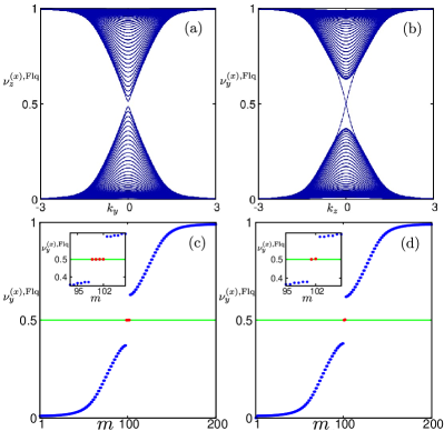
Figure 5: (Color online) (a) We depict the FWS $\nu_{z}^{(x),\rm Flq}$ as a function of $k_{y}$ in the slab geometry with OBC along $x$ direction and PBC along $y$, $z$ directions. (b) We work in the same geometry as mentioned in panel (a) but show $\nu_{y}^{(x),\rm Flq}$ as a function of $k_{z}$. Since, the hinge mode propagates along $z$-direction, we obtain gapless FWS for $\nu_{y}^{(x),\rm Flq}$. (c) We show the FWS $\nu_{y}^{(x),\rm Flq}$ as a function of state number at $k_{z}=0$ for $B_{x}=0$. In the inset one can clearly observe four eigenvalues at $0.5$ refer to the weak FSOTSC phase. (d) We repeat (c) but with the in-plane Zeeman field $B_{x}\neq 0$. We obtain two eigenvalue at $0.5$ as shown in the inset refer to strong FSOTSC phase. The values of all the parameter remain same as in Fig. 4.

IV Robustness of higher order Majorana modes against disorder

Having investigated the topological classification of the FSOTSC phases, we now focus on the robustness of these phases in presence of finite disorder. We first concentrate on the 2D case. Instead of choosing $m_{1}$ to be constant, we consider $m_{1}$ to be randomly distributed in between $\left[-\frac{W}{2},\frac{W}{2}\right]$ in an un-correlated manner. Here, $W$ being the strength of the disorder. Note that, the disorder being random, we have taken average over $500$ disorder configurations in our numerical calculation. We analyze our results for two values of disorder strengths, $W=0.1$ and $0.4$ while hopping and spin-orbit coupling strength is fixed to unity. We first study the effect of disorder on the weak phase hosting eight MCMs. For weak disorder strength, $W=0.1$, one does not observe any perceptible difference from the clean case (see Fig. 6(a)). To be precise, the spectral weight of MCMs are uniformly distributed among all the four corners of the square lattice i.e.,  the localization length remains almost unaltered in presence of weak disorder. While for $W=0.4$, we notice that the spectral weight of some corner modes in LDOS becomes higher compared to other as shown in Fig. 6(b). This non-uniform distribution of spectral weight among the corners thus suggests that the strong disorder can substantially modify the localization properties of these MCMs. However, it is noteworthy that even strong disorder cannot lift the Majorana modes from the zero-energy as depicted in the inset of Figs. 6(a) and (b). This results in the fact that FWS continues to exhibit similar behavior as compared to the clean case (see Figs. 7(a) and (b)). Therefore, weak FSOTSC phase can preserve its signature in the presence of moderate disorder.

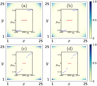
Figure 6: (Color online)(a) LDOS, associated with zero quasi-energy states $\mu_{m}=0$, in finite geometry is demonstrated for $B_{x}=0$ and inset shows the Floquet quasi-energy spectrum for the same for the disorder strength $W=0.1$. (b) We repeat (a) with the disorder strength $W=0.4$. (c) and (d), we repeat (a) and (b) with $B_{x}=0.3$, respectively. One can clearly observe that the localization properties become modified as the disorder strength increases substantially, otherwise for small disorder, they remain same as the clean case. Value of all other parameters remain same as in Fig. 2.

We also investigate the effect of moderate disorder in the strong FSOTSC phase hosting four MZMs at the corners in the presence of explicit TRS breaking Zeeman field. Since the disorder does not break any further symmetry (except translational), we find that the effect of the disorder remains same as the earlier case with $B_{x}=0$. The uniform (non-uniform) distribution of spectral weight of MZMs is observed for $W=0.1$ ($0.4$) as depicted in Fig.  6(c) and (d). These MCMs are localized at zero-energy always (see the inset of Fig. 6(c) and (d)). As a result, their topological protection remains unaltered as noticed in the clean case. We find quantized FWS for weak as well as moderate disorder strength (see the inset of Figs. 7(a) and (b)). It is important to mention that the FQM is also quantised at a value $0.5$, for such strength of the disorder with $B_{x}\neq 0$. This investigation with moderate disorder thus clearly suggests that bothweak and strong FSOTSC phases are robust against moderate disorder. Having investigated the effect of disorder and protection of topological properties in 2D, we believe the same line of argument would also hold for 3D.

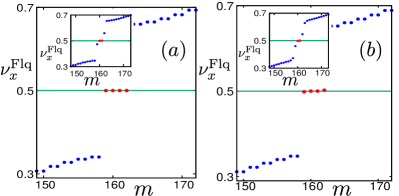
Figure 7: (Color online) (a) FWS is depicted for the case $B_{x}=0$ when the disorder strength is chosen to be $W=0.1$, while the same for the case $B_{x}=0.3$ is shown in the inset. (b) FWS is demonstrated with the disorder strength $W=0.4$ for $B_{x}=0$ and $B_{x}\neq 0$ (inset). One can obtain an indication that upon increasing the disorder strength substantially, the FWS might deviate from the quantized value $0.5$. However, for our chosen disorder strength ($W<t_{x},t_{y},\lambda_{x},\lambda_{y}$) the invariant behaves in robust manner referring to the fact that these FSOTSC phases are stable against moderate disorder. Value of all the other parameters remain same as chosen in Fig. 2.

V Summary and Conclusions

To summarize, in this article, we provide a dynamical prescription to generate the FSOTSC phase starting from a 2D/3D TI in close proximity to an unconventional $d$-wave superconductor. We periodically kick the mass term to generate MZMs at the corners and hinges in 2D square and 3D cubic lattice geometry, respectively. Our aim here is to investigate the effect of TRS breaking magnetic field on these Floquet SOTSC phases as the initial (effective) Hamiltonian, describing the static (driven) system which preserves (breaks) the dynamical TRS. In 2D, we first consider our model in the presence of periodically kicked mass term when Zeeman field $B_{x}=0$. Here, we find FSOTSC phase harboring eight MZMs i.e.,  two MZMs per corner. In order to characterize this FSOTSC phase, we compute two topological invariants namely, FWS and FQM. We find that this phase corresponds to four FWS quantized at $0.5$ while FQM vanishes; we identify this FSOTSC phase as the weak one. Upon introduction of an explicit TRS breaking Zeeman field $B_{x}\neq 0$, we find four MZMs i.e.,  one MZM per corner. We here obtain two quantized FWS at $0.5$ and quantized FQM referring to the strong nature of the phase. We analytically support our numerical findings, as obtained by diagonalizing the Floquet operator in OBC, with the help of effective low-energy edge theory and MCMs solutions. The low-energy theory can successfully predict the nature of the SOTSC phase whether it is strong or weak in terms of the spinor states of MZMs. We further introduce moderate disorder in the driving amplitude to study the stability of the FSOTSC phase against disorder. We find that the FSOTSC is stable against the moderate strength of disorder. However, the localization property of the MZMs depends on the disorder strength. We also generalize our theory based on 3D model and identify the weak (strong) FSOTSC phase via FWS hosting MHMs. In this case, we derive the low energy surface theory and analytical solutions of the MHMs therein. The effect of the disorder remains similar as in 2D case.

As far as experimental feasibility of our setup is concerned, $d$-wave superconductivity in TI can be induced via the proximity effect (e.g., $\rm Bi_{2}Sr_{2}CaCu_{2}O_{8+\delta}$) Wang et al. (2013b) with an induced gap amplitude $\Delta\sim 15~{}\rm meV$ Wang et al. (2013b). It has been theoretically Liu et al. (2010) and experimentally Zhang et al. (2010) demonstrated that the topological properties of (Bi,Sb)₂Te₃ thin films can be tuned by the quantum confinement i.e.,  varying the number of quintuple layers. It is indeed possible to tune the mass term in the underlying static model which might pave the way to realize the dynamical manipulation of mass term in the proximized topological superconductor. In recent times, experimental advancements on the pump-probe techniques Wang et al. (2013a); Maczewsky et al. (2017); Peng et al. (2016) have enabled one to observe Floquet topological insulators Wang et al. (2013a) and anomalous Hall effect in graphene McIver et al. (2020).Therefore, we believe that the signature of MCMs and MHMs may be possible to achieve via pump-probe based time-resolved transport (e.g., local scanning tunneling microscope (STM)) measurements Nadj-Perge et al. (2014); Sato et al. (2019); Tuovinen et al. (2019) for an in-plane magnetic field $B_{x}\sim 7-8~{}\rm T$, amplitude of the drive $m_{1}\sim 100~{}\rm meV$ and period $T\sim 2~{}\rm fs$.

At last, we would like to comment on robustness of these Floquet MZMs in HOTSC phases under periodic driving as far as heating and dissipation are concerned. Based on the recent theoretical and experimental investigations on quantum many-body systems Abanin et al. (2015); Messer et al. (2018), the heating is suppressed in the prethermal window where our findings can be tested with dissipationless MZMs associated with the periodic steady state. We work in the high frequency regime away from the resonance points. This further enables us to minimize the heating effect Bukov et al. (2015). We therefore believe that our theoretical findings do not suffer from heating issue and dissipation.