Abstract

Users of recommender systems often behave in a non-stationary fashion, due to their evolving preferences and tastes over time. In this work, we propose a practical approach for fast personalization to non-stationary users. The key idea is to frame this problem as a latent bandit, where the prototypical models of user behavior are learned offline and the latent state of the user is inferred online from its interactions with the models. We call this problem a non-stationary latent bandit. We propose Thompson sampling algorithms for regret minimization in non-stationary latent bandits, analyze them, and evaluate them on a real-world dataset. The main strength of our approach is that it can be combined with rich offline-learned models, which can be misspecified, and are subsequently fine-tuned online using posterior sampling. In this way, we naturally combine the strengths of offline and online learning.

1 Introduction

When users interact with recommender systems or search engines, their behavior is often guided by a latent state, a context that cannot be observed. Examples of latent states are user preferences, which persist over longer periods of time, and shorter-term user intents. As the users interact, their latent state is slowly revealed by their responses. A good recommender should cater to the user based on the latent state, which first needs to be discovered.

We formalize the problem of recommending to a user under a changing latent state as a multi-armed bandit (Lai and Robbins, 1985; Auer, 2002; Lattimore and Szepesvári, 2019). In this setting, the recommender is a learning agent and its actions are the arms of a bandit. After an arm is pulled, the agent observes a response from the user, which is also its reward. The response is a function of the observed context and an unobserved latent state. The goal of the learning agent is to maximize its cumulative reward over $n$ interactions with the user. The challenge is that the latent state of the user is unobserved and changes. This setting is known as piecewise-stationary bandits (Hartland et al., 2007; Garivier and Moulines, 2008; Yu and Mannor, 2009).

Both non-stationary bandits (Auer et al., 2002b; Luo et al., 2018) and the special case of piecewise-stationary bandits (Hartland et al., 2007; Garivier and Moulines, 2008; Yu and Mannor, 2009) have been studied extensively in prior work. The main departures in this work are two fold. First, we assume that the latent state changes stochastically. Second, we assume that the learning agent knows, at least partially, the reward models of arms conditioned on each latent state. This assumption is realistic in most recommender domains, where a plethora of offline data allow for rich models of user behavior, conditioned on the user type, to be learned offline. Under these assumptions, the problem of learning to act can be solved efficiently by Thompson sampling (TS) (Thompson, 1933; Chapelle and Li, 2012; Russo and Van Roy, 2013) over latent states, which we propose, analyze, and extensively evaluate. To the best of our knowledge, this is the first analysis of TS in this highly practical setting.

Our approach has many benefits over prior works. Unlike adversarial techniques (Auer et al., 2002b; Luo et al., 2018), we leverage the stochastic nature of the environment, which results in practical algorithms. Unlike stochastic algorithms, which either passively (Kocsis and Szepesvari, 2006; Garivier and Moulines, 2008) or actively (Yu and Mannor, 2009; Mellor and Shapiro, 2013; Cao et al., 2019) adapt to the environment, our algorithms never forget the past or reset their model. In a sense, our approach is the most natural technique under the assumption of knowing, at least partially, the model of the environment. This assumption is natural in any domain where a plethora of offline data is available and leads to major gains over prior work.

Our paper is organized as follows. In Section 2, we introduce our setting of non-stationary latent bandits. In Section 3, we propose two posterior sampling algorithms: one knows the exact model of the environment and the other knows a prior distribution over potential models. In Section 4, we derive gap-free bounds on the $n$-round regret of both algorithms. The algorithms are evaluated in Section 5. Finally, we discuss related work in Section 6 and conclude in Section 7.

2 Setting

We adopt the following notation. Random variables are capitalized. Greek letters denote parameters and we explicitly state beforehand when they are random. The set of arms is $\mathcal{A}=[K]$, the set of contexts is $\mathcal{X}$, and the set of latent states is $\mathcal{S}$, with $|\mathcal{S}|\ll K$.

The latent bandit (Maillard and Mannor, 2014) is an online learning problem, where the learning agent interacts with an environment over $n$ rounds as follows. In round $t\in[n]$, the agent observes context $X_{t}\in\mathcal{X}$, chooses action $A_{t}\in\mathcal{A}$, then observes reward $R_{t}\in\mathbb{R}$. The random variable $R_{t}$ depends on the context $X_{t}$, action $A_{t}$, and latent state $S_{t}\in\mathcal{S}$. The history up to round $t$ is

$$\mathcal{H}_{t}=(X_{1},A_{1},R_{1},\ldots,X_{t-1},A_{t-1},R_{t-1})\,.$$

The policy of the agent in round $t$ is a mapping from its history $\mathcal{H}_{t}$ and context $X_{t}$ to the choice of action $A_{t}$. In prior work (Maillard and Mannor, 2014; Zhou and Brunskill, 2016; Hong et al., 2020), the latent state is assumed to be constant over all rounds, which we relax in this work.

The reward is sampled from a conditional reward distribution, $P(\cdot\mid A,X,S;\theta)$, which is parameterized by reward model parameters $\theta\in\Theta$, where $\Theta$ is the space of feasible reward models of the environment. Let $\mu(a,x,s;\theta)=\mathbb{E}_{R\sim P(\cdot\mid a,x,s;\theta)}\left[R\right]$ be the mean reward of action $a$ in context $x$ and latent state $s$ under model $\theta$. We assume that the rewards are $\sigma^{2}$-sub-Gaussian with variance proxy $\sigma^{2}$,

$$\mathbb{E}_{R\sim P(\cdot\mid a,x,s;\theta)}\left[\exp[\lambda(R-\mu(a,x,s;\theta))]\right]\leq\exp\left[\frac{\sigma^{2}\lambda^{2}}{2}\right],$$

for all $a$, $x$, $s$, and $\lambda>0$. Note that we do not make strong assumptions about the form of the reward: $\mu(a,x,s;\theta)$ can be any complex function of $\theta$, and contexts can be generated by any arbitrary process.

In the non-stationary latent bandit, we additionally consider latent states that evolve over time. The initial latent state is drawn according to the prior distribution as $S_{1}\sim P_{1}(s)$. Then, in round $t$, the underlying latent state $S_{t}\in\mathcal{S}$ evolves according to $S_{t}\sim P(\cdot\mid S_{t-1};\phi)$, where $\phi\in\mathbb{R}^{|\mathcal{S}|\times|\mathcal{S}|}$ is the transition matrix. The graphical model is shown in Figure 1.

Figure 1: Graphical model for non-stationary latent bandits.

This is useful for applications in which user preferences, tasks, or intents change. For example, the latent states $\mathcal{S}$ could be different behavior modes that the user switches between them over time.

Let $\theta_{*},\phi_{*}$ be the true model parameters, so that the reward in round $t$ is sampled as $R_{t}\sim P(\cdot\mid A_{t},X_{t},S_{t};\theta_{*})$, and the next latent state is sampled as $S_{t+1}\sim P(\cdot\mid S_{t};\phi_{*})$. Note that the next round’s context and latent state are unaffected by the action chosen in the previous round. This is a specific case of POMDPs, where the actions taken by the agent do not affect the dynamics of the environment.

Performance of bandit algorithms is typically measured by regret. For a variable $X$, let $X_{i:j}$ denote its concatenation from rounds $i$ to $j$, inclusive. For a fixed latent state sequence $s_{1:n}\in\mathcal{S}^{n}$ and model $\theta_{*}\in\Theta$, let $A_{t,*}=\arg\max_{a\in\mathcal{A}}\mu(a,X_{t},s_{t},\theta_{*})$ be the optimal arm. Then the expected $n$-round regret is defined as

$$\mathcal{R}(n;\theta_{*},s_{1:n})$$ (1)

$$\,=\mathbb{E}\left[\sum_{t=1}^{n}\mu(A_{t,*},X_{t},s_{t};\theta_{*})-\mu(A_{t},X_{t},s_{t};\theta_{*})\right]\,.$$

In this work, we consider the Bayes regret, which includes an expectation over latent state and/or model randomness. We use two different notions of the Bayes regret. The first one is when the true model $\theta_{*},\phi_{*}$ is fixed, and the expectation is only over randomness in latent states. The $n$-round Bayes regret with fixed model is

$$\mathcal{BR}(n;\theta_{*},\phi_{*})=\mathbb{E}_{S_{1:n}\sim\phi_{*}}\left[\mathcal{R}(n;\theta_{*},S_{1:n})\mid\theta_{*},\phi_{*}\right]$$ (2)

where $A_{t,*}=\arg\max_{a\in\mathcal{A}}\mu(a,X_{t},S_{t};\theta_{*})$ is also a function of the random latent state. We also study the case where the true model is sampled from prior $\theta_{*},\phi_{*}\sim P_{1}$. Then $A_{t,*}$ depends on the random latent state and model, and the $n$-round Bayes regret is

$$\mathcal{BR}(n) =\mathbb{E}\left[\mathcal{BR}(n;\theta_{*},\phi_{*})\right]\,.$$ (3)

It is important to note that the Bayes regret is a weaker metric than regret, which is worst case over latent sequences and models. However, we are often more concerned in practice with the average performance over a range of latent state sequences and models, that arise with multiple users or multiple sessions with the same user. This quantity is sufficiently captured by Bayes regret.

3 Model-Based Thompson Sampling

Recall that in round $t$, we have that $S_{t}$ is the true latent state, and model parameters $\theta_{*},\phi_{*}$ determine the conditional rewards $P(R_{t}\mid A_{t},X_{t},S_{t};\theta_{*})$ and transition probabilities $P(S_{t}\mid S_{t-1};\phi_{*})$, respectively.

Our proposed algorithm is Thompson sampling (TS) with an offline-learned model. At a high-level, the TS algorithm operates by sampling actions stochastically according to $\mathbb{P}\left(A_{t}=a\mid\mathcal{H}_{t},X_{t}\right)=\mathbb{P}\left(A_{t,*}=a\mid\mathcal{H}_{t},X_{t}\right)$. In Section 3.1, we consider a simple case where the true model is recovered offline. In most realistic scenarios though, the true model is unknown, and we only know its uncertain estimate. In Section 3.2, we consider an agnostic case, where only priors over the reward and transition models are known, that is $\theta_{*}\sim P_{1}(\theta),\phi_{*}\sim P_{1}(\phi)$. We use $P_{1}$ to denote the prior over all environment parameters, including the initial state $S_{1}$, and model and transition parameters $\theta_{*},\phi_{*}$. We parameterize the distribution to make it clear which of the environment parameters we refer to.

3.1 Known Models

First, we propose model-based Thompson sampling ($\tt mTS$), where the true reward and transition models are known, that is exact $\theta_{*},\phi_{*}$ are recovered offline. In this case, TS reduces to sampling a belief state $B_{t}\in\mathcal{S}$ from its posterior distribution over latent states, and acting according to $B_{t}$ and model parameters. In particular, $A_{t}=\arg\max_{a\in\mathcal{A}}\mu(a,X_{t},B_{t};\theta_{*})$. The pseudocode of $\tt mTS$ is detailed in Algorithm 1. In (4), we compute the posterior as a filtering distribution $P_{t}(s)=\mathbb{P}\left(S_{t}=s\mid\mathcal{H}_{t}\right)$. Since the model is known exactly, this can be computed as an incremental update from $P_{t-1}$. Then, after sampling $B_{t}$ from the posterior, the algorithm simply chooses the best-performing action from the conditional reward model for $B_{t}$.

Algorithm 1 $\tt mTS$

1:Input:

2: Model parameters $\theta_{*},\phi_{*}$

3: Prior over initial latent state $P_{1}(s)$

4:

5:for $t\leftarrow 1,2,\ldots$ do

6:     Sample $B_{t}\sim P_{t}$

7:     Select $A_{t}\leftarrow\arg\max_{a\in\mathcal{A}}\mu(a,X_{t},B_{t};\theta_{*})$

8:     Observe $R_{t}$. Update posterior

$$P_{t+1}(s_{t+1})\propto$$ (4)

$$\,\sum_{s_{t}\in\mathcal{S}}P_{t}(s_{t})P(s_{t+1}\mid s_{t};\phi_{*}))P(R_{t}\mid A_{t},X_{t},s_{t};\theta_{*})$$

3.2 Uncertain Models

As alluded to earlier, it is unrealistic to assume that the true model parameters $\theta_{*},\phi_{*}$ can be recovered from offline data. Because of this, many methods in prior literature attempt to learn uncertainty over the model, sometimes called epistemic uncertainty (Clyde and George, 2004), in the form of a prior over model parameters. In practice, learning such prior may be intractable for complex models, but can be approximated, for instance by an ensemble of bootstrapped models (Clyde and George, 2004).

We propose uncertainty-aware model-based Thompson sampling ($\tt umTS$), where the reward and transition models are estimated with uncertainty. Formally, we are given priors $P_{1}(\theta),P_{1}(\phi)$ such that $\theta_{*}\sim P_{1}(\theta),\phi_{*}\sim P_{1}(\phi)$. In $\tt umTS$, we maintain a joint posterior distribution $P_{t}(s,\theta)=\mathbb{P}\left(S_{t}=s,\theta_{*}=\theta\mid\mathcal{H}_{t}\right)$, sample a believed latent state and reward model $B_{t},\theta$ from this distribution, and act according to $A_{t}=\arg\max_{a\in\mathcal{A}}\mu(a,X_{t},B_{t};\theta)$. The joint posterior is given in (5) and the algorithm is detailed in Algorithm 2. Because transition parameters $\phi$ are not used for decision making, they get marginalized in the posterior.

Algorithm 2 $\tt umTS$

1:Input:

2: Prior over model parameters $P_{1}(\theta),P_{1}(\phi)$

3: Prior over initial latent state $P_{1}(s)$

4:

5:Initialize $P_{1}(s,\theta)\propto P_{1}(s_{1})P_{1}(\theta)$

6:for $t\leftarrow 1,2,\ldots$ do

7:     Sample $B_{t},\theta\sim P_{t}$

8:     Select $A_{t}\leftarrow\arg\max_{a\in\mathcal{A}}\mu(a,X_{t},B_{t};\theta)$

9:     Observe $R_{t}$. Update joint posterior

$$P_{t+1}(s_{t+1},\theta)\propto$$ (5)

$$\int_{\phi}P_{1}(\theta,\phi)\smashoperator[lr]{\sum_{s_{1:t}\in\mathcal{S}^{t}}^{}}P(s_{1:t+1}\mid\phi)P(\mathcal{H}_{t+1}\mid s_{1:t};\theta)d\phi$$

Note that the joint posterior in (5) requires a summation over past latent state trajectories and is therefore intractable. We propose and analyze Algorithm 2 as a computation-inefficient algorithm, but approximate it using sequential Monte Carlo (SMC) in practice (Doucet et al., 2013).

3.3 Approximate Inference for Uncertain Models

In this section, we propose and approximate SMC algorithm to $\tt umTS$. Particularly, we use particle filtering with $N$ particles (Doucet et al., 2013; Särkkä, 2013), where each particle maintains its own latent state trajectory. At round $t$, particle $i$ independently samples believed state and model $B_{t}^{(i)},\theta^{(i)},\phi^{(i)}\sim P_{t}^{(i)}$, where joint posterior $P_{t}^{(i)}\left(s,\theta,\phi\right)=\mathbb{P}\left(S_{t}=s,\theta_{*}=\theta,\phi_{*}=\phi\mid\mathcal{H}_{t},B_{1:t-1}^{(i)}\right)$ additionally depends on the particle’s past latent trajectory.

For each round $t$, the SMC algorithm maintains a weight $w_{t}$ over particles, and acts according to the weighted average of the particles’ latent state and model parameters. The weights for all particles are updated using the incremental likelihood of the resulting observations in round $t$ as in (6) and renormalized. If the current weights $w_{t}$ satisfy a resampling criterion, then the filtering algorithm resamples $N$ particles in proportion to their weights with replacement. The algorithm is detailed in Algorithm 3.

Algorithm 3 $\tt umTS$ (Particle Filtering)

1:Input:

2: Prior over model parameters $P_{1}(\theta),P_{1}(\phi)$

3: Prior over initial latent state $P_{1}(s)$

4: Number of particles $N$

5:

6:Sample $B_{1}^{(i)},\theta_{1}^{(i)}\sim P_{1},i=1,\ldots,N$

7:Set $w_{1}\in\mathbb{R}^{N}$ s.t. $w_{1,i}\leftarrow N^{-1}$, $i=1,\ldots,N$

8:for $t\leftarrow 1,2,\ldots$ do

9:     For $a\in\mathcal{A}$, set $\mu_{t}(a)\in\mathbb{R}^{N}$ s.t.

$$\mu_{t,i}(a)\leftarrow\mu(a,X_{t},B_{t}^{(i)},\theta^{(i)}),\,i=1,\ldots,N$$

10:     Select $A_{t}\leftarrow\arg\max_{a\in\mathcal{A}}w_{t}\cdot\mu_{t}(a)$

11:     for $i\leftarrow 1,\ldots,N$ do

12:         Sample $B_{t+1}^{(i)},\theta^{(i)},\phi^{(i)}\sim P_{t+1}^{(i)}$ as in (7)

13:         Set $w_{t+1}\in\mathbb{R}^{N}$ s.t.

$$w_{t+1,i}\leftarrow w_{t,i}\,\frac{P(R_{t},B_{t}^{(i)}\mid A_{t},X_{t},B_{t-1}^{(i)};\theta^{(i)},\phi^{(i)})}{P(B_{t}^{(i)}\mid R_{t},A_{t},X_{t},B_{t-1}^{(i)};\theta^{(i)},\phi^{(i)})}$$ (6)

     

14:     Compute $ESS\leftarrow\left(\sum_{i=1}^{N}w_{t+1,i}^{2}\right)^{-1}$. Resample particles if $ESS$ is too small.

For a matrix (vector) $M$, we let $M_{i}$ denote its $i$-th row (element). Using this notation, we can write $\theta=(\theta_{s})_{s\in\mathcal{S}}$ and $\phi=(\phi_{s})_{s\in\mathcal{S}}$ as vectors of conditional parameters, one for each latent state. We can show that the sampling step for each particle can be done tractably if the reward model prior $P_{1}(\theta_{s})$ and likelihood $P(r\mid x,a,s;\theta)$ are conjugates distributions in the exponential family, and the transition prior for each latent state $P_{1}(\phi)$ factors as Dirichlet for each state $s$, i.e. $\phi_{*,s}\sim\mathsf{Dir}((\alpha_{s,s^{\prime}})_{s^{\prime}\in\mathcal{S}})$. The key detail is that now we can obtain samples from the joint posterior using the particles and avoid the intractable sum over all possible past trajectories as in (5) in Algorithm 2. For particle $i$, we decompose the joint posterior as

$$P^{(i)}_{t}\left(s_{t},\theta,\phi\right)$$ (7)

$$\,\propto P\left(\phi\mid B^{(i)}_{1:t-1}\right)P\left(s_{t}\mid B^{(i)}_{t-1};\phi\right)P\left(\theta\mid\mathcal{H}_{t},B^{(i)}_{1:t-1}\right)\,.$$

Hence, sampling from the joint posterior can be done by first sampling the transition parameters, then believed latent state, and finally reward parameters for that state.

In the case where prior $\phi_{*,s}\sim\mathsf{Dir}((\alpha_{s,s^{\prime}})_{s^{\prime}\in\mathcal{S}})$ is Dirichlet with parameters $\alpha_{s}\in\mathbb{R}^{|\mathcal{S}|}$, the posterior is also Dirichlet. For particle $i$, the posterior parameters are simply updated with the observed transitions in its latent state trajectory $B_{1:t-1}^{(i)}$. Formally, the posterior over state transitions from state $s$ would be: $\phi^{(i)}_{s}\mid B^{(i)}_{1:t-1}\sim$

$$\mathsf{Dir}\left(\left(\alpha_{s,s^{\prime}}+\textstyle\sum_{\ell=1}^{t-1}\mathbbm{1}\left\{B^{(i)}_{t-1}=s,B^{(i)}_{t}=s^{\prime}\right\}\right)_{s^{\prime}\in\mathcal{S}}\right)\,.$$

The transition matrix $\phi^{(i)}$ can be tractably sampled from this Dirichlet posterior. The next latent state $B_{t}^{(i)}$ is easily sampled from $\phi^{(i)}$.

Recall that we assumed that the reward model prior and conditional reward distribution belong to the exponential family, which covers commonly studied reward distributions, such as Gaussian and Bernoulli. We assume that the reward likelihood is written

$$P(r\mid a,x,s;\theta)=\exp\left[f(r,a,x)^{\top}\kappa(\theta_{s})-g(\theta_{s})\right],$$

where $f(r,a,x)$ are sufficient statistics for the observed data, $\kappa(\theta_{s})$ are the natural parameters, and $g(\theta_{s})$ is the log-partition function. Then, the prior over $\theta_{s}$ is the conjugate prior of the likelihood, which has the general form of

$$P_{1}(\theta_{s})\propto\exp\left[\psi_{s,1}^{\top}\kappa(\theta_{s})-m_{s,1}g(\theta_{s})\right],$$

where $\psi_{s,1},m_{s,1}$ are parameters controlling the prior and $H(\psi_{s,1},m_{s,1})$ is the normalizing factor.

For particle $i$, round $t$, and state $s$, updating the posterior over $\theta_{s}$ simply involves updating the prior parameters with sufficient statistics from the data. Specifically, we have $m^{(i)}_{s,t}\leftarrow m_{s,1}+\sum_{\ell=1}^{t-1}\mathbbm{1}\left\{B^{(i)}_{\ell}=s\right\}$ and

$$\psi^{(i)}_{s,t}\leftarrow\psi_{s,1}+\sum_{\ell=1}^{t-1}\mathbbm{1}\left\{B^{(i)}_{\ell}=s\right\}f(R_{\ell},A_{\ell},X_{\ell}),$$

form the conditional posterior

$$P(\theta_{s}\mid\mathcal{H}_{t},B^{(i)}_{1:t-1})\propto\exp\left[\psi^{(i)\,\top}_{s,t}\kappa(\theta_{s})-m^{(i)}_{s,t}g(\theta_{s})\right].$$

Hence, each term in the joint posterior decomposition in (7) has an analytic form, and can be tractably sampled from.

4 Analysis

In this section, we derive Bayes regret bounds for $\tt mTS$ and $\tt umTS$. Recall that $A_{t,*}$ is the optimal action in round $t$. The key idea in our analysis is that the conditional distributions of $A_{t,*}$ and $A_{t}$, as sampled in $\tt mTS$, are identical. Formally, $\mathbb{E}\left[f(A_{t,*})\mid X_{t},\mathcal{H}_{t}\right]=\mathbb{E}\left[f(A_{t})\mid X_{t},\mathcal{H}_{t}\right]$ for any function $f$ of history $\mathcal{H}_{t}$ and context $X_{t}$. Following Russo and Van Roy (2013), we design $f$ as an upper confidence bound (UCB) in a suitable UCB algorithm. In Section 4.1, we first propose that algorithm. Then, in Section 4.2, we state a key regret decomposition and show how to derive Bayes regret bounds for our algorithms using the UCB algorithm. In Section 4.3, we present our regret bounds.

4.1 Model-Based UCB

In this section, we propose $\tt SW\mathchar 45\relax mUCB$, a model-based sliding-window UCB algorithm that uses an offline-learned model to identify non-stationary latent states. In the domain of non-stationary bandits, Kocsis and Szepesvari (2006) and Garivier and Moulines (2008) proposed two passive adaptations to the UCB algorithm: discounting past observations or ignoring them using a sliding window. Without loss of generality, we focus on the latter due to being better suited for abrupt changes in latent state (as opposed to gradual ones). The algorithm is similar to that proposed by Maillard and Mannor (2014) and Hong et al. (2020) for stationary environments, but augmented with an additional sliding window. The novelty is that the sliding window allows for sublinear regret when the environment is non-stationary.

$\tt SW\mathchar 45\relax mUCB$ is detailed in Algorithm 4. At a high level, it takes model parameters $\theta_{*}$ as an input. We discuss how to change $\tt SW\mathchar 45\relax mUCB$ when $\theta_{*}$ is not known in the Appendix. $\tt SW\mathchar 45\relax mUCB$ maintains a set of latent states $C_{t}$ consistent with the rewards observed in the most recent $\tau$ rounds, where $\tau$ is a tunable parameter. In round $t$, it chooses a belief state $B_{t}$ from $C_{t}$ and the arm $A_{t}$ with the maximum expected reward in that state, $(B_{t},A_{t})=\arg\max_{s\in C_{t},a\in A}\mu(a,X_{t},s;\widehat{\theta})$.

In $\tt SW\mathchar 45\relax mUCB$, the UCB for action $a$ in round $t$ is

$$\textstyle U_{t}(a)=\arg\max_{s\in C_{t}}\mu(a,X_{t},s;\widehat{\theta})\,.$$ (8)

The consistent latent states are determined by gap $G_{t}(s)$, defined in (10). If $G_{t}(s)$ is high, $\tt SW\mathchar 45\relax mUCB$ marks state $s$ as inconsistent and does not consider it in estimating UCB $U_{t}$.

4.2 Regret Decomposition

Note that for any action $a\in\mathcal{A}$, the upper confidence bound $U_{t}(a)$ in (8) is deterministic given $X_{t}$ and $\mathcal{H}_{t}$. This observation leads to the following regret decomposition.

Proposition 1.

The Bayes regret of $\tt mTS$ decomposes

$$\mathcal{BR}(n;\theta_{*},\phi_{*})$$ (9)

$$=\mathbb{E}\left[\sum_{t=1}^{n}\mu(A_{t,*},X_{t},S_{t};\theta_{*})-U_{t}(A_{t,*})\mid\theta_{*},\phi_{*}\right]$$

$$\qquad+\mathbb{E}\left[\sum_{t=1}^{n}U_{t}(A_{t})-\mu(A_{t},X_{t},S_{t};\theta_{*})\mid\theta_{*},\phi_{*}\right]\,.$$

The proof is due to Russo and Van Roy (2013), and follows from rewriting the Bayes regret in terms of $U_{t}$ and the observation above. Note that while we use the fixed-model formulation of the Bayes regret in (2), the proposition still holds for general (3).

Hence, though the UCBs $U_{t}$ are not used by our TS algorithms, they can be used to analyze them due to the decomposition in (9). Specifically, our derivation of a Bayes regret bound for $\tt mTS$ proceeds according to the outline below.

Step 1: $S_{t}\in C_{t}$ with high probability. We show that the true latent state is in our consistent sets with a high probability. This means that the first term in (9) is small.

Step 2: Regret bound for $\tt SW\mathchar 45\relax mUCB$. This follows from bounding both terms in (9). The second term is the sum of confidence widths over time, or difference between $U_{t}$ and the true mean reward. The widths decrease, under appropriate conditions, whenever an arm is pulled.

Step 3: Bayes regret bound for $\tt mTS$. We exploit the fact that the Bayes regret decomposition for $\tt mTS$ in (9) can be equivalently stated for the regret of $\tt SW\mathchar 45\relax mUCB$. Hence, any UCB regret bound transfers to a TS Bayes regret bound.

Algorithm 4 $\tt SW\mathchar 45\relax mUCB$

1:Input: Model parameters $\theta_{*}$, window size $\tau$

2:

3:for $t\leftarrow 1,2,\ldots$ do

4:     Define $N_{t}(s)\leftarrow\sum_{\ell=\max\{1,t-\tau\}}^{t-1}\mathbbm{1}\left\{B_{\ell}=s\right\}$ and

$$G_{t}(s)\leftarrow\smashoperator[lr]{\sum_{\ell=\max\{1,t-\tau\}}^{t-1}}\mathbbm{1}\left\{B_{\ell}=s\right\}\left(\mu(A_{\ell},X_{\ell},s;\theta_{*})-R_{\ell}\right)$$ (10)

5:     Set of consistent latent states

$$C_{t}\leftarrow\left\{s\in S:G_{t}(s)\leq\sigma\sqrt{6N_{t}(s)\log n}\right\}$$

6:     Select $B_{t},A_{t}\leftarrow\arg\max_{s\in C_{t},a\in A}\mu(a,X_{t},s;\theta_{*})$

For Step 3 to hold, our analysis in Step 2 needs to be worst-case over suboptimal latent states and actions. This is why we cannot use the fact that actions $A_{t}$ maximize $U_{t}$ in (8), and derive gap-free bounds.

4.3 Regret Bounds

In this section, we state Bayes regret bounds for $\tt mTS$ with known model and $\tt umTS$ with uncertain model. As described in Section 4.2, our bounds follow from that on $\tt SW\mathchar 45\relax mUCB$ and Proposition 1. That bound is stated below in terms of the number of stationary segments in a horizon of $n$ rounds, $L=\sum_{t=2}^{n}\mathbbm{1}\left\{s_{t}\neq s_{t-1}\right\}+1$. We defer proofs of all claims to Appendix.

Lemma 1.

For known model parameters $\theta_{*}$ with $\widehat{\theta}=\theta_{*}$, and optimal choice of $\tau$, the $n$-round regret of $\tt SW\mathchar 45\relax mUCB$ is

$$\mathcal{R}(n;\theta_{*},s_{1:n}) =\mathcal{O}\left(n^{2/3}\sqrt{|\mathcal{S}|L\log n}\right).$$

Prior derivations for sliding-window UCB without context achieved a gap-dependent bound of $\tilde{\mathcal{O}}(K\sqrt{nL}/\Delta^{2})$ (see Garivier and Moulines 2008, Theorem 7) after tuning $\tau$, where $K$ is the number of arms. A gap-free bound can be obtained by bounding $\tilde{\mathcal{O}}(n^{-1/6})$ gaps trivially. This yields a $\tilde{\mathcal{O}}(n^{5/6})$ regret bound, which is worse than Lemma 1.

In practice, the latent state sequence, and hence the number of stationary segments $L$, is often stochastic. Given $\phi_{*}$, let $p=1-\min_{s\in\mathcal{S}}P(s\mid s;\phi_{*})$ be the maximum probability of a change occurring. We can bound the expected value of $L$ from above by $1+pn$. This yields the following Bayes regret bound for $\tt mTS$.

Theorem 1.

For known model parameters $\theta_{*},\phi_{*}$, let $p=1-\min_{s\in\mathcal{S}}P(s\mid s;\phi_{*})$ with $\tilde{L}=1+pn$. Then, the $n$-round Bayes regret of $\tt mTS$ is

$$\mathcal{BR}(n;\theta_{*},\phi_{*})=\mathcal{O}\left(n^{2/3}\sqrt{|\mathcal{S}|\tilde{L}\log n}\right).$$

Note that recent non-stationary bandit algorithms with active change-point detection have $\tilde{\mathcal{O}}(\sqrt{nKL})$ regret bounds (Yu and Mannor, 2009; Cao et al., 2019), where $K$ is the number of arms. However, such change-point detectors do not easily generalize to scenarios with context, and require knowledge of $n,L$ to tune their hyperparameters optimally. Our algorithm $\tt mTS$ handles context and does not require any parameter tuning. $\tt SW\mathchar 45\relax mUCB$ is simply a tool to construct $U_{t}$ and analyze $\tt mTS$; better algorithms may exist that yield tighter regret bounds for $\tt mTS$. Also, while the expected number of stationary segments $\tilde{L}=pn$ appears linear in $n$, all prior works essentially assume $p=\mathcal{O}(1/n)$ by treating the number of stationary segments as a constant. Since changes are rare in many realistic applications, it is safe to assume that $\tilde{L}=\mathcal{O}(n^{\beta})$, for some small $\beta>0$.

Our next result is for $\tt umTS$ when only a prior over the reward and transitions is known. Our statement changes in two ways: (i) we introduce a high-probability error $\varepsilon$ in estimating the reward via a sample from the prior, and (ii) the expected number of changes $\tilde{L}$ depends on the transition prior. Recall that for any latent state $s$, we assume that the transition model $\phi_{*,s}$ is sampled as $\phi_{*,s}\sim\mathsf{Dir}((\alpha_{s,s^{\prime}})_{s^{\prime}\in\mathcal{S}})$. We define $\bar{\mu}(a,x,s)=\int_{\theta}\mu(a,x,s;\theta)P_{1}(\theta)d\theta$ as the mean conditional reward, marginalized with respect to the prior.

Theorem 2.

Let $(\alpha_{s,s^{\prime}})_{s,s^{\prime}\in\mathcal{S}\times\mathcal{S}}$ be the prior parameters of $P_{1}(\phi)$, such that $\phi_{*}\sim P_{1}(\phi)$ factors over state $s$ as $\phi_{*,s}\sim\mathsf{Dir}((\alpha_{s,s^{\prime}})_{s^{\prime}\in\mathcal{S}})$. Let $p=1-\min_{s\in\mathcal{S}}\alpha_{s,s}/\sum_{s^{\prime}\in\mathcal{S}}\alpha_{s,s^{\prime}}$ and $\tilde{L}=1+pn$. For $\theta_{*}\sim P_{1}(\theta)$, choose $\varepsilon,\delta>0$ such that

$$\left\{\forall a\in\mathcal{A},x\in\mathcal{X},s\in\mathcal{S}:|\bar{\mu}(a,x,s)-\mu(a,x,s;\theta_{*})|\leq\varepsilon\right\}$$

holds with probability at least $1-\delta$. Then, the $n$-round Bayes regret of $\tt umTS$ is

$$\mathcal{BR}(n) =\mathcal{O}\left(\delta n+\varepsilon n+n^{2/3}\sqrt{|\mathcal{S}|\tilde{L}\log n}\right).$$

The bound in Theorem 2 has two linear terms in $n$, with $\delta$ and the high-probability error $\varepsilon$. Because the posterior over models is updated online, $\varepsilon$ should decrease as more rounds are observed online, meaning our bound is overly conservative. Nevertheless, some offline model-learning methods, such as tensor decomposition (Anandkumar et al., 2014), yield $\varepsilon=\mathcal{O}(1/\sqrt{n})$ for an offline dataset of size $n$. Thus our bound is not vacuous. We can formally relate $\varepsilon$ and $\delta$ using the tails of the conditional reward distributions. Let $\mu(a,x,s;\theta)-\bar{\mu}(a,x,s)$ be $v^{2}$-sub-Gaussian for all $a$, $x$, and $s$, where the random quantity is $\theta\sim P_{1}$. Then for any $\delta>0$, we have that $\varepsilon=\mathcal{O}(v\sqrt{\log(K|\mathcal{X}||\mathcal{S}|/\delta}))$ satisfies the conditions on $\varepsilon$ and $\delta$ needed for Theorem 2.

Among non-stationary contextual bandit algorithms, Exp4.S has near-optimal regret of $\tilde{O}(\sqrt{|\mathcal{S}|nL})$ for $|\mathcal{S}|$ experts, when $L$ is known, and $\tilde{O}(\sqrt{|\mathcal{S}|n}\,L)$, otherwise (Luo et al., 2018). Note that the tightness of our Bayes regret bound is limited by the sliding-window algorithm $\tt SW\mathchar 45\relax mUCB$. Though conceptually simple and able to yield sublinear regret, $\tt SW\mathchar 45\relax mUCB$ likely yields a conservative Bayes regret bound. In addition, because our algorithms naturally leverage the stochasticity of the environment, we significantly outperform near-optimal algorithms, like Exp4.S, empirically. We demonstrate this in Section 5.

5 Experiments

In this section, we evaluate our algorithms on both synthetic and real-world datasets. We compare the following methods: (i) CD-UCB: UCB/LinUCB (Auer et al., 2002a; Abbasi-yadkori et al., 2011) with a change-point detector as in Cao et al. (2019); (ii) CD-TS: TS/LinTS (Agrawal and Goyal, 2013; Abeille and Lazaric, 2016) with the same change-point detector; (iii) Exp.S: $\tt Exp3.S$/$\tt Exp4.S$ using offline reward model as experts, where each expert takes the best action as measured by its conditional reward model (Auer et al., 2002b; Luo et al., 2018); (iv) mTS, umTS: our proposed TS algorithms $\tt mTS$, $\tt umTS$.

In contrast to our method, the first two baselines do not use an offline model, but augment traditional bandit algorithms with a change-point detector that resets the algorithm when a change is detected. When there is no context, Cao et al. (2019) proposed a detector with near-optimal guarantees and state-of-the-art empirical performance. The last baseline modifies adversarial algorithms Exp3/Exp4 by enforcing a lower-bound on the expert weights; this has near-optimal regret in piecewise-stationary bandits (Auer et al., 2002b).

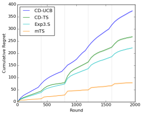
Figure 2: Mean and standard error of regret across $100$ runs with fixed change-points.

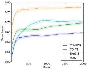
(a) Random latent states, fixed model.

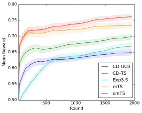
(b) Random latent states, uncertain model.

Figure 3: Mean and standard error of reward across $100$ runs in synthetic scenarios.

5.1 Synthetic Experiments

We artificially create a non-stationary multi-armed bandit without context, with $\mathcal{A}=[5]$ and $\mathcal{S}=[5]$. Mean rewards for are sampled uniformly at random $\mu(a,s)\sim\mathsf{Uniform}(0,1)$ for each $a\in\mathcal{A},s\in\mathcal{S}$. Rewards are drawn i.i.d. from $P(\cdot\mid a,s)=\mathcal{N}(\cdot\mid\mu(a,s),\sigma^{2})$ with $\sigma=0.5$. We use a horizon of $n=2000$ as a primary application we are concerned with is fast personalization.

For $\tt CD\mathchar 45\relax UCB$, $\tt CD\mathchar 45\relax TS$, we use a change-point detector that computes the sum of the rewards for each arm in the past $\tau/2$ rounds, and the $\tau/2$ rounds before that. If the absolute value of their difference is greater than a threshold $b$, a change is detected. Following Cao et al. (2019), the window length parameter was tuned to $\tau=100$ to minimize regret, and the threshold is chosen to be $b=\sigma\sqrt{\tau\log(2|\mathcal{A}|n^{2})/2}$.

First, we consider the specific setting where fixed changes between latent states occur exactly every $200$ rounds. We give model-based algorithms $\tt Exp3.S$ and $\tt mTS$ the true mean rewards. In Figure 3, we report the cumulative regret of all methods across $100$ runs. Because we use a short horizon, baseline bandit algorithms that are more sample inefficient and drastically outperformed by our method which leverages a prior model. Next, we assume random latent state changes according to a transition matrix with $0.0025$ probability of uniformly changing to another latent state, meaning the latent state changes every $200$ rounds in expectation. In Figure 3, we show the mean reward of each method across $100$ independent runs under two different scenarios: (i) the reward model and transition matrix are known; (ii) mean rewards are drawn from a Gaussian prior $\mathcal{N}(\mu(a,s),\sigma_{0}^{2})$ with $\sigma_{0}=0.2$, and transitions are drawn from a Dirichlet prior with $0.005$ expected probability of transition, i.e. for a state $s$, $\phi_{s}\sim\mathsf{Dir}((\alpha_{s,s^{\prime}})_{s^{\prime}\in\mathcal{S}})$ where parameters $(\alpha_{s})_{s\in\mathcal{S}}$ satisfy $\alpha_{s,s^{\prime}}=796$ if $s^{\prime}=s$ and $1$ otherwise.

When a prior is given, $\tt mTS$ uses the mean of the prior as if it were the true model parameter, resulting in a performance gap due to model misspecification. We report the average reward in Figure 3 because the regret becomes dominated by model error in the given offline model. In all cases, the model-based Thompson sampling algorithms outperform all baselines by a significant margin, and do not require extensive hyperparameter tuning as the baselines did. Also, as uncertainty is introduced in the offline model, $\tt mTS$ performs worse than $\tt umTS$, which accounts for model uncertainty.

5.2 MovieLens Experiments

We also assess the performance of our algorithms on the MovieLens 1M dataset (Harper and Konstan, 2015), a popular collaborative filtering dataset, where $6040$ users rate $3883$ movies. Each movie has a set of genres. We filter the dataset to include only users who rated at least $200$ movies and movies rated by at least $200$ users. This results in $1353$ users and $1124$ movies. We randomly select $50\%$ of all ratings as our offline training set, and use the remaining $50\%$ as a test set, giving sparse ratings matrices $M_{\text{train}}$ and $M_{\text{test}}$. We complete each matrix using least-squares matrix completion (Salakhutdinov and Mnih, 2008) with rank $20$ to yield a low prediction error without overfitting. The learned training (test) factors are $M_{\text{train}}=\widehat{U}\widehat{V}^{\top}$ ($M_{\text{test}}=UV^{\top}$). In the training (test) set, user $i$ and movie $j$ correspond to the rows in the corresponding matrix, $\widehat{U}_{i}$ ($U_{i}$) and $\widehat{V}_{i}$ ($V_{j}$).

We define a non-stationary latent contextual bandit instance with $\mathcal{A}=[20]$ and $\mathcal{S}=[5]$ as follows. We use $k$-means clustering on the rows of $U$ to cluster users into $5$ clusters, where $5$ is the largest value that yields evenly-sized clusters. Motivated by prior work (Wu et al., 2018), we create a superuser by randomly sampling $5$ users $i_{1},\dots,i_{5}$, one from each cluster; for latent state $s$, the superuser behaves according to the user $i_{s}$. Note that different superusers will have a different set of behavior modes, which is often true in practice. The transition matrix that governs the dynamics of the superuser is given by the linear combination $P(s^{\prime}\mid s;\phi_{*})=0.9J(s,s^{\prime})+0.1K(s,s^{\prime}),$ where $J(s,s^{\prime})=1-p$ if $s^{\prime}=s$ and $p/(|\mathcal{S}|-1)$ otherwise, and $K(s,s^{\prime})\propto\exp(||U_{i_{s^{\prime}}}-U_{i_{s}}||_{2}^{2})$. Here $J$ is used to ensure changes are infrequent, and $K$ to make transitions to similar latent states more likely. We let $p=0.9975$ so that changes occur roughly every $400$ rounds with $n=2000$.

A run of a non-stationary contextual bandit proceeds as follows. A superuser $i_{1},\ldots,i_{5}$ is sampled at random as described above. In each round, a latent state $S_{t}$ is generated according to $S_{t-1}$ and the transition matrix. Then, $20$ genres, then a movie for each genre, are both uniformly sampled from the set of all genres, movies, respectively, creating a set of diverse movies. Context $X_{t}\in\mathbb{R}^{20\times 20}$ is a matrix where the rows are the training feature vectors of the sampled movies, that is movie $j$ has a vector $\widehat{V}_{j}$. The agent chooses among movies in $X_{t}$. The reward for recommending movie $j$ to the superuser under state $S_{t}=s$ is drawn from $R_{t}\sim\mathcal{N}(U_{i_{s}}^{\top}V_{j},0.25)$, the product of the test user and movie vectors as its mean. Note that both $U$ and $V$ are unknown to the learning agent.

Our baselines $\tt CD\mathchar 45\relax LinUCB$, $\tt CD\mathchar 45\relax LinTS$ are given movie vectors from the training set as context, and need to only learn the user vector. We could not find prior work that performed change detection in linear bandits, so we propose an adaption of the one by Cao et al. (2019) to the linear case. Specifically, for round $t$ and window size $\tau$, the detector computes the least-squares solution $\widehat{W}_{t}$ with features $X_{t,A_{t}}$ and rewards $R_{t}$ for the past $\tau/2$ rounds of data, and $\widehat{W}_{t}^{\prime}$ for the $\tau/2$ rounds before that. Let $\widehat{\Sigma}_{t}=\sum_{t-\tau}^{t}X_{t,A_{t}}^{\top}X_{t,A_{t}}$ be the empirical covariance matrix. The detector fires when $||\widehat{W}_{t}-\widehat{W}_{t}^{\prime}||_{\widehat{\Sigma}_{t}}\geq b$; for matrix $M$ and weights $\Sigma$, the weighted norm is given by $||M||_{\Sigma}=\sqrt{M^{T}\Sigma M}$. Here both $\tau$ and $b$ are tuned $\tau=100$ and $b=13$ by maximizing reward during evaluation.

We learn a model offline in the same way as the true model is constructed, except using the training set. Our offline model consists of $5$ clusters of users derived from $k$-means clustering on users $\widehat{U}$ in the training set. For each latent state, the prior given to our algorithms is a Gaussian prior with the corresponding cluster’s mean and covariance. Similarly, we estimate a transition matrix $\widehat{\phi}$ using the same process as $\phi_{*}$ but using the cluster means on the training set instead of user features on the test set. We give a Dirichlet prior with parameters $(\alpha_{s,s^{\prime}})_{s,s^{\prime}\in\mathcal{S}\times\mathcal{S}}$ where $\alpha_{s,s^{\prime}}=800\,P(s^{\prime}\mid s;\widehat{\phi})$.

We evaluate on $100$ superusers, and show the mean reward in Figure 4. Again, the model-based algorithms outperform finely-tuned baselines by a significant margin, especially in the short horizon. Since the offline model is misspecified due to the train-test split, $\tt umTS$ improves upon $\tt mTS$ in the long term, as it refines its model parameters online.

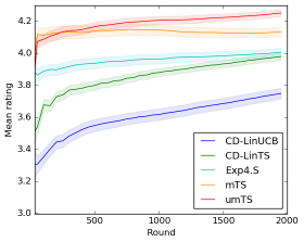
Figure 4: Mean and standard error of reward across 100 “superusers” in MovieLens 1M.

6 Related Work

Non-stationary Bandits.

This topic has been studied extensively (Kocsis and Szepesvari, 2006; Garivier and Moulines, 2008; Auer et al., 2002b). First works adapted to changes passively by weighting rewards, either by exponential discounting (Kocsis and Szepesvari, 2006) or by considering recent rewards in a sliding window (Garivier and Moulines, 2008). The latter yields a $\tilde{\mathcal{O}}(K\sqrt{nL}/\Delta^{2})$ gap-dependent bound when $L$ is known. In the adversarial setting (Auer et al., 2002b; Auer, 2003), adaptation can be achieved by bounding the weights of experts from below. This leads to $\tilde{\mathcal{O}}(\sqrt{n|\mathcal{S}|L})$ gap-free switching regret, where $|\mathcal{S}|$ is the number of experts. Besbes et al. (2014) periodically reset a base bandit algorithm and attain $\tilde{\mathcal{O}}(n^{2/3}V_{T}^{1/3})$ regret, where $V_{T}$ is the total variation under smooth changes. Other works monitor reward distributions and reset the bandit algorithm when a change is detected  (Yu and Mannor, 2009; Liu et al., 2018). Mellor and Shapiro (2013) proposed augmenting Thompson sampling with a Bayesian change-point detector, but provide no regret guarantee. Cao et al. (2019) proposed a simple near-optimal change-point detector that yields $\tilde{\mathcal{O}}(\sqrt{nKL})$ regret. In linear bandits, several recent paper studied passive adaptation of UCB algorithms (Cheung et al., 2019; Russac et al., 2019; Zhao et al., 2020). This yields $\tilde{\mathcal{O}}(n^{2/3}P_{T}^{1/3})$ regret, where $P_{T}$ measures the total variation in an unknown weight vector. Luo et al. (2018) provided several contextual algorithms with similar regret to ours, with the best algorithm matching the Exp4.S bound of $\tilde{\mathcal{O}}(\sqrt{n|\mathcal{S}|L})$. All above methods forget the past, discount it, or are adversarial. This is a major drawback when the environment changes in a structured manner.

Latent Bandits.

Our work is also related to latent bandits (Maillard and Mannor, 2014; Zhou and Brunskill, 2016). Here the latent state is fixed across rounds and algorithms compete with standard bandit strategies, such as UCB  (Auer et al., 2002a; Abbasi-yadkori et al., 2011) or Thompson sampling (Agrawal and Goyal, 2013; Abeille and Lazaric, 2016). Maillard and Mannor (2014) derived UCB algorithms in the multi-armed case without context under the extremes when the mean conditional rewards are either known or need to be estimated completely online. Zhou and Brunskill (2016) extended it to contextual bandits where policies are learned offline and selected online using Exp4. Bayesian policy reuse (BPR) (Rosman et al., 2016) selects offline-learned policies by maintaining a belief over the optimality of each policy, but no regret analysis exists. Recently, Hong et al. (2020) proposed and analyzed TS algorithms with complex offline-learned models. Our work is the first to extend latent bandits to non-stationary environments by considering a latent state that evolves according to a transition model, which is known or sampled from a known prior.

7 Conclusions

We study non-stationary latent bandits, where the conditional rewards depend on an evolving discrete latent state. Given the plethora of rich offline models, we consider a setting where an offline-learned model can be used naturally by Thompson sampling to identify the latent state online. Prior algorithms for non-stationary bandits adapt by forgetting the past, discounting it, or are adversarial. We avoid this by leveraging the stochastic latent structure of our problem and thus can outperform prior works empirically by a large margin. Our approach is contextual, aware of uncertainty, and we analyze it by a reduction to a sliding-window UCB algorithm. Though our analysis is conservative, our work can be viewed as a stepping stone for analyzing the Bayes regret of Thompson sampling in more complex graphical models than a single fixed latent state (Maillard and Mannor, 2014; Zhou and Brunskill, 2016; Hong et al., 2020).

Appendix A Proofs

Our proofs rely on the following concentration inequality, which is a straightforward extension of the Azuma-Hoeffding inequality to sub-Gaussian random variables. This was used and proved by Hong et al. (2020).

Proposition 2.

Let $(Y_{t})_{t\in[n]}$ be a martingale difference sequence with respect to filtration $(\mathcal{F}_{t})_{t\in[n]}$, that is $\mathbb{E}\left[Y_{t}\mid\mathcal{F}_{t-1}\right]=0$ for any $t\in[n]$. Let $Y_{t}\mid\mathcal{F}_{t-1}$ be $\sigma^{2}$-sub-Gaussian for any $t\in[n]$. Then for any $\varepsilon>0$,

$$\mathbb{P}\left(\Big{|}\sum_{t=1}^{n}Y_{t}\Big{|}\geq\varepsilon\right)\leq 2\exp\left[-\frac{\varepsilon^{2}}{2n\sigma^{2}}\right]\,.$$

A.1 Proof of Lemma 1

Recall that we have the following fixed quantities: true reward parameters $\theta_{*}$, latent state sequence $s_{1:n}$, and the number of stationary segments $L$. Note that we can decompose the regret as

$$\begin{split}\mathcal{R}(n;\theta_{*},s_{1:n})&=\mathbb{E}\left[\sum_{t=1}^{n}\left(\mu(A_{t,*},X_{t},s_{t};\theta_{*})-\mu(A_{t},X_{t},s_{t};\theta_{*})\right)\right]\\ &=\mathbb{E}\left[\sum_{t=1}^{n}\left(\mu(A_{t,*},X_{t},s_{t};\theta_{*})-U_{t}(A_{t})\right)\right]+\mathbb{E}\left[\sum_{t=1}^{n}\left(U_{t}(A_{t})-\mu(A_{t},X_{t},S_{t};\theta_{*})\right)\right]\\ &\leq\mathbb{E}\left[\sum_{t=1}^{n}\left(\mu(A_{t,*},X_{t},s_{t};\theta_{*})-U_{t}(A_{t,*})\right)\right]+\mathbb{E}\left[\sum_{t=1}^{n}\left(U_{t}(A_{t})-\mu(A_{t},X_{t},S_{t};\theta_{*})\right)\right]\,.\end{split}$$ (11)

This is because for all rounds $t\in[n]$, we choose $A_{t}=\arg\max_{a\in\mathcal{A}}U_{t}(a)$, which means $U_{t}(A_{t})\geq U_{t}(A_{t,*})$.

Let $\mathcal{T}$ be a set of all rounds $t$ that are not close to any change-point, that is $s_{\ell}=s_{t}$ for all $\ell\in\{t-\tau+1,\ldots,t\}$. Note that this includes all rounds where the last $\tau$ rounds have the same latent state as that round. Let

$$E_{t}=\left\{\forall s\in\mathcal{S}:\,\left|\sum_{\ell=\min\{1,t-\tau\}}^{t-1}\mathbbm{1}\left\{B_{\ell}=s\right\}\left(\mu(A_{\ell},X_{\ell},s_{\ell};\theta_{*})-R_{\ell}\right)\right|\leq\sigma\sqrt{6N_{t}(s)\log n}\right\}$$ (12)

be the event that the total realized reward under each played latent state is close to its expectation. Let $E=\cap_{t\in\mathcal{T}}E_{t}$ be the event that this holds for all rounds not close to a change-point, and $\bar{E}$ be its complement. Then we can bound the expected $n$-round regret as

$$\begin{split}&\mathcal{R}(n;\theta_{*},s_{1:n})\\ &\,\leq L\tau+\mathbb{E}\left[\sum_{t\in\mathcal{T}}\left(\mu(A_{t,*},X_{t},s_{t};\theta_{*})-\mu(A_{t},X_{t},s_{t};\theta_{*})\right)\right]\\ &\,=L\tau+\mathbb{E}\left[\mathbbm{1}\left\{\bar{E}\right\}\sum_{t\in\mathcal{T}}\left(\mu(A_{t,*},X_{t},s_{t};\theta_{*})-\mu(A_{t},X_{t},s_{t};\theta_{*})\right)\right]+\mathbb{E}\left[\mathbbm{1}\left\{E\right\}\sum_{t\in\mathcal{T}}\left(\mu(A_{t,*},X_{t},s_{t};\theta_{*})-\mu(A_{t},X_{t},s_{t};\theta_{*})\right)\right]\\ &\,\leq L\tau+\mathbb{E}\left[\mathbbm{1}\left\{\bar{E}\right\}\sum_{t\in\mathcal{T}}\left(\mu(A_{t,*},X_{t},s_{t};\theta_{*})-\mu(A_{t},X_{t},s_{t};\theta_{*})\right)\right]\\ &\,\qquad+\mathbb{E}\left[\mathbbm{1}\left\{E\right\}\sum_{t\in\mathcal{T}}\left(\mu(A_{t,*},X_{t},s_{t};\theta_{*})-U_{t}(A_{t,*})\right)\right]+\mathbb{E}\left[\mathbbm{1}\left\{E\right\}\sum_{t\in\mathcal{T}}\left(U_{t}(A_{t})-\mu(A_{t},X_{t},s_{t};\theta_{*})\right)\right]\,,\end{split}$$ (13)

where for the first inequality we upper bound the regret in rounds close to change-points by $L\tau$, and in the second we use the regret decomposition in (11). We ignore the rounds within $\tau$ rounds of change-points because the empirical mean reward estimates over the those rounds are biased.

We first show that the probability of $\bar{E}$ occurring is low. Without context, this would follow immediately from Hoeffding’s inequality. Since we have context generated by some random process, we instead turn to martingales.

Proposition 3.

Let $E_{t}$ be defined as in (12) for all rounds $t$, $E=\cap_{t\in\mathcal{T}}E_{t}$, and $\bar{E}$ be its complement. Then $\mathbb{P}\left(\bar{E}\right)\leq 2|\mathcal{S}|n^{-1}$.

Proof.

Because the UCBs depend on which latent states are eliminated, the UCBs depend on the history, and the conditional action given observed context also depends on the history. For each latent state $s$ and round $t$, let $\mathcal{T}_{t,s}$ be the rounds where state $s$ was chosen among the past $\tau$ rounds. For round $\ell\in\mathcal{T}_{t,s}$, let $Y_{\ell}(s)=\mu(A_{\ell},X_{\ell},s_{\ell};\theta_{*})-R_{\ell}$. Observe that $Y_{\ell}(s)\mid X_{\ell},H_{\ell}$ is $\sigma^{2}$-sub-Gaussian. This implies that $(Y_{\ell}(s))_{\ell\in\mathcal{T}_{t,s}}$ is a martingale difference sequence with respect to context and history $(X_{\ell},H_{\ell})_{\ell\in\mathcal{T}_{t,s}}$, or $\mathbb{E}\left[Y_{\ell}(s)\mid X_{\ell},H_{\ell}\right]=0$ for all rounds $\ell\in\mathcal{T}_{t,s}$.

For any round $t$, and state $s\in\mathcal{S}$, we have that $\mathcal{T}_{t,s}$ is a random quantity. First, we fix $|\mathcal{T}_{t,s}|=N_{t}(s)=u$ where $u\leq\tau$ and yield the following due to Proposition 2,

$$\mathbb{P}\left(\left|\sum_{\ell\in\mathcal{T}_{t,s}}Y_{\ell}(s)\right|\geq\sigma\sqrt{6u\log n}\right)\leq 2\exp\left[-3\log n\right]=2n^{-3}\,.$$

So, by the union bound, we have

$$\mathbb{P}\left(\bar{E}\right)\leq\sum_{t\in\mathcal{T}}\sum_{s\in\mathcal{S}}\sum_{u=1}^{\tau}\mathbb{P}\left(\left|\sum_{\ell\in\mathcal{T}_{t,s}}Y_{\ell}(s)\right|\geq\sigma\sqrt{6u\log n}\right)\leq 2|\mathcal{S}|n^{-1}\,.$$

This concludes the proof. ∎

We can show that the second term in (LABEL:eqn:sw_regret_event_decomposition) is small because the probability of $\bar{E}$ is small. Specifically, from Proposition 3, and that total regret is bounded by $n$, we have that the second term in (LABEL:eqn:sw_regret_event_decomposition) is bounded by $n\mathbb{P}\left(\bar{E}\right)\leq 2|\mathcal{S}|$.

Next, we bound the third term in (LABEL:eqn:sw_regret_event_decomposition). For round $t\in\mathcal{T}$, the event $\mu(A_{t,*},X_{t},s_{t};\theta_{*})>U_{t}(A_{t,*})$ occurs only if $s_{t}\notin C_{t}$ also occurs. By the design of $C_{t}$ in $\tt SW\mathchar 45\relax mUCB$, this happens only if $G_{t}(s_{t})>\sigma\sqrt{6N_{t}(s)\log n}$. Event $E_{t}$ says that the opposite is true for all states, including true state $s_{t}$. So the third term in (LABEL:eqn:sw_regret_event_decomposition) is at most $0$.

Now we consider the last term in (LABEL:eqn:sw_regret_event_decomposition). We know that $\mathcal{T}$ is composed of $L$ stationary segments. We bound the last term for each segment individually as follows.

Proposition 4.

Let $\mathcal{I}\subseteq\mathcal{T}$ be a stationary segment containing $m$ rounds. Then

$$\mathbb{E}\left[\mathbbm{1}\left\{E\right\}\sum_{t\in\mathcal{I}}\left(U_{t}(A_{t})-\mu(A_{t},X_{t},s_{t};\theta_{*})\right)\right]\leq|\mathcal{S}|\lceil m/\tau\rceil+2\sigma\sqrt{6|\mathcal{S}|\lceil m/\tau\rceil m\log{n}}.$$

Proof.

To ease exposition, let the $m$ rounds in $\mathcal{I}$ be denoted $1,\ldots,m$. We can further divide $\mathcal{I}$ into intervals of length $\tau$ and the last with length of at most $\tau$. Let $1=t_{0}\leq t_{1}\leq\ldots\leq t_{\lceil m/\tau\rceil}=m$ partition $\mathcal{I}$ into such intervals. We can write,

$$\mathbb{E}\left[\mathbbm{1}\left\{E\right\}\sum_{t\in\mathcal{I}}\left(U_{t}(A_{t})-\mu(A_{t},X_{t},s_{t};\theta_{*})\right)\right]$$

$$\quad=\mathbb{E}\left[\mathbbm{1}\left\{E\right\}\sum_{i=1}^{\lceil m/\tau\rceil}\sum_{\ell=t_{i-1}}^{t_{i}}\left(\mu(A_{\ell},X_{\ell},B_{\ell};\theta_{*})-R_{\ell}\right)\right]+\mathbb{E}\left[\mathbbm{1}\left\{E\right\}\sum_{i=1}^{\lceil m/\tau\rceil}\sum_{\ell=t_{i-1}}^{t_{i}}\left(R_{\ell}-\mu(A_{\ell},X_{\ell},s_{\ell};\theta_{*})\right)\right]$$

$$\quad\leq\mathbb{E}\left[\sum_{i=1}^{\lceil m/\tau\rceil}\sum_{s\in S}(G_{t_{i}}(s)+1)\right]+\sum_{i=1}^{\lceil m/\tau\rceil}\sum_{s\in S}\sigma\sqrt{6N_{t_{i}}(s)\log n}$$

$$\quad\leq|\mathcal{S}|\lceil m/\tau\rceil+\sum_{s\in S}\sum_{i=1}^{\lceil m/\tau\rceil}2\sigma\sqrt{6N_{t_{i}}(s)\log n}.$$

For each window $i$ of length $\tau$ and latent state $s$, we use that until the last round before $t_{i}$ where $s$ is selected, we have an upper bound on the total prediction error, given by the upper bound on the gap $G_{t_{i}}(s)\leq\sigma\sqrt{6N_{t_{i}}(s)\log n}$, where $G_{t_{i}}(s)$ is defined as in (10) Recall that $E_{t_{i}}$, as defined in (12), occurring implies that the deviation of the realized reward from the true means bounded by $\sigma\sqrt{6N_{t_{i}}(s)\log n}$. Accounting for the last round where $s$ was chosen in window $i$ yields the right-hand side of the inequality. Applying the Cauchy-Schwarz inequality yields,

$$\mathbb{E}\left[\mathbbm{1}\left\{E\right\}\sum_{t\in\mathcal{I}}U_{t}(A_{t})-\mu(A_{t},X_{t},s_{t};\theta_{*})\right]\leq|\mathcal{S}|\lceil m/\tau\rceil+2\sigma\sqrt{6|\mathcal{S}|\lceil m/\tau\rceil m\log{n}},$$

which is the desired upper bound. ∎

Now we can bound the last term in (LABEL:eqn:sw_regret_event_decomposition) by combining Proposition 4 across all $L$ stationary segments. Let $(\mathcal{I}_{i})_{i\in[L]}$ denote the stationary segments, and segment $\mathcal{I}_{i}$ have length $m_{i}$. We have,

$$\mathbb{E}\left[\mathbbm{1}\left\{E\right\}\sum_{t\in\mathcal{T}}\left(U_{t}(A_{t})-\mu(A_{t},X_{t},s_{t};\theta_{*})\right)\right] =\mathbb{E}\left[\mathbbm{1}\left\{E\right\}\sum_{i=1}^{L}\sum_{t\in\mathcal{I}_{i}}\left(U_{t}(A_{t})-\mu(A_{t},X_{t},s_{t};\theta_{*})\right)\right]$$

$$\leq\sum_{i=1}^{L}|\mathcal{S}|\lceil m_{i}/\tau\rceil+2\sigma\sqrt{6|\mathcal{S}|\lceil m_{i}/\tau\rceil m_{i}\log{n}}$$

$$\leq|\mathcal{S}|(n/\tau)+2\sigma\sqrt{6|\mathcal{S}|(n/\tau)n\log{n}}.$$

Here we use that for any segment $i$, we have $\lceil m_{i}/\tau\rceil\leq(m_{i}+\tau)/\tau$ for any number of rounds $m$, and that $\sum_{i}m_{i}=n-L\tau$ because we omitted rounds to close to a change-point. Combining the bounds for all terms in (LABEL:eqn:sw_regret_event_decomposition) yields,

$$\mathcal{R}(n;\theta_{*},s_{1:n}) \leq L\tau+2|\mathcal{S}|+|\mathcal{S}|(n/\tau)+2\sigma\sqrt{6|\mathcal{S}|(n/\tau)n\log n},$$

When $L$ is known, we can solve for the optimal window length $\tau=\mathcal{O}(n^{2/3}\sqrt{|\mathcal{S}|\log n/L})$, which when substituted into the regret bound yields $\mathcal{R}(n;\theta_{*},s_{1:n})=\mathcal{O}(n^{2/3}\sqrt{|\mathcal{S}|L\log n})$ , as desired.

A.2 Proof of Theorem 1

From the Bayes regret formulation in (2), the true latent state sequence $S_{1:n}\in\mathcal{S}^{n}$ is random for a fixed transition model $\phi_{*}$. Here we still assume a fixed reward model $\theta_{*}$. We have that the optimal action $A_{t,*}=\arg\max_{a\in\mathcal{A}}\mu(a,X_{t},S_{t};\theta_{*})$ is random not only due to context, but also latent state $S_{t}$. We also have that $L=\sum_{t=1}^{n}\mathbbm{1}\left\{S_{t}\neq S_{t-1}\right\}$ is random due to latent state sequence $S_{1:n}$.

Similar to Russo and Van Roy (2013), we reduce our analysis of $\tt mTS$ to analysis of $\tt SW\mathchar 45\relax mUCB$ as done in Lemma 1. We define $U_{t}(a)=\arg\max_{s\in C_{t}}\mu(a,X_{t},s;\theta_{*})$ where the $C_{t}$ is as in $\tt SW\mathchar 45\relax mUCB$. Recall that the Bayes regret is given by (2), and can be decomposed as (9). In Section A.1, we bounded an equivalent regret decomposition for any $\theta_{*},S_{1:n}$ and therefore also in expectation over $S_{1:n}\sim\phi_{*}$. We have the Bayes regret bound,

$$\mathcal{BR}(n;\theta_{*},\phi_{*}) =\mathbb{E}\left[\sum_{t=1}^{n}\left(\mu(A_{t,*},X_{t},S_{t};\theta_{*})-U_{t}(A_{t,*})\right)\mid\theta_{*},\phi_{*}\right]+\mathbb{E}\left[\sum_{t=1}^{n}\left(U_{t}(A_{t})-\mu(A_{t},X_{t},S_{t};\theta_{*})\right)\mid\theta_{*},\phi_{*}\right]$$

$$\leq\mathbb{E}_{S_{1:n}\sim\phi_{*}}\left[L\tau+2|\mathcal{S}|+|\mathcal{S}|(n/\tau)+2\sigma\sqrt{6|\mathcal{S}|(n/\tau)n\log n}\right],$$

where we directly substitute the upper bound in Lemma 1 inside the expectation.

Since $\phi_{*}$ is known, we can define $p=1-\min_{s\in\mathcal{S}}P(s\mid s;\phi_{*})$ as the maximum probability of a change occurring. Then number of change-points $L-1$ is a binomial random variable, so that $\mathbb{E}_{S_{1:n}\sim\phi_{*}}\left[L\right]=1+pn=\tilde{L}$. For optimal choice of $\tau=\mathcal{O}(n^{2/3}\sqrt{|\mathcal{S}|\log n/L})$, we can simplify the expectation over random $L$ to yield,

$$\mathcal{BR}(n;\theta_{*},\phi_{*})=\mathcal{O}\left(n^{2/3}\sqrt{|\mathcal{S}|\mathbb{E}_{S_{1:n}\sim\phi_{*}}\left[L\right]\log n}\right)=\mathcal{O}\left(n^{2/3}\sqrt{|\mathcal{S}|\tilde{L}\log n}\right),$$

where we use Jensen’s inequality and that the expression inside the expectation is concave in $L$.

A.3 Proof of Theorem 2

From the Bayes regret formulation in (3), both the reward and transition model parameters $\theta_{*},\phi_{*}$ are now random according to priors $P_{1}(\theta),P_{1}(\phi)$, respectively. We have that the optimal action $A_{t,*}=\arg\max_{a\in\mathcal{A}}\mu(a,X_{t},S_{t};\theta_{*})$ is random due to context $X_{t}$, latent state $S_{t}$, and model $\theta_{*}$.

Recall that given prior $P_{1}(\theta)$, we have that $\bar{\mu}(a,x,s)=\int_{\theta}\mu(a,x,s;\theta)P_{1}(\theta)d\theta$ is the mean conditional reward marginalized with respect to the prior. We make one small change to (10) in $\tt SW\mathchar 45\relax mUCB$, which accounts for uncertainty: for round $t$ and state $s$, instead of acting according to true means $\mu(A_{t},X_{t},s;\theta_{*})$, we act conservatively according to the mean marginalized over the prior $\bar{\mu}(A_{t},X_{t},s)$. Formally, the gap in $\tt SW\mathchar 45\relax umUCB$ is redefined as

$$G_{t}(s)=\sum_{\ell=\max\{1,t-\tau\}}^{t-1}\mathbbm{1}\left\{B_{\ell}=s\right\}\left(\bar{\mu}(A_{\ell},X_{\ell},s)-\varepsilon-R_{\ell}\right).$$ (14)

The additional $\varepsilon$ ensures that we do not mistakenly eliminate the true latent state from $C_{t}$ due to a prediction error.

Our proof uses the following regret bound for $\tt SW\mathchar 45\relax umUCB$, which is for a fixed $\theta_{*}$ sampled from the prior.

Lemma 2.

For fixed model parameters $\theta_{*}$, assume that there exist $\varepsilon>0$ such that $\theta_{*}$ satisfies the following: $\left\{\forall a\in\mathcal{A},x\in\mathcal{X},s\in\mathcal{S}:|\bar{\mu}(a,x,s)-\mu(a,x,s;\theta_{*})|\leq\varepsilon\right\}.$ Then for optimal $\tau$, the $n$-round regret of $\tt SW\mathchar 45\relax umUCB$ is

$$\mathcal{R}(n;\theta_{*},s_{1:n}) =\mathcal{O}\left(\varepsilon n+n^{2/3}\sqrt{|\mathcal{S}|L\log n}\right).$$

Proof.

We have the same regret decomposition for $n$-round regret, stated in (LABEL:eqn:sw_regret_event_decomposition). The analysis proceeds similarly to Section A.1, only we need to additionally account for prediction error in the conditional mean rewards. We only highlight the differences, and defer other details of the proof to Section A.1.

Using Proposition 3, and that the total regret is bounded by $n$, we again have the second term in (LABEL:eqn:sw_regret_event_decomposition) can be bounded by, $n\mathbb{P}\left(\bar{E}\right)\leq 2|\mathcal{S}|$. Bounding the third term in (LABEL:eqn:sw_regret_event_decomposition) requires a slight change. For round $t\in\mathcal{T}$, we have that the event $\mu(A_{t,*},X_{t},s_{t};\theta_{*})-U_{t}(A_{t,*})>\varepsilon$ occurs only if $s_{t}\notin C_{t}$. By the design of $C_{t}$ in $\tt SW\mathchar 45\relax umUCB$, this happens only if $G_{t}(s_{t})>\sigma\sqrt{6N_{t}(s)\log n}$, since

$$G_{t}(s_{t})=\smashoperator[r]{\sum_{\ell=\max\{1,t-\tau\}}^{t-1}}\mathbbm{1}\left\{B_{\ell}=s_{t}\right\}\left(\bar{\mu}(A_{\ell},X_{\ell},s_{t})-\varepsilon-R_{\ell}\right)\leq\smashoperator[r]{\sum_{\ell=\max\{1,t-\tau\}}^{t-1}}\mathbbm{1}\left\{B_{\ell}=s_{*}\right\}\left(\mu(A_{\ell},X_{\ell},s_{t};\theta_{*})-R_{\ell}\right).$$

Event $E_{t}$ says that the opposite is true for all states, including true state $s_{t}$. So the third term in (LABEL:eqn:sw_regret_event_decomposition) is at most $\varepsilon n$.

For the last term in (LABEL:eqn:sw_regret_event_decomposition), we need to account for the fact that $\varepsilon$ is included in the gap $G_{t}(s)$ for every round $t$ and state $s$. To do so, we introduce a $\varepsilon n$ term in the expression as,

$$\mathbb{E}\left[\mathbbm{1}\left\{E\right\}\sum_{t\in\mathcal{T}}\left(U_{t}(A_{t})-\mu(A_{t},X_{t},s_{t};\theta_{*}\right)\right]\leq\varepsilon n+\mathbb{E}\left[\mathbbm{1}\left\{E\right\}\sum_{t\in\mathcal{T}}\left(U_{t}(A_{t})-\varepsilon+\mu(A_{t},X_{t},s_{t};\theta_{*})\right)\right]$$

The second term on the right-hand side can be bounded the same way as in Section A.1 by introducing the realized reward, and bounding the sum of confidence widths using the gap given in (14).

This yields the bound on total regret,

$$\mathcal{R}(n;\theta_{*},s_{1:n}) \leq L\tau+2\varepsilon n+|\mathcal{S}|(n/\tau+2)+2\sigma\sqrt{6|\mathcal{S}|(n/\tau)n\log n}.$$

Solving for optimal window length in terms of $L$ yields $\tau=\mathcal{O}(n^{2/3}\sqrt{|\mathcal{S}|\log n/L})$, which when substituted into the regret gives $\mathcal{R}(n;\theta_{*},s_{1:n})=\mathcal{O}(\varepsilon n+n^{2/3}\sqrt{|\mathcal{S}|L\log n})$ , as desired. ∎

In order to prove Theorem 2, we again reduce to the proof of Lemma 2 for $\tt SW\mathchar 45\relax umUCB$. We define $U_{t}(a)=\arg\max_{s\in C_{t}}\mu(a,X_{t},s;\theta_{*})$ as in $\tt SW\mathchar 45\relax umUCB$. We also define event

$$\mathcal{E}=\{\forall a\in\mathcal{A},x\in\mathcal{X},s\in\mathcal{S}:\left|\bar{\mu}(a,x,s)-\mu(a,x,s;\theta_{*})\right|\leq\varepsilon\},$$

for when the sampled true model $\theta_{*}$ behaves close to expected, and $\bar{\mathcal{E}}$ as its complement. If $\mathcal{E}$ does not hold, then the best possible upper bound on regret is $n$; fortunately, we assume in the statement of the theorem that the probability of that occurring is bounded by $\delta$. So we can bound the $n$-round Bayes regret as

$$\mathcal{BR}(n)=\mathbb{E}\left[\mathbbm{1}\left\{\bar{\mathcal{E}}\right\}\mathcal{R}(n,\theta_{*},s_{1:n})\right]+\mathbb{E}\left[\mathbbm{1}\left\{\mathcal{E}\right\}\mathcal{R}(n;\theta_{*},s_{1:n})\right]\leq\delta n+\mathbb{E}\left[\mathbbm{1}\left\{\mathcal{E}\right\}\mathcal{R}(n;\theta_{*},s_{1:n})\right].$$

The second term can be decomposed as in (9) and bounded by Lemma 2 as the bound in the lemma is worst-case over any model parameters $\theta_{*}$ and sequence $S_{1:n}$. We have the Bayes regret bound,

$$\mathcal{BR}(n) \leq\delta n+2\varepsilon n+\mathbb{E}_{\phi_{*}\sim P_{1}}\left[L\tau+2|\mathcal{S}|+|\mathcal{S}|(n/\tau)+2\sigma\sqrt{6|\mathcal{S}|(n/\tau)n\log n}\right].$$

Here $\phi_{*}$ is random, and hence number of stationary segments $L$ is also random. Let $p$ denote the maximum probability of change, i.e., for fixed $\phi_{*}$, we have $p=1-\min_{s\in\mathcal{S}}P(s\mid s;\phi_{*})$ as in Theorem 1. Unlike in Theorem 1, we have that $p$ is random as well due to randomness in $\phi_{*}$. Recall from the statement of Theorem 2 that $(\alpha_{s,s^{\prime}})_{s,s^{\prime}\in\mathcal{S}\times\mathcal{S}}$ are the prior parameters of $P_{1}(\phi)$. We can write $\mathbb{E}_{\phi_{*}\sim P_{1}}\left[p\right]\leq 1-\min_{s\in\mathcal{S}}\alpha_{s,s}/\sum_{s^{\prime}\in\mathcal{S}}\alpha_{s,s^{\prime}}=\tilde{p}.$ This means we can bound the expected value of $L$ as,

$$\mathbb{E}_{\phi_{*}\sim P_{1}}\left[L\right]=\mathbb{E}_{\phi_{*}\sim P_{1}}\left[\mathbb{E}_{S_{1:n}\sim\phi_{*}}\left[L\mid\phi_{*}\right]\right]\leq\mathbb{E}_{\phi_{*}\sim P_{1}}\left[1+pn\right]\leq 1+\tilde{p}n=\tilde{L}.$$

Since the Bayes regret is still concave in $L$, we can apply the same trick as in Section A.2 using Jensen’s inequality, and yield, for optimal choice of $\tau=\mathcal{O}(n^{2/3}\sqrt{|\mathcal{S}|\log n/L})$, the desired Bayes regret bound

$$\mathcal{BR}(n)=\mathcal{O}\left(\delta n+\varepsilon n+n^{2/3}\sqrt{|\mathcal{S}|\mathbb{E}_{\phi_{*}\sim P_{1}}\left[L\right]\log n}\right)=\mathcal{O}\left(\delta n+\varepsilon n+n^{2/3}\sqrt{|\mathcal{S}|\tilde{L}\log n}\right).$$

References

- Abbasi-yadkori et al. (2011) Yasin Abbasi-yadkori, Dávid Pál, and Csaba Szepesvári. Improved algorithms for linear stochastic bandits. In Neural Information Processing Systems, 2011.
- Abeille and Lazaric (2016) Marc Abeille and Alessandro Lazaric. Linear thompson sampling revisited. In Electronic Journal of Statistics, 2016.
- Agrawal and Goyal (2013) Shipra Agrawal and Navin Goyal. Thompson sampling for contextual bandits with linear payoffs. In International Conference on Machine Learning, 2013.
- Anandkumar et al. (2014) Anima Anandkumar, Rong Ge, Daniel J. Hsu, Sham M. Kakade, and Matus Telgarsky. Tensor decompositions for learning latent variable models. In Journal of Machine Learning Research, 2014.
- Auer (2002) Peter Auer. Finite-time analysis of the multiarmed bandit problem. In Machine Learning, 2002.
- Auer (2003) Peter Auer. Using confidence bounds for exploitation-exploration trade-offs. In Journal of Machine Learning Research, 2003.
- Auer et al. (2002a) Peter Auer, Nicolò Cesa-Bianchi, and Paul Fischer. Finite-time analysis of the multiarmed bandit problem. Machine Learning, 2002a.
- Auer et al. (2002b) Peter Auer, Nicolò Cesa-Bianchi, Yoav Freund, and Robert E Schapire. The nonstochastic multiarmed bandit problem. In SIAM journal on computing, 2002b.
- Besbes et al. (2014) Omar Besbes, Yonatan Gur, and Assaf Zeevi. Stochastic multi-armed-bandit problem with non-stationary rewards. In Advances in Neural Information Processing Systems, 2014.
- Cao et al. (2019) Yang Cao, Zheng Wen, Branislav Kveton, and Yao Xie. Nearly optimal adaptive procedure with change detection for piecewise-stationary bandit. In International Conference on Artificial Intelligence and Statistics, 2019.
- Chapelle and Li (2012) Olivier Chapelle and Lihong Li. An empirical evaluation of Thompson sampling. In Neural Information Processing Systems, pages 2249–2257, 2012.
- Cheung et al. (2019) Wang Chi Cheung, David Simchi-Levi, and Ruihao Zhu. Learning to optimize under non-stationarity. In International Conference on Artificial Intelligence and Statistics, 2019.
- Clyde and George (2004) Merlise Clyde and Edward I. George. Model uncertainty. Statistical Science, 2004.
- Doucet et al. (2013) Arnaud Doucet, Neil Gordon, and Nando de Freitas. Sequential Monte Carlo Methods in Practice. Springer New York, 2013.
- Garivier and Moulines (2008) Aurélien Garivier and Eric Moulines. On upper-confidence bound policies for non-stationary bandit problems. In International Conference on Algorithmic Learning Theory, 2008.
- Harper and Konstan (2015) F. Maxwell Harper and Joseph A. Konstan. The MovieLens datasets: History and context. In ACM Transactions on Interactive Intelligent Systems (TiiS), 2015.
- Hartland et al. (2007) Cédric Hartland, Nicolas Baskiotis, Sylvain Gelly, Michèle Sebag, and Olivier Teytaud. Change point detection and meta-bandits for online learning in dynamic environments. 2007.
- Hong et al. (2020) Joey Hong, Branislav Kveton, Manzil Zaheer, Yinlam Chow, Amr Ahmed, and Craig Boutilier. Latent bandits revisited. CoRR, abs/2006.08714, 2020.
- Kocsis and Szepesvari (2006) Levente Kocsis and Csaba Szepesvari. Discounted ucb. In 2nd PASCAL Challenges Workshop, 2006.
- Lai and Robbins (1985) T.L Lai and Herbert Robbins. Asymptotically efficient adaptive allocation rules. In Advances in applied mathematics, 1985.
- Lattimore and Szepesvári (2019) Tor Lattimore and Csaba Szepesvári. Bandit Algorithms. Cambridge University Press, 2019. doi: 10.1017/9781108571401.
- Liu et al. (2018) Fang Liu, Joohyun Lee, and Ness B. Shroff. A change-detection based framework for piecewise-stationary multi-armed bandit problem. In AAAI Conference on Artificial Intelligence, 2018.
- Luo et al. (2018) Haipeng Luo, Chen-Yu Wei, Alekh Agarwal, and John Langford. Efficient contextual bandits in non-stationary worlds. In Conference on Learning Theory, 2018.
- Maillard and Mannor (2014) Odalric-Ambrym Maillard and Shie Mannor. Latent bandits. In International Conference on Machine Learning, 2014.
- Mellor and Shapiro (2013) Joseph Mellor and Jonathan Shapiro. Thompson sampling in switching environments with bayesian online change detection. In International Conference on Artificial Intelligence and Statistics, 2013.
- Rosman et al. (2016) Benjamin Rosman, Majd Hawasly, and Subramanian Ramamoorthy. Bayesian policy reuse. In Machine Learning, 2016.
- Russac et al. (2019) Yoan Russac, Claire Vernade, and Olivier Cappé. Weighted linear bandits for non-stationary environments. In Neural Information Processing Systems, 2019.
- Russo and Van Roy (2013) Daniel Russo and Benjamin Van Roy. Learning to optimize via posterior sampling. CoRR, abs/1301.2609, 2013.
- Salakhutdinov and Mnih (2008) Ruslan Salakhutdinov and Andriy Mnih. Probabilistic matrix factorization. Neural Information Processing Systems, 2008.
- Särkkä (2013) Simo Särkkä. Bayesian Filtering and Smoothing. Cambridge University Press, 2013.
- Thompson (1933) William R. Thompson. On the likelihood that one unknown probability exceeds another in view of the evidence of two samples. Biometrika, 25(3-4):285–294, 1933.
- Wu et al. (2018) Qingyun Wu, Naveen Iyer, and Hongning Wang. Learning contextual bandits in a non-stationary environment. In ACM SIGIR Conference on Research and Development in Information Retrieval, 2018.
- Yu and Mannor (2009) Jia Yuan Yu and Shie Mannor. Piecewise-stationary bandit problems with side observations. In International Conference on Machine Learning, 2009.
- Zhao et al. (2020) Peng Zhao, Lijun Zhang, Yuan Jiang, and Zhi-Hua Zhou. A simple approach for non-stationary linear bandits. In International Conference on Artificial Intelligence and Statistics, 2020.
- Zhou and Brunskill (2016) Li Zhou and Emma Brunskill. Latent contextual bandits and their application to personalized recommendations for new users. In International Joint Conferences on Artificial Intelligence, 2016.