Dual Pixel Exploration: Simultaneous Depth Estimation and Image Restoration
Abstract
The dual-pixel (DP) hardware works by splitting each pixel in half and creating an image pair in a single snapshot. Several works estimate depth/inverse depth by treating the DP pair as a stereo pair. However, dual-pixel disparity only occurs in image regions with the defocus blur. The heavy defocus blur in DP pairs affects the performance of matching-based depth estimation approaches. Instead of removing the blur effect blindly, we study the formation of the DP pair which links the blur and the depth information. In this paper, we propose a mathematical DP model which can benefit depth estimation by the blur. These explorations motivate us to propose an end-to-end DDDNet (DP-based Depth and Deblur Network) to jointly estimate the depth and restore the image. Moreover, we define a reblur loss, which reflects the relationship of the DP image formation process with depth information, to regularise our depth estimate in training. To meet the requirement of a large amount of data for learning, we propose the first DP image simulator which allows us to create datasets with DP pairs from any existing RGBD dataset. As a side contribution, we collect a real dataset for further research. Extensive experimental evaluation on both synthetic and real datasets shows that our approach achieves competitive performance compared to state-of-the-art approaches.
1 Introduction
|
 |
 |
|---|---|---|
|
 |
 |
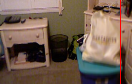
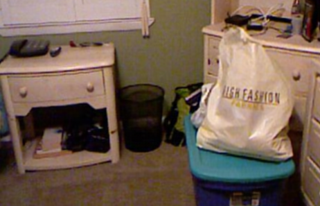
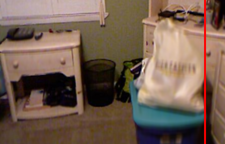
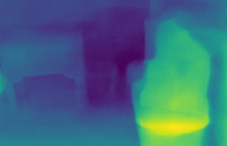
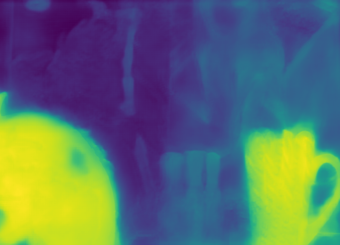
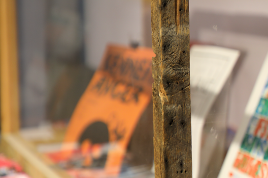
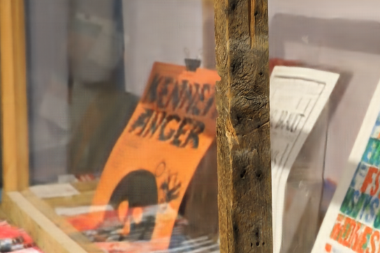
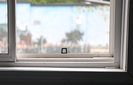
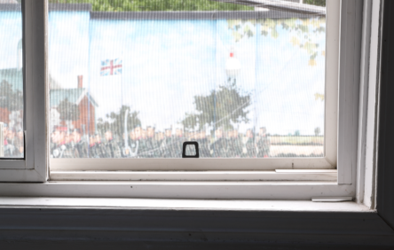
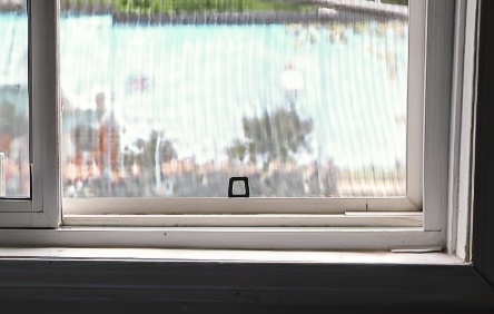
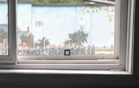
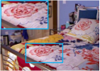
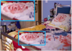
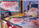
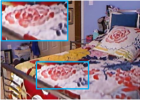
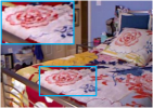
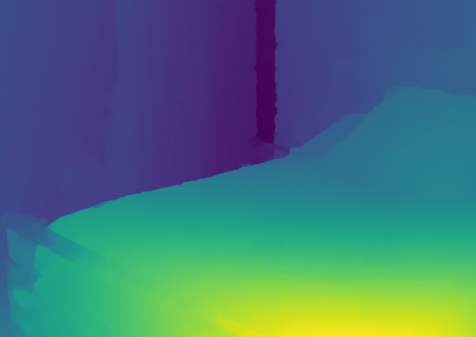
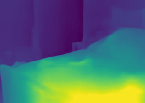
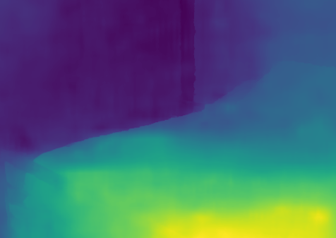
| (a) Inputs | (b) Ours | (c) GT |
The Dual-Pixel (DP) sensor has been used by DSLR (digital single-lens reflex camera) and smartphone cameras to aid focusing. Though the DP sensor is designed for auto-focus [27, 14, 13], it is used in applications such as, depth estimation [9, 24, 38], defocus deblurring [1], reflection removal [25], and shallow Depth-of-Field (DoF) images synthesis [31]. In this paper, we model the imaging process of the DP sensor theoretically, and show its effectiveness for simultaneous depth estimation and image deblurring.
A DP camera simultaneously captures two images, one formed from light rays passing through the right half of the aperture, and one from those passing through the left half of the aperture. Because of the displacement of these two half-apertures, the two images form a stereo pair. The primary role of DP cameras is to enable auto-focus. The set of points in the world that are exactly in focus forms a plane parallel to the lens (perpendicular to the axis of the camera), and points that lie on this plane are both in focus, and imaged with zero-disparity in the two images. Points that lie further away from the camera are imaged with positive disparity in the two images and those that are closer have negative disparity. By detecting and modelling these disparities, it is possible to compute scene depth, as in standard stereo imaging. (In auto-focus these disparities are used to move the sensor, or the lens, to focus on any part of the scene.)
At the same time, points other than those lying on the in-focus plane will be significantly out of focus, which raises the possibility of using depth-from-defocus techniques to estimate depth in the scene. This out-of-focus effect is more significant than with ordinary stereo pairs, making stereo matching potentially more challenging for DP cameras. However, because of the small base-line, between the two half-apertures, occlusion effects are minimal.
Thus, computing depth from a DP camera can be seen as an out-of-focus stereo estimation problem. This paper aims to combine depth-from-disparity and depth-from-defocus approaches in a single network, demonstrating the advantage of modelling them both simultaneously.
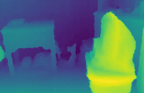
To accomplish this, we study the imaging process of a DP pair and provide a mathematical model handling the intrinsic problem of depth from defocus blur for a DP pair. Our method can jointly recover an all-in-focus image and estimate the depth of a scene (see Fig. 1). Our contributions are summarised as follows:
-
1.
We propose a theoretical DP model to explicitly define the relationship between depth, defocus blur and all-in-focus image;
-
2.
We design an end-to-end DP-based Depth and Deblur Network (DDDNet) to jointly estimate the depth map and restore the sharp image;
-
3.
We formulate a reblur loss based on our DP model which is used to regularise depth estimate in training;
-
4.
We create a DP image simulator, which enables us to create DP datasets from any RGB-D dataset;
-
5.
We collect a real dataset to stimulate further research.
Extensive experimental evaluation on both synthetic and real data shows that our approach achieves competitive performance compared to state-of-the-art approaches.
2 Related Work
For space reasons, we briefly review depth estimation from monocular, stereo, DP, and defocus.
Monocular. Supervised monocular depth estimation methods typically rely on large training datasets [20, 8]. Self-supervised methods [26, 29, 18, 11] often use estimated depths and camera poses to generate synthesized images, serving as supervision signals.
Stereo. To summarize, a stereo depth estimation network [12, 36, 23, 6, 35, 2, 34] often contains: matching cost computation, cost aggregation, and disparity optimization. Recently, several speed-up methods [32, 34] are available.
Dual-pixel. A DP pair has defocus blur and tiny baseline. To tackle the tiny baseline, Wadhwa et al. [31] utilize a small search size in block matching. Garg et al. [9] present the first learning models for affine invariant depth estimation to tackle affine ambiguity. Zhang et al. [38] present a Du2Net that uses a wide baseline stereo camera to compensate for the DP camera. However, it is specifically tailored for the ‘Google Pixel’ (narrow aperture, small DoF). The above three methods ignored the blur cue that could in principle fill in the parts where the disparity is imprecise (due to the tiny baseline). To tackle the defocus blur in a DP pair, Abuolaim et al. [1] first propose a DPDNet that remove the blur effect blindly. Recently, Punnappurath et al. [24] use a point spread function (PSF) to model the defocus blur and formulate the DP disparity by the PSF. However, the symmetry assumption of the PSF (only holds for constant depth region) limits its application for real-world scenario. Moreover, the method is time-consuming and has three steps (not end-to-end). In contrast, we study the imaging process of a DP pair and give a mathematical model jointly handling the intrinsic problem of depth from defocus blur for a DP pair.
Depth from defocus and deblurring. Depth from defocus has the same geometric constraints as disparity but different physiological constraints [7]. The estimated depth, also dubbed as defocus map, is commonly used to guide the deblurring [3, 28, 33, 21, 39, 19, 15]. DMENet [17] proposes the first end-to-end CNN architecture to estimate a spatially varying defocus map and use it for deblurring.
DP data. Only Canon and Google provide DP data to customers though most DSLR and smartphone cameras have the DP sensor. Several researchers [31, 9, 38] use ‘Google Pixel’ to collect data. However, smartphone cameras use a fixed and narrow aperture that cannot be adjusted. Canon is used in [1, 25, 24] with different aperture sizes, but it is expensive. Both of the two sensors are hard to get the associated GT information, such as depth. In parallel, the rise of deep learning has led to an explosion of demands for data. In this paper, we present the first DP simulator that synthesizes DP images with GT, from any RGB-D data.
3 Dual-Pixel Image Formation
In this section, we first discuss the formation of the two DP images and the defocus blur in Section 3.1. Then, in Section 3.2, we present our DP model and explore how to synthesize DP images from the RGB-D image. Based on the DP model, we build a DP simulator in Section 3.3.
3.1 Model of a dual-pixel camera
A DP camera can be modelled as an ordinary camera with a lens satisfying the thin-lens model, in which two (or more) images and are simultaneously captured. Here, the subscripts L and R denote the left and right view separately. In the model, the focal plane of the camera can be considered as consisting of two identically placed focal planes, one of which captures light rays coming from the left side of the lens, and the other captures light from the right side of the lens. The two images, and , can be considered as images taken by two different (but coplanar) lens, corresponding to regions in the aperture of a thin-lens.
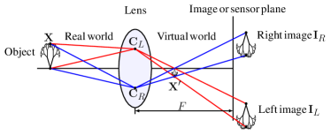
To be general, let it be assumed that the light for image passes through a region of the lens, and that for image comes from a region . Let us consider the case where and are infinitesimally small, consisting of just two points and (see Fig. 2). Choose a coordinate frame such that the lens lies on the plane , and the centre of the lens is at the origin. In addition, let the “world” lie to the left of the lens (that is with points ), and the camera lie to the right of the lens. Let consisting of points 111All vectors will be column vectors. with , and let be the 3D image of the virtual world, created by the lens, lying to the right of the lens. In particular, if , then . Here, is the focal length of the lens. Consider a plane of sensors (called a focal plane) lying inside the camera. Assume that this is parallel to the lens, so it is a plane defined by the equation , with . The symbol of is chosen to imply that this is the distance of the focal plane from the lens, but it is not the same as the focal length of the lens, which is .
Observation. An image of the world formed from rays passing through a point in the focal plane is the same as a pin-hole camera image of the virtual world with projection centre and the same focal plane. The same statement is true for the image formed from rays passing through .
Proof.
Refer to Fig. 2. Consider a world point , mapped by the lens to a virtual world point . This means that if is any point on the lens, then the ray is refracted by the lens to the ray . In particular, this is true for the point lying on the lens. Let the point be the point where the ray (extended if necessary) meets the focal plane. Then is the point where is imaged in . This is because a ray traverses the path , passing through on the way. On the other hand, looked at in terms of the pinhole camera with centre , the ray from to meets the focal plane at . This means that is the image of the point in the pinhole image taken from . ∎
Therefore, if the two regions were single points and , then the two images and are exactly a stereo pair of images of the virtual world . Although the two points and are necessarily very close together, the virtual world is also very small and very close to the camera lens, so there will be appreciable disparity.
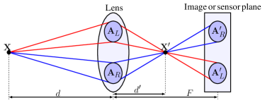
Non-pinhole model. In the case where the two regions and are bigger than a pinhole, and in fact constitute half the lens itself, the images and formed will be made up as the superposition of images of the virtual world taken at all points in region and in region . They will consequently be blurred. This is shown in Fig. 3.
Therefore, the problem of finding depth in the scene from images and is equivalent to doing stereo from blurred images. This will have its problems. The blur will be depth dependent. Points in the virtual world that lie on the focal plane will be in focus at independent of the position of the point and . Thus, points in the world corresponding to this placement of the focal plane will be both in focus and identically positioned in the two images and . Points that lie off the focal plane will be blurred and at the same time displaced by a disparity.
3.2 Image synthesis from RGB-D image
Given an image with an associated depth map, it is possible to synthesize either of the pair of dual-pixel images. Consider the image , formed from all rays passing through a region in the plane of the lens. (Note, is either or , and the corresponding image is either or .)
Let be an RGB-D image of the world, taken nominally from the viewpoint of the lens centre. Since the lens is normally very small with respect to the world, it will be assumed that any world point visible from the lens centre will be visible from any other point on the lens.
The RGB-D image gives us 3D coordinates of any point visible in the image. Let be such a point. The image of this point in the virtual world is given by
| (1) |
This point is then projected from each point onto the focal plane . The projection rays, through from points in form a cone with cross-section and vertex . This cone meets the focal plane in a further cross-section , Since the lens and focal plane are parallel, and will be similar regions, in the sense that there is a similarity transform relating and . Even more, this is simply a scaling and translation (where the scale may be positive or negative). In particular, a point maps to a point . Here, is a 2-dimensional offset and is a scale. For a given point , the values of and are constant, not dependent on the particular point chosen, but they vary according to the point chosen.
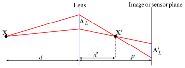
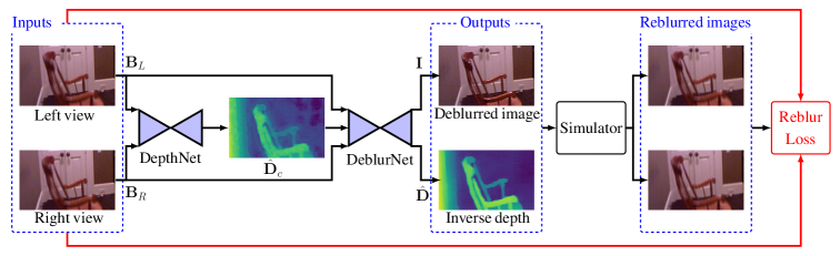
Image coordinates. We start with an RGB-D image, so each pixel in an image comes with an associated depth. For simplicity, we assume that all distances (including depth) are measured in pixel coordinates.
We make the following assumptions. A pixel with coordinates 222It is convenient to use for image coordinates, instead of the usual . corresponds with a ray in space defined by for varying . In particular, since each point in the image comes with a depth, we are assuming that the point imaged at point has 3D coordinates . This corresponds to a pinhole camera with focal plane given by and camera centre (pinhole) at the origin.
A point at depth will be mapped to a point , where , or
| (3) |
Let be a point in (lying on the lens plane ). The line from through is expressed as for varying values of . This line meets the plane when . The coordinates of this point are therefore
| (4) |
We are only interested in the -coordinates, in which case we have
| (5) |
Here, the transformation function for the left and right image has been defined with points and in and respectively.
3.3 DP simulator
Given a sharp image and its associated depth map , we can simulate a DP image pair as follows. Here, and are the image height and width, and it is also assumed that focal length and focal-plane-sensor distance are known (measured in units of pixel-size).
For each pixel in , as shown in Fig. 4 the intensity of a pixel is spread over regions and , in the left and right view of the DP pair. Each region contains a set of points , containing pixels, and the intensity of the pixel is spread out evenly over this set of pixels. Now running over all pixels , and summing, a pair of dual-pixel images are created. This is essentially blurring with depth-dependent blur kernel.
This operation is expensive computationally, since it requires looping over each pixel in the image, as well as each pixel in the region , thus levels of looping.
We utilize the concept of ‘integral image’ to speed up the computation, so that it has complexity independent of the size of the region , thus of order where is the number of pixels. In this description, we assume that the left and right halves of the aperture are approximated by rectangles, though with some amount of extra computation, more general shapes may be accommodated.
Given a pixel of the RGB-D image at a given depth, its corresponding light rays will pass through every point of . To compute the blur-region , one needs only to compute the destinations of the rays passing through the four corners of , which will be denoted by , , and in the left image . The positions of these four points are given by Eq. (5). Here, the subscript tl, tr, bl and br denotes top-left, top-right, bottom-left and bottom-right, respectively.
We create a differential mask for the region defined by
| (6) | ||||||
These values are summed for the regions corresponding to all points in the image, to create the differential image. Finally, we integrate the differential image, and the left/right view of the DP image pair is given by
| (7) |
where denotes the integral process. The integration process [30] is also closely related to ‘summed area tables’ in graphics [5].
Our simulator allows the vision community to collect large amounts of DP data with ground truth, opening the door to accurately benchmark DP-based methods. Our simulator can also be used to supervise the learning process.
With the DP model and the simulator, we build our DDDNet considering both stereo and defocus cues.
4 DP-based Depth and Deblur Network
4.1 Network architecture.
The input of our DDDNet is the left and right view of a DP image pair . The output of our DDDNet is the estimated inverse depth map and the deblurred image . We use ground-truth latent sharp image and inverse depth map for training.
The pipeline of DDDNet is shown in Fig. 5. It consists of two components: DepthNet with parameters and DeblurNet with parameters . The DepthNet is based on [4] and the DeblurNet is based on the multi-patch network [37]. Note that our approach is independent to the choices of and (\eg, multi-scale and multi-patch architectures). We start with a coarse inverse depth map estimation by the DepthNet, where . Then, we combine the coarse and blurred inverse depth map with , and feed it to the DeblurNet. The DeblurNet is an encoder-decoder network, and .
4.2 Loss functions.
We use a combination of an image restoration loss, depth loss, and an image reblur loss. The final loss is a sum of the three losses.
| (8) |
Image restoration loss . This loss ensures the deblurred image is similar to the target image, and is given by
| (9) |
where is the number of pixels and is the norm.
Depth loss . We adopt the smooth loss. Smooth loss is widely used in a regression task, for its robustness and low sensitivity to outliers [10]. The is defined as
| (10) |
Image reblur loss . The reblur loss penalizes the differences between the input blurred images and the reblurred images (from the DP simulator). The reblur loss explicitly enforces the restored image and inverse depth map to lie on the manifold of the ground-truth image and inverse depth map, subject to our DP model. The is given by
| (11) |
|
 |
 |
|---|---|---|
| (a) Input image | (b) GT: Depth | (c) BTS [18] |
|
 |
 |
| (d) SDoF [31] | (e) DPdisp [24] | (f) Ours |
DPD-blur EBDB [15] DMENet [17] DPDNet [1] Ourswb/Oursreb PSNR 24.82 23.93 25.53 26.15/26.76 SSIM 0.801 0.812 0.826 0.827/0.842 MSE_rel 5.74 6.36 5.29 4.93/4.59 Our-syn PSNR 26.48 30.14 31.45 32.17/33.21 SSIM 0.891 0.939 0.926 0.948/0.956 MSE_rel 4.74 3.11 2.68 2.46/2.17 Our-real PSNR 21.67 23.18 22.65 23.99/24.03 SSIM 0.763 0.809 0.808 0.826/ 0.850 MSE_rel 8.25 6.39 7.09 6.24/ 6.13
Sensor Method abs_rel sq_rel rmse rmse_log PSNR Monocular BTS [18] 0.377 0.195 0.255 0.484 0.554 0.741 0.994 - Stereo AnyNet [32] 0.128 0.117 0.731 0.168 0.828 0.923 0.998 - Dual-pixel DPdisp [24] 0.328 0.479 1.252 0.332 0.438 0.804 0.965 - Oursb 0.149 0.364 1.222 0.224 0.743 0.930 0.978 - Ourswb 0.091 0.082 0.599 0.123 0.918 0.993 0.998 32.171 Oursreb 0.083 0.052 0.461 0.111 0.936 0.998 1.000 33.218
5 Experiment
5.1 Experimental setup
Real dataset. We evaluate our method on three real DP datasets, namely, the Defocus Depth estimation dataset (DPD-disp) [24], Defocus Deblur Dual-Pixel dataset (DPD-blur) [1], and our new-collected dataset (Our-real) . DPD-disp dataset provides DP images with depth maps. The ground-truth (GT) depth map is computed by applying the well-established depth-from-defocus technique. DPD-blur provides a collection of image pairs captured by Canon 5D IV with all-in-focus and out-of-focus. Compared with the DPD-blur dataset, Our-real is collected by Canon with a variety of aperture sizes, varying from to . Each all-in-focus image is associated with several out-of-focus blurred images, yielding a diversity dataset. Our-real contains 150 scenes, including both indoor and outdoor scenes, captured under a variety of lighting conditions.
Synthetic dataset. Our synthetic dataset is generated using the proposed DP simulator. We use the NYU depth dataset [22] as the input to our simulator, as it provides RGB images with depths. Giving different camera parameters, we simulate 5000 image pairs for training and 500 image pairs for testing.
Evaluation metrics. Given a DP-pair, our method jointly estimates a depth map and a deblurred image. We use standard metrics to evaluate the quality of estimated depth map and restored image separately. For depth map, we use absolute relative error ‘Abs_Rel’, square relative error ‘Sq_Rel’, root mean square error ‘RMSE’ and its log scale ‘RMSE_log’, and the inlier ratios (maximal mean relative error of for ). For restored image, we adopt the peak signal-to-noise ratio ‘PSNR’, structural similarity ‘SSIM’, and RMSE relative error ‘RMSE_rel’. For the DPD-disp dataset, we follow DPdisp [24] to use the affine invariant version of MAE ( ‘AI(1)’), RMSE (‘AI(w)’), and Spearman’s rank correlation (‘’) for evaluation.
Baseline methods. For depth map, we compare with state-of-the-art monocular (BTS [18], Monodepth2 [11]), stereo (AnyNet [32]), and DP (SDoF [31], DPdisp [24]) based depth estimation methods. For defocus deblurring, we compared with EBDB [15], DMENet [17], and DPDNet [1]. All methods are evaluated on each dataset independently. All learning methods are fine-tuned for each dataset (except DPD-disp, as no training data is provided). To fine-tune DMENet [17] on the DPD-blur and Our-real dataset, we use BTS [18] to estimate a coarse depth map to train, as the two datasets do not provide ground-truth depth maps. The same coarse depth maps are also used to train our network.
Implementation details. Our network is implemented in Pytorch and is trained from scratch using the Adam optimizer [16] with a learning rate of and a batch size of . Our model is trained on a single NVIDIA Titan XP GPU. The code and data will be released.
|
 |
 |
 |
 |
|---|---|---|---|---|
|
 |
 |
 |
 |
|
 |
 |
 |
 |
|
 |
 |
 |
 |

|
 |
 |
 |
 |
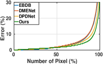
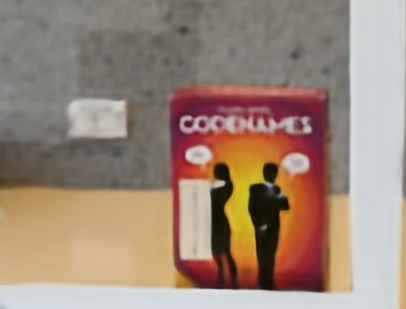
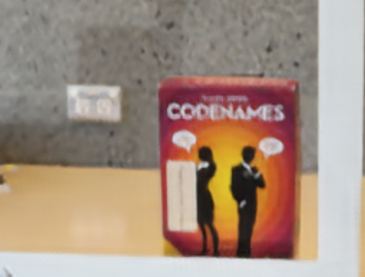
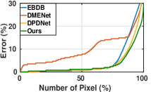
| (a) Input image | (b) GT image | (c) Intensity error | (d) DPDNet [1] | (e) Ours: |
|
 |
 |
 |
 |
 |
|---|---|---|---|---|---|
| (a) GT: Image | (b) Input image | (c) EBDB [15] | (d) DMENet [17] | (e) DPDNet [1] | (f) Ourswb: |
|
 |
 |
 |
 |
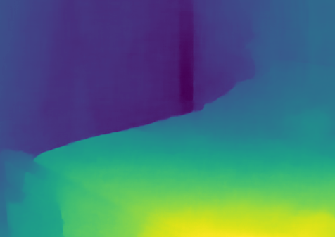 |
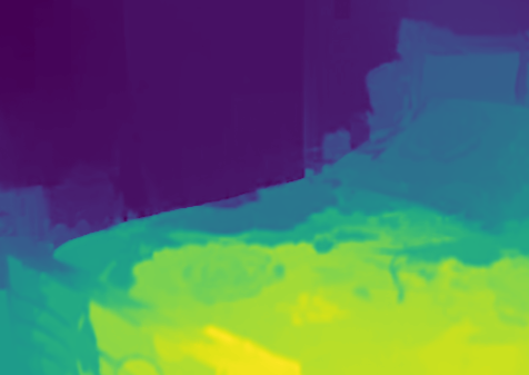
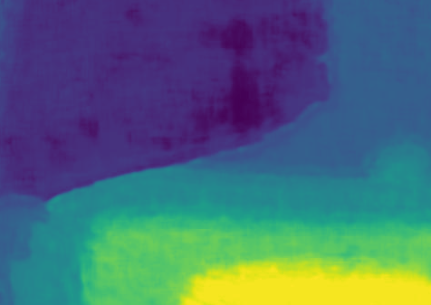
| (g) GT: inverse depth | (h) BTS [18] | (i) AnyNet [32] | (j) DPdisp [24] | (k) Oursb: | (l) Oursreb: |
|
 |
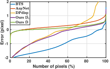
|---|---|
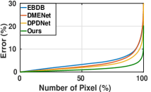
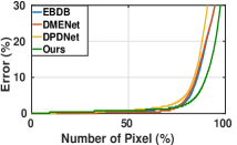
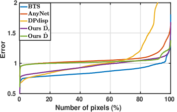
| (m) Inverse depth error, | (n) Inverse depth error, |
5.2 Results and discussions
We compare our results with baselines on depth estimation and image deblurring on 4 (including real and synthetic) datasets.
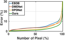
Deblurring results. We show the quantitative and qualitative comparisons for deblurring in Table 1, Fig. 7 and Fig. 8, respectively. In Table 1, we achieve competitive results compared with the state-of-the-art methods [15, 17, 1] on both DPD-blur, Our-syn, and Our-real dataset. Here, ‘Ourswb’ and ‘Oursreb’ denote results without and with the reblur loss, respectively. The relative improvement is around , demonstrating that using our DP-model based reblur loss can significantly improve the deblurring performance of our DDDNet. Fig. 7 and Fig. 8 show the qualitative and quantitative comparisons on the three datasets.
Depth results. We first provide depth estimation results on the DPD-disp dataset. The comparisons are shown in Table 2 and Fig. 6. As no training data is available, we directly test our model (trained on Our-syn dataset) on their testing set without fine-tuning and achieve the second best performance. Furthermore, note that our DP-model based reblur loss can be used as a ‘self-supervision’ signal to adapt our DDDNet to this test dataset, we can further fine-tune our model trained on Our-syn dataset using our reblur loss, without using GT depth map. Our model with reblur loss ‘Ours (fine-tune)’ achieves competitive results compared with the state-of-the-art methods [18, 11, 31, 24].
We then provide depth comparisons on Our-syn dataset. The results are shown in Table 3 and Fig. 8. In Table 3, we evaluate the outputs of our DDDNet step by step, it shows that, with our joint optimization of depth estimation and deblurring, we improve the quality of both the depth map and the deblurred image. Also, with our DP-model based reblur loss, we further improve our performance. For example, for the ‘abs_rel’ metric, the relative error for the coarse depth map as the output of the DepthNet (see Fig. 5), the DeblurNet without reblur loss and the DeblurNet with reblur loss is , and , respectively.
Effectiveness of our simulated DP images. To further show the usefulness of our simulated DP images, our model trained on Our-syn dataset is directly used to test on the DPD-blur dataset. The result is dB// in PSNR/SSIM/RMSE_rel without any fine-tuning. After fine-tuning, our model trained on Our-syn get remarkable performance, with PSNR/SSIM/RMSE_rel at dB//, outperforming the performance of our model (dB//) directly trained on the DPD-blur dataset. To further show the transfer ability of our model trained using simulated DP images, we only use a half amount of images from the DPD-blur dataset to finetune our model trained on Our-syn dataset, obtaining a good performance, with PSNR/SSIM/RMSE_rel at dB// in epoches.
6 Conclusions
In this paper, we derive a mathematical DP model formulating the imaging process of the DP camera. We propose an end-to-end DDDNet (DP-based Depth and Deblur Network), to jointly estimate a inverse depth map and restore a sharp image from a blurred DP image pair. Also, we present a reblur loss building upon our DP model and integrate it into our DDDNet. For future work, we plan to extend our DDDNet to a self-supervised depth and sharp image estimation network.
References
- [1] Abdullah Abuolaim and Michael S Brown. Defocus deblurring using dual-pixel data. arXiv preprint arXiv:2005.00305, 2020.
- [2] Filippo Aleotti, Fabio Tosi, Li Zhang, Matteo Poggi, and Stefano Mattoccia. Reversing the cycle: self-supervised deep stereo through enhanced monocular distillation. arXiv preprint arXiv:2008.07130, 2020.
- [3] Ching-Hui Chen, Hui Zhou, and Timo Ahonen. Blur-aware disparity estimation from defocus stereo images. In Proceedings of the IEEE International Conference on Computer Vision, pages 855–863, 2015.
- [4] Xuelian Cheng, Yiran Zhong, Mehrtash Harandi, Yuchao Dai, Xiaojun Chang, Tom Drummond, Hongdong Li, and Zongyuan Ge. Hierarchical neural architecture search for deep stereo matching. arXiv preprint arXiv:2010.13501, 2020.
- [5] Franklin C Crow. Summed-area tables for texture mapping. In Proceedings of the 11th annual conference on Computer graphics and interactive techniques, pages 207–212, 1984.
- [6] Shivam Duggal, Shenlong Wang, Wei-Chiu Ma, Rui Hu, and Raquel Urtasun. Deeppruner: Learning efficient stereo matching via differentiable patchmatch. In Proceedings of the IEEE/CVF International Conference on Computer Vision (ICCV), October 2019.
- [7] John Ens and Peter Lawrence. An investigation of methods for determining depth from focus. IEEE Transactions on pattern analysis and machine intelligence, 15(2):97–108, 1993.
- [8] Huan Fu, Mingming Gong, Chaohui Wang, Kayhan Batmanghelich, and Dacheng Tao. Deep ordinal regression network for monocular depth estimation. In Proceedings of the IEEE Conference on Computer Vision and Pattern Recognition, pages 2002–2011, 2018.
- [9] Rahul Garg, Neal Wadhwa, Sameer Ansari, and Jonathan T Barron. Learning single camera depth estimation using dual-pixels. In Proceedings of the IEEE International Conference on Computer Vision, pages 7628–7637, 2019.
- [10] Ross Girshick. Fast r-cnn. In Proceedings of the IEEE international conference on computer vision, pages 1440–1448, 2015.
- [11] Clément Godard, Oisin Mac Aodha, Michael Firman, and Gabriel J Brostow. Digging into self-supervised monocular depth estimation. In Proceedings of the IEEE international conference on computer vision, pages 3828–3838, 2019.
- [12] Rostam Affendi Hamzah and Haidi Ibrahim. Literature survey on stereo vision disparity map algorithms. Journal of Sensors, 2016, 2016.
- [13] Charles Herrmann, Richard Strong Bowen, Neal Wadhwa, Rahul Garg, Qiurui He, Jonathan T Barron, and Ramin Zabih. Learning to autofocus. In Proceedings of the IEEE/CVF Conference on Computer Vision and Pattern Recognition, pages 2230–2239, 2020.
- [14] Jinbeum Jang, Yoonjong Yoo, Jongheon Kim, and Joonki Paik. Sensor-based auto-focusing system using multi-scale feature extraction and phase correlation matching. Sensors, 15(3):5747–5762, 2015.
- [15] Ali Karaali and Claudio Rosito Jung. Edge-based defocus blur estimation with adaptive scale selection. IEEE Transactions on Image Processing, 27(3):1126–1137, 2017.
- [16] Diederick P Kingma and Jimmy Ba. Adam: A method for stochastic optimization. In International Conference on Learning Representations (ICLR), 2015.
- [17] Junyong Lee, Sungkil Lee, Sunghyun Cho, and Seungyong Lee. Deep defocus map estimation using domain adaptation. In Proceedings of the IEEE Conference on Computer Vision and Pattern Recognition, pages 12222–12230, 2019.
- [18] Jin Han Lee, Myung-Kyu Han, Dong Wook Ko, and Il Hong Suh. From big to small: Multi-scale local planar guidance for monocular depth estimation. arXiv preprint arXiv:1907.10326, 2019.
- [19] Anat Levin, Rob Fergus, Frédo Durand, and William T Freeman. Image and depth from a conventional camera with a coded aperture. ACM transactions on graphics (TOG), 26(3):70–es, 2007.
- [20] Fayao Liu, Chunhua Shen, Guosheng Lin, and Ian Reid. Learning depth from single monocular images using deep convolutional neural fields. IEEE transactions on pattern analysis and machine intelligence, 38(10):2024–2039, 2015.
- [21] Maxim Maximov, Kevin Galim, and Laura Leal-Taixé. Focus on defocus: bridging the synthetic to real domain gap for depth estimation. In Proceedings of the IEEE/CVF Conference on Computer Vision and Pattern Recognition, pages 1071–1080, 2020.
- [22] Pushmeet Kohli Nathan Silberman, Derek Hoiem and Rob Fergus. Indoor segmentation and support inference from rgbd images. In Proceedings of the European Conference on Computer Vision (ECCV), 2012.
- [23] Guang-Yu Nie, Ming-Ming Cheng, Yun Liu, Zhengfa Liang, Deng-Ping Fan, Yue Liu, and Yongtian Wang. Multi-level context ultra-aggregation for stereo matching. In Proceedings of the IEEE/CVF Conference on Computer Vision and Pattern Recognition (CVPR), June 2019.
- [24] Abhijith Punnappurath, Abdullah Abuolaim, Mahmoud Afifi, and Michael S. Brown. Modeling defocus-disparity in dual-pixel sensors. In IEEE International Conference on Computational Photography (ICCP), 2020.
- [25] Abhijith Punnappurath and Michael S Brown. Reflection removal using a dual-pixel sensor. In Proceedings of the IEEE Conference on Computer Vision and Pattern Recognition, pages 1556–1565, 2019.
- [26] Ashutosh Saxena, Min Sun, and Andrew Y Ng. Learning 3-d scene structure from a single still image. In 2007 IEEE 11th International Conference on Computer Vision, pages 1–8. IEEE, 2007.
- [27] Przemysław Śliwiński and Paweł Wachel. A simple model for on-sensor phase-detection autofocusing algorithm. Journal of Computer and Communications, 1(06):11, 2013.
- [28] Supasorn Suwajanakorn, Carlos Hernandez, and Steven M Seitz. Depth from focus with your mobile phone. In Proceedings of the IEEE Conference on Computer Vision and Pattern Recognition, pages 3497–3506, 2015.
- [29] Fabio Tosi, Filippo Aleotti, Matteo Poggi, and Stefano Mattoccia. Learning monocular depth estimation infusing traditional stereo knowledge. In Proceedings of the IEEE/CVF Conference on Computer Vision and Pattern Recognition (CVPR), June 2019.
- [30] Paul Viola, Michael Jones, et al. Robust real-time object detection. International journal of computer vision, 4(34-47):4, 2001.
- [31] Neal Wadhwa, Rahul Garg, David E Jacobs, Bryan E Feldman, Nori Kanazawa, Robert Carroll, Yair Movshovitz-Attias, Jonathan T Barron, Yael Pritch, and Marc Levoy. Synthetic depth-of-field with a single-camera mobile phone. ACM Transactions on Graphics (TOG), 37(4):1–13, 2018.
- [32] Yan Wang, Zihang Lai, Gao Huang, Brian H Wang, Laurens Van Der Maaten, Mark Campbell, and Kilian Q Weinberger. Anytime stereo image depth estimation on mobile devices. In 2019 International Conference on Robotics and Automation (ICRA), pages 5893–5900. IEEE, 2019.
- [33] Guodong Xu, Yuhui Quan, and Hui Ji. Estimating defocus blur via rank of local patches. In Proceedings of the IEEE International Conference on Computer Vision, pages 5371–5379, 2017.
- [34] Haofei Xu and Juyong Zhang. Aanet: Adaptive aggregation network for efficient stereo matching. In Proceedings of the IEEE/CVF Conference on Computer Vision and Pattern Recognition, pages 1959–1968, 2020.
- [35] Zhichao Yin, Trevor Darrell, and Fisher Yu. Hierarchical discrete distribution decomposition for match density estimation. In Proceedings of the IEEE/CVF Conference on Computer Vision and Pattern Recognition (CVPR), June 2019.
- [36] Jure Žbontar and Yann LeCun. Stereo matching by training a convolutional neural network to compare image patches. The journal of machine learning research, 17(1):2287–2318, 2016.
- [37] Hongguang Zhang, Yuchao Dai, Hongdong Li, and Piotr Koniusz. Deep stacked hierarchical multi-patch network for image deblurring. In Proceedings of the IEEE Conference on Computer Vision and Pattern Recognition (CVPR), June 2019.
- [38] Yinda Zhang, Neal Wadhwa, Sergio Orts-Escolano, Christian Häne, Sean Fanello, and Rahul Garg. Du2net: Learning depth estimation from dual-cameras and dual-pixels. arXiv preprint arXiv:2003.14299, 2020.
- [39] Shaojie Zhuo and Terence Sim. Defocus map estimation from a single image. Pattern Recognition, 44(9):1852–1858, 2011.