Near-Optimal Control Strategy in Leader-Follower Networks: A Case Study for Linear Quadratic Mean-Field Teams

Abstract

In this paper, a decentralized stochastic control system consisting of one leader and many homogeneous followers is studied. The leader and followers are coupled in both dynamics and cost, where the dynamics are linear and the cost function is quadratic in the states and actions of the leader and followers. The objective of the leader and followers is to reach consensus while minimizing their communication and energy costs. The leader knows its local state and each follower knows its local state and the state of the leader. The number of required links to implement this decentralized information structure is equal to the number of followers, which is the minimum number of links for a communication graph to be connected. In the special case of leaderless, no link is required among followers, i.e., the communication graph is not even connected. We propose a near-optimal control strategy that converges to the optimal solution as the number of followers increases. One of the salient features of the proposed solution is that it provides a design scheme, where the convergence rate as well as the collective behavior of the followers can be designed by choosing appropriate cost functions. In addition, the computational complexity of the proposed solution does not depend on the number of followers. Furthermore, the proposed strategy can be computed in a distributed manner, where the leader solves one Riccati equation and each follower solves two Riccati equations to calculate their strategies. Two numerical examples are provided to demonstrate the effectiveness of the results in the control of multi-agent systems.

Proceedings of IEEE Conference on Decision and Control, 2018.

I Introduction

The control of multi-agent systems with leader-follower structure has attracted much interest in the past two decades due to its wide range of applications in various fields of science and engineering. Such applications include vehicle formation [1], sensor networks [2], surveillance using a team of unmanned aerial vehicles (UAVs) [3] and flocking [4, 5], to name only a few. In this type of problem, a group of agents (called followers) are to track an agent (called leader) while certain performance objectives are achieved. Different performance measures such as minimum energy, fuel or time are considered in the literature. For this purpose, limited communication and computation resources are two main challenges that need to be overcome.

To address the challenges outlined in the previous paragraph, the following two problems have been investigated in the context of consensus control protocols in the literature recently: (i) how the states of the followers can reach the state of the leader under communication constraints (distributed control problem), where consensus is reached under appropriate linear strategies for properly connected communication graphs [6, 7, 8], and (ii) how the state of the followers can reach the state of the leader with minimum energy consumption (optimal control problem), where the optimal control strategy for a quadratic performance index with linear dynamics under centralized information structure is a linear feedback rule obtained by the solution of the celebrated Riccati equation [9]. Combining the above two objectives, however, is quite challenging as it leads to a decentralized optimal control problem wherein the optimal control law is not necessarily linear [10]. Furthermore, since the dimension of the matrices in the network model increases with the number of followers, the optimal control law may be intractable for a network of large size. In this paper, we consider a decentralized optimal control problem with a large number of followers.

For dynamically decoupled followers and also the case of a leaderless multi-agent system, [11, 12] use the control inverse optimality approach to compute the optimal distributed control strategies for special classes of communication graphs. The authors in [13] consider a large number of homogeneous followers and determine the optimal strategy by solving two coupled Riccati equations. In contrast, this paper studies a leader-follower multi-agent network with coupled dynamics under a directed communication graph in which there is a direct link from the leader to each follower. In the special case of leaderless, the communication graph is not required to be connected. When the initial states of followers are identically and independently distributed, a near-optimal strategy is proposed for a large number of homogeneous followers by solving two decoupled Riccati equations using mean-field team approach introduced by [14] and showcased in [15, 16, 17, 18].

The remainder of this paper is organized as follows. The problem is formulated in the next section, where the main contributions of the work are also outlined. Then in Section III, some important assumptions are presented and the control strategy is derived. Two numerical examples are provided in Section IV and finally the paper is concluded in Section V.

II Problem Formulation

II-A Notation

In this paper, $\mathbb{N}$ and $\mathbb{R}$ denote natural and real numbers, respectively. The short-hand notation $x_{a:b}$ is used to denote vector $(x_{a},\ldots,x_{b})$, $a\leq b\in\mathbb{N}$. For any $k\in\mathbb{N}$, $\mathbb{N}_{k}$ is the finite set of integers $\{1,2,\ldots,k\}$. $\operatorname{Tr}(\bm{\cdot})$ is the trace of a matrix and $\operatorname{var}(\bm{\cdot})$ is the covariance of a random vector.

II-B Dynamics

Consider a multi-agent system consisting of one leader and $n\in\mathbb{N}$ followers. Denote by $x^{0}_{t}\in\mathbb{R}^{d_{x}},$ $u^{0}_{t}\in\mathbb{R}^{d_{u}}$, and $w^{0}_{t}\in\mathbb{R}^{d_{x}}$, $d_{x},d_{u}\in\mathbb{N}$, the state, action, and noise of the leader at time $t\in\mathbb{N}$, respectively. In addition, let $x^{i}_{t}\in\mathbb{R}^{d_{x}}$, $u^{i}_{t}\in\mathbb{R}^{d_{u}}$, and $w^{i}_{t}\in\mathbb{R}^{d_{x}}$ denote the state, action, and noise of follower $i\in\mathbb{N}_{n}$ at time $t\in\mathbb{N}$, analogously. The state of the leader evolves as follows:

$$x^{0}_{t+1}=A_{t}^{0}x^{0}_{t}+B_{t}^{0}u^{0}_{t}+D^{0}_{t}\bar{x}_{t}+w^{0}_{t},$$ (1)

where $\bar{x}_{t}:=\frac{1}{n}\sum_{i=1}^{n}x^{i}_{t}$ is the average of the states of the followers at time $t$, and will hereafter be called mean-field [14]. Similarly, the state of each follower $i\in\mathbb{N}_{n}$ evolves as follows:

$$x^{i}_{t+1}=A_{t}x^{i}_{t}+B_{t}u^{i}_{t}+D_{t}\bar{x}_{t}+E_{t}x_{t}^{0}+w^{i}_{t}.$$ (2)

Let $\mathbb{N}_{T}$, $T\in\mathbb{N},$ be the control horizon. It is assumed that the primitive random variables $\{x^{0}_{1},x^{1}_{1},\ldots,x^{n}_{1},w^{0}_{1},w^{1}_{1},\ldots,w^{n}_{1},\ldots,w^{0}_{T},w^{1}_{T},\ldots,w^{n}_{T}\}$ are defined on a common probability space, and are mutually independent.

II-C Information structure

At time $t\in\mathbb{N}$, the leader observes its state $x^{0}_{t}$ and chooses its action $u^{0}_{t}$ according to a control law $g^{0}_{t}:\mathbb{R}^{d_{x}}\rightarrow\mathbb{R}^{d_{u}}$, i.e.,

$$u^{0}_{t}=g^{0}_{t}(x^{0}_{t}).$$ (3)

In addition, for any $i\in\mathbb{N}_{n}$, follower $i$ observes its state $x^{i}_{t}$ as well as the state of the leader $x^{0}_{t}$ at time $t$, and decides its action $u^{i}_{t}$ as follows:

$$u^{i}_{t}=g^{i}_{t}(x^{i}_{t},x^{0}_{t}),$$ (4)

where $g^{i}_{t}:\mathbb{R}^{d_{x}}\times\mathbb{R}^{d_{x}}\rightarrow\mathbb{R}^{d_{u}}$ is the control law. Note that the control actions (3) and (4) have a non-classical decentralized information structure.

Remark 1

The number of links required to implement the above information structure is $n$, which is the minimum possible number of links for leader-follower networks to be connected. In addition, no information about the states of the followers is communicated; hence, the privacy of the followers is preserved. _□

Remark 2

It is worth highlighting the difference between the dynamics coupling (1) and (2), that refers to the physical interactions among agents, and information coupling (3) and (4), that attributes to the communication of data. _□

The set of all control laws $\mathbf{g}:=\{g^{0}_{1:T},g^{1}_{1:T},\ldots,g^{n}_{1:T}\}$ is called the strategy of the network. The objective of the followers is to track the leader in an energy-efficient manner. To this end, the following cost function is defined:

$$J_{T}(\mathbf{g})=\mathbb{E}\Big{[}\sum_{t=1}^{T}(x^{0}_{t})^{\intercal}Q^{0}_{t}x^{0}_{t}+(\bar{x}_{t}-x^{0}_{t})^{\intercal}F_{t}(\bar{x}_{t}-x^{0}_{t})+(u^{0}_{t})^{\intercal}R^{0}_{t}u^{0}_{t}$$

$$\quad+\frac{1}{n}\sum_{i=1}^{n}(x^{i}_{t})^{\intercal}Q_{t}x^{i}_{t}+(x^{i}_{t}-x^{0}_{t})^{\intercal}P_{t}(x^{i}_{t}-x^{0}_{t})+(u^{i}_{t})^{\intercal}R_{t}u^{i}_{t}$$

$$\quad+\frac{1}{2n^{2}}\sum_{i=1}^{n}\sum_{j=1}^{n}(x^{i}_{t}-x^{j}_{t})^{\intercal}H_{t}(x^{i}_{t}-x^{j}_{t})\Big{]},$$ (5)

where the expectation is taken with respect to the probability measures induced by the choice of strategy $\mathbf{g}$, and $\{Q^{0}_{t},F_{t},R^{0}_{t},Q_{t},P_{t},R_{t},H_{t}\}$ are symmetric matrices of appropriate dimensions. It is to be noted that the rate of convergence of the followers to the leader depends on the matrices $P_{t}$ and $F_{t}$. Moreover, the collective behavior of the followers changes by matrix $H_{t}$.

Problem 1

Consider the above leader-follower system with dynamics (1) and (2) and information structure (3) and (4). We are interested to find an $\varepsilon(n)$-optimal strategy $\mathbf{g}^{\ast}_{\varepsilon}$ such that for every strategy $\mathbf{g}$,

$$J_{T}(\mathbf{g}^{\ast}_{\varepsilon})\leq J_{T}(\mathbf{g})+\varepsilon(n),$$ (6)

where $\varepsilon(n)\in[0,\infty)$ and $\lim_{n\rightarrow\infty}\varepsilon(n)=0$.

Remark 3

Notice that if matrices $B^{0}_{t}$, $D^{0}_{t},Q^{0}_{t}$ and $R^{0}_{t}$ are zero, Problem 1 reduces to the optimal control of a leaderless multi-agent network. In that case, $x^{0}_{t}$ represents the desired reference trajectory, and as noted before, the followers do not share anything with each other once they receive the reference trajectory information $x^{0}_{t}$, according to (4). _□

II-D Main challenges and contributions

There are two main challenges in finding a solution to Problem 1. The first one is concerned with non-classical information structure, as the optimal strategy under this type of information structure is not necessarily linear [10]. The second challenge is the curse of dimensionality as the matrices in Problem 1 are fully dense, yet their dimension increases with the number of followers.

In their previous work [15], the authors show that if the mean-field $\bar{x}_{t}$ is available to the leader and followers, then the optimal solution is unique and linear. However, collecting and sharing the mean-field among all agents is not cost-efficient, in general, specially when the number of followers $n$ is large. It is shown in the next section that the effect of such information sharing on the performance of the network is negligible when the number of followers is large enough.

III Main Results

In this section, we propose a strategy and compute its performance with respect to the optimal performance, and show that the difference between them converges to zero at rate $\frac{1}{n}$. For the sake of clarity in the notation, we use letters $s$ and $v$ to denote the states and actions, respectively, under the optimal strategy. Therefore, from (1) and  (2), the dynamics of the leader and followers at time $t\in\mathbb{N}_{T}$ under the optimal strategy are given by

$$s^{0}_{t+1}=A_{t}^{0}s^{0}_{t}+B_{t}^{0}v^{0}_{t}+D^{0}_{t}\bar{s}_{t}+w^{0}_{t},$$ (7)

$$s^{i}_{t+1}=A_{t}s^{i}_{t}+B_{t}v^{i}_{t}+D_{t}\bar{s}_{t}+E_{t}s_{t}^{0}+w^{i}_{t},\quad i\in\mathbb{N}_{n},$$ (8)

where $\bar{s}_{t}:=\frac{1}{n}\sum_{i=1}^{n}s^{i}_{t}$. Similarly to [15], define the following matrices:

$$\bar{A}_{t}:=\left[\begin{array}[]{cc}A^{0}_{t}&D^{0}_{t}\\ E_{t}&A_{t}+D_{t}\end{array}\right],\quad\bar{B}_{t}:=\left[\begin{array}[]{cc}B^{0}_{t}&\mathbf{0}_{d_{x}\times d_{u}}\\ \mathbf{0}_{d_{x}\times d_{u}}&B_{t}\end{array}\right],$$ (9)

$$\bar{Q}_{t}:=\left[\begin{array}[]{cc}Q^{0}_{t}+P_{t}+F_{t}&-P_{t}-F_{t}\\ -P_{t}-F_{t}&Q_{t}+P_{t}+F_{t}\end{array}\right],\bar{R}_{t}:=\left[\begin{array}[]{cc}R^{0}_{t}&\mathbf{0}_{d_{u}\times d_{u}}\\ \mathbf{0}_{d_{u}\times d_{u}}&R_{t}\end{array}\right].$$ (10)

Assumption 1

Matrices $Q_{t}+P_{t}+H_{t}$ and $\bar{Q}_{t}$ are positive semi-definite and matrices $R_{t}$ and $R^{0}_{t}$ are positive definite.

Define two decoupled Riccati equations s.t. for any $t\in\mathbb{N}_{T}$,

$$\breve{M}_{t}=-A_{t}^{\intercal}\breve{M}_{t+1}B_{t}\left(B_{t}^{\intercal}\breve{M}_{t+1}B_{t}+R_{t}\right)^{-1}B_{t}^{\intercal}\breve{M}_{t+1}A_{t}\\ +A_{t}^{\intercal}\breve{M}_{t+1}A_{t}+Q_{t}+P_{t}+H_{t},$$ (11)

$$\bar{M}_{t}=-\bar{A}_{t}^{\intercal}\bar{M}_{t+1}\bar{B}_{t}\left(\bar{B}_{t}^{\intercal}\bar{M}_{t+1}\bar{B}_{t}+\bar{R}_{t}\right)^{-1}\bar{B}_{t}^{\intercal}\bar{M}_{t+1}\bar{A}_{t}\\ +\bar{A}_{t}^{\intercal}\bar{M}_{t+1}\bar{A}_{t}+\bar{Q}_{t},$$ (12)

where $\breve{M}_{T+1}=\mathbf{0}_{d_{x}\times d_{x}}$ and $\bar{M}_{T+1}=\mathbf{0}_{2d_{x}\times 2d_{x}}$. According to [14, 15], the optimal performance $J_{T}^{\ast}$ is obtained under the following linear strategies:

$${v^{0}_{t}} =\bar{L}^{1,1}_{t}s^{0}_{t}+\bar{L}^{1,2}_{t}\bar{s}_{t},$$ (13)

$${v^{i}_{t}} =\breve{L}_{t}s^{i}_{t}+\bar{L}_{t}^{2,1}s^{0}_{t}+(\bar{L}_{t}^{2,2}-\breve{L}_{t})\bar{s}_{t},$$ (14)

where $\breve{L}_{t}$ and $\bar{L}_{t}=:\left[\begin{array}[]{cc}\bar{L}^{1,1}_{t}&\bar{L}^{1,2}_{t}\\ \bar{L}^{2,1}_{t}&\bar{L}^{2,2}_{t}\end{array}\right]$ can be found by using these formulas:

$$\breve{L}_{t} =-\left(B_{t}^{\intercal}\breve{M}_{t+1}B_{t}+R_{t}\right)^{-1}B_{t}^{\intercal}\breve{M}_{t+1}A_{t},$$

$$\bar{L}_{t} =-\left(\bar{B}_{t}^{\intercal}\bar{M}_{t+1}\bar{B}_{t}+\bar{R}_{t}\right)^{-1}\bar{B}_{t}^{\intercal}\bar{M}_{t+1}\bar{A}_{t}.$$ (15)

III-A Solution of Problem 1

The following standard assumptions are imposed.

Assumption 2

The initial states of the followers are i.i.d. with mean $\mu_{x}\in\mathbb{R}^{d_{x}}$ and finite covariance matrix $\sum_{x}\in\mathbb{R}^{d_{x}}\times\mathbb{R}^{d_{x}}$. In addition, the local noises of the followers are i.i.d. with zero mean and finite covariance matrix $\sum_{w}\in\mathbb{R}^{d_{x}}\times\mathbb{R}^{d_{x}}$.

Assumption 3

Matrices $A_{t},A_{t}^{0},B_{t},B_{t}^{0},D_{t},D_{t}^{0},E_{t},F_{t},Q_{t}$, $Q_{t}^{0}$, $R_{t}$, $R_{t}^{0}$, $\sum_{x}$ and $\sum_{w}$ do not depend on the number of followers $n$.

Define a stochastic process $z_{1:T}$ such that $z_{1}:=\mu_{x}$ and for any $t\in\mathbb{N}_{T}$:

$$z_{t+1}=(A_{t}+B_{t}\bar{L}_{t}^{2,2}+D_{t})z_{t}+(B_{t}\bar{L}_{t}^{2,1}+E_{t})x_{t}^{0}.$$ (16)

Note that the leader and followers can compute $z_{t}$ under the information structures (3) and (4). Given the matrix gains defined in (III), the following strategies are proposed:

$$u_{t}^{0}=\bar{L}_{t}^{1,1}x_{t}^{0}+\bar{L}^{1,2}_{t}z_{t},$$ (17)

$$u_{t}^{i}=\breve{L}_{t}x_{t}^{i}+\bar{L}^{2,1}_{t}x_{t}^{0}+(\bar{L}^{2,2}_{t}-\breve{L}_{t})z_{t},\quad i\in\mathbb{N}_{n}.$$ (18)

At any time $t\in\mathbb{N}_{T}$, define the following relative errors $e_{t}^{0}$, $e_{t}$ and $\zeta_{t}$:

$$e_{t}^{0}:=s_{t}^{0}-x_{t}^{0},\quad e_{t}:=\bar{s}_{t}-z_{t},\quad\zeta_{t}:=\bar{x}_{t}-z_{t}.$$ (19)

Lemma 1

The relative errors defined in (19) evolve linearly in time as follows:

$$\left[\begin{array}[]{c}e_{t+1}^{0}\\ e_{t+1}\\ \zeta_{t+1}\end{array}\right]=\tilde{A}_{t}\left[\begin{array}[]{c}e_{t}^{0}\\ e_{t}\\ \zeta_{t}\end{array}\right]+\left[\begin{array}[]{c}\mathbf{0}_{d_{x}\times 1}\\ \bar{w}_{t}\\ \bar{w}_{t}\end{array}\right],$$ (20)

where $\bar{w}_{t}:=\frac{1}{n}\sum_{i=1}^{n}w^{i}_{t}$ and

$$\tilde{A}_{t}:=\left[\begin{array}[]{c c c}A_{t}^{0}+B_{t}^{0}\bar{L}_{t}^{1,1}&B_{t}^{0}\bar{L}_{t}^{1,2}+D_{t}^{0}&-D_{t}^{0}\\ B_{t}\bar{L}_{t}^{2,1}+E_{t}&A_{t}+B_{t}\bar{L}_{t}^{2,2}+D_{t}&\mathbf{0}_{d_{x}\times d_{x}}\\ \mathbf{0}_{d_{x}\times d_{x}}&\mathbf{0}_{d_{x}\times d_{x}}&A_{t}+B_{t}\breve{L}_{t}+D_{t}\end{array}\right].$$ (21)

_□

Proof

From (7) and (13):

$$s_{t+1}^{0}=(A_{t}^{0}+B_{t}^{0}\bar{L}^{1,1}_{t})s_{t}^{0}+(B_{t}^{0}\bar{L}_{t}^{1,2}+D_{t}^{0})\bar{s}_{t}+w_{t}^{0}.$$ (22)

Also, it results from (1) and (17) that

$$x_{t+1}^{0}=(A_{t}^{0}+B_{t}^{0}\bar{L}^{1,1}_{t})x_{t}^{0}+B_{t}^{0}\bar{L}_{t}^{1,2}z_{t}+D_{t}^{0}\bar{x}_{t}+w_{t}^{0}.$$ (23)

Similarly, from (8) and (14):

$$\bar{s}_{t+1}=A_{t}\bar{s}_{t}+B_{t}\bar{v}_{t}+D_{t}\bar{s}_{t}+E_{t}s_{t}^{0}+\bar{w}_{t},$$ (24)

where $\bar{v}_{t}:=\frac{1}{n}\sum_{i=1}^{n}v^{i}_{t}$ is given by:

$$\bar{v}_{t}=\breve{L}_{t}\bar{s}_{t}+\bar{L}_{t}^{2,1}s^{0}_{t}+(\bar{L}_{t}^{2,2}-\breve{L}_{t})\bar{s}_{t}=\bar{L}_{t}^{2,1}s^{0}_{t}+\bar{L}_{t}^{2,2}\bar{s}_{t}.$$ (25)

Substituting  (25) in  (24) yields:

$$\bar{s}_{t+1}=(A_{t}+B_{t}\bar{L}_{t}^{2,2}+D_{t})\bar{s}_{t}+(B_{t}\bar{L}_{t}^{2,1}+E_{t})s_{t}^{0}+\bar{w}_{t}.$$ (26)

In addition, from (2) and (18), one arrives at:

$$\bar{x}_{t+1}=A_{t}\bar{x}_{t}+B_{t}\bar{u}_{t}+D_{t}\bar{x}_{t}+E_{t}x_{t}^{0}+\bar{w}_{t},$$ (27)

where $\bar{u}_{t}:=\frac{1}{n}\sum_{i=1}^{n}u^{i}_{t}$ is as follows:

$$\bar{u}_{t+1}=\breve{L}_{t}\bar{x}_{t}+\bar{L}_{t}^{2,1}x_{t}^{0}+(\bar{L}_{t}^{2,2}-\breve{L}_{t})z_{t}.$$ (28)

From (27) and (28), it results that:

$$\bar{x}_{t+1}=A_{t}\bar{x}_{t}+B_{t}\breve{L}_{t}\bar{x}_{t}+B_{t}\bar{L}_{t}^{2,1}x_{t}^{0}+B_{t}(\bar{L}_{t}^{2,2}-\breve{L}_{t})z_{t}\\ +D_{t}\bar{x}_{t}+E_{t}x_{t}^{0}+\bar{w}_{t}.$$ (29)

Equations (19), (22) and (23) lead to:

$$e_{t+1}^{0} =(A_{t}^{0}+B_{t}^{0}\bar{L}_{t}^{1,1})s_{t}^{0}+B_{t}^{0}\bar{L}_{t}^{1,2}\bar{s}_{t}+D_{t}^{0}\bar{s}_{t}+w_{t}^{0}$$

$$\quad-(A_{t}^{0}x_{t}^{0}+B_{t}^{0}\bar{L}_{t}^{1,1}x_{t}^{0}+B_{t}^{0}\bar{L}_{t}^{1,2}z_{t}+D_{t}^{0}\bar{x}_{t}+w_{t}^{0})$$

$$=(A_{t}^{0}+B_{t}^{0}\bar{L}_{t}^{1,1})e_{t}^{0}+(B_{t}^{0}\bar{L}_{t}^{1,2}+D_{t}^{0})e_{t}-D_{t}^{0}\zeta_{t}.$$ (30)

Moreover, it results from  (16), (19) and (26) that:

$$e_{t+1} =A_{t}\bar{s}_{t}+B_{t}\bar{L}^{2,2}_{t}\bar{s}_{t}+D_{t}\bar{s}_{t}+B_{t}\bar{L}_{t}^{2,1}s_{t}^{0}+E_{t}s_{t}^{0}+\bar{w}_{t}$$

$$\quad-(A_{t}z_{t}+B_{t}\bar{L}_{t}^{2,2}z_{t}+D_{t}z_{t}+B_{t}\bar{L}_{t}^{2,1}x_{t}^{0}+E_{t}x_{t}^{0}),$$ (31)

$$=(A_{t}+B_{t}\bar{L}_{t}^{2,2}+D_{t})e_{t}+(B_{t}\bar{L}_{t}^{2,1}+E_{t})e_{t}^{0}+\bar{w}_{t}.$$ (32)

As a consequence of (16), (19) and (29), the following equation is obtained:

$$\zeta_{t+1}=(A_{t}+B_{t}\breve{L}_{t}+D_{t})\bar{x}_{t}+B_{t}(\bar{L}_{t}^{2,1}-\breve{L}_{t})x_{t}^{0}+B_{t}\bar{L}_{t}^{2,2}z_{t}$$

$$+E_{t}x_{t}^{0}+\bar{w}_{t}-(A_{t}+B_{t}\bar{L}_{t}^{2,2}+D_{t})z_{t}-(B_{t}\bar{L}_{t}^{2,1}+E_{t})x_{t}^{0}$$

$$\qquad=(A_{t}+B_{t}\breve{L}_{t}+D_{t})\zeta_{t}+\bar{w}_{t},$$ (33)

and this completes the proof. $\hfill\blacksquare$ _■

Now, for any follower $i\in\mathbb{N}_{n}$, define the following variables at time $t\in\mathbb{N}_{T}$:

$$\breve{x}_{t}^{i}:=x_{t}^{i}-\bar{x}_{t},\breve{u}_{t}^{i}:=u_{t}^{i}-\bar{u}_{t},\breve{s}_{t}^{i}:=s_{t}^{i}-\bar{s}_{t},\breve{v}_{t}^{i}:=v_{t}^{i}-\bar{v}_{t}.$$ (34)

Lemma 2

At any time $t\in\mathbb{N}_{T}$, $\breve{x}_{t}^{i}=\breve{s}_{t}^{i}$ and $\breve{u}_{t}^{i}=\breve{v}_{t}^{i}$. _□

Proof

The lemma is proved by induction on noting that initially $\breve{x}^{i}_{1}=\breve{s}^{i}_{1}=x^{i}_{1}-\bar{x}_{1}$ because $x^{i}_{1}=s^{i}_{1}$. It follows from (14) and (18) that $\breve{u}_{1}^{i}=\breve{v}_{1}^{i}=\breve{L}_{1}(x^{i}_{1}-\bar{x}_{1})$. Suppose $\breve{x}_{t}^{i}=\breve{s}_{t}^{i}$ and $\breve{u}_{t}^{i}=\breve{v}_{t}^{i}$ at time $t$. It is now desired to show that $\breve{x}_{t+1}^{i}=\breve{s}_{t+1}^{i}$ and $\breve{u}_{t+1}^{i}=\breve{v}_{t+1}^{i}$. From (2) and (8) and the induction assumption at $t=1$, one arrives at:

$$\breve{s}_{t+1}^{i}=A_{t}\breve{s}_{t}^{i}+B_{t}\breve{v}_{t}^{i}+\breve{w}_{t}^{i}=A_{t}\breve{x}_{t}^{i}+B_{t}\breve{u}_{t}^{i}+\breve{w}_{t}^{i}=\breve{x}_{t+1}^{i},$$ (35)

where $\breve{w}^{i}_{t}:=w^{i}_{t}-\bar{w}_{t}$. Also, it is implied from (14), (18) and (35) that: $\breve{v}_{t+1}^{i}=\breve{L}_{t+1}\breve{s}_{t+1}^{i}=\breve{L}_{t+1}\breve{x}_{t+1}^{i}=\breve{u}_{t+1}^{i}$. $\hfill\blacksquare$ _■

Lemma 3

Let $\Delta J$ denote the discrepancy between the performance of the optimal strategies (13) and (14), and that of the proposed strategies (17) and (18). If Assumption 2 holds, $\Delta J$ is a quadratic function of the relative errors in (19), i.e.,

$$\Delta J=\mathbb{E}\Big{[}\sum_{t=1}^{T}\left[\begin{array}[]{c c c}e_{t}^{0}&e_{t}&\zeta_{t}\end{array}\right]^{\intercal}\tilde{Q}_{t}\left[\begin{array}[]{c c c}e_{t}^{0}&e_{t}&\zeta_{t}\end{array}\right]\Big{]},$$ (36)

where

$$\tilde{Q}_{t}:=\left[\begin{array}[]{c c}-\bar{Q}_{t}-\bar{L}_{t}^{\intercal}\bar{R}_{t}\bar{L}_{t}&\mathbf{0}_{2d_{x}\times d_{x}}\\ \mathbf{0}_{d_{x}\times 2d_{x}}&Q_{t}+P_{t}+F_{t}+\breve{L}_{t}^{\intercal}R_{t}\breve{L}_{t}\end{array}\right].$$ (37)

_□

Proof

From (II-C), we have

$$\Delta J=\mathbb{E}\Big{[}\sum_{t=1}^{T}(x^{0}_{t})^{\intercal}Q^{0}_{t}x^{0}_{t}+(u^{0}_{t})^{\intercal}R^{0}_{t}u^{0}_{t}+(\bar{x}_{t}-x^{0}_{t})^{\intercal}F_{t}(\bar{x}_{t}-x^{0}_{t})\\ +\frac{1}{n}\sum_{i=1}^{n}(x^{i}_{t})^{\intercal}Q_{t}x^{i}_{t}+(x^{i}_{t}-x^{0}_{t})^{\intercal}P_{t}(x^{i}_{t}-x^{0}_{t})+(u^{i}_{t})^{\intercal}R_{t}u^{i}_{t}\\ +\frac{1}{2n^{2}}\sum_{i=1}^{n}\sum_{j=1}^{n}(x^{i}_{t}-x^{j}_{t})^{\intercal}H_{t}(x^{i}_{t}-x^{j}_{t})\Big{]}\\ -\mathbb{E}\Big{[}\sum_{t=1}^{T}(s^{0}_{t})^{\intercal}Q^{0}_{t}s^{0}_{t}+(v^{0}_{t})^{\intercal}R^{0}_{t}v^{0}_{t}+(\bar{s}_{t}-s^{0}_{t})^{\intercal}F_{t}(\bar{s}_{t}-s^{0}_{t})\\ +\frac{1}{n}\sum_{i=1}^{n}(s^{i}_{t})^{\intercal}Q_{t}s^{i}_{t}+(s^{i}_{t}-s^{0}_{t})^{\intercal}P_{t}(s^{i}_{t}-s^{0}_{t})+(v^{i}_{t})^{\intercal}R_{t}v^{i}_{t}\\ +\frac{1}{2n^{2}}\sum_{i=1}^{n}\sum_{j=1}^{n}(s^{i}_{t}-s^{j}_{t})^{\intercal}H_{t}(s^{i}_{t}-s^{j}_{t})\Big{]}.$$ (38)

The above equation can be re-written in terms of the variables defined in (34) as follows:

$$\Delta J=\mathbb{E}\Big{[}\sum_{t=1}^{T}(x^{0}_{t})^{\intercal}Q^{0}_{t}x^{0}_{t}+(u^{0}_{t})^{\intercal}R^{0}_{t}u^{0}_{t}+(\bar{x}_{t}-x^{0}_{t})^{\intercal}F_{t}(\bar{x}_{t}-x^{0}_{t})\\ +\frac{1}{n}\sum_{i=1}^{n}(\breve{x}^{i}_{t}+\bar{x}_{t})^{\intercal}Q_{t}(\breve{x}^{i}_{t}+\bar{x}_{t})+(\breve{x}^{i}_{t}+\bar{x}_{t}-x^{0}_{t})^{\intercal}P_{t}(\breve{x}^{i}_{t}+\bar{x}_{t}-x^{0}_{t})\\ +(\breve{u}_{t}^{i}+\bar{u}_{t})^{\intercal}R_{t}(\breve{u}_{t}^{i}+\bar{u}_{t})+\frac{1}{2n^{2}}\sum_{i=1}^{n}\sum_{j=1}^{n}(\breve{x}^{i}_{t}-\breve{x}^{j}_{t})^{\intercal}H_{t}(\breve{x}^{i}_{t}-\breve{x}^{j}_{t})\Big{]}\\ -\mathbb{E}\Big{[}\sum_{t=1}^{T}(s^{0}_{t})^{\intercal}Q^{0}_{t}s^{0}_{t}+(v^{0}_{t})^{\intercal}R^{0}_{t}v^{0}_{t}+(\bar{s}_{t}-s^{0}_{t})^{\intercal}F_{t}(\bar{s}_{t}-s^{0}_{t})\\ +\frac{1}{n}\sum_{i=1}^{n}(\breve{s}^{i}_{t}+\bar{s}_{t})^{\intercal}Q_{t}(\breve{s}^{i}_{t}+\bar{s}_{t})+(\breve{s}^{i}_{t}+\bar{s}_{t}-s^{0}_{t})^{\intercal}P_{t}(\breve{s}^{i}_{t}+\bar{s}_{t}-s^{0}_{t})\\ +(\breve{v}^{i}_{t}+\bar{v}_{t})^{\intercal}R_{t}(\breve{v}^{i}_{t}+\bar{v}_{t})+\frac{1}{2n^{2}}\sum_{i=1}^{n}\sum_{j=1}^{n}(\breve{s}^{i}_{t}-\breve{s}^{j}_{t})^{\intercal}H_{t}(\breve{s}^{i}_{t}-\breve{s}^{j}_{t})\Big{]}.$$ (39)

On the other hand, by definition the following relations hold:

$$\sum_{i=1}^{n}\breve{x}_{t}^{i}=\sum_{i=1}^{n}\breve{s}_{t}^{i}=\mathbf{0}_{d_{x}\times 1},\sum_{i=1}^{n}\breve{u}_{t}^{i}=\sum_{i=1}^{n}\breve{v}_{t}^{i}=\mathbf{0}_{d_{u}\times 1}.$$ (40)

By incorporating (40) in (39), it results that

$$\Delta J=\mathbb{E}\Big{[}\sum_{t=1}^{T}\left[\begin{array}[]{c}x^{0}_{t}\\ \bar{x}_{t}\end{array}\right]^{\intercal}\bar{Q}_{t}\left[\begin{array}[]{c}x^{0}_{t}\\ \bar{x}_{t}\end{array}\right]+\left[\begin{array}[]{c}u^{0}_{t}\\ \bar{u}_{t}\end{array}\right]^{\intercal}\bar{R}_{t}\left[\begin{array}[]{c}u^{0}_{t}\\ \bar{u}_{t}\end{array}\right]\\ +\frac{1}{n}\sum_{i=1}^{n}(\breve{x}^{i}_{t})^{\intercal}(Q_{t}+P_{t}+H_{t})(\breve{x}^{i}_{t})+(\breve{u}^{i}_{t})^{\intercal}R_{t}(\breve{u}^{i}_{t})\Big{]}\\ -\mathbb{E}\Big{[}\sum_{t=1}^{T}\left[\begin{array}[]{c}s^{0}_{t}\\ \bar{s}_{t}\end{array}\right]^{\intercal}\bar{Q}_{t}\left[\begin{array}[]{c}s^{0}_{t}\\ \bar{s}_{t}\end{array}\right]+\left[\begin{array}[]{c}v^{0}_{t}\\ \bar{v}_{t}\end{array}\right]^{\intercal}\bar{R}_{t}\left[\begin{array}[]{c}v^{0}_{t}\\ \bar{v}_{t}\end{array}\right]\\ +\frac{1}{n}\sum_{i=1}^{n}(\breve{s}^{i}_{t})^{\intercal}(Q_{t}+P_{t}+H_{t})(\breve{s}^{i}_{t})+(\breve{v}^{i}_{t})^{\intercal}R_{t}(\breve{v}^{i}_{t})\Big{]}.$$ (41)

According to Lemma 2, the above equation simplifies to

$$\Delta J=\mathbb{E}\Big{[}\sum_{t=1}^{T}\left[\begin{array}[]{c}x^{0}_{t}\\ \bar{x}_{t}\end{array}\right]^{\intercal}\bar{Q}_{t}\left[\begin{array}[]{c}x^{0}_{t}\\ \bar{x}_{t}\end{array}\right]+\left[\begin{array}[]{c}u^{0}_{t}\\ \bar{u}_{t}\end{array}\right]^{\intercal}\bar{R}_{t}\left[\begin{array}[]{c}u^{0}_{t}\\ \bar{u}_{t}\end{array}\right]\Big{]}\\ -\mathbb{E}\Big{[}\sum_{t=1}^{T}\left[\begin{array}[]{c}s^{0}_{t}\\ \bar{s}_{t}\end{array}\right]^{\intercal}\bar{Q}_{t}\left[\begin{array}[]{c}s^{0}_{t}\\ \bar{s}_{t}\end{array}\right]+\left[\begin{array}[]{c}v^{0}_{t}\\ \bar{v}_{t}\end{array}\right]^{\intercal}\bar{R}_{t}\left[\begin{array}[]{c}v^{0}_{t}\\ \bar{v}_{t}\end{array}\right]\Big{]}.$$ (42)

Using the definition of relative errors in (19), one concludes that:

$$\left[\begin{array}[]{c}x^{0}_{t}\\ \bar{x}_{t}\end{array}\right]=\left[\begin{array}[]{c}x^{0}_{t}\\ z_{t}\end{array}\right]+\left[\begin{array}[]{c}\mathbf{0}_{d_{x}\times d_{x}}\\ \zeta_{t}\end{array}\right],\left[\begin{array}[]{c}s^{0}_{t}\\ \bar{s}_{t}\end{array}\right]=\left[\begin{array}[]{c}e^{0}_{t}+x_{t}^{0}\\ e_{t}+z_{t}\end{array}\right],\\ \left[\begin{array}[]{c}u^{0}_{t}\\ \bar{u}_{t}\end{array}\right]=\bar{L}_{t}\left[\begin{array}[]{c}x_{t}^{0}\\ z_{t}\end{array}\right]+\left[\begin{array}[]{c}\mathbf{0}_{d_{x}\times d_{x}}\\ \breve{L}_{t}\zeta_{t}\end{array}\right],\left[\begin{array}[]{c}v^{0}_{t}\\ \bar{v}_{t}\end{array}\right]=\bar{L}_{t}\left[\begin{array}[]{c}s^{0}_{t}\\ \bar{s}_{t}\end{array}\right].$$ (43)

It is implied from (42) and (43) that:

$$\Delta J=\mathbb{E}\Big{[}\sum_{t=1}^{T}(\left[\begin{array}[]{c}x_{t}^{0}\\ z_{t}\end{array}\right]+\left[\begin{array}[]{c}\mathbf{0}_{d_{x}\times d_{x}}\\ \zeta_{t}\end{array}\right])^{\intercal}\bar{Q}_{t}(\left[\begin{array}[]{c}x_{t}^{0}\\ z_{t}\end{array}\right]+\left[\begin{array}[]{c}\mathbf{0}_{d_{x}\times d_{x}}\\ \zeta_{t}\end{array}\right])\Big{]}\\ +\mathbb{E}\Big{[}\sum_{t=1}^{T}(\bar{L}_{t}\left[\begin{array}[]{c}x_{t}^{0}\\ z_{t}\end{array}\right]+\left[\begin{array}[]{c}\mathbf{0}_{d_{x}\times d_{x}}\\ \breve{L}_{t}\zeta_{t}\end{array}\right])^{\intercal}\bar{R}_{t}(\bar{L}_{t}\left[\begin{array}[]{c}x_{t}^{0}\\ z_{t}\end{array}\right]+\left[\begin{array}[]{c}\mathbf{0}_{d_{x}\times d_{x}}\\ \breve{L}_{t}\zeta_{t}\end{array}\right])\Big{]}\\ -\mathbb{E}\Big{[}\sum_{t=1}^{T}\left[\begin{array}[]{c}e^{0}_{t}+x_{t}^{0}\\ e_{t}+z_{t}\end{array}\right]^{\intercal}(\bar{Q}_{t}+\bar{L}_{t}^{\intercal}\bar{R}_{t}\bar{L}_{t})\left[\begin{array}[]{c}e^{0}_{t}+x_{t}^{0}\\ e_{t}+z_{t}\end{array}\right]\Big{]}.$$ (44)

Expand (44) as follows:

$$\Delta J= \mathbb{E}\Big{[}\sum_{t=1}^{T}\left[\begin{array}[]{c}x_{t}^{0}\\ z_{t}\end{array}\right]^{\intercal}\bar{Q}_{t}\left[\begin{array}[]{c}x_{t}^{0}\\ z_{t}\end{array}\right]\Big{]}$$ (49)

$$+2\mathbb{E}\Big{[}\sum_{t=1}^{T}\left[\begin{array}[]{c}x_{t}^{0}\\ z_{t}\end{array}\right]^{\intercal}\bar{Q}_{t}\left[\begin{array}[]{c}\mathbf{0}_{d_{x}\times d_{x}}\\ \zeta_{t}\end{array}\right]\Big{]}$$ (54)

$$+\mathbb{E}\Big{[}\sum_{t=1}^{T}\left[\begin{array}[]{c}\mathbf{0}_{d_{x}\times d_{x}}\\ \zeta_{t}\end{array}\right]^{\intercal}\bar{Q}_{t}\left[\begin{array}[]{c}\mathbf{0}_{d_{x}\times d_{x}}\\ \zeta_{t}\end{array}\right]\Big{]}$$ (59)

$$+\mathbb{E}\Big{[}\sum_{t=1}^{T}\left[\begin{array}[]{c}x_{t}^{0}\\ z_{t}\end{array}\right]^{\intercal}\bar{L}_{t}^{\intercal}\bar{R}_{t}\bar{L}_{t}\left[\begin{array}[]{c}x_{t}^{0}\\ z_{t}\end{array}\right]\Big{]}$$ (64)

$$+2\mathbb{E}\Big{[}\sum_{t=1}^{T}\left[\begin{array}[]{c}\mathbf{0}_{d_{x}\times d_{x}}\\ \breve{L}_{t}\zeta_{t}\end{array}\right]^{\intercal}\bar{R}_{t}\bar{L}_{t}\left[\begin{array}[]{c}x_{t}^{0}\\ z_{t}\end{array}\right]\Big{]}$$ (69)

$$+\mathbb{E}\Big{[}\sum_{t=1}^{T}\left[\begin{array}[]{c}\mathbf{0}_{d_{x}\times d_{x}}\\ \breve{L}_{t}\zeta_{t}\end{array}\right]^{\intercal}\bar{R}_{t}\left[\begin{array}[]{c}\mathbf{0}_{d_{x}\times d_{x}}\\ \breve{L}_{t}\zeta_{t}\end{array}\right]\Big{]}$$ (74)

$$-\mathbb{E}\Big{[}\sum_{t=1}^{T}\left[\begin{array}[]{c}e_{t}^{0}\\ e_{t}\end{array}\right]^{\intercal}(\bar{Q}_{t}+\bar{L}_{t}^{\intercal}\bar{R}_{t}\bar{L}_{t})\left[\begin{array}[]{c}e_{t}^{0}\\ e_{t}\end{array}\right]\Big{]}$$ (79)

$$-2\mathbb{E}\Big{[}\sum_{t=1}^{T}\left[\begin{array}[]{c}e_{t}^{0}\\ e_{t}\end{array}\right]^{\intercal}(\bar{Q}_{t}+\bar{L}_{t}^{\intercal}\bar{R}_{t}\bar{L}_{t})\left[\begin{array}[]{c}x_{t}^{0}\\ z_{t}\end{array}\right]\Big{]}$$ (84)

$$-\mathbb{E}\Big{[}\sum_{t=1}^{T}\left[\begin{array}[]{c}x_{t}^{0}\\ z_{t}\end{array}\right]^{\intercal}(\bar{Q}_{t}+\bar{L}_{t}^{\intercal}\bar{R}_{t}\bar{L}_{t})\left[\begin{array}[]{c}x_{t}^{0}\\ z_{t}\end{array}\right]\Big{]}.$$ (89)

The second, fifth and eighth terms in the right side of (49) are zero from Lemma 1 and Assumption 2, on noting that $x^{0}_{t}$ and $z_{t}$ are completely known under the information structures (3) and (4). This completes the proof. $\hfill\blacksquare$ _■

Theorem 1

Let Assumptions 1 and 2 hold. Then,

$$\Delta J =\operatorname{Tr}\left(\left[\begin{array}[]{ccc}\mathbf{0}_{d_{x}\times d_{x}}&\mathbf{0}_{d_{x}\times d_{x}}&\mathbf{0}_{d_{x}\times d_{x}}\\ \mathbf{0}_{d_{x}\times d_{x}}&\operatorname{var}(\bar{x}_{1})&\operatorname{var}(\bar{x}_{1})\\ \mathbf{0}_{d_{x}\times d_{x}}&\operatorname{var}(\bar{x}_{1})&\operatorname{var}(\bar{x}_{1})\end{array}\right]\tilde{M}_{1}\right)$$ (93)

$$\quad+\sum_{t=1}^{T-1}\operatorname{Tr}\left(\left[\begin{array}[]{ccc}\mathbf{0}_{d_{x}\times d_{x}}&\mathbf{0}_{d_{x}\times d_{x}}&\mathbf{0}_{d_{x}\times d_{x}}\\ \mathbf{0}_{d_{x}\times d_{x}}&\operatorname{var}(\bar{w}_{t})&\operatorname{var}(\bar{w}_{t})\\ \mathbf{0}_{d_{x}\times d_{x}}&\operatorname{var}(\bar{w}_{t})&\operatorname{var}(\bar{w}_{t})\end{array}\right]\tilde{M}_{t+1}\right),$$ (97)

where $\tilde{M}_{T}=\tilde{Q}_{T}$, and $\tilde{M}_{t}$ is the solution of the following Lyapunov equation for any $t\in\mathbb{N}_{T-1}$ :

$$\tilde{M}_{t}=\tilde{A}_{t}^{T}\tilde{M}_{t+1}\tilde{A}_{t}+\tilde{Q}_{t}.$$ (98)

_□

Proof

According to Lemma 3, the performance discrepancy $\Delta J$ is a quadratic function of the relative errors, and from Lemma 1, the relative errors have linear dynamics. Therefore, $\Delta J$ can be regarded as the quadratic cost of an uncontrolled linear system (where there is no control action). Thus, from the standard results in linear systems [9], $\Delta J$ can be expressed by the Lyaponuv equation (98) and the covariance matrices of the initial relative errors and noises $\bar{w}_{t}$, $t\in\mathbb{N}_{T-1}$ as:

$$\mathbb{E}\big{[}[e^{0}_{1}\quad e_{1}-\mu_{x}\quad\zeta_{1}-\mu_{x}]^{\intercal}[e^{0}_{1}\quad e_{1}-\mu_{x}\quad\zeta_{1}-\mu_{x}]\big{]}\\ =\left[\begin{array}[]{ccc}\mathbf{0}_{d_{x}\times d_{x}}&\mathbf{0}_{d_{x}\times d_{x}}&\mathbf{0}_{d_{x}\times d_{x}}\\ \mathbf{0}_{d_{x}\times d_{x}}&\operatorname{var}(\bar{x}_{1})&\operatorname{var}(\bar{x}_{1})\\ \mathbf{0}_{d_{x}\times d_{x}}&\operatorname{var}(\bar{x}_{1})&\operatorname{var}(\bar{x}_{1})\end{array}\right],$$ (99)

and

$$\mathbb{E}\big{[}[\mathbf{0}_{d_{x}\times d_{x}}\quad\bar{w}_{t}\quad\bar{w}_{t}]^{\intercal}[\mathbf{0}_{d_{x}\times d_{x}}\quad\bar{w}_{t}\quad\bar{w}_{t}]\big{]}\\ =\left[\begin{array}[]{ccc}\mathbf{0}_{d_{x}\times d_{x}}&\mathbf{0}_{d_{x}\times d_{x}}&\mathbf{0}_{d_{x}\times d_{x}}\\ \mathbf{0}_{d_{x}\times d_{x}}&\operatorname{var}(\bar{w}_{t})&\operatorname{var}(\bar{w}_{t})\\ \mathbf{0}_{d_{x}\times d_{x}}&\operatorname{var}(\bar{w}_{t})&\operatorname{var}(\bar{w}_{t})\end{array}\right].$$ (100)

_■

Theorem 2

Let Assumptions 1, 2 and 3 hold. Then, the strategies proposed in (17) and (18) are $\varepsilon(n)$-optimal solutions for Problem 1 such that

$$|J_{T}(g_{\epsilon}^{*})-J_{T}^{*}|\leq\varepsilon(n)\in\mathcal{O}(\frac{1}{n}).$$ (101)

_□

Proof

According to Assumption 2,

$$\operatorname{var}(\bar{x}_{1})=\operatorname{var}(\frac{1}{n}\sum_{i=1}^{n}x^{i}_{1})=\frac{n\sum_{x}}{n^{2}}=\frac{\sum_{x}}{n},$$

$$\operatorname{var}(\bar{w}_{t})=\operatorname{var}(\frac{1}{n}\sum_{i=1}^{n}w^{i}_{t})=\frac{n\sum_{w}}{n^{2}}=\frac{\sum_{w}}{n}.$$ (102)

In addition, from Assumption 3, matrices $\tilde{A}_{t}$ and $\tilde{Q}_{t}$ given by Lemmas 1 and 3 are independent of the number of followers $n$, and so is $\tilde{M}_{t}$. Therefore, the performance discrepancy in (93) converges to zero at rate $\mathcal{O}(\frac{1}{n})$ according to (Proof). $\hfill\blacksquare$ _■

Corollary 1

For the special case of a leaderless multi-agent network, let $x_{t+1}^{0}=x_{t}^{0}=\bar{x}_{1}$, $t\in\mathbb{N}_{T}$. Then, according to Theorem 2, strategy (18) steers all the followers to the initial mean $\bar{x}_{1}$ as $n$ grows to infinity. In addition, if the initial mean $\bar{x}_{1}$ is not known, it can be replaced by its expectation, i.e., $x_{t+1}^{0}=x_{t}^{0}=\mu_{x}$, $t\in\mathbb{N}_{T}$, and the resultant strategy (18) steers all the followers to the initial mean consensus as $n$ grows to infinity, due to the strong law of large numbers. _□

IV Numerical Examples

Example 1: Consider a multi-agent network with one leader and $1000$ followers, where the initial state of the leader is $x^{0}_{1}=6$ and the initial states of the followers are chosen as uniformly distributed random variables in the interval $[0,4]$. Let the dynamics of the leader and followers be described by (1) and (2), respectively, where

$$\quad A^{0}_{t}=1,\quad B^{0}_{t}=0.8,\quad A_{t}=1,\quad B_{t}=0.9,$$ (103)

$$\quad D^{0}_{t}=0.1,\quad D_{t}=0.05,\quad E_{t}=0.15,\quad T=40,$$ (104)

$$\quad w^{0}_{t}\sim\mathcal{N}(0,0.02),\quad w^{i}_{t}\sim\mathcal{N}(0,0.05)\quad\forall i\in\mathbb{N}_{1000}.$$ (105)

The network objective is to minimize the cost function (II-C), where $Q^{0}_{t}=1,R^{0}_{t}=200,F_{t}=20,Q_{t}=2,P_{t}=5,R_{t}=100,H_{t}=1$. The leader solves the Riccati equation (12) to obtain gains $\bar{L}^{1,1}_{t}$ and $\bar{L}^{1,2}_{t}$, $t\in\mathbb{N}_{T},$ and determines its control action according to strategy (17) using its local state $x^{0}_{t}$ as well as $z_{t}$. It is to be noted that $z_{t}$ is obtained at any time $t$ in terms of $x^{0}_{t-1}$ and $z_{t-1}$ using (16). In addition, for any $i\in\mathbb{N}_{n}$, follower $i$ solves two Riccati equations (11) and (12) to find $\breve{L}_{t},\bar{L}^{2,1}_{t}$ and $\bar{L}^{2,2}_{t}$, and then computes its control action based on (18) using its local state $x^{i}_{t}$, the state of the leader $x^{0}_{t}$, and variable $z_{t}$. The results are depicted in Figure 1, where the thick curve represents the state of the leader, and thin curves are the states of the followers (to avoid a cluttered figure, only 100 followers are chosen, randomly, to display their states). It can be observed from this figure that the states of all agents (which are, in fact, the position of the agents) are convergent under the proposed control strategy, as expected, and hence consensus is achieved asymptotically.

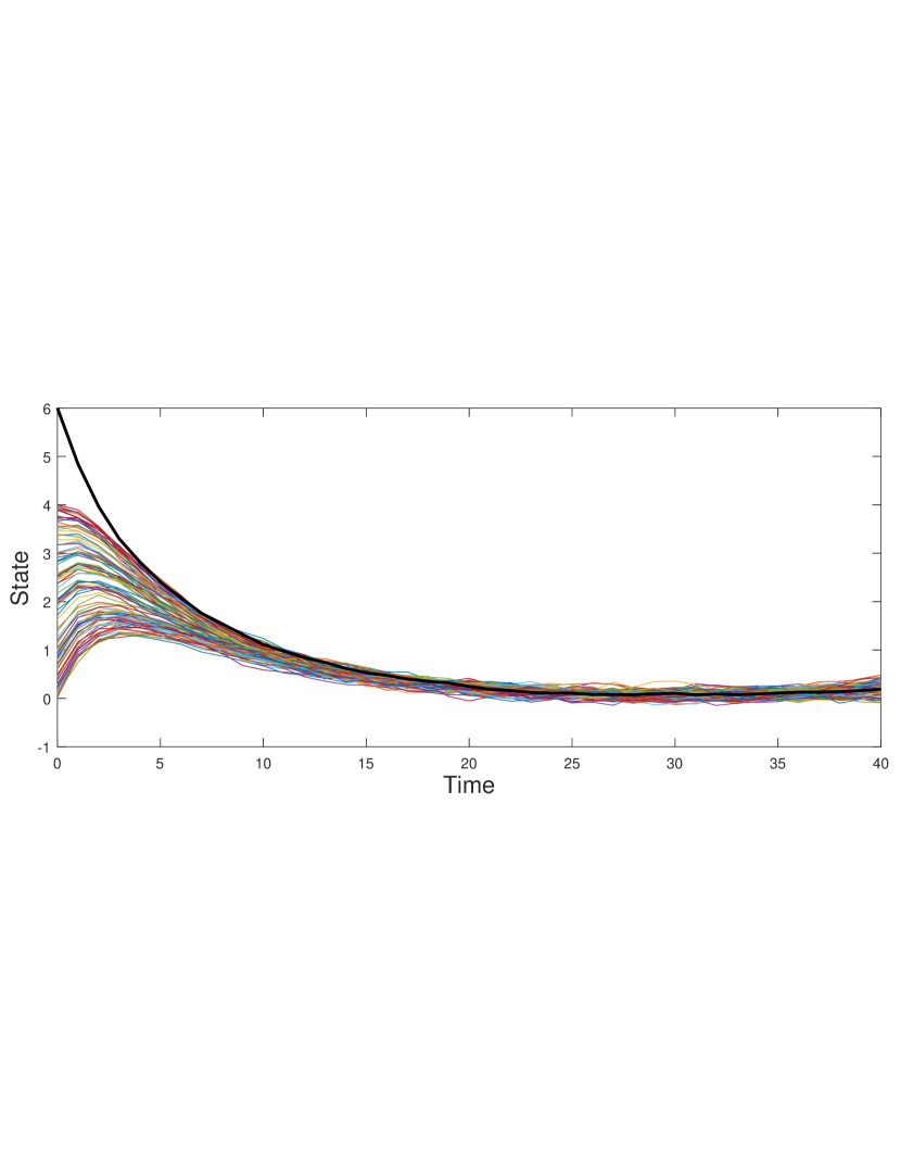
Figure 1: Trajectories of the leader and $100$ randomly selected followers in Example 1.

The next example demonstrates the efficacy of the results obtained in this work, for the special case of leaderless multi-agent networks.

Example 2: Consider a multi-agent system consisting of $100$ agents that are to track a constant reference trajectory $x^{0}_{1}=3$. The following parameters are used in the simulation:

$$A^{0}_{t}=1,\quad B^{0}_{t}=0,\quad D^{0}_{t}=0,\quad A_{t}=1,\quad B_{t}=0.5,$$ (106)

$$D_{t}=0.05,\quad E_{t}=0,\quad Q^{0}_{t}=0,\quad R^{0}_{t}=0,$$ (107)

$$Q_{t}=0.1,\quad P_{t}=20,\quad R_{t}=100,\quad H_{t}=0.5,\quad F_{t}=60,$$ (108)

$$T=40,\quad w^{i}_{t}\sim\mathcal{N}(0,0.02)\quad\forall i\in\mathbb{N}_{100}.$$ (109)

Similar to Example 1, each follower computes its control action according to (18). It is to be noted that in the leaderless case, the agents do not communicate as discussed in Remark 3.

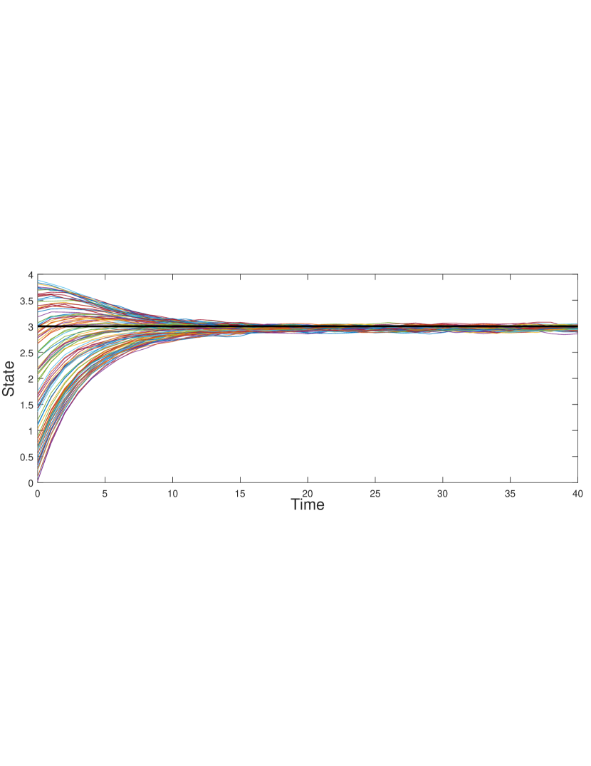
Figure 2: Trajectories of the followers in Example 2.

The results are given in Figure 2, analogously to Figure 1, and show that consensus is achieved as the states of all followers converge to the same value.

V Conclusions

A mean-field approach to the decentralized control of a leader-follower multi-agent network with a single leader is presented in this paper, where the states of the leader and followers are coupled in the dynamics and cost. A near-optimal strategy for a non-classical information structure is proposed such that the strategy is obtained by solving two decoupled Riccati equations, where the dimension of the matrices in these equations is independent of the number of followers. This means that the proposed method is not only distributed, it is also scalable. It is shown that the proposed solution converges to the optimal strategy at a rate inversely proportional to the number of followers. The effectiveness of the results is verified by simulation, for two different multi-agent settings with 1000 and 100 followers.

As suggestions for future research directions, one can extend the results to the case of infinite horizon, multiple leaders, heterogeneous followers, and weighted cost functions, under standard assumptions in mean-field teams [14]. The approach is robust in the sense that the failure of a small number of followers has negligible impact on the mean-field for a network of sufficiently large population.

References

• [1] J. A. Fax and R. M. Murray, “Information flow and cooperative control of vehicle formations,” IEEE Transactions on Automatic Control, vol. 49, no. 9, pp. 1465–1476, 2004.
• [2] P. Rawat, K. D. Singh, H. Chaouchi, and J. M. Bonnin, “Wireless sensor networks: a survey on recent developments and potential synergies,” Supercomputing, vol. 68, no. 1-48, 2014.
• [3] L. Gupta, R. Jain, and G. Vaszkun, “Survey of important issues in UAV communication networks,” IEEE Communications Surveys & Tutorials, vol. 18, no. 2, pp. 1123–1152, 2016.
• [4] C. W. Reynolds, “Flocks, herds and schools: A distributed behavioral model,” SIGGRAPH Comput. Graph., vol. 21, no. 4, pp. 25–34, 1987.
• [5] R. Olfati-Saber, “Flocking for multi-agent dynamic systems: algorithms and theory,” IEEE Transactions on Automatic Control, vol. 51, no. 3, pp. 401–420, 2006.
• [6] A. Jadbabaie, J. Lin, and A. S. Morse, “Coordination of groups of mobile autonomous agents using nearest neighbor rules,” IEEE Transactions on Automatic Control, vol. 48, no. 6, pp. 988–1001, 2003.
• [7] W. Ren, R. W. Beard, and E. M. Atkins, “Information consensus in multivehicle cooperative control,” IEEE Control Systems, vol. 27, no. 2, pp. 71–82, 2007.
• [8] R. Olfati-Saber, J. A. Fax, and R. M. Murray, “Consensus and cooperation in networked multi-agent systems,” Proceedings of the IEEE, vol. 95, no. 1, pp. 215–233, 2007.
• [9] P. E. Caines, Linear stochastic systems.   John Wiley and Sons, Inc., 1987.
• [10] H. Witsenhausen, “A counterexample in stochastic optimum control,” SIAM Journal on Control and Optimization, vol. 6, pp. 131–147, 1968.
• [11] K. H. Movric and F. L. Lewis, “Cooperative optimal control for multi-agent systems on directed graph topologies,” IEEE Transactions on Automatic Control, vol. 59, no. 3, pp. 769–774, 2014.
• [12] Y. Cao and W. Ren, “Optimal linear-consensus algorithms: An LQR perspective,” IEEE Transactions on Systems, Man, and Cybernetics, Part B (Cybernetics), vol. 40, no. 3, pp. 819–830, 2010.
• [13] F. Borrelli and T. Keviczky, “Distributed LQR design for identical dynamically decoupled systems,” IEEE Transactions on Automatic Control, vol. 53, no. 8, pp. 1901–1912, 2008.
• [14] J. Arabneydi, “New concepts in team theory: Mean field teams and reinforcement learning,” Ph.D. dissertation, Dep. of Electrical and Computer Engineering, McGill University, Montreal, Canada, 2016.
• [15] J. Arabneydi, M. Baharloo, and A. G. Aghdam, “Optimal distributed control for leader-follower networks: A scalable design,” in Proceedings of the \nth31 IEEE Canadian Conference on Electrical and Computer Engineering, 2018, pp. 1–4.
• [16] J. Arabneydi and A. G. Aghdam, “A certainty equivalence result in team-optimal control of mean-field coupled Markov chains,” in Proceedings of the \nth56 IEEE Conference on Decision and Control, 2017, pp. 3125–3130.
• [17] ——, “Optimal dynamic pricing for binary demands in smart grids: A fair and privacy-preserving strategy,” in Proceedings of American Control Conference, 2018, pp. 5368–5373.
• [18] J. Arabneydi and A. Mahajan, “Team-optimal solution of finite number of mean-field coupled LQG subsystems,” in Proceedings of the \nth54 IEEE Conference on Decision and Control, 2015, pp. 5308 – 5313.