Optimal Distributed Control for Leader-Follower Networks: A Scalable Design

Abstract

The focus of this paper is directed towards optimal control of multi-agent systems consisting of one leader and a number of followers in the presence of noise. The dynamics of every agent is assumed to be linear, and the performance index is a quadratic function of the states and actions of the leader and followers. The leader and followers are coupled in both dynamics and cost. The state of the leader and the average of the states of all followers (called mean-field) are common information and known to all agents; however, the local state of the followers are private information and unknown to other agents. It is shown that the optimal distributed control strategy is linear time-varying, and its computational complexity is independent of the number of followers. This strategy can be computed in a distributed manner, where the leader needs to solve one Riccati equation to determine its optimal strategy while each follower needs to solve two Riccati equations to obtain its optimal strategy. This result is subsequently extended to the case of the infinite horizon discounted and undiscounted cost functions, where the optimal distributed strategy is shown to be stationary. A numerical example with $100$ followers is provided to demonstrate the efficacy of the results.

Proceedings of IEEE Canadian Conf. on Elec. and Comp. Eng., 2018.

I Introduction

There has been a growing interest in networked control systems in recent years, due to their applications in emerging areas such as control of a platoon of autonomous vehicles, environmental monitoring using sensor networks, and surveillance using a team of UAVs [1, 2, 3]. In particular, in the control of multi-agent systems, every agent exchanges some information with a subset of agents in order to properly coordinate its position and movement such that a global objective is achieved. To this end, each agent requires some computational effort in order to compute its control action based on the information available to it.

The leader-follower structure is particularly very common in the coordination control of multi-agent networks. In this type of system, each agent is either a leader or a follower, where the movement of the followers is dependent on the trajectory of the leader(s). A global objective that is of special interest is consensus, where the states of the agents are desired to converge to a common value [4, 5, 6]. If the communication graph of the network is connected, then consensus can be reached using a linear strategy. However, such strategy suffers from the curse of dimensionality, in general. In addition, the required amount of communication between agents under this type of strategy is typically high. This can lead to some practical problems, specially given that the battery consumption of each node is closely related to the amount of its required communication. An optimal control strategy can therefore be very important for the efficient use of resources in the network. Inspired by this objective, the authors in [7, 8] study distributed linear quadratic control. Although the above techniques are effective in many cooperative control applications, they are limited by the computational cost, making them unsuitable for large-scale networks. A large-scale network of homogeneous agents with decoupled dynamics is investigated in [9], for which the infinite-horizon optimal control strategy is obtained by solving two scalable coupled algebraic Riccati equations.

The present work aims to address the above shortcomings for a leader-follower multi-agent network with a large number of followers. It is assumed that the graph representing the network is such that the average of the states of the followers and the local state of the leader are available to every agent. In contrast to [9], the network considered in this paper has a leader, the dynamics of agents are coupled, and the cost function can be either finite-horizon or infinite-horizon. The mean-field team approach [10] is used in this paper to obtain the optimal control strategy by solving two scalable decoupled Riccati equations.

This paper is organized as follows. In Section II, a leader-follower multi-agent network with the mean-field information structure is formulated. The main result of the paper is developed in Section III for the finite-horizon cost function, and is then extended to the infinite-horizon case in Section IV. Simulation results are provided in Section V, and the paper is concluded in Section VI.

II Problem Formulation

In this paper, $\mathbb{N}$ and $\mathbb{R}$ represent natural and real numbers, respectively, and given any $k\in\mathbb{N}$, the finite set of integers $\{1,2,\ldots,k\}$ is denoted by $\mathbb{N}_{k}$.

Consider a multi-agent network with one leader and $n\in\mathbb{N}$ followers, operating over a finite control horizon $T\in\mathbb{N}$. Let $x^{i}_{t}\in\mathbb{R}^{d_{x}}$ and $u^{i}_{t}\in\mathbb{R}^{d_{u}},$ $d_{x},d_{u}\in\mathbb{N}$, denote the state and action of follower $i\in\mathbb{N}_{n}$ at time $t\in\mathbb{N}_{T}$, respectively. Denote the average of the states of the followers at time $t$ by

$$\bar{x}_{t}=\frac{1}{n}\sum_{i=1}^{n}x^{i}_{t}.$$

Following the terminology of mean-field teams [10], we refer to the average of the states of the followers as mean-field in the sequel. Let also $x^{0}_{t}\in\mathbb{R}^{d_{x}}$ and $u^{0}_{t}\in\mathbb{R}^{d_{u}}$ denote the state and action of the leader at time $t\in\mathbb{N}_{T}$, respectively. The dynamics of the leader at time $\mathbb{N}_{T}$ is given by

$$x^{0}_{t+1}=A^{0}_{t}x^{0}_{t}+B^{0}_{t}u^{0}_{t}+D^{0}_{t}\bar{x}_{t}+w^{0}_{t},$$ (1)

where $w^{0}_{t}\in\mathbb{R}^{d_{x}}$ is the state noise of the leader. Similarly, the dynamics of follower $i\in\mathbb{N}_{n}$ is described by

$$x^{i}_{t+1}=A_{t}x^{i}_{t}+B_{t}u^{i}_{t}+D_{t}\bar{x}_{t}+E_{t}x^{0}_{t}+w^{i}_{t},$$ (2)

where $w^{i}_{t}\in\mathbb{R}^{d_{x}}$ is the state noise of the $i$-th follower. In general, the leader’s dynamics may depend on the states of the followers. Similarly, the followers’ dynamics may depend on the state of the leader as well as the states of followers.

At each time $t\in\mathbb{N}_{T}$, the leader observes its local state and the mean-field, i.e.,

$$u^{0}_{t}=g^{0}_{t}(x^{0}_{t},\bar{x}_{t}),$$ (3)

where $g^{0}_{t}:(\mathbb{R}^{d_{x}})^{2}\rightarrow\mathbb{R}^{d_{u}}$. Furthermore, each follower $i\in\mathbb{N}_{n}$ observes its local state, the state of the leader, and the mean-field, i.e.,

$$u^{i}_{t}=g^{i}_{t}(x^{i}_{t},\bar{x}_{t},x^{0}_{t}),$$ (4)

where $g^{i}_{t}:(\mathbb{R}^{d_{x}})^{3}\rightarrow\mathbb{R}^{d_{u}}$. Under this information structure, the privacy of each follower is preserved, i.e., the local state of each follower is only known to itself. Note that there are different ways to share the mean-field $\bar{x}_{t}$ among the agents, depending on the structure of the communication graph. For example, all agents can send their states to the leader and then the leader computes the mean and sends it back to every follower (in which case, a link is required between the leader and every follower). Alternatively, each agent can run a consensus algorithm to compute the mean-field within the control time interval.

It is desired that the leader and followers minimize a prescribed quadratic cost function, while achieving a global objective (such as consensus) as a group. This cost function can, for instance, reflect the coordination error of the agents as well as the energy consumption of the actuators, collectively. To this end, consider the following optimization problem.

Problem 1.

Given the dynamics (1) and (2) as well as the information structures (3) and (4), find the optimal strategy that minimizes the following performance index:

$$J_{T}=\mathbb{E}\Big{[}\sum_{t=1}^{T}(x^{0}_{t})^{\intercal}Q^{0}_{t}x^{0}_{t}+(u^{0}_{t})^{\intercal}R^{0}_{t}u^{0}_{t}\\ +\frac{1}{n}\sum_{i=1}^{n}(x^{i}_{t})^{\intercal}Q_{t}x^{i}_{t}+(x^{i}_{t}-x^{0}_{t})^{\intercal}P_{t}(x^{i}_{t}-x^{0}_{t})+(u^{i}_{t})^{\intercal}R_{t}u^{i}_{t}\\ +\frac{1}{2n^{2}}\sum_{i=1}^{n}\sum_{j=1}^{n}(x^{i}_{t}-x^{j}_{t})^{\intercal}H_{t}(x^{i}_{t}-x^{j}_{t})\Big{]},$$ (5)

where matrices $Q^{0}_{t},R^{0}_{t},Q_{t},P_{t},R_{t},$ and $H_{t}$ are symmetric.

Note that the rate of convergence of the followers to the leader is directly dependent on matrix $P_{t}$ in (5). Similarly, the movement of the followers as a group depends on matrix $H_{t}$.

Remark 1.

In the special case when matrices $B^{0}_{t}$, $D^{0}_{t}$, $Q^{0}_{t},$ and $R^{0}_{t}$ are zero, Problem 1 becomes the optimal control of a leaderless multi-agent system, where it is desired that the followers track the reference signal $x^{0}_{t}$.

In general, Problem 1 is difficult to solve due to its complex information structure. Since neither the information structure is partially nested [11] nor the problem is quadratic invariant [12], and in addition the noise processes are not necessarily Gaussian, one can not assume that the optimal strategy is linear. Moreover, the dimension of the augmented matrices, which are fully dense, increases with the number of followers, i.e., solving Problem 1 using existing techniques can be computationally expensive for a large number of followers.

III Main Result

In this section, the main result of this paper is presented. It is assumed that the primitive random variables satisfy the following standard assumption.

Assumption 1.

The initial states and noise processes are mutually independent in time.

At any time $t\in\mathbb{N}_{T}$, define the following matrices:

$$\bar{A}_{t}:=\left[\begin{array}[]{cc}A^{0}_{t}&D^{0}_{t}\\ E_{t}&A_{t}+D_{t}\end{array}\right],\bar{B}_{t}:=\left[\begin{array}[]{cc}B^{0}_{t}&0_{d_{x}\times d_{u}}\\ 0_{d_{x}\times d_{u}}&B_{t}\end{array}\right],$$ (6)

$$\bar{Q}_{t}:=\left[\begin{array}[]{cc}Q^{0}_{t}+P_{t}&-P_{t}\\ -P_{t}&Q_{t}+P_{t}\end{array}\right],\bar{R}_{t}:=\left[\begin{array}[]{cc}R^{0}_{t}&0_{d_{u}\times d_{u}}\\ 0_{d_{u}\times d_{u}}&R_{t}\end{array}\right].$$ (7)

Assumption 2.

Matrices $Q_{t}+P_{t}+H_{t}$ and $\bar{Q}_{t}$ are positive semi-definite and matrices $R^{0}_{t}$ and $R_{t}$ are positive definite.

For any $t\in\mathbb{N}_{T}$, define the following Riccati equation:

$$\breve{M}_{t}=-A_{t}^{\intercal}\breve{M}_{t+1}B_{t}\left(B_{t}^{\intercal}\breve{M}_{t+1}B_{t}+R_{t}\right)^{-1}B_{t}^{\intercal}\breve{M}_{t+1}A_{t}\\ +A_{t}^{\intercal}\breve{M}_{t+1}A_{t}+Q_{t}+P_{t}+H_{t},$$ (8)

where $\breve{M}_{T+1}=0_{d_{x}\times d_{x}}$. Define also the following Riccati equation:

$$\bar{M}_{t}=-\bar{A}_{t}^{\intercal}\bar{M}_{t+1}\bar{B}_{t}\left(\bar{B}_{t}^{\intercal}\bar{M}_{t+1}\bar{B}_{t}+\bar{R}_{t}\right)^{-1}\bar{B}_{t}^{\intercal}\bar{M}_{t+1}\bar{A}_{t}\\ +\bar{A}_{t}^{\intercal}\bar{M}_{t+1}\bar{A}_{t}+\bar{Q}_{t},$$ (9)

for any $t\in\mathbb{N}_{T}$, with $\bar{M}_{T+1}=\left[\begin{array}[]{cc}0_{d_{x}\times d_{x}}&0_{d_{x}\times d_{x}}\\ 0_{d_{x}\times d_{x}}&0_{d_{x}\times d_{x}}\end{array}\right]$.

Theorem 1.

Let Assumptions 1 and 2 hold. The optimal strategy for Problem 1 is linear and unique, i.e.,

$${u^{0}_{t}} =\bar{L}^{1,1}_{t}x^{0}_{t}+\bar{L}^{1,2}_{t}\bar{x}_{t},$$

$${u^{i}_{t}} =\breve{L}_{t}x^{i}_{t}+\bar{L}_{t}^{2,1}x^{0}_{t}+(\bar{L}_{t}^{2,2}-\breve{L}_{t})\bar{x}_{t},$$ (10)

where the gains $\{\breve{L}_{t},\bar{L}_{t}\}_{t=1}^{T-1}$ are obtained by solving Riccati equations (8) and (9) as follows:

$$\breve{L}_{t} =-\left(B_{t}^{\intercal}\breve{M}_{t+1}B_{t}+R_{t}\right)^{-1}B_{t}^{\intercal}\breve{M}_{t+1}A_{t},$$

$$\bar{L}_{t} =\left[\begin{array}[]{cc}\bar{L}^{1,1}_{t}&\bar{L}^{1,2}_{t}\\ \bar{L}^{2,1}_{t}&\bar{L}^{2,2}_{t}\end{array}\right]=-\left(\bar{B}_{t}^{\intercal}\bar{M}_{t+1}\bar{B}_{t}+\bar{R}_{t}\right)^{-1}\bar{B}_{t}^{\intercal}\bar{M}_{t+1}\bar{A}_{t}.$$ (13)

Proof.

Suppose every agent knows the centralized information $\{x^{0}_{t},x^{1}_{t},\ldots,x^{n}_{t}\}$. Let $\bar{u}_{t}=\frac{1}{n}\sum_{i=1}^{n}u^{i}_{t}$ and $\bar{w}_{t}=\frac{1}{n}\sum_{i=1}^{n}w^{i}_{t}$. We first transform the problem by using an isomorphic transformation and solve the transformed problem. Then, we use the inverse transformation to transform the obtained solution to the solution of the original problem, and show that the resultant (centralized) solution is implementable under the decentralized information structure. Define $\breve{x}^{i}_{t}:=x^{i}_{t}-\bar{x}_{t}$, $\breve{u}^{i}_{t}:=u^{i}_{t}-\bar{u}_{t}$, and $\breve{w}^{i}_{t}:=w^{i}_{t}-\bar{w}_{t}$. From (1) and (2),

$$\breve{x}^{i}_{t+1} =A_{t}\breve{x}^{i}_{t}+B_{t}\breve{u}^{i}_{t}+\breve{w}^{i}_{t},$$

$$\left[\begin{array}[]{c}x^{0}_{t+1}\\ \bar{x}_{t+1}\end{array}\right] =\bar{A}_{t}\left[\begin{array}[]{c}x^{0}_{t}\\ \bar{x}_{t}\end{array}\right]+\bar{B}_{t}\left[\begin{array}[]{c}u^{0}_{t}\\ \bar{u}_{t}\end{array}\right]+\left[\begin{array}[]{c}w^{0}_{t}\\ \bar{w}_{t}\end{array}\right].$$ (22)

Rewrite the cost function $J_{T}$, given by  (5), in terms of the new variables as follows:

$$J_{T}=\mathbb{E}\Big{[}\sum_{t=1}^{T}(x^{0}_{t})^{\intercal}Q^{0}_{t}x^{0}_{t}+(u^{0}_{t})^{\intercal}R^{0}_{t}u^{0}_{t}+\frac{1}{n}\sum_{i=1}^{n}(\breve{x}^{i}_{t}+\bar{x}_{t})^{\intercal}Q_{t}(\breve{x}^{i}_{t}+\bar{x}_{t})\\ +\frac{1}{n}\sum_{i=1}^{n}(\breve{x}^{i}_{t}+\bar{x}_{t}-x^{0}_{t})^{\intercal}P_{t}(\breve{x}^{i}_{t}+\bar{x}_{t}-x^{0}_{t})+(\breve{u}^{i}_{t}+\bar{u}_{t})^{\intercal}R_{t}(\breve{u}^{i}_{t}+\bar{u}_{t})\\ +\frac{1}{2n^{2}}\sum_{i=1}^{n}\sum_{j=1}^{n}(\breve{x}^{i}_{t}-\breve{x}^{j}_{t})^{\intercal}H_{t}(\breve{x}^{i}_{t}-\breve{x}^{j}_{t})\Big{]}.$$ (23)

The above relation can be simplified by exploiting the fact that $\frac{1}{n}\sum_{i=1}^{n}\breve{x}^{i}_{t}=0_{d_{x}\times 1}$ and $\frac{1}{n}\sum_{i=1}^{n}\breve{u}^{i}_{t}=0_{d_{u}\times 1}$. This leads to the following simplified equation:

$$J_{T}=\mathbb{E}\Big{[}\sum_{t=1}^{T}\left[\begin{array}[]{c}x^{0}_{t}\\ \bar{x}_{t}\end{array}\right]^{\intercal}\bar{Q}_{t}\left[\begin{array}[]{c}x^{0}_{t}\\ \bar{x}_{t}\end{array}\right]+\left[\begin{array}[]{c}u^{0}_{t}\\ \bar{u}_{t}\end{array}\right]^{\intercal}\bar{R}_{t}\left[\begin{array}[]{c}u^{0}_{t}\\ \bar{u}_{t}\end{array}\right]$$ (32)

$$+\frac{1}{n}\sum_{i=1}^{n}(\breve{x}^{i}_{t})^{\intercal}(Q_{t}+P_{t}+H_{t})(\breve{x}^{i}_{t})+(\breve{u}^{i}_{t})^{\intercal}R_{t}(\breve{u}^{i}_{t})\Big{]}.$$ (33)

The cost function $J_{T}$ in (32) is the sum of the cost functions of $n$ systems with state and action $(\breve{x}^{i}_{t},\breve{u}^{i}_{t})$, $i\in\mathbb{N}_{n},$ and one system with the state and action $(\{x^{0}_{t},\bar{x}_{t}\},\{u^{0}_{t},\bar{u}_{t}\})$. These $n+1$ systems are decoupled due to the certainty equivalence theorem [14]. As a result, $J_{T}$ is minimized when the cost functions of the $n+1$ systems with decoupled dynamics and cost are minimized, i.e.,

$$\left[\begin{array}[]{c}u^{0}_{t}\\ \bar{u}_{t}\end{array}\right]=\bar{L}_{t}\left[\begin{array}[]{c}x^{0}_{t}\\ \bar{x}_{t}\end{array}\right]\quad\text{and}\quad\breve{u}^{i}_{t}=\breve{L}_{t}\breve{x}^{i}_{t},\quad i\in\mathbb{N}_{n}.$$ (34)

We now transform the above solution to the solution of the original problem:

$$u^{i}_{t}=\breve{u}^{i}_{t}+\bar{u}_{t}=\breve{L}_{t}(x^{i}_{t}-\bar{x}_{t})+[\bar{L}^{2,1}_{t}\quad\bar{L}^{2,2}_{t}]\left[\begin{array}[]{c}x^{0}_{t}\\ \bar{x}_{t}\end{array}\right].$$ (35)

The transformed solution is optimal for the original decentralized problem because it is implementable under the information structure in Section II. ∎

According to Theorem 1, the leader must solve the Riccati equation (9) to determine its optimal strategy ($\bar{L}^{1,1}_{t}$, $\bar{L}^{1,2}_{t}$) whereas each follower must solve the Riccati equations (8) and (9) to find its optimal strategy ($\breve{L}_{t},\bar{L}^{2,1}_{t},$ $\bar{L}^{2,2}_{t}$): one for the local adjustment with their average (i.e., mean-field) and one for the global adjustment with the leader.

Corollary 1.

Let matrices $\breve{L}_{t}$ and $\bar{L}^{1,1}_{t}$ in Theorem 1 be invertible. The optimal strategy can be rewritten in the form of the solution of a standard consensus problem as follows:

$${u^{0}_{t}} =\sum_{i=1}^{n}\alpha_{t}(x^{0}_{t}-\beta_{t}x^{i}_{t}),$$

$${u^{i}_{t}} =\sum_{j=1}^{n}\gamma_{t}(x^{i}_{t}-\mu_{t}x^{j}_{t})+\sum_{i=1}^{n}\lambda_{t}(x^{0}_{t}-x^{i}_{t}),$$ (36)

where $\alpha_{t}=\frac{1}{n}\bar{L}^{1,1}_{t}$, $\beta_{t}=-(\bar{L}^{1,1}_{t})^{-1}\bar{L}^{1,2}_{t},\gamma_{t}=\frac{1}{n}\breve{L}_{t},\mu_{t}=-(\breve{L}_{t})^{-1}(\bar{L}^{2,2}_{t}+\bar{L}^{2,1}_{t}-\breve{L}_{t}),$ and $\lambda_{t}=\frac{1}{n}\bar{L}^{2,1}_{t}$.

Remark 2.

Corollary 1 provides the optimal information flow topology between the leader and followers for the case when such a topology is not pre-specified.

IV Infinite Horizon

In this section, the result of Theorem 1 is extended to the case of infinite horizon. To this end, it is assumed that the dynamics of the agents as well as the cost function are time-homogeneous; therefore, the subscript $t$ is omitted to simplify the notation. Given $\beta\in(0,1]$, define

$$J_{\infty}=\mathbb{E}\Bigg{[}\sum_{t=1}^{\infty}\beta^{t-1}\Big{(}(x^{0}_{t})^{\intercal}Q^{0}x^{0}_{t}+(u^{0}_{t})^{\intercal}R^{0}u^{0}_{t}\\ +\frac{1}{n}\sum_{i=1}^{n}(x^{i}_{t})^{\intercal}Qx^{i}_{t}+(x^{i}_{t}-x^{0}_{t})^{\intercal}P(x^{i}_{t}-x^{0}_{t})+(u^{i}_{t})^{\intercal}Ru^{i}_{t}\\ +\frac{1}{2n^{2}}\sum_{i=1}^{n}\sum_{j=1}^{n}(x^{i}_{t}-x^{j}_{t})^{\intercal}H(x^{i}_{t}-x^{j}_{t})\Big{)}\Bigg{]}.$$ (37)

When $\beta<1$, $J_{\infty}$ is called infinite-horizon discounted cost and when $\beta=1$, it is called infinite horizon undiscounted cost. The following standard assumption is imposed on the model.

Assumption 3.

Let $(\sqrt{\beta}A,\sqrt{\beta}B)$ and $(\sqrt{\beta}\bar{A},\sqrt{\beta}\bar{B})$ be stabilizable and $(\sqrt{\beta}A,Q^{1/2})$ and $(\sqrt{\beta}\bar{A},\bar{Q}^{1/2})$ be detectable.

Define the following two algebraic Riccati equations:

$$\breve{M}=-\beta A^{\intercal}\breve{M}B\left(B^{\intercal}\breve{M}B+\beta^{-1}R\right)^{-1}B^{\intercal}\breve{M}A\\ +\beta A^{\intercal}\breve{M}A+Q+P+H,$$ (38)

$$\bar{M}=-\beta\bar{A}^{\intercal}\bar{M}\bar{B}\left(\bar{B}^{\intercal}\bar{M}\bar{B}+\beta^{-1}\bar{R}\right)^{-1}\bar{B}^{\intercal}\bar{M}\bar{A}\\ +\beta\bar{A}^{\intercal}\bar{M}\bar{A}+\bar{Q}.$$ (39)

Theorem 2.

Let Assumptions 1, 2 and 3 hold. Then, the optimal control strategy is given by:

$${u^{0}_{t}} =\bar{L}^{1,1}x^{0}_{t}+\bar{L}^{1,2}\bar{x}_{t},$$ (40)

$${u^{i}_{t}} =\breve{L}x^{i}_{t}+\bar{L}^{2,1}x^{0}_{t}+(\bar{L}^{2,2}-\breve{L})\bar{x}_{t},$$ (41)

where the gains $\{\breve{L},\bar{L}\}$ are obtained by solving algebraic Riccati equations (38) and (39) as follows:

$$\breve{L} =-\left(B^{\intercal}\breve{M}B+\beta^{-1}R\right)^{-1}B^{\intercal}\breve{M}A,$$

$$\bar{L} =\left[\begin{array}[]{cc}\bar{L}^{1,1}&\bar{L}^{1,2}\\ \bar{L}^{2,1}&\bar{L}^{2,2}\end{array}\right]=-\left(\bar{B}^{\intercal}\bar{M}\bar{B}+\beta^{-1}\bar{R}\right)^{-1}\bar{B}^{\intercal}\bar{M}\bar{A}.$$ (44)

Proof.

By a simple change of variables, an infinite-horizon discounted cost problem with the 4-tuple $(A,B,Q,R)$ and discount factor $\beta$ can be transformed to an infinite-horizon undiscounted cost problem with 4-tuple $(\sqrt{\beta}A,\sqrt{\beta}B,Q,R)$. By applying the same isomorphic transformation as in the proof of Theorem 1 on the resultant undiscounted formulation, and using a similar argument as in that proof, the $n+1$ decoupled systems are obtained. ∎

V Numerical Example

Example 1. In this section, we present an example of a multi-agent system with a leader and $100$ followers to verify our theoretical results. Let the initial state of the leader be $30$, i.e., $x^{0}_{1}=30$, and the initial states of the followers be uniformly distributed random variables in the interval $[0,20]$. Let also the dynamics of the agents be driven by (1) and (2) with the following scalar parameters: $A^{0}_{t}=1,B^{0}_{t}=0.3,A_{t}=1,B_{t}=0.2,D^{0}_{t}=0.05,D_{t}=0.01,E_{t}=0.01,$ and noises:

$$w^{0}_{t}\sim\mathcal{N}(0,0.1),\quad w^{i}_{t}\sim\mathcal{N}(0,0.2),\quad\forall i\in\mathbb{N}_{n}.$$ (45)

Consider the cost function (5) with the following parameters:

$$Q^{0}_{t}=1,R^{0}_{t}=100,Q_{t}=0.1,P_{t}=50,R_{t}=50,H_{t}=1.$$ (46)

Assume first that $T=80$ (the finite-horizon case). Using Theorem 1, the optimal trajectories of the leader and followers shown in Figure 1 are obtained. Figure 1 shows that the states of the followers (thin colored curves) converge to a small neighborhood of the state of the leader (thick black curve). The size of this neighborhood depends, in fact, on the noise variance. In the special case when there is no noise, all followers’ states approach the state of the leader.

Assume now that $T=\infty$ (the infinite-horizon case with undiscounted cost). Using Theorem 2 in this case, the results demonstrated in Figure 2 are obtained, analogously to Figure 1. Figure 2 shows good convergence results for the followers in the presence of noise.

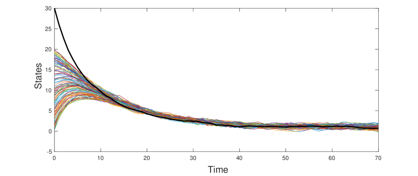
Figure 1: The trajectories of the leader and followers in Example 1 for the finite-horizon case.

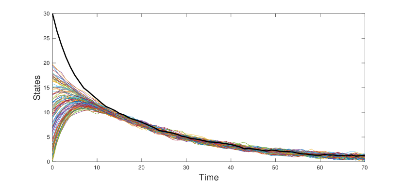
Figure 2: The trajectories of the leader and followers in Example 1 for the infinite-horizon case.

VI Conclusions

In this paper, optimal distributed control of a multi-agent system with a leader-follower structure is investigated. It is assumed that the average of the states of the followers and the local state of the leader are available to every agent. The optimal solution is obtained by solving two decoupled Riccati equations whose computational complexities are independent of the number of followers. In the infinite-horizon case, the Riccati difference equations become algebraic Riccati equations. As an interesting future work, one can consider the case where the number of followers is sufficiently large. In this case, the average of the states of followers can be efficiently approximated by the law of large numbers, which means that the only information to be shared is the local state of the leader. This implies that the communication topology of the network is described by a directed graph with paths from the leader to followers.

References

- [1] J. A. Fax and R. M. Murray, “Information flow and cooperative control of vehicle formations,” IEEE Transactions on Automatic Control, vol. 49, no. 9, pp. 1465–1476, 2004.
- [2] P. Rawat, K. D. Singh, H. Chaouchi, and J. M. Bonnin, “Wireless sensor networks: a survey on recent developments and potential synergies,” The Journal of supercomputing, vol. 68, no. 1, pp. 1–48, 2014.
- [3] L. Gupta, R. Jain, and G. Vaszkun, “Survey of important issues in uav communication networks,” IEEE Communications Surveys Tutorials, vol. 18, no. 2, pp. 1123–1152, 2016.
- [4] A. Jadbabaie, J. Lin, and A. S. Morse, “Coordination of groups of mobile autonomous agents using nearest neighbor rules,” IEEE Transactions on Automatic Control, vol. 48, no. 6, pp. 988–1001, 2003.
- [5] R. Olfati-Saber, J. A. Fax, and R. M. Murray, “Consensus and cooperation in networked multi-agent systems,” Proceedings of the IEEE, vol. 95, no. 1, pp. 215–233, 2007.
- [6] W. Ren, R. W. Beard, and E. M. Atkins, “Information consensus in multivehicle cooperative control,” IEEE Control Systems, vol. 27, no. 2, pp. 71–82, 2007.
- [7] K. H. Movric and F. L. Lewis, “Cooperative optimal control for multi-agent systems on directed graph topologies,” IEEE Transactions on Automatic Control, vol. 59, no. 3, pp. 769–774, 2014.
- [8] Y. Cao and W. Ren, “Optimal linear-consensus algorithms: An LQR perspective,” IEEE Transactions on Systems, Man, and Cybernetics, Part B (Cybernetics), vol. 40, no. 3, pp. 819–830, 2010.
- [9] F. Borrelli and T. Keviczky, “Distributed LQR design for identical dynamically decoupled systems,” IEEE Transactions on Automatic Control, vol. 53, no. 8, pp. 1901–1912, 2008.
- [10] J. Arabneydi, “New concepts in team theory: Mean field teams and reinforcement learning,” Ph.D. dissertation, McGill University, 2016.
- [11] Y. C. Ho and K. h. Chu, “Team decision theory and information structures in optimal control problems–part I,” IEEE Transactions on Automatic Control, vol. 17, no. 1, pp. 15–22, 1972.
- [12] M. Rotkowitz and S. Lall, “A characterization of convex problems in decentralized control,” IEEE Transactions on Automatic Control, vol. 51, no. 2, pp. 274–286, 2006.
- [13] H. Witsenhausen, “A counterexample in stochastic optimum control,” SIAM Journal Of Control And Optimization, vol. 6, pp. 131–147, 1968.
- [14] P. E. Caines, Linear stochastic systems. John Wiley and Sons, Inc., 1987.