NuSTAR Observations of Abell 2163: Constraints on Non-thermal Emission

Abstract

Since the first non-thermal reports of inverse Compton (IC) emission from the intracluster medium (ICM) of galaxy clusters at hard X-ray energies, we have yet to unambiguously confirm IC emission in observations with newer facilities. RXTE detected IC emission in one of the hottest known clusters, Abell 2163 (A2163), a massive merging cluster with a giant radio halo—the presumed source of relativistic electrons IC scattering CMB photons to X-ray energies. The cluster’s redshift ($z\sim 0.2$) allows its thermal and non-thermal radio emission to fit NuSTAR’s FOV, permitting a deep observation capable of confirming or ruling out the RXTE report. The IC flux provides constraints on the average magnetic field strength in a cluster. To determine the global diffuse IC emission in A2163, we fit its global NuSTAR spectrum with four models: single (1T) and two-temperature (2T), 1T+power law component (T$+$IC), and multi-temperature+power law (9T$+$IC). Each represent different characterizations of the thermal ICM emission, with power law components added to represent IC emission. We find the 3–30 keV spectrum can be described by purely thermal emission, with a global average temperature of $kT=(11.8\pm 0.2)$ keV. The IC flux is constrained to $<$4.0$\times$$10^{-12}$ erg s^-1 cm^-2 using the 1T$+$IC model and $<$1.6$\times$$10^{-12}$ erg s^-1 cm^-2 with the more physical 9T$+$IC model, both to 90$\%$ confidence levels. Combining these limits with 1.4 GHz diffuse radio data from the VLA, we find the average magnetic field strength to be $>$$0.22\mu$G and $>$$0.35\mu$G, respectively, providing the strongest constraints on these values in A2163 to date.

1 Introduction

Galaxy clusters are the largest form of gravitationally bound objects known in the Universe, reaching masses of up to $\sim$$10^{15}~{}M_{\odot}$. Due to the presence of a deep gravitational potential well, the gas or intracluster medium (ICM) heats up to temperatures between $10^{7-8}$ K, or equivalently, $kT\sim 1$–10 keV, which provides pressure support to the gas against gravitational collapse. The temperature and density of the cluster can be used to calculate the pressure profile, which in turn can be used to determine the mass under the assumption of hydrostatic equilibrium (e.g., Bahcall & Cen, 1993; Vikhlinin et al., 2009; Ettori et al., 2019).

When two clusters undergo a merger event, the gas is heated by shock fronts and mixed by turbulence, bringing it to a new virial temperature. Merging clusters also host diffuse radio synchrotron emission (radio halos and relics) that require a non-thermal electron population presumably made visible by some kind of Fermi-like acceleration process related to the merger (Giovannini et al., 1999). Surveys by Rossetti et al. (2016) show that nearly one half of all known galaxy clusters are undergoing a merger event. The same accelerated relativistic electrons radiating synchrotron emission in the radio must produce non-thermal emission in the form of inverse Compton (IC) scattering through interactions with cosmic microwave background (CMB) photons.

Abell 2163 (hereafter, A2163) is one of the most massive clusters observed in the Universe (Markevitch et al., 1994). It is also one of the most distant and rich clusters within the Abell catalogue (Abell, 1958; Markevitch et al., 1996). The cluster is currently undergoing a merger event (Maurogordato et al., 2008). Original temperature measurements suggested a global temperature of 15 keV (Arnaud, 1992). Past X-ray surveys have shown the gas distribution within the cluster to be non-isothermal, including an evident temperature gradient within the core of the cluster (Markevitch et al., 1994, 1996). In later studies, the global temperature of the cluster has fallen to values between 12 keV and 13 keV (Hansen et al., 2002).

Claims have been made of non-thermal emission due to the inverse Compton scattering of CMB photons by the relativistic electrons present in the ICM within the cluster (Feretti et al., 2001; Rephaeli et al., 2006; Million & Allen, 2009; Ota et al., 2014). Data taken by Beppo-SAX failed to detect significant IC emission, yielding an upper limit on the flux of the IC scattering ($F_{NT}$) between 20-80 keV at 90% confidence level less than 5.6 $\times$ $10^{-12}$ erg s^-1 cm^-2 (Feretti et al., 2001). A long observation RXTE was argued to show a detection with large uncertainties of $F_{NT}$ $\sim$ $1.1^{+1.7}_{-0.7}$ $\times$ $10^{-11}$ erg s^-1 cm^-2 (Rephaeli et al., 2006), nearly 25% of the integrated 3-50 keV flux, inconsistent with the Beppo-SAX upper limit. Using Chandra, Million & Allen (2009) argue a detection of $F_{NT}$ $\sim$ $3.9^{+1.0}_{-1.0}$ $\times$ $10^{-12}$ erg s^-1 cm^-2 between 0.6-7.0 keV, which accounts for roughly 10% of the integrated flux. A later 90% upper limit of detection, $F_{NT}$ $<$ 1.2 $\times$ $10^{-11}$ erg s^-1 cm^-2 (Ota et al., 2014) was provided by work done using the Hard X-Ray Detector (HXD) on the Suzaku satellite in combination with XMM-Newton data.
Using IC upper limits in conjunction with radio data yields a lower limit on the magnetic field (Rephaeli, 1979). It is important to know the magnetic field strength of galaxy clusters because they play a role in energy distribution in the gas as well as contribute dynamically to physical processes occurring within clusters (Carilli & Taylor, 2002). Due to the large scale of clusters, knowing constraints on the magnetic field can also provide insight into cosmological magnetic fields and their evolution (Vacca et al., 2018).

In this paper, we present a deep NuSTAR (Nuclear Spectroscopic Telescope Array) (Harrison et al., 2013) observation of A2163 in order to detect or constrain IC emission. We also use data obtained from the VLA (Very Large Array) in the 1.4 GHz range to get constraints on the lower limit of the magnetic field strength. In Section 2, we discuss the observations and how the data was processed. In Section 3, we show how the background was modeled as well as discuss the individual components within this model. In Section 4, we describe our analytical approach on the data and which model provides the best constraints. In Section 5, we summarize our findings with respect to previous studies and discuss future possibilities. We also provide Appendix A) containing information regarding an issue with this observation concerning auxiliary response file generation. For this paper, all errors are quoted at the 90% confidence level.

2 Observations and Data Reduction

2.1 X-ray

A2163 was observed by NuSTAR for a net raw exposure time of 115 ks, including periods when the cluster was occulted by the Earth. The observation was carried out between March 23rd, 2016 and March 26th, 2016. To filter the data, we used standard pipeline processing from HEASoft version 6.22 and NuSTARDAS version 1.7.1. In order to obtain clean spectra for analysis, we needed to remove high background periods from the data since our measurement is most sensitive in the background-dominated regime. Normally, this is done by setting the STRICT and TENTACLE flags within the nupipeline processing. The STRICT mode identifies when the telescope passes through the South Atlantic Anomaly (SAA) by detecting high-gain shield single rates stored in the file for the SAA calculation algorithm. The TENTACLE flag detects time intervals in which the CZT detectors have an increase in event count rates when crossing the SAA. This filtering, however, can at times be too strict and remove good periods as well as miss high background periods. To combat this, we instead process the data with these flags turned off and derive a custom set of good time intervals (GTIs) manually. We create light curves using all the data from the instrument for the A and B telescopes separately by running the lcfilter command. These light curves are then binned in bins of 100 s. We manually identify and exclude time intervals where the count rate is above the local distribution of rates, which is carried out in three passes. The first pass is to eliminate high background periods due to the SAA at harder energies (50-160 keV). The second pass is again performed in the same energy range to further reduce smaller contributions from the SAA after the larger background intervals have been removed. The final pass is done in low energy ranges (1.6-20 keV) to remove high background periods due to solar activity. This process reduced the exposure time to 112 ks in both the A and B telescopes. After filtering the data based on our new set of good time intervals (GTIs), there were no notable fluctuations in the final light curve, suggesting a clean background (see Figure 1).

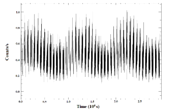
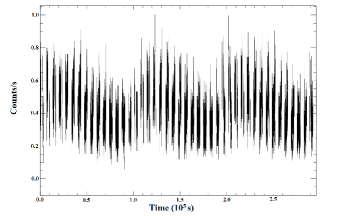
Figure 1: Filtered light curves for both the A (top) and B (bottom) telescopes following the process described in Section 2.1. The light curves have been filtered in the 50-160 keV energy range to eliminate SAA background contributions as well as the 1.6-20 keV range to remove solar activity background contributions.

Using the new GTIs, we reprocessed the data with nupipeline. The cleaned files were used to generate images with XSELECT. Exposure maps were created using nuexpomap. For spectral fitting, spectra, response matrices, and auxiliary response files (RMFs and ARFs, respectively) were initially made with nuproducts. Generally, nuproducts has a flag (extended = yes) that weights the ARF based on the distribution of events within the chosen extraction region. This is under the assumption that the observed spatial distribution of source photons is identical to the incident distribution of the source, which in principle is not entirely true. It appears that in the case of this particular observation, nuproducts produced ARFS are normalized using an incorrect weighting scheme.

To account for this issue, we calculate ARFs for a given region following the intended procedure of nuproducts, extended = yes, with a grid of point source effective area curves across the region summed and weighted by the relative number of net counts in that vicinity based on a background-subtracted image. We verify that this procedure reproduces similar results as point source ARFs created by nuproducts (see Appendix A for details). We present cleaned images of the cluster, along with the regions used in this analysis, in Figure 3.

2.2 Radio

We reanalyzed archival VLA data of A 2163 at 1.4 GHz (project AF328, same data used in Feretti et al. (2001)). The cluster was observed in C-array configuration for approximately 4 hours and twice in D configuration for a total of 3.4 hours. All observations used two intermediate frequency (IF) channels centered at 1365 MHz and 1435 MHz, with a bandwidth of 50 MHz/IF for the D configuration observations and 25 MHz/IF in C configuration.

We calibrated and reduced each dataset separately using the NRAO Astronomical Image Processing System (AIPS) package. We followed the standard calibration scheme, with amplitude and phase calibration carried out using the primary (3C286) and secondary (1557-000) calibration sources. The flux density scale was set using the Perley & Butler (2013) coefficients. We applied phase-only self-calibration to each dataset to reduce the effects of residual phase errors in the data. Final images were made using the multi-scale CLEAN algorithm implemented in the IMAGR task. After self-calibration, we combined the C- and D-configuration data into a single data set. A final cycle of phase-only self-calibration was applied to the combined dataset to improve the image quality. We reached an rms sensitivity level of 25 $\mu$Jy beam^-1 in the final combined image, with a restoring beam of $24^{\prime\prime}\times 18^{\prime\prime}$ (Figure 2).

We made images using only baselines longer than 0.5 k$\lambda$ and 1 k$\lambda$ to image respectively only the extended and compact radio sources unrelated to the diffuse radio halo. We identified 34 sources with a peak flux density above the 3$\sigma$ level of 0.075 mJy beam¹ within a region of $\sim$2 Mpc radius centered on the cluster X-ray centroid. These include the 3 tailed radio sources T1, T2 and T3 and 4 extended features (D1 to D4) with no obvious optical counterpart identified by Feretti et al. (2001). Finally, we then subtracted the CLEAN components associated with these sources (for a total of 161 mJy) from the $uv$ data and used the resulting data set to obtain images of the diffuse radio emission using the multi-scale CLEAN. An image restored with a $55^{\prime\prime}\times 39^{\prime\prime}$ beam is shown in Figure 2. The image noise is 30 $\mu$Jy beam^-1. The radio spectral index was estimated to be $\sim$ 1 (Feretti et al., 2004).

The total halo flux density, measured within the $3\sigma$ isocontour is $189\pm 10$ mJy, where the errors include the flux calibration uncertainty (3%), the image noise and the error due to the subtraction of the individual radio sources in the halo region computed following Cassano et al. (2013). Within our global extraction region, we measure a flux density of 90 mJy.

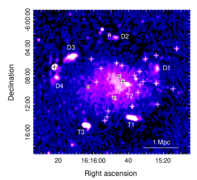
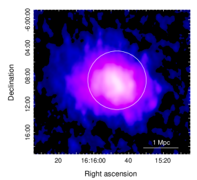
Figure 2: Radio images of A 2163 from the combined 1.4 GHz dataset. Top: radio brightness image before source subtraction. The angular resolution is $24^{\prime\prime}\times 18^{\prime\prime}$, in p.a. $-13^{\circ}$ and rms noise level is 25 $\mu$Jy beam^-1. Crosses mark the position of discrete radio sources. The tailed radio galaxies and peripheral diffuse sources identified by Feretti et al. (2001) are also labelled. Bottom: radio brightness image of the giant radio halo after source removal. The angular resolution is $55^{\prime\prime}\times 39^{\prime\prime}$, in p.a. $4^{\circ}$ and rms noise level is 30 $\mu$Jy beam^-1.

3 Background

One of the unique features of NuSTAR is the presence of a large open mast separating the focal plane and optics modules. This causes the observatory to be susceptible to stray light, producing a gradient across the FOV. The stray light-induced background must be separated from the instrumental background, which is generally spatially uniform, since it is produced by unknown cosmic background sources of variable intensity. We isolate these components with nuskybgd (Wik et al., 2014), which characterizes the background and allows background spectra and images to be generated.

3.1 Components

Since we have a good empirical understanding of the individual background components, we can characterize a background model from source free regions and apply the model to take into account the strengths of the background components within a source region. There are four main sources of background, each briefly detailed in this section. For a more detailed explanation see Wik et al. (2014).

The internal background of the instrument comes from a few different sources. The first is the radiation environment present in NuSTAR’s low earth orbit, which produces a flat background. Gamma rays that Compton scatter within the detector also produce background features. The rest of this component comes from fluorescence and activation lines mostly present within the range of 22-32 keV (Wik et al., 2014).

The next background component is the aperture stray light, which comes from unfocused X-rays that are able to pass through the aperture stops and strike the detectors due to NuSTAR’s open design. Because the CXB is roughly uniform throughout the sky but partially occulted by the optics bench, a gradient is produced across the FOV. The CXB spectral model used is the HEAO1 A2-determined model (Boldt, 1987) valid in the range from 3 keV to 60 keV.

Reflected and scattered stray light is also a source of background due to the open nature of the telescope. The backside of the aperture stops in particular are a prime source of reflection that is seen by the detectors. The three primary sources of light that gets reflected are the CXB, the Sun, and the Earth. About 10-20$\%$ of the unfocused light is reflected (Wik et al., 2014). Solar and terrestrial light are detected in lower energy bands, particularly around 1 keV during high periods of solar activity, accounting for roughly 40$\%$ of the events below 5 keV (Wik et al., 2014).

The final component is the focused cosmic background (fCXB), which is the background contribution from unresolved foreground and background sources within the field of view. Contributions from the fCXB are generally below 15 keV and amount to $\sim$10% of the CXB photons detected, with the majority entering undeflected through the aperture stops (Wik et al., 2014).

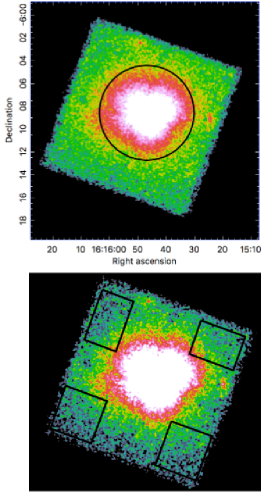
Figure 3: Top: A false color (faint to bright represented by black to blue to green to yellow to red to white) combined (A$+$B) log scaled image in the 4–25 keV band, smoothed by a Gaussian kernel with $\sigma$ = 3 pix, and stretched to show features in the outer parts of the FOV. The source region from which spectra are extracted is shown as the black circle. A foreground galaxy group lies in the north and a background AGN is located to the west of the cluster center were kept outside the extraction region to prevent false detections of non-thermal emission. Bottom: The nuskybgd regions used to characterize the background of the cluster.

3.2 Background Characterization

Due to the well understood nature of the aforementioned background components, we can model its composition by creating regions that are relatively source-free, as shown in the bottom panel of Figure 3. This, in combination with knowing how these components vary spatially, allows us to apply that to the source region. These source-free regions are not always completely source-free given the diffuse nature of the emission from the galaxy cluster. To take this into account, we produced a contamination file containing APEC models used to characterize potential thermal emission due to the cluster with the temperature thawed. Results for our background fits for both Telescopes A and B can be seen in Figure 4. We find that there is no major difference observed in the background between both telescopes.

3.3 Systematic Uncertainties

To include systematic uncertainties, we follow the procedure outlined in Wik et al. (2014) in their analysis of the Bullet Cluster. Due to the faint nature of an IC emission spectral component, it is paramount to accurately consider systematic uncertainties in order to prevent false detections and to derive conservative upper limits. For the instrumental background, we adopt a 90% uncertainty of roughly 3$\%$ to account for systematic variations. For the aperture CXB, we adopt a systematic uncertainty of 8$\%$. The origin of this value is from cosmic variance, which is when measurements are affected by the cosmic large-scale structure (i.e., variability in flux that depends on the solid angle sampled). The uncertainty in the fCXB is derived in the same way, considering the smaller solid angle sampled by these sources, yielding potential variations of 42%.

4 Analysis

Before extracting spectra from the data, we must first generate images of the cluster to see if there are any bright point sources within the FOV. The post-pipeline event files can produce images in any energy band by filtering the PHA column in xselect. In Figure 3, we present a smoothed image of the raw counts extracted from the combined A and B telescope cleaned event files in the 4–25 keV band. We then exposure-correct and background-subtract the images with exposure and background images generated from two routines: nuexpomap and nuskybgd. Exposure maps are created at single energies for each band corresponding to the mean emission weighted energy of the band assuming an APEC thermal model with $kT=$ 10 keV. Images in four different energy bands (top row: 3–8 keV and 8–15 keV; bottom row: 15–30 keV, 30–40 keV) are presented in Figure 5. From the 3–8 keV image, we see the brightest cluster emission, along with two other sources, located to the north (a foreground galaxy group unrelated to A2163) and west (a background AGN) of the cluster. These sources were avoided to reduce emission that may contaminate the data and be confused with the diffuse non-thermal emission we are searching for. From the 8–15 keV image, the northern group disappears because of its soft spectrum, while the harder AGN source to the west remains. Above 15 keV, the cluster’s emission begins to blend in with that of the background and above 30 keV the image becomes entirely background dominated. There are no appreciable features that may resemble non-thermal emission at these higher energies present. No other point sources are evident outside of the cluster, however due to NuSTAR’s large PSF it is difficult to rule out possible sources of contamination within the brightest region of diffuse cluster emission. The entire FOV of NuSTAR is a factor of two smaller than the effective PSF of Suzaku’s HXD-PIN and Swift-BAT instruments, which greatly reduces the chances of point sources (or a single bright AGN) contaminating the hard X-ray emission. Figure 3 shows the source region from which we extracted the spectra that will be discussed in the following subsections.

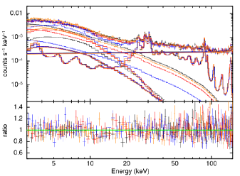
Figure 4: Fits to the background spectra extracted from the regions shown in Figure 3; the top and bottom panels show the spectra from Telescope A and B, respectively. The background at softer energies ($<$5 keV) is primarily due to the Sun, which is combined with the model that includes instrumental background lines present at all energies. Between 10–20 keV, the undeflected CXB through the aperture stops is dominant, while the portion focused through the optics (fCXB) is $\sim$10$\times$ fainter. The steeper spectral models in this energy range are due to ICM emission from the cluster. At harder energies, cosmic ray-induced activation and fluorescence lines dominate, along with a flat continuum component representing the overall instrumental background level.

4.1 Spectra

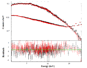
Figure 7: Upper panel: Background-subtracted global spectra of A2163 over the 3–30 keV bandpass fit to a single temperature (1T) APEC model (solid lines), with the data from Telescopes A and B shown in black and red, respectively. The lower curves show the background. Lower Panel: Residuals of the fit scaled by the uncertainty in each bin.

Spectra were generated with nuproducts from the region shown in Figure 3 and fit with XSPEC, with the fitted spectra shown in Figures 7, 8, 9, and 10. The two spectra from the A and B telescopes are generally consistent with each other. To include the impact of systematic uncertainties due to the background, we simulated 1000 different realizations of the individual components of the background described in section 3.1 randomly shifted by an amount consistent with the variances quoted in section 3.3, similar to the approach taken by Wik et al. (2014). The fluctuations are assumed to follow a Gaussian distribution. New background spectra are generated for each iteration, subtracted from the source spectra, which are grouped by 30 counts, and best-fit parameters are found using the modified Cash statistic (via the statistic cstat command in XSPEC). This was done to speed up the fitting process while also not creating an appreciable loss of information due to the larger bins (since the continuum components are of greatest interest).

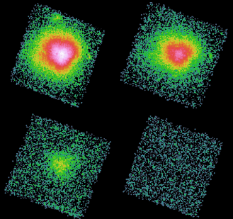
Figure 5: A2163 in different energy bands. Top left: 3–8 keV; top right: 8–15 keV; bottom left: 15–30 keV; bottom right: 30–40 keV. Each image has been background subtracted and exposure corrected. They are presented in a log scale from 0 counts s^-1 pix^-1 (in black) to 20+ counts s^-1 pix^-1 (in white) and smoothed by a Gaussian kernel with $\sigma$ = 3 pix. There are fewer cluster counts present in the higher energy images and there are no obvious morphological changes with respect to the lower energy images, which are dominated by thermal photons.

4.2 Models

In clusters with radio relics and radio halos like A2163, there must exist IC emission at some level. In the case where it is weak, such as with this cluster, the total model used to fit data becomes more important in differentiating non-thermal from thermal emission. Following the methodology done in Ota et al. (2014) for A2163 and Wik et al. (2014) for the Bullet Cluster, we use the four following models: single temperature (1T), two temperature (2T), single temperature added to a power law (T$+$IC), and multi-temperature added to a power law (9T$+$IC). The temperature components are all calculated using the APEC model within XSPEC. It should be noted that metal abundances are allowed to be free during the fitting process and that we ignore foreground absorption, due to NuSTAR’s lack of sensitivity below 3 keV. We verified that the latter has negligible affect on our results by multiplying all of our fits by the tbgas model, which takes as an input the Galactic absorption. Using values for $n_{H}$ of 0.118 (Kalberla et al., 2005) and 0.230 (based on results from Willingale et al. (2013), we found no statistically significant differences between the fits containing tbgas and those lacking it. All model parameters are discussed in more detail in the following subsections.

4.2.1 Single Temperature

The 1T model takes a very simplistic approach to characterizing the total emission from the cluster. If the gas is nearly isothermal and entirely thermal in nature, this model could provide a satisfactory fit given that NuSTAR’s 0.4 keV FWHM resolution limits our ability to separate the 6.7 keV He-like and 6.9 keV H-like iron lines—the only significant emission lines in NuSTAR’s bandpass at these temperatures. Previous work using XMM-Newton$+$Suzaku HXD-PIN data gave a best 1T model fit of $14^{+6}_{-5}$ keV (Ota et al., 2014). In contrast, our 1T fit to NuSTAR spectra results in $kT=11.8\pm 0.2$ keV (statistical uncertainty only), consistent with the previous estimate but much more precise. The C-stat value for this fit is 1434 with 1344 degrees of freedom (dof).

4.2.2 Two Temperature

Spatially-resolved temperature estimates from XMM-Newton, however, suggest that the gas within the ICM of A2163 is not isothermal (Govoni et al., 2004; Bourdin et al., 2011), consistent with ongoing merger activity. Despite previous such measurements, the true temperature structure of the cluster is unknown. Instead, these measurements provide emission-weighted temperatures potentially biased by a telescope’s effective area and gas projections along the line of sight. This means that the temperature is dependant on the energy range and calibration of the telescope. To better measure the temperature distribution detected by NuSTAR, a 2T model provides a way to take into account that NuSTAR is preferentially weighted towards hotter temperatures and may not agree with projected temperature structure measured at lower energies. Due to the lack of features in the thermal continua, a 2T model can in principle account for a range of temperatures.

We find the values for the two temperature components to be $T_{\rm h}=13.5^{+2.2}_{-1.1}$ and $T_{\rm l}=5.9^{+3.8}_{-3.1}$ keV. The C-stat value for this model is 1411 with 1342 dof, suggesting a better fit than the 1T model. If significant IC emission were detectable, it should be noticeable in this model through the hot temperature component, which would be unphysically high. If this is the case, then using a T+IC model would provide a better fit to the overall spectrum. As is the case with the 1T model, the thermal component would not entirely follow the actual thermal distribution, but the shape of the spectrum at higher energies would be better described by the non-thermal power law component.

4.2.3 T$+$IC

The T$+$IC model is a more accurate representation of the spectrum in the case when the non-thermal component is particularly prominent. In our limited bandpass, IC scattering follows a power law curve, so we use XSPEC’s power law model with a photon index of $\Gamma=2$, since our $\alpha$ value based on the radio data was $\sim$ 1, roughly following the best fit value found by Ota et al. (2014) of 2.18. We attempted to fit with a free photon index, but when done it would become unphysically steep. This is likely due to the photon index mimicking the effects of $T_{l}$ in the 2T model. It is important to note that due to declining counts at harder energies, a non-thermal component due to IC scattering needs to be strong enough to surmount worsening the fit at softer energies, where the majority of counts are located. Here, our thermal component and the power law normalization were left free. The best-fit temperature obtained from the model is $kT=11.4\pm 0.3$ keV, lower than just a single temperature model, which makes sense due to the harder non-thermal component accounting for some of the photons at the highest energies. The estimated power law flux from 20–80 keV for the T$+$IC model is $F_{\rm NT}$ $<$ 4.03 $\times$ $10^{-12}$ erg s^-1 cm^-2 with a 90$\%$ confidence level. We do not attempt a 2T+IC model, which in theory should better constrain the thermal components as mentioned before. This would provide a better constraint on a non-thermal excess at higher energies while minimizing the effects on the errors of the thermal parameters. However when doing this with A2163, one of the two thermal components gives a very low, unphysical temperature. Since this component is simply making small corrections to the model at the lowest energies, where uncertainties in the background or overall calibration are larger, the addition of a second temperature component provides no advantage over the T+IC model, which adequately accounts for the average thermal emission given the quality of the data. The C-stat value for this model is 1419 with 1343 dof, which means that this model does not fit the data as well as the 2T model. This signifies that the multi-temperature nature of the spectrum dominates over the need for a non-thermal component driven by an excess at hard energies.

4.2.4 Multi-temperature + IC

Given the spatially-resolved spread in temperatures in A2163, a model containing multiple temperature components and a non-thermal power law component should more accurately capture the emission at all X-ray energies. As found in the previous section, however, any model containing more than two free temperature components will become degenerate or unphysical. In this situation, a physically meaningful better fit will not be obtained due to the fewer degrees of freedom. To incorporate our knowledge of the true multi-temperature nature of A2163’s ICM, and to take advantage of NuSTAR’s spatial resolution, we extract spectra from 9 smaller regions within the global extraction region and fit them individually with single temperature models. We base these regions on those presented in the temperature map of Bourdin et al. (2011), which are shown in Figure 6, and the best-fit model parameters for each region are given in Table 1. When compared to the XMM-Newton temperature map, we do not observe the 18 keV, shock-like feature in the northeastern corner of the cluster (corresponding to our region 9). This difference is likely due to A2163’s placement with respect to the Galactic plane. The cluster lies close to the plane containing high amounts of neutral hydrogen. If the distribution of the column density varies on small angular scales, but is taken to be constant as done in the XMM-Newton study, the temperatures can be skewed to higher or lower values by the fit as the fit statistic at lower energies is more highly weighted than in the higher energy portions of the spectra. NuSTAR does not run into this issue due to its insensitivity to foreground absorption.

The resulting best-fit parameters are then used to construct a composite 9T thermal model that in principle better represents the thermal structure contained within the global spectrum. We combine this model with an IC component (9T$+$IC) twice, once keeping all the parameters that were found individually fixed other than the overall normalization and once allowing the temperatures to vary within their error range. The difference between these two methods was not significant, so we only report the former process. With the temperatures able to vary within their uncertainties, any weak non-thermal emission present that may bias the temperature estimate high in the single temperature fit is allowed to adjust in the fit to the global spectrum, where the IC component should be more significant. The normalization constant for this model was very close to one, meaning that the fit parameters were comparable to the parameters obtained when fitting the regions individually. Repeating the process for determining the non-thermal flux in the previous section, we obtain a flux of $F_{\rm NT}$ $<$ 1.64 $\times$ $10^{-12}$ erg s^-1 cm^-2. The C-stat value of this model is 1418 with 1345 dof, again suggesting that the best-fit model for the data is the 2T model.
It is possible that this method could have underestimated the presence of an IC component; i.e. the temperatures may be overestimated if hard IC emission is present, masquerading as hotter thermal flux in the model. In order to check for this possible bias, we ran a simulation test where we artificially inserted twice the amount of IC flux found in our upper limit, to check whether that level of IC emission would be missed by our approach or not. First, for each of our 9 regions, we create a 1T+IC model; the parameters of the thermal component are the same as those we found in our fits to the real data. The IC flux is added equally to each region, each with a photon index of 2 and a flux equal to two-ninths of our 90% upper limit. Spectra are simulated and then fit with a single temperature model. Following the procedure for the real data, we use the best-fit parameters from these single temperature fits to create a 9T model. We then add the 9 simulated spectra to create a global spectrum, which we fit with the 9T model plus a power law component in exactly the same way that we fit the real data with the 9T+IC model. Were IC emission being suppressed because it is being taken up by the thermal models, we should measure a lower IC flux from the global simulated spectrum than we included. However if the thermal models are not significantly biased by this level of underlying IC emission, then we should accurately measure the total amount of IC flux we added to the simulated spectra.
The temperatures measured of each simulated spectra were $\sim$0.2 keV higher than the true values with the exception of the cool core, which was about 2 keV higher. The global fit found an IC flux consistent with the injected flux detected at $3.9\sigma$ significance. Therefore we conclude that an IC flux at this level would have been detected with the detailed thermal modeling approach, and that the approach would not have led to a biased estimate of the flux. Since we estimate the presence of IC emission to be weaker and thus the temperatures estimated in individual regions to be less biased, the 9T+IC model provides an accurate and unbiased way to estimate the limit on the level of IC emission in A2163.

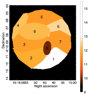
Figure 6: A temperature map inside the extraction region of our global spectra, consisting of 9 regions selected based on the work of Bourdin et al. (2011). We do not detect higher temperature gas in the northeast (in region 9) as seen in both Bourdin et al. (2011) and Ota et al. (2014). The discrepancy is likely due to spatially variable absorption, which NuSTAR is insensitive to. Temperature variations are primarily due to the disrupted cool core (region 8) and a region of hot gas likely heated by a shock front driven ahead of the cool core to the southwest (region 1). See Table 1 for temperatures, abundances, and normalizations.

Table 1: This table contains the individual temperatures and abundances measured within the 9 selected regions from our multi-temperature model. These regions were chosen loosely based on regions done in previous work to create a temperature map done by Bourdin et al. (2011).

	Temperature	Abundance	Norm
Region	(keV)	(Solar)	($10^{-3}$)
1	$15.55\pm 0.83$	$0.51\pm 0.21$	$1.41\pm 0.04$
2	$11.90\pm 0.32$	$0.37\pm 0.10$	$3.01\pm 0.05$
3	$11.67\pm 0.20$	$0.31\pm 0.06$	$7.74\pm 0.05$
4	$12.21\pm 0.78$	$0.22\pm 0.15$	$9.54\pm 0.04$
5	$11.67\pm 0.64$	$0.22\pm 0.14$	$1.53\pm 0.03$
6	$12.54\pm 0.51$	$0.19\pm 0.11$	$1.67\pm 0.07$
7	$11.65\pm 0.30$	$0.21\pm 0.08$	$3.23\pm 0.05$
8	$\phantom{0}9.95\pm 0.22$	$0.35\pm 0.06$	$2.44\pm 0.04$
9	$12.11\pm 0.20$	$0.30\pm 0.04$	$8.63\pm 0.07$

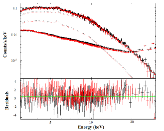
Figure 8: Fit of the global spectra to the two temperature model (2T: APEC$+$APEC model). Note how adding the second temperature component evens out the errant residuals around the Fe complex and at high energies, compared to the 1T model. Details are the same as in Fig. 7.

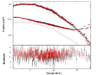
Figure 9: Fit of the global spectra to the single temperature plus power law model (T$+$IC: APEC$+$power law model). The two components are shown individually as dashed lines, with the thermal component’s contribution dominating over that of the IC component, which lies at or below the background level. Other details are the same as in Fig. 7.

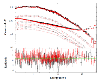
Figure 10: Fit of the global spectra to the nine temperature model plus power law (9T$+$IC: 9APEC$+$power law model, where each APEC model is fit using the parameters in Table 1. The lower dashed line is the non-thermal power law component, with all the dashed lines above it being brigher thermal components. Details are the same as in Fig. 7.

4.2.5 Preferred Model Including Systematic Uncertainties

Table 2: This table contains the results of our fits using the 1T, 2T, T$+$IC, and 9T$+$IC models. The redshift for all fits was allowed to be free (nominally 0.203) to a value of $z=0.209$. See Table 1 for individual temperature components in the 9T model. Errors are presented as statistical followed by systematic.

	Temperature	Abundance	Norm	$kT$ or $\Gamma$	Norm or IC Flux
Model	(keV)	(Solar)	($10^{-2}$ cm-5)	(keV or …)	($10^{-2}$ or $10^{-12}$ erg s-1 cm-2)	C-stat	dof
1T	$11.8\pm 0.2,0.2$	$0.31\pm 0.03,0.02$	$3.0\pm 0.2,0.1$	…	…	$1434^{+120}_{-116}$	1344
2T	$\phantom{0}5.9^{+3.8,+2.1}_{-3.1,-1.9}$	$0.48^{+0.63,+0.12}_{-0.21,-0.09}$	$6.7^{+5.4,+1.1}_{-3.5,-1.3}$	$13.5^{+2.2,+2.2}_{-1.1,-2.7}$	$2.4^{+0.2,+0.2}_{-0.1,-0.1}$	$1411^{+117}_{-121}$	1342
T$+$IC	$11.4\pm 0.3,0.2$	$0.38\pm 0.05,0.02$	$2.9\pm 0.1,0.2$	2 (fixed)	$4.03^{+0.72,+0.88}_{-0.61,-0.45}$	$1419^{+121}_{-118}$	1343
9T$+$IC	…	…	$1^{+0.04,+0.01}_{-0.03,-0.01}$	2 (fixed)	$1.64^{+0.81,+0.52}_{-0.93,-0.61}$	$1418^{+122}_{-119}$	1345

To briefly summarize, in the previous section we discussed how we arrived to our parameter values and statistical errors (shown in Table 2). What we found was that based on C-stat values, the 2T model (1411 with 1342 dof), was the best-fit model for the data. From a physical standpoint, this makes sense when compared to the 1T model (C-stat value of 1434 with 1344 dof), as the temperature structure within a merging cluster should be more complex than that of a 1T model. The T+IC model, however, cannot be completely ruled out just based on C-stat alone. In this section, we will provide further methods for ruling out T+IC as potentially being the best-fit model. As mentioned in section 3.3, we also have to include how background systematics may affect our results. Although the various components of the background (instrumental, aCXB, and fCXB) were characterized, that characterization may not have been perfect, and there is a known level of systematic uncertainty associated with each component as described in Section 3.3. To include these uncertainties in our analysis, we create 1000 realizations of the background, where each realization consists of the normalizations of these 3 components randomly shifted from their nominal values; the random shifts follow a normal distribution with the width of their systematic uncertainty. The distribution of resulting best-fit parameters is shown in Figure 11. Here we can see how our choice of model and the background uncertainties affects how we can assess our spectrum. In the 1T case, where the shape of the model solely depends on one parameter, background uncertainties have a minimal effect on the temperature. This fact is reflected in the distribution of temperatures (the red histogram in Figure 11) being about 0.2 keV, comparable to our statistical error shown in Table 2. The introduction of another parameter that can control the shape of the model, as is the case in the 2T or T+IC models, causes the background to play a larger role. In the case of the 2T model, the two best-fit temperatures are more sensitive to changes in the background due to the fact that the model has greater capability to adjust to small changes in the shape of the spectrum. The background variations mostly affect $T_{h}$ (as seen in the $\sim$2 keV distribution in the $T_{h}$ green histogram in Figure 11. This is because a lower or higher background will cause the spectrum to turn over at a higher or lower energy, which will in turn cause $T_{h}$ to go higher or lower. The $T_{l}$ component will then adjust to fix the lower energy part of the spectrum. This correlation means that the higher the $T_{h}$ temperature the higher the $T_{l}$ temperature. In the T+IC case (depicted in the blue histogram in Figure 11), the temperature, much like in the 1T case, continues to dominate the shape of the spectrum.

This is why the the temperature in this case has a similar ($\sim$0.2 keV) distribution to pure 1T case. The right panel in Figure 11 shows the IC flux, the parameter most likely to be affected by background variations. This is because its shape is more closely resembling that of the background.

This means any shift in the background should be reflected in a shift in the normalization of the power law component in the T$+$IC model. Our histogram shows that the background systematics gives an uncertainty of +0.88 $\times$ $10^{-12}$ erg s^-1 cm^-2 (20–80 keV) and -0.45 $\times$ $10^{-12}$ erg s^-1 cm^-2. If there really was a large presence of IC scattering, the background should produce a larger effect on higher energies. Instead, what we are seeing is likely similar to what the $T_{l}$ does in the 2T model. The IC flux is fixing the shape of the model in the lower energy range. Instead of behaving like a non-thermal component, it is behaving like a low temperature thermal component.

While this has shown that there is no significant IC scattering, it may still be the case that the T+IC model may fit better to the spectrum than the 2T model. To determine the model that most accurately describes the data given our knowledge of the background, we compare C-stat values from all fit iterations of the 2T and T$+$IC models to the global spectrum. We create a histogram of cash-statistic (C-stat) values stored from running 1000 iterations of each model (shown in Figure 12. The reason for doing so is that the magnitude of the C-stat depends on the number of bins used and the values of the data, so this does not inherently provide any information on the goodness-of-fit. This is remedied by repeatedly sampling new randomly generated data sets from the best-fit model, fitting them, and observing where the original C-stat is found in this distribution. These iterations are shown in Figure 12. Based on Figure 12, we observe a  2.5$\sigma$ deviation of the 2T model from the T$+$IC model. This suggests that the 2T model is the most appropriate model for characterizing the temperature distribution within this galaxy cluster. This makes sense, as the IC model has no exponential turnover, so the 2T model should fit the data better as long as there is no turnover in the data (which there isn’t). When it comes to the 9T+IC model, the distribution of temperatures should theoretically be better captured. The reason why the 2T model is better fitting than this one has to do with the ARF generation. For the 2T model, we use the global region ARF shown in Figure 3, while in the 9T+IC model, each of the individual regions shown in Figure 6 has its own regional ARF, limiting the flexibility of the model to fit the data. This is also reflected in the difference in C-stat values between the two models. Our 9T+IC model has two free parameters (as discussed in Section 4.2.4) while our 2T model has 5 free parameters. That should give a difference in C-stat of 3, but the difference is greater (6), due to this lack of flexibility.

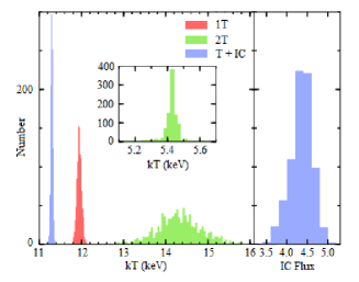
Figure 11: The distribution of best-fit parameter values for the 1T (red), 2T (green), and T$+$IC (blue) models using the 1000 realizations of the background (as described in Section 3.3). Parameters shown are the temperatures of each model and the IC flux (from 20–80 keV) in units of $10^{-12}$ erg s^-1 cm^-2. The width of the distributions shows the effects that systematic uncertainties in our modelling have on these parameters, which are also reported in Table 2.

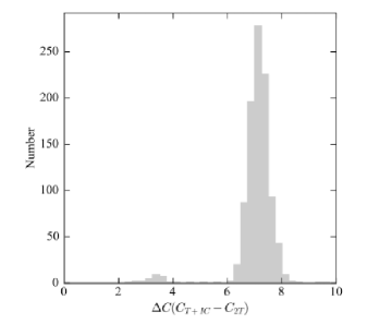
Figure 12: The distribution of the difference in C-stat values ($\Delta$$C$) between the T$+$IC and 2T models from fits using the 1000 realizations of the background. The 2T model is statistically better ($\sim$2.5$\sigma$ on average) at describing the NuSTAR-observed spectra than the T$+$IC model, with no realizations favoring it over the 2T model. Therefore, we conclude that the data clearly disfavor the addition of a non-thermal component.

5 Summary and Discussion

NuSTAR observed A2163 for a time period of 115 ks which was then cleaned down to 112 ks after a manual filtering process. Prior to searching for a non-thermal signal, a detailed background emission model was applied to subtract background data from our spectra.

5.1 Non-thermal Emission

Based on our T$+$IC model, we can set a 90% upper limit on the 20–80 keV flux of non-thermal emission coming from A2163 of $F_{\rm NT}$ $<$ 4.03 $\times$ $10^{-12}$ erg s^-1 cm^-2 using the T$+$IC model or $F_{\rm NT}$ $<$ 1.64 $\times$ $10^{-12}$ erg s^-1 cm^-2 using the 9T$+$IC model. As discussed in Section 4.2.5, we can confidently rule out IC scattering when comparing the fits including a power law model to fits including two temperature models. The data favors a purely thermal model with two different components describing the variations in temperature across the cluster. It is important to note that the histogram in Figure 11 still shows IC fluxes despite our claims that there is no significant detection. This presence is due to the IC flux masquerading as an extra temperature component. Our 9T+IC upper flux limit, when including systematic errors, goes nearly to 0, further suggesting that the IC interpretation is rejected. The addition of an IC component does not describe the hard X-ray emission as well as the 2T model, at a confidence level of $\sim$2.5$\sigma$ based on Figure 12. Our non-thermal upper limit is an order of magnitude smaller than the limit obtained by Ota et al. (2014), $F_{\rm NT}<1.2\times 10^{-11}$ erg s^-1 cm^-2. Their constraint was limited by the sensitivity of the Suzaku HXD-PIN instrument. In comparison with the claimed detection from RXTE, $F_{\rm NT}\sim 1.1^{+1.7}_{-0.7}\times 10^{-11}$ erg s^-1 cm^-2, our limit is also an order of magnitude smaller. The sensitivity of both instruments were limited by their substantially larger, non-imaging FOVs that admitted more cosmic background; the collimator designs admitted emission from $\sim$1° solid angles. Their non-imaging nature means that the spatial origin of the detected emission is unknown; the hardest emission could be coming from bright point sources unassociated with the ICM, for instance.

NuSTAR’s focusing optics allows point and other sources to be identified and excluded or avoided and provides less source-contaminated background measurements to be made concurrently during the observation, while Suzaku and RXTE did not. On the other hand, the Beppo-SAX PDS, another non-imaging hard X-ray instrument, was able to monitor background conditions during observations by nodding between source and background fields. The instrument was still susceptible to nearby non-ICM sources, however. If the cosmic background is not properly subtracted, hard emission from AGN could masquerade as a non-thermal signal. Our limit is more consistent with that from the Beppo-SAX PDS ($F_{\rm NT}<5.6\times 10^{-12}$ erg s^-1 cm^-2) (Feretti et al., 2001).

5.2 Cluster Magnetic Field

With an upper limit on the IC flux, we can set a lower limit on the average magnetic field strength $B$ using the ratio of the radio flux ($F_{R}$) to the X-ray flux ($F_{X}$) and the ratio of frequencies in the radio and X-ray bands where those fluxes are measured, $\nu_{R}$ and $\nu_{X}$, respectively. A total diffuse radio flux of 90 mJy inside our global extraction region was determined from VLA observations at 1.4 GHz. The magnetic field for a power law energy distribution of electrons emitting both synchrotron and IC emission can be determined from:

$$B=C(p)(1+z)^{(p+5)/(p+1)}\times\\ \bigg{(}\frac{F_{R}}{F_{X}}\bigg{)}^{2/(p+1)}\bigg{(}\frac{\nu_{R}}{\nu_{X}}\bigg{)}^{(p-1)/(p+1)}\,,$$ (1)

where $p$ is the index of electron distribution ($N(E)\propto E^{-p}$ and related to the spectral index $\alpha$ by $p=2\alpha+1)$ and $C(p)$ is a proportionality constant (Rybicki & Lightman, 1979; Longair, 1994). This equation is just the extension of the relationship for one electron to a distribution of electrons at different energies and momenta. The ratio $F_{R}/F_{X}$ for a single electron is simply the ratio of the energy densities $U$ of the fields the electron is scattering:

$$\frac{F_{R}}{F_{X}}=\frac{U_{B}}{U_{\rm CMB}}=\frac{B^{2}/8\pi}{aT^{4}_{\rm CMB}}\,.$$ (2)

With the T$+$IC model we obtain a lower limit of $B>0.22~{}\mu$G, and with the 9T$+$IC model the limit is raised to 0.35 $\mu$G. These are both larger than previous limits quoted in Ota et al. (2014), which is B $>$ 0.098 $\mu$G for $\Gamma$ = 2.18 and $B>0.006~{}\mu$G when using $\Gamma=1.5$. The radio flux used in their work was 155 mJy at the same 1.4 GHz frequency. This varies from ours due to our smaller extraction region, which excluded roughly half the flux used in their study. Our limits both fall short of the $B=0.4\pm 0.2~{}\mu$G estimate found by Rephaeli et al. (2006). This limit is higher than ours due to different assumptions made about the distribution of relativistic electrons (as shown by the use of the spectral energy index $\Gamma=1.6$ in their study). When using this value in our equation, our magnetic field limits increase by roughly 0.3 $\mu$G, consistent with the conflict in IC fluxes. Our lower limit is still short of the estimate for $B$ assuming equipartition conditions ($B=0.64~{}\mu$G; Feretti et al., 2004). These conditions assume that the total energy of a synchrotron source is distributed between fields and particles. An estimate for the total energy is taken at the minimum value. This condition is obtained by setting the magnetic field energy contributions equal to the contributions from the relativistic particles. Just like our non-thermal flux limit, our magnetic field most closely agrees with the lower limited estimated from Beppo-SAX of 0.28 $\mu$G (Feretti et al., 2001).

5.3 Temperature Map

While the focus of this paper is on the non-thermal emission present in the cluster, we also briefly analyzed various regions of interest throughout the cluster loosely based on the work done by Bourdin et al. (2011). These regions and their temperatures are shown in Figure 6 and Table 1. Compared to the previously referenced temperature map, created from XMM-Newton data, we noticed the absence of high temperature ($\sim$18 keV) gas in the northeast of the cluster (region 9). A2163 lies somewhat near the Galactic plane in a region of high neutral hydrogen column density. If its distribution varies on small angular scales toward the cluster, but it is modeled as constant across the FOV, temperature estimates will be skewed by the fitting procedure, which is weighted to focus the fit quality on the lower energy portion of spectra, where the count rate is higher. If this variation is taken into account, as was done in Bourdin et al. (2011), then another potential issue is model bias. In a future work (described in slightly more detail in the following section) we will be showing that depending on model selection (i.e. including molecular absorption and using different $n_{H}$ fitting models) the 18 keV gas can disappear entirely in the XMM-Newton. NuSTAR’s insensitivity to foreground absorption at the level present in A2163 removes this potential bias.

5.4 Future Work

In future work, we will revisit the topic of non-thermal emission locally within the cluster using XMM-Newton and Chandra data to provide broad band, spatially resolved joint spectral fits with the NuSTAR data. If diffuse, non-thermal emission is more localized in the ICM, this approach could prove sensitive enough to detect it. However, due to uncertainties in the absorption and cross-correlation factors, we don’t expect much improvement to the global constraint on IC emission from A2163. We will also revisit the temperature map presented in Figure 6 and test the variable absorption hypothesis discussed in Section 4.2.4 with joint fits of NuSTAR spectra with the aforementioned spatially coincident spectra from archival XMM-Newton and Chandra observations.

Appendix A ARF Generation

A.1 Issue with numkarf-generated ARFs

During the analysis, we encountered a problem with the ARF generation routine numkarf included in nuproducts. The error is likely due to how the ARF is normalized using an unvignetted exposure map. The issue arises when the extended=yes flag is set, and it appears to be caused by something specific in this particular observation. When the problem was initially discovered, a bug was found and fixed within nuexpomap, which caused the optical axis to be offset from its true location. Unfortunately, that bug appears unrelated to this issue, or more precisely, its fix did not fully solve the issue with ARF generation.

To illustrate the issue, ARFs were created for several small circular regions, shown in Figure 13. Small region sizes were chosen so that the ARFs would be similar for a region regardless of how they were created. Both point source extended=no and extended extended=yes ARFs were generated, with the latter set more appropriate for diffuse ICM emission. The region labeled “Ref” is nearest the average position of the optical axis; we plot all ARFs relative to this ARF in Figure 14. The point source ARFs (left panel) show the expected behavior, with farther off-axis region ARFs having both lower overall normalization and proportionately lower areas at higher energies, consistent with the vignetting properties of NuSTAR. While the extended ARFs (middle panel of Fig. 14) exhibit similar energy dependence as their corresponding point source ARFs, their overall normalizations do not.

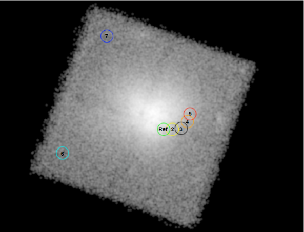
Figure 13: The extraction regions used to check extended ARF generation with nuproducts; their labels and colors correspond those used in Figure 14. The reference region is placed near the location of the optical axis, which was determined using a vignetted exposure map at 10 keV.

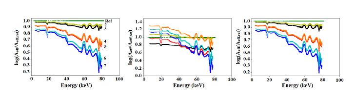
Figure 14: Left: Point source ARFs, scaled by the Ref ARF (green line) representing the normalized ARF obtained from a region located near the optical axis. As expected, ARFs extracted from surrounding regions fall below the line, with effective area dropping more dramatically both in energy and in distance from the optical axis. Middle: ARFs generated using nuproducts to generate extended ARFs from the same regions. While the energy dependence of the ARF appears to be properly captured in each case, the overall normalizations are clearly incorrect. Right: ARFs generated using a custom script meant to apply the correct overall normalization to extended ARFs. All plots shown are from Telescope A. The same trend is seen in Telescope B.

A.2 Custom ARF generation

Point source ARFs are generated following the methodology employed by numkarf, albeit with independent code; test ARFs made across the FOV differ by $<$1% at all energies from those made with numkarf. Extended ARFs are similarly produced as well in theory, although the code was written without reference to the corresponding code in numkarf to avoid recreating the issue. First, point source ARFs are generated on a grid over the region with spacings set by a boxsize parameter (default set to 10 pixels). A weighted sum of these ARFs results in the final extended ARF. The weighting normalizes each ARF to either the fraction of the region area it covers (corresponding to a flat distribution of source emission) or the fraction of counts within the region, provided by a source image (generally taken to be a background-subtracted NuSTAR ($E<20$ keV) or other X-ray image. In this implementation, chip gaps and excluded pixels are not corrected for, but the impact of these corrections should be minimal. It should be noted that for this process, we used the non-exposure corrected image at first. Upon testing, however, the exposure corrected image and our original attempt agree to within 0.8$\%$ of each other.

The right panel of Figure 14 shows the extended ARFs made with this method. While not identical to the numkarf-generated point source ARFs (as they shouldn’t be, even for such small regions), the ARFs are quite similar in both energy dependence and overall normalization, demonstrating that they have been accurately derived.

References

- Abell (1958) Abell, G. O. 1958, ApJS, 3, 211
- Arnaud (1992) Arnaud, M. 1992, A2163: an exceptionally hot cluster of galaxies., Tech. rep.
- Bahcall & Cen (1993) Bahcall, N. A., & Cen, R. 1993, ApJ, 407, L49
- Boldt (1987) Boldt, E. A. 1987, in NASA Conference Publication, Vol. 2464, 339–378
- Bourdin et al. (2011) Bourdin, H., Arnaud, M., Mazzotta, P., et al. 2011, A&A, 527, A21
- Carilli & Taylor (2002) Carilli, C. L., & Taylor, G. B. 2002, ARA&A, 40, 319
- Cassano et al. (2013) Cassano, R., Ettori, S., Brunetti, G., et al. 2013, ApJ, 777, 141
- Ettori et al. (2019) Ettori, S., Ghirardini, V., Eckert, D., et al. 2019, A&A, 621, A39
- Feretti et al. (2001) Feretti, L., Fusco-Femiano, R., Giovannini, G., & Govoni, F. 2001, A&A, 373, 106
- Feretti et al. (2004) Feretti, L., Orrù, E., Brunetti, G., et al. 2004, A&A, 423, 111
- Giovannini et al. (1999) Giovannini, G., Tordi, M., & Feretti, L. 1999, New A, 4, 141
- Govoni et al. (2004) Govoni, F., Markevitch, M., Vikhlinin, A., et al. 2004, ApJ, 605, 695
- Hansen et al. (2002) Hansen, S. H., Pastor, S., & Semikoz, D. V. 2002, ApJ, 573, L69
- Harrison et al. (2013) Harrison, F. A., Craig, W. W., Christensen, F. E., et al. 2013, ApJ, 770, 103
- Kalberla et al. (2005) Kalberla, P. M. W., Burton, W. B., Hartmann, D., et al. 2005, A&A, 440, 775
- Longair (1994) Longair, M. S. 1994, High energy astrophysics. Vol.2: Stars, the galaxy and the interstellar medium
- Markevitch et al. (1996) Markevitch, M., Mushotzky, R., Inoue, H., et al. 1996, ApJ, 456, 437
- Markevitch et al. (1994) Markevitch, M., Yamashita, K., Furuzawa, A., & Tawara, Y. 1994, ApJ, 436, L71
- Maurogordato et al. (2008) Maurogordato, S., Cappi, A., Ferrari, C., et al. 2008, A&A, 481, 593
- Million & Allen (2009) Million, E. T., & Allen, S. W. 2009, MNRAS, 399, 1307
- Ota et al. (2014) Ota, N., Nagayoshi, K., Pratt, G. W., et al. 2014, A&A, 562, A60
- Perley & Butler (2013) Perley, R. A., & Butler, B. J. 2013, ApJS, 204, 19
- Rephaeli (1979) Rephaeli, Y. 1979, ApJ, 227, 364
- Rephaeli et al. (2006) Rephaeli, Y., Gruber, D., & Arieli, Y. 2006, ApJ, 649, 673
- Rossetti et al. (2016) Rossetti, M., Gastaldello, F., Ferioli, G., et al. 2016, MNRAS, 457, 4515
- Rybicki & Lightman (1979) Rybicki, G. B., & Lightman, A. P. 1979, Radiative processes in astrophysics
- Vacca et al. (2018) Vacca, V., Murgia, M., Govoni, F., et al. 2018, Galaxies, 6, 142
- Vikhlinin et al. (2009) Vikhlinin, A., Murray, S., Gilli, R., et al. 2009, in astro2010: The Astronomy and Astrophysics Decadal Survey, Vol. 2010, 305
- Wik et al. (2014) Wik, D. R., Hornstrup, A., Molendi, S., et al. 2014, ApJ, 792, 48
- Willingale et al. (2013) Willingale, R., Starling, R. L. C., Beardmore, A. P., Tanvir, N. R., & O’Brien, P. T. 2013, MNRAS, 431, 394