Anomalous Floquet tunneling in uniaxially strained graphene

Abstract

The interplay of strain engineering and photon-assisted tunneling of electrons in graphene is considered for giving rise to atypical transport phenomena. The combination of uniaxial strain and a time-periodic potential barrier helps to control the particle transmission for a wide range of tunable parameters. With the use of the tight-biding approach, the elasticity theory, and the Floquet scattering, we found an angular shift of the maximum transmission in the sidebands for uniaxial strains breaking the mirror symmetry with respect to the normal incidence, which is called anomalous Floquet tunneling. We show that electron tunneling depends strongly on the barrier width, incident angle, uniaxial strain, and the tuning of the time-periodic potential parameters. An adequate modulation of the barrier width and oscillation amplitude serves to select the transmission in the sidebands. These findings can be useful for controlling the electron current through the photon-assisted tunneling being used in multiple nanotechnological applications.

I Introduction

Photon-assisted tunneling is a powerful tool for controlling electron current in a device through the illumination of a particular area of the system Dayem and Martin (1962); Hartman (1962); Tien and Gordon (1963); Shirley (1965); Büttiker and Landauer (1982); Fletcher (1985); Grossmann et al. (1991); Wagner (1994); Kouwenhoven et al. (1994); Wagner (1995); Blick et al. (1995); Wagner (1996); Wagner and Zwerger (1997); Platero and Aguado (2004); Zhang et al. (2006); Trauzettel et al. (2007); Schwede et al. (2010); Mueller et al. (2010); Freitag et al. (2012); Tielrooij et al. (2013); Ma et al. (2018); Gudmundsson et al. (2012); Biswas and Sinha (2013); Soltani et al. (2020). The tuning of the laser frequency and the intensity can serve to explore different features in quantum transport. The understanding of the interaction of electrons under external electromagnetic fields has led to a huge number of technological applications. Nevertheless, there are many unusual electronic transport effects in the presence of time-periodic potentials that requires an exhaustive study and revision from the new perspective given by the rising of two-dimensional materials Neto et al. (2009); Vogt et al. (2012); Li et al. (2014); Wehling et al. (2014); Carvalho et al. (2016); Li et al. (2018); Betancur-Ocampo et al. (2019, 2020); Biswas et al. (2019). Most of these materials belong to the classification of Dirac matter, where the Dirac-Weyl equation describes the dynamics of low energy excitations Neto et al. (2009); Wehling et al. (2014); Díaz-Bautista and Betancur-Ocampo (2020); Setare et al. (2019); Díaz-Bautista et al. (2019); Dell’Anna et al. (2018); Majari et al. (2017); Yang et al. (2019); Ren et al. (2019); Ghosh and Roy (2019); Le et al. (2020). While that, the Floquet scattering formalism has been the most recurrent theory for depicting the dynamics of photon-assisted tunneling Li and Reichl (1999); Moskalets and Büttiker (2002); Gu et al. (2011); Bilitewski and Cooper (2015); Savel’ev and Alexandrov (2011). This approach allows a simplified vision of electron tunneling through sidebands. Electrons impinging the oscillating potential barrier are reflected or refracted from different energy channels by the absorption or emission of one or multiple photons Li and Reichl (1999); Wurl and Fehske (2019); Zeb et al. (2008); Cao et al. (2011); Sattari and Mirershadi (2020); Jongchotinon and Soodchomshom (2020); Yan (2017); Jellal et al. (2014); Savel’ev et al. (2012); Szabó et al. (2013); Chen (2015); Schulz et al. (2015). In this way, Floquet scattering has been used successfully for explaining the constructive interference of continuum and bound states in quantum wells, an effect known as Fano resonances Fano (1961); Göres et al. (2000); Kobayashi et al. (2002); Miroshnichenko et al. (2010); Lu et al. (2012); Myoung et al. (2013); Zhang et al. (2015). Other interesting phenomena have been predicted based on the Floquet scattering theory, among them the Wigner delay times Sattari and Mirershadi (2020), Hartman effect Kh and Faizabadi (2018), suppression of Klein tunneling Zeb et al. (2008); Biswas and Sinha (2013); Sinha and Biswas (2012); Yampol’skii et al. (2008), Floquet topological insulators Calvo et al. (2011); Usaj et al. (2014); Perez-Piskunow et al. (2015); Savel’ev and Alexandrov (2011); Cayssol et al. (2013); Wintersperger et al. (2020); Wang et al. (2013); Mahmood et al. (2016); Afzal et al. (2020), non-Hermitian Floquet invisibility Longhi (2017), and photo-electronic induced emission Liang et al. (2013); Sun et al. (2012); Tao et al. (2020).

The interplay between strain engineering and photon-assisted tunneling may open more possibilities, due to the increment of external variables to control the electron tunneling. By applying strain in graphene and related materials, the electronic band structure is modified drastically and serves to modulate the electronic, optical, and transport properties Pereira et al. (2009); Pereira and Neto (2009); Pereira et al. (2010); Ribeiro et al. (2009); Cocco et al. (2010); Pellegrino et al. (2010); Choi et al. (2010); Naumis et al. (2017); Naumov and Bratkovsky (2011); Rostami and Asgari (2012); Barraza-Lopez et al. (2013); Assili et al. (2015); Guinea et al. (2009); Levy et al. (2010); Haddad and Mandhour (2018); Sahalianov et al. (2018); Contreras-Astorga et al. (2020); Zahidi et al. (2020); Concha et al. (2018); Lee et al. (2015); Midtvedt et al. (2016); Pérez-Pedraza et al. (2020). Inhomogeneous strain gave rise to the emergence of valleytronics and pseudo-magnetic fields Guinea et al. (2009); Levy et al. (2010); Wu et al. (2011); Rechtsman et al. (2012); Stegmann and Szpak (2016, 2019). Outstanding electron optics-like effects appear in uniaxially strained graphene Betancur-Ocampo (2018); Díaz-Bautista and Betancur-Ocampo (2020). Such a system displayed partial positive refraction in asymmetric Veselago lenses, a negative reflection of electrons, and anomalous Klein tunneling Betancur-Ocampo (2018); Zhang and Yang (2019); Betancur-Ocampo et al. (2019). Those theoretical results may be tested not only in uniaxially strained graphene but also hexagonal optical lattices and photonic crystals Wintersperger et al. (2020); Tarruell et al. (2012); Rechtsman et al. (2012). Recently, a time periodic potential in optical lattices was experimentally realized in Wintersperger et al. (2020). Photonic crystal emulations of strained graphene evidenced that Klein tunneling persists for deformations along the zig-zag and armchair directions Bahat-Treidel et al. (2010).

In this paper, we show that the combination of photon-assisted tunneling and strain engineering present singular transmission effects. The application of uniaxial strain causes a strong anisotropy in the electron tunneling. Dependent on the amplitude of time-periodic potential and frequency, there are preferential incidence angles for electron tunneling in the sidebands. We find suppression of the anomalous Klein tunneling, which can be useful for electronic confinement. Moreover, the tuning of potential barrier width serves to select the transmission in sidebands in order to produce photo-induced electronic current.

The paper is structured as follows: In section II, we give a short review of how the tight-binding approach and elasticity theory is useful for the development of a strain-modified Hamiltonian in graphene and related anisotropic hexagonal lattices. In section III, we apply the Floquet scattering theory in order to analyze the transmission features of a fully strained graphene sheet with time-periodic potential barrier. We present in IV the results of our numerical and analytical calculations of the transmission probabilities for the sidebands. We expose the conclusions and final remarks in section V.

II Dirac-Weyl Hamiltonian of uniaxially strained graphene

(a)	(b)

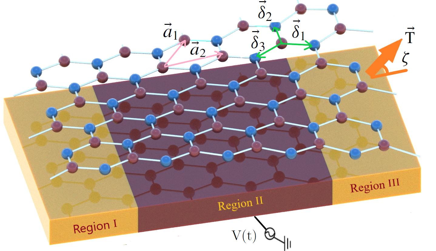
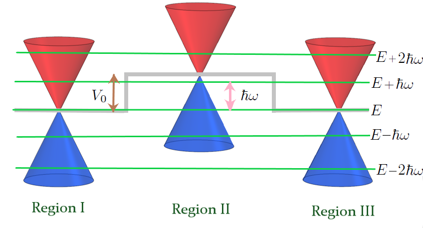
Figure 1: (a) Schematic representation of uniaxially strained graphene in a time-periodic potential. Violet and blue circles indicate the sites of triangular sublattices A and B, respectively. The vector $\boldsymbol{T}$ corresponds to the applied tension in the $\zeta$ direction. Each nearest-neighbor possesses a hopping parameter $\tau_{j}$ and bond length $\delta_{j}$. The quantities $\boldsymbol{a}_{1}$ and $\boldsymbol{a}_{2}$ are the deformed lattice vectors. The external gates induce a time-periodic potential barrier in region II. (b) Description of the Floquet scattering across the time-periodic potential and Dirac cone structure. Horizontal green lines represent the energy channels $E-m\hbar\omega$, where transmission in the sidebands occur.

Uniaxially strained graphene and anisotropic hexagonal lattices are composed by two deformed triangular sublattices $A$ and $B$ with a basis of two atoms per unit cell, as shown in Fig. 1(a). According to the elasticity theory, the application of a uniaxial strain deformes the lattice vectors in the pristine configuration, and they are given by Pereira et al. (2009); Betancur-Ocampo (2018); Díaz-Bautista and Betancur-Ocampo (2020)

$$\boldsymbol{a}_{1}=(a_{1x},a_{1y}) = \sqrt{3}a(1+\rho^{-}\epsilon+\rho^{+}\epsilon\cos 2\zeta,\rho^{+}\epsilon\sin 2\zeta)$$

$$\boldsymbol{a}_{2}=(a_{2x},a_{2y}) = \frac{\sqrt{3}}{2}a(1+\rho^{-}\epsilon+2\rho^{+}\epsilon\cos(2\zeta-60^{\circ}),$$

$$\sqrt{3}(1+\rho^{-}\epsilon)+2\rho^{+}\epsilon\sin(2\zeta-60^{\circ})),$$

where the constants $\rho^{\pm}$ are defined as

$$\rho^{\pm}=\frac{1}{2}(1\pm\nu)$$ (2)

and $\nu=0.18$ is the Poisson ratio, while $a=0.142$ nm is the bond length in pristine graphene Neto et al. (2009). The vectors $\boldsymbol{\delta}_{j}$ with $j=1,2$ and $3$ indicate the three nearest neighbors site on the underlying sublattice $A$, as shown in Fig. 1(a). The strain parameters $\epsilon$ and $\zeta$ quantify the percentage of tensile strain and the direction of the applied tension $\boldsymbol{T}$ with respect to the $x$ axis. The failure strain has been estimated to occur at the approximated value $\epsilon\approx 28\%$ Cadelano et al. (2009); Lee et al. (2008). However, we use a moderated range of $\epsilon$ from 0 to 10$\%$ in all our calculations within the linear elastic regimen, where Tight-Binding (TB) and Density Functional Theory (DFT) calculations have been demonstrated to have a good agreement Ribeiro et al. (2009). Nevertheless, controlled and reversible extreme strains $\epsilon>10\%$ has been realized experimentally Garza et al. (2014). Using the TB approach to first nearest neighbors, we consider one orbital per atom in the unit cell and neglect the overlap orbital among neighboring sites. The scaling rule $\tau_{j}=\tau\exp[-\beta(\delta_{j}/a-1)]$ relates the hopping parameters $\tau_{j}$ with the deformed bond lengths $\delta_{j}$. In graphene, $\beta=2.6$ is the Grüneisen constant and $\tau=2.7$ eV is the isotropic hopping Wong et al. (2012); Neto et al. (2009). This scaling rule evidences that the Fermi velocity is anisotropic and has a tensorial character. In the Fourier basis and expanding around the Dirac cone, the Hamiltonian is Betancur-Ocampo (2018); Díaz-Bautista and Betancur-Ocampo (2020)

$${{H}_{D}}=\hbar\begin{bmatrix}0&\boldsymbol{v}^{c*}\cdot\boldsymbol{k}\\ \boldsymbol{v}^{c}\cdot\boldsymbol{k}&0\end{bmatrix},$$ (3)

where $\boldsymbol{k}=(k_{x},k_{y})$ is the wave vector and

$$\boldsymbol{v}^{c}=(v^{c}_{x},v^{c}_{y})=\frac{i}{\hbar}\left(\boldsymbol{a}_{1}\tau_{1}{e}^{-i\boldsymbol{K}_{D}\cdot\boldsymbol{\delta}_{1}}+\boldsymbol{a}_{2}\tau_{2}{e}^{-i\boldsymbol{K}_{D}\cdot\boldsymbol{\delta}_{2}}\right),$$ (4)

are the complex velocities, being $\boldsymbol{K}_{D}$ the Dirac point position, which is the solution of

$$\sum^{3}_{j=1}\tau_{j}{e}^{-i\boldsymbol{K}_{D}\cdot\boldsymbol{\delta}_{j}}=0.$$ (5)

The Hamiltonian (3) is the Dirac-Weyl type $H=v_{ij}\sigma_{i}p_{j}$, where $v_{ij}$ is the Fermi velocity tensor and $p_{j}=\hbar k_{j}$ are the components of linear momentum. The electronic band structure of anisotropic hexagonal lattice, in the semimetallic phase, present generally elliptical and rotated Dirac cones. The dispersion relation

$$E=s\hbar|\boldsymbol{v}^{c}\cdot\boldsymbol{k}|$$ (6)

of the Hamiltonian (3) displays this cone around the Dirac point in the reciprocal space, where $s$ is the band index Betancur-Ocampo (2018). The eigenstates of the Dirac-Weyl-like Hamiltonian (3) have the form

$$\boldsymbol{\Phi}_{s,\boldsymbol{k}}(\boldsymbol{r})=\frac{1}{\sqrt{2}}\binom{1}{se^{i\phi(\boldsymbol{k})}}e^{i\boldsymbol{k}\cdot\boldsymbol{r}}$$ (7)

and the definition of pseudospin angle $\phi(\boldsymbol{k})$ is

$$\tan\phi(\boldsymbol{k}) = \frac{-v_{x}k_{x}\sin\mu_{x}+v_{y}k_{y}\sin\mu_{y}}{v_{x}k_{x}\cos\mu_{x}+v_{y}k_{y}\cos\mu_{y}},$$ (8a)

$$v^{c}_{x} = v_{x}e^{-i\mu_{x}},$$ (8b)

$$v^{c}_{y} = v_{y}e^{i\mu_{y}}.$$ (8c)

Here $v_{x,y}^{c}$ are the $x$- and $y$-components of the complex vector $\boldsymbol{v}^{c}$ with norm $v_{x,y}$ and phase $\mu_{x,y}$. The pseudo-spin direction, wave vector, and the group velocity are generally not parallel.

The direction of group velocity is found to be Betancur-Ocampo (2018)

$$\tan\theta=\frac{v^{2}_{y}k_{y}+v_{x}v_{y}k_{x}\cos(\mu_{x}+\mu_{y})}{v^{2}_{x}k_{x}+v_{x}v_{y}k_{y}\cos(\mu_{x}+\mu_{y})}$$ (9)

and allows to obtain the wave vector in terms of incidence angle. The application of uniaxial strains out of the zig-zag and armchair direction have led to the emergence of anomalous Klein tunneling Betancur-Ocampo (2018), which occurs at the incidence angle

$$\theta_{KT}=\arctan[v_{y}\cos(\mu_{x}+\mu_{y})/v_{x}]$$ (10)

when $k_{y}=0$ in Eq. (9).

We now rewrite the dispersion relation (6) in the more explicit form

$$E =s\hbar\sqrt{k_{x}^{2}v_{x}^{2}+2k_{y}k_{x}v_{x}^{2}\tan\theta_{KT}+k_{y}^{2}v_{y}^{2}}.$$ (11)

In next sections, we shall evidence that this symmetry breaking with respect to the $x$ axis modifies drastically the electron transmission for the sidebands.

III Photon-assisted tunneling through a time-periodic potential barrier

We study the tunneling of electrons in uniaxially strained graphene under the presence of a time-periodic potential barrier, as shown in Fig. 1. The photon-assisted mechanism, such as a time-periodic potential used here, causes the appearance of many sidebands Li and Reichl (1999); Zeb et al. (2008); Sinha and Biswas (2012). These sidebands correspond to multiple copies of the dispersion relation with a relative energy separation $\hbar\omega$, where $\hbar$ and $\omega$ is the Planck constant and the potential frequency, respectively. The Floquet scattering is the usual theory to describe the tunneling of a single electron with energy $E$ to cross the time-periodic potential gaining or losing the energy quantity $m\hbar\omega$, where $m=0,\pm 1,\pm 2,\ldots$ indicates the sideband (see Fig. 1(b)). The tunneling is elastic (inelastic) if the electron crosses the oscillating barrier without (with) changes in the energy. Most of the experimental realizations that involved photon-assisted tunneling are observed generally in the frequency range from the microwave to infrared electromagnetic spectrum Dayem and Martin (1962); Blick et al. (1995); Kouwenhoven et al. (1994); Platero and Aguado (2004); Schwede et al. (2010); Mueller et al. (2010); Freitag et al. (2012); Tielrooij et al. (2013); Ma et al. (2018); Sun et al. (2012); Wang et al. (2013); Mahmood et al. (2016); Soltani et al. (2020); Tao et al. (2020).

We have several external variables to control the electron tunneling by means of the application of uniaxial strain and tuning of amplitude, frequency, barrier height and width of the time-periodic potential. From a general point to view, we write the time-dependent Schrödinger equation as

$$[H(\boldsymbol{p})+V(\boldsymbol{r},t)]\psi(\boldsymbol{r},t)=i\hbar\partial_{t}\psi(\boldsymbol{r},t),$$ (12)

where $H(\boldsymbol{p})$ can be a general Hamiltonian that depends only on the linear momentum $\boldsymbol{p}$. Therefore, the following development from Eqs. (12) to (18) can be applied to multiple systems in condensed matter to depict the Floquet scattering of electrons in the presence of a time-periodic potential barrier.

The eigenvectors of $H(\boldsymbol{p})$ are the wave functions $\boldsymbol{\Phi}_{s,\boldsymbol{k}}(\boldsymbol{r})$ of the electron belonging to the momentum $\boldsymbol{k}$ and band index $s$. For instance, in the particular Hamiltonian (3) the wave functions $\boldsymbol{\Phi}_{s,\boldsymbol{k}}(\boldsymbol{r})$ are given by (7). We define ${\cal E}(s,\boldsymbol{k})$ to be the corresponding eigenvalue

$$H(\boldsymbol{p})\boldsymbol{\Phi}_{s,\boldsymbol{k}}(\boldsymbol{r})={\cal E}(s,\boldsymbol{k})\boldsymbol{\Phi}_{s,\boldsymbol{k}}(\boldsymbol{r}).$$ (13)

The time-periodic potential is given by

$$V(x,t)=\begin{cases}V_{0}+V_{1}\cos(\omega t),\;\;\textrm{for}\;\;{0}<x<{D}\\ 0,\;\;\textrm{otherwise}\end{cases}$$ (14)

To solve this, we divide the system in three regions, namely $x\leq 0$, $0\leq x\leq D$ and $D\leq x$, denoted by I, II, and III respectively. We define

$$\alpha=\frac{V_{1}}{\hbar\omega}$$ (15)

and find the general plane wave solutions for all three regions:

$$W_{s_{\text{I}}\boldsymbol{k}_{\text{I}}}(\boldsymbol{r},t) = \boldsymbol{\Phi}_{s_{\text{I}},\boldsymbol{k}_{\text{I}}}(\boldsymbol{r})\exp\left[-i{\cal E}(s_{\text{I}},\boldsymbol{k}_{\text{I}})t/\hbar\right]$$ (16a)

$$W_{s_{\text{II}}\boldsymbol{k}_{\text{II}}}(\boldsymbol{r},t) = \boldsymbol{\Phi}_{s_{\text{II}},\boldsymbol{k}_{\text{II}}}(\boldsymbol{r})\exp\left[-(i/\hbar)\big{(}V_{0}t\right.$$ (16b)

$$\qquad\left.+{\cal E}(s_{\text{II}},\boldsymbol{k}_{\text{II}})t+V_{1}\sin(\omega t)/\omega\big{)}\right]$$

$$= \boldsymbol{\Phi}_{s_{\text{II}},\boldsymbol{k}_{\text{II}}}(\boldsymbol{r})\sum_{m=-\infty}^{\infty}J_{m}(\alpha)\exp\left[-(i/\hbar)\big{(}V_{0}\right.$$

$$\qquad\left.+{\cal E}(s_{\text{II}},\boldsymbol{k}_{\text{II}})+m\hbar\omega\big{)}t\right]$$

$$W_{s_{\text{III}}\boldsymbol{k}_{\text{III}}}(\boldsymbol{r},t) = \boldsymbol{\Phi}_{s_{\text{III}},\boldsymbol{k}_{\text{III}}}(\boldsymbol{r})\exp\left[-i{\cal E}(s_{\text{III}},\boldsymbol{k}_{\text{III}})t/\hbar\right]$$ (16c)

The second equality in (16b) follows from the identity

$$\exp\left[-i\alpha\sin(\omega t)\right] = \sum_{m=-\infty}^{\infty}J_{m}(\alpha)e^{-im\omega t},$$ (17)

where $J_{m}(\alpha)$ are Bessel functions of the first kind. We now determine linear superpositions of these various solutions $\boldsymbol{\Phi}_{s_{\text{I}},\boldsymbol{k}_{\text{I}}}(\boldsymbol{r},t)$, $\boldsymbol{\Phi}_{s_{\text{II}},\boldsymbol{k}_{\text{II}}}(\boldsymbol{r},t)$, and $\boldsymbol{\Phi}_{s_{\text{III}},\boldsymbol{k}_{\text{III}}}(\boldsymbol{r},t)$ in such a way as to yield continuous behaviour at the interfaces $x=0$ and $x=D$ for all times.

We assume that the incoming wave in region I is characterized by a wave vector $\boldsymbol{k}_{0}$ and a band index $s_{0}$. To match this in region II, we need all momenta $\boldsymbol{q}_{m}$ such that

$$E := {\cal E}(s_{0},\boldsymbol{k}_{0})={\cal E}(s_{m}^{\prime},\boldsymbol{q}_{m}^{\pm})+V_{0}+m\hbar\omega$$ (18a)

$$k_{y,0} = q_{y,m}^{\pm},$$ (18b)

where the second relation follows from the conservation of $k_{y,0}$ at all interfaces. The expressions (18a) are the sidebands for the system described by the Hamiltonian $H(\boldsymbol{p})$ in the presence of the time-periodic potential $V(x,t)$. Using the specific Hamiltonian of uniaxially strained graphene (3) in this general development, we have

$$q_{m,x}^{\pm} = \pm s^{\prime}_{m}\sqrt{\frac{(E-V_{0}-m\hbar\omega)^{2}}{\hbar^{2}v_{x}^{2}}-{\frac{v^{2}_{y}}{v^{2}_{x}}k_{y,0}^{2}\sin^{2}(\mu_{x}+\mu_{y})}}$$ (19a)

$$-k_{y,0}\tan\theta_{KT},$$

$$s_{m}^{\prime} = \,\mbox{\rm sgn}(E-V_{0}-m\hbar\omega),$$ (19b)

where the $\pm$ sign indicates the two possible solutions for $q_{m}$, which are obtained by the dispersion relation (11). There are two states with these wave vectors $q_{m}$ and the same energy, we shall use them to represent “left-going” and “right-going” waves in region II, in the same way as it would happen with $k_{x}$ and $-k_{x}$ in isotropic systems.

(a)	(b)	(c)

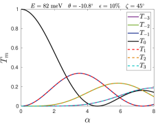
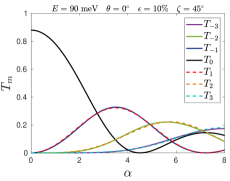
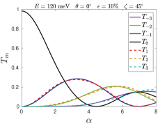
Figure 2: Transmission probability $T_{m}=|t_{m}|^{2}$ for electrons with energy $E$ from the central band to cross the oscillating barrier and lie on the sideband $E-m\hbar\omega$. This transmission is obtained from the numerical solution of the linear equation system (31b), as a function of the ratio $\alpha=V_{1}/\hbar\omega$, where $V_{1}$ is the oscillation amplitude for a time-periodic potential of height $V_{0}=200$ meV, width $D=100$ nm, and frequency $\omega=5$ THz. The set of uniaxial strain parameters are $\epsilon=10\%$ and $\zeta=45^{\circ}$. Transmission probability for the cases of anomalous Klein tunneling in the incidence angle $\theta_{KT}=-10.8^{\circ}$ and using the energy $E=82$ meV in (a), normal incidence in (b) and (c) for the energies $E=90$ and $120$ meV, respectively.

Now, in order to match the $e^{-im\omega t}$ behaviour in region II, we must introduce the wave vectors $\boldsymbol{k}_{m}$ in regions I and III, defined by

$${\cal E}(s_{m},\boldsymbol{k}_{m}^{\pm}) = E-m\hbar\omega$$ (20a)

$$k_{y,0} = k_{y,m}^{\pm}.$$ (20b)

Note again that $\boldsymbol{k}_{m}^{\pm}$ are uniquely determined by $\boldsymbol{k}_{0}$. Also, the $\pm$ sign is related to a choice of left-going and out-going waves, see (21a). Similarly, the solution of (20) is given by:

$$k_{x,m}^{\pm} = \pm s_{m}\sqrt{\frac{(E-m\hbar\omega)^{2}}{\hbar^{2}v_{x}^{2}}-{\frac{v^{2}_{y}}{v^{2}_{x}}k_{y,0}^{2}\sin^{2}(\mu_{x}+\mu_{y})}}$$ (21a)

$$-k_{y,0}\tan\theta_{KT},$$

$$s_{m} = \,\mbox{\rm sgn}(E-m\hbar\omega).$$ (21b)

It is possible to express $k_{y,0}$ in terms of the incidence angle $\theta$ inverting Eq. (9)

$$k_{y,0}=\frac{v_{x}|E|(\tan\theta-\tan\theta_{KT})}{\hbar v^{2}_{y}\sin^{2}(\mu_{x}+\mu_{y})\sqrt{1+\frac{v^{2}_{x}(\tan\theta-\tan\theta_{KT})^{2}}{v^{2}_{y}\sin^{2}(\mu_{x}+\mu_{y})}}}.$$ (22)

We now make the following Ansatz for the wave function $\boldsymbol{\psi}(\boldsymbol{r},t)$ in terms of the band index and wave vector values in the three different regions I, II, and III:

$$\boldsymbol{\psi}^{I}(\boldsymbol{r},t) = \frac{1}{\sqrt{2}}e^{ik_{y,0}y}e^{-iEt/\hbar}\left[\binom{1}{s_{0}e^{i\phi^{+}_{0}}}e^{ik^{+}_{x,0}x}\right.$$

$$+\left.\sum_{m=-\infty}^{\infty}r_{m}\binom{1}{s_{m}e^{i\phi^{-}_{m}}}e^{ik^{-}_{x,m}x}e^{-im\omega t}\right],$$

$$\boldsymbol{\psi}^{II}(\boldsymbol{r},t) = \frac{1}{\sqrt{2}}e^{ik_{y,0}y}e^{-iEt/\hbar}\!\!\!\!\!\!\sum_{n,{m}=-\infty}^{\infty}\!\!\!\!\!\!J_{n}(\alpha)\left[t^{\prime}_{m}\binom{1}{s^{\prime}_{m}e^{i\xi^{+}_{m}}}\right.$$

$$\!\!\!\!\!\!\times e^{iq^{+}_{x,m}x}+\left.r^{\prime}_{m}\binom{1}{s^{\prime}_{m}e^{i\xi^{-}_{m}}}e^{iq^{-}_{x,m}x}\right]e^{-i{(n+{m})\omega}t},$$

$$\boldsymbol{\psi}^{III}(\boldsymbol{r},t) = \frac{1}{\sqrt{2}}e^{ik_{y,0}y}e^{-iEt/\hbar}\!\!\!\!\sum_{m=-\infty}^{\infty}\!\!\!\!t_{m}\binom{1}{s_{m}e^{i\phi^{+}_{m}}}$$ (23c)

$$\qquad\qquad\times e^{ik^{+}_{x,m}x}e^{-im\omega t},$$

where we define the phases corresponding to the various wave vectors, as described in (8)

$$\phi_{m}^{\pm} = \phi(\boldsymbol{k}_{m}^{\pm})$$ (24)

$$\xi_{m}^{\pm} = \phi(\boldsymbol{q}_{m}^{\pm})$$ (25)

and we use the particular eigenstates (7). The coefficient $r_{m}$ is the reflection amplitude of the incident wave back into region I, $t^{\prime}_{m}$ and $r^{\prime}_{m}$ are the amplitudes of the right-going and left-going waves in region II respectively, and $t_{m}$ is the total transmission amplitude from I to III, while gaining or losing an energy $m\hbar\omega$ in the process. The sideband index indicates the conduction ($s^{\prime}_{m}=1$) or valence ($s^{\prime}_{m}=-1$) band.

With the matching of the wave functions (23) at $(x=0)$ and $(x=D)$ and using the orthonormality condition of Fourier basis, we obtain the following equations system

$$\delta_{m0}+r_{m} = \!\!\!\sum_{l=-\infty}^{\infty}J_{m-l}(\alpha)(t^{\prime}_{l}+r^{\prime}_{l})$$ (26a)

$$s_{m}\delta_{m0}e^{i{\phi}_{m}^{+}}+s_{m}r_{m}e^{i{\phi}_{m}^{-}} = \!\!\!\sum_{l=-\infty}^{\infty}s^{\prime}_{l}J_{m-l}(\alpha)\left(t^{\prime}_{l}e^{i{\xi}_{l}^{+}}\right.$$ (26b)

$$\quad+\left.r^{\prime}_{l}e^{i{\xi}_{l}^{-}}\right)$$

$$t_{m}e^{ik_{x,m}^{+}D} = \!\!\!\sum_{l=-\infty}^{\infty}J_{m-l}({\alpha})\left(t^{\prime}_{l}e^{iq_{x,l}^{+}D}\right.$$ (26c)

$$\left.\quad+r^{\prime}_{l}e^{iq_{x,l}^{-}D}\right)$$

$$s_{m}t_{m}e^{ik_{x,m}^{+}D}e^{i\phi_{m}^{+}} = \!\!\!\sum_{l=-\infty}^{\infty}s^{\prime}_{l}J_{m-l}({\alpha})\left(t^{\prime}_{l}e^{iq_{x,l}^{+}D}e^{i\xi_{l}^{+}}\right.$$ (26d)

$$\left.\qquad+r^{\prime}_{l}e^{iq_{x,l}^{-}D}e^{i\xi_{l}^{-}}\right)$$

The linear equations system (26) must be truncated up to a maximum number of terms because in principle, it is infinite. We can define this maximum number $L$ in the sum and impose the conditions

$$r_{m}=t^{\prime}_{m}=r^{\prime}_{m}=t_{m}=0\qquad(|m|\geq L+1).$$ (27)

In this way, the dimension of the system is $d\times d$, where $d=4(2L+1)$, and the sum index $m$ runs over $-L$ to $L$ in resemblance to the $L_{z}$ angular momentum quantization. We chose the ordered basis for the amplitude coefficients defining the vector of $d$ components by

$$\boldsymbol{X} = (r_{-L},\ldots,r_{L},t^{\prime}_{-L},\ldots,t^{\prime}_{L},r^{\prime}_{-L},\ldots,r^{\prime}_{L},t_{-L},\ldots,t_{L})^{\textrm{T}}$$ (28)

$$= \left[\big{(}r_{m}\big{)}_{m=-L}^{L}\big{(}t^{\prime}_{m}\big{)}_{m=-L}^{L}\big{(}r^{\prime}_{m}\big{)}_{m=-L}^{L}\big{(}t_{m}\big{)}_{m=-L}^{L}\right]^{\textrm{T}}$$

We now write the equations system (26) in a slightly more compact form as follows:

$${\mathcal{M}}_{1} = [-\mathcal{I}\mathcal{J}\mathcal{J}\mathcal{O}],$$ (29a)

$${\mathcal{M}}_{2} = [\mathcal{O}\mathcal{J}\mathcal{J}-\mathcal{I}],$$ (29b)

$$\mathcal{J} = {\mathcal{J}}_{ml}=J_{m-l}(\alpha),$$ (29c)

$${\mathcal{D}}_{1} = \,\mbox{\rm diag}\left[\left(s_{m}e^{i\phi_{m}^{-}}\right)_{m=-L}^{L}\left(s^{\prime}_{m}e^{i\xi_{m}^{+}}\right)_{m=-L}^{L}\right.$$ (29d)

$$\quad\ \left.\left(s^{\prime}_{m}e^{i\xi_{m}^{-}}\right)_{m=-L}^{L}\left(s_{m}e^{i\phi_{m}^{+}}\right)_{m=-L}^{L}\right],$$

$$\mathcal{D}_{2} = \,\mbox{\rm diag}\left[\left(e^{ik_{x,m}^{-}D}\right)_{m=-L}^{L}\left(e^{iq_{x,m}^{+}D}\right)_{m=-L}^{L}\right.$$ (29e)

$$\qquad\left.\left(e^{iq_{x,m}^{-}D}\right)_{m=-L}^{L}\left(e^{ik_{x,m}^{+}D}\right)_{m=-L}^{L}\right],$$

$$\boldsymbol{b}_{1} = \big{(}\delta_{m,0}\big{)}_{m=-L}^{L}\ ,$$ (29f)

$$\boldsymbol{b}_{2} = s_{0}e^{i\phi_{0}}\boldsymbol{b}_{1}$$ (29g)

where the square sub-matrices $\mathcal{I}$ and $\mathcal{O}$ are the identity and null matrix of size $d/4\times d/4$, respectively. Therefore, equations (26) can be written as ,

$$\mathcal{M}_{1}\boldsymbol{X} = \boldsymbol{b}_{1}$$ (30a)

$$\mathcal{M}_{1}\mathcal{D}_{1}\boldsymbol{X} = \boldsymbol{b}_{2}$$ (30b)

$$\mathcal{M}_{2}\mathcal{D}_{2}\boldsymbol{X} = \boldsymbol{0}$$ (30c)

$$\mathcal{M}_{2}\mathcal{D}_{1}\mathcal{D}_{2}\boldsymbol{X} = \boldsymbol{0}$$ (30d)

(a)	(b)	(c)

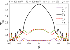
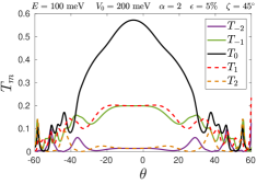
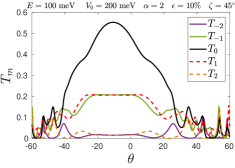
Figure 3: Anomalous Floquet tunneling of electrons at the energy $E=100$ meV as a function of the incidence angle $\theta$. The set of values for the time-periodic potential are $V_{0}=200$ meV, $D=100$ nm, and $\omega=5$ THz. Transmission probabilities $T_{m}=|t_{m}|^{2}$ using the strain parameters $\epsilon=0,5,10\%$ and $\zeta=45^{\circ}$ with $\alpha=2$ in (a), (b), and (c) respectively.

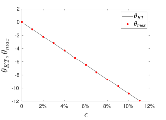
Figure 4: Anomalous Klein tunneling angle (Eq. (10)) and the numerically determined angular shift of the maximum transmission $T_{0}$ as a function of the tensile strain parameter $\epsilon$ at the direction $\zeta=45^{\circ}$ and the ratio $\alpha=V_{1}/\hbar\omega=2$.

On the one hand, we can identify that the rectangular matrices $\mathcal{M}_{1}$ and $\mathcal{M}_{2}$ control the scattering of electrons in the time-periodic potential barrier through a unique tunable parameter $\alpha$. On the other hand, the diagonal matrices $\mathcal{D}_{1}$ and $\mathcal{D}_{2}$ contain the effect of strain from the phases in (24) and wave vectors given by Eqs. (19a) and (21a). The photon-assisted tunneling amplitudes $t_{m}$ are provided by the last $2L+1$ components of vector

$$\boldsymbol{X} = \mathcal{M}^{-1}\boldsymbol{b},$$ (31a)

$$\mathcal{M} = [\mathcal{M}_{1}\quad\mathcal{M}_{1}\mathcal{D}_{1}\quad\mathcal{M}_{2}\mathcal{D}_{2}\quad\mathcal{M}_{2}\mathcal{D}_{1}\mathcal{D}_{2}]^{\textrm{T}}.$$ (31b)

Here $\cal{M}$ is the total square matrix of the system defined by Eqs. (26b)-(26d) and $\boldsymbol{b}=(\boldsymbol{b}_{1},\boldsymbol{b}_{2},\boldsymbol{0},\boldsymbol{0})$. Therefore, the coefficients are given by $T_{m}=|t_{m}|^{2}$ which quantify the transmission probabilities of electrons from the central band $E$ to cross the time-periodic potential barrier and transit to the sideband $E-m\hbar\omega$.

In appendix A, we show an approximate solution of this equation system with validity in the range $0<\alpha<1$.

IV Discussion and results

The application of uniaxial strain along the $\zeta=45^{\circ}$ changes drastically the transport properties in anisotropic hexagonal materials. Electrons impinging the electrostatic potential barrier at the specific incidence angle $\theta_{KT}$ present the anomalous Klein tunneling Betancur-Ocampo (2018). This effect emerges for strains that break the mirror symmetry with respect to the $x$ axis. We set the values $\epsilon=10\%$ and $\zeta=45^{\circ}$, where anomalous Klein tunneling appears for the incidence angle $\theta_{KT}=-10.8^{\circ}$ in the static barrier $\alpha=0$, (see Fig. 2(a)). This perfect transmission occurs when the wave vector is perpendicular to the barrier, as obtained setting $k_{y,0}=0$ in Eq. (9). The incidence angle is different to zero due to that the wave vector, pseudo-spin, and group velocities are generally not parallel Betancur-Ocampo (2018); Betancur-Ocampo et al. (2019). If we turn on the time-periodic potential, the anomalous Klein tunneling suppresses. The transmission probabilities in the central and sidebands depend on $\alpha$. In most of the cases, we only consider the transmission coefficients $T_{m}$ with $m=-2,-1,0,1,2$ because the other ones with $|m|>2$ have a maximum value smaller than 0.1 in the whole range of $0<\alpha<8$ and therefore, they can be neglected. The transmission probability $T_{m}$ starts to be relevant for $\alpha>|m|$, as shown in Fig. 2. We can see that electrons absorbing or emitting $m$ photons have the same probability to cross the barrier (see Fig. 2(a)). This equiprobability appears for the specific case where the wave vector is perpendicular to the barrier and also by the linear dispersion relation of electrons.

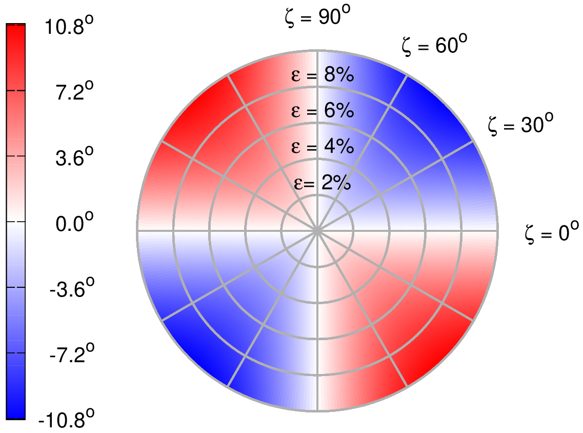
Figure 5: Anomalous Klein tunneling angle as a function of the strain parameters $\epsilon$ (radius from 0 to $10\%$) and $\zeta$ (polar angle in degrees).

(a)	(b)	(c)

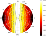
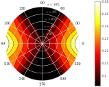
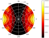
Figure 6: Transmission probability (a) $T_{0}$, (b) $T_{-1}$, and (c) $T_{-2}$ as a function of uniaxial strain parameters $\epsilon$ (radius from 0 to $10\%$) and $\zeta$ (polar angle in degrees) for electrons with normal incidence and energy $E=100$ meV in a time-periodic potential $V_{0}=200$ meV, $D=100$ nm, $\alpha=2$, and $\omega=5$ THz.

When electrons impinge under normal incidence to the time-periodic potential, as shown in Figs. 2(b) and (c), the wave vector is not perpendicular anymore as a consequence of the uniaxial strain out of the main axes $x$ and $y$. Hence, Klein tunneling deviates from the normal direction, and the transmission probability splits out slightly for the absorption and emission of photons, namely, $T_{m}\neq T_{-m}$. The perfect transmission for normal incidence by the Klein tunneling in the static case $\alpha=0$ is destroyed, as verified by changing the energy values to $E=90$ and $120$ meV in Fig. 2(b) and (c). This resonant tunneling is atypical for normal incidence.

(a)	(b)	(c)

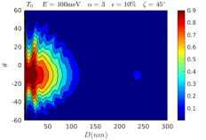
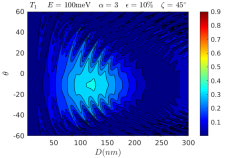
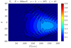
Figure 7: Transmission probabilities of (a) $T_{0}$, (b) $T_{1}$, and (c) $T_{2}$ as a function of barrier width and incidence angle for the potential height $V_{0}=200$ meV.

We call anomalous Floquet tunneling to the angular shift of the maximum transmission by the application of a uniaxial tension different to the direction $\zeta=0^{\circ}$ and $90^{\circ}$, as shown in Figs. 3 (a)-(c). Such a shift in the transmission probability usually appears in other systems by time-reversal symmetry breaking with an external magnetic field Sinha and Biswas (2012). That vector potential, which generates the magnetic field, shifts the Dirac cone in the reciprocal space. Although the strain here affects the Dirac cone differently, changing the circular shape to a rotated and elliptical one, both systems present a particular feature in common: incident electrons with a wave vector perpendicular to the interface have a nonzero parallel group velocity $v_{y}$. In Fig. 3, we chose a shortened incidence angle range to avoid the evanescent waves. The incident electrons have critical angles that depend on the sideband. Increasing $\epsilon$ in Figs. 3(a)-(c), we observe that this angular deviation in the maximum of transmissions improves. We show the angular shift of the maximum transmission $\theta_{max}$ as a function of the tensile strain in Fig. 4. This angular shift has a good agreement with the anomalous Klein tunneling angle $\theta_{KT}$ predicted by Eq. (10). It is worth noting that this angular shift of the maximum transmission depends only on the tensile strain $\epsilon$ and tension angle $\zeta$. The expansion of Eq. (10) (see appendix B), keeping only the first-order terms in $\epsilon$, we lead to a very simple and straightforward relation of the anomalous Klein tunneling angle with the parameters $\epsilon$ and $\zeta$

$$\theta_{KT}\approx\frac{360^{\circ}}{\pi}\rho^{+}(1-\beta)\epsilon\sin 2\zeta,$$ (32)

which has a negligible deviation of the exact relation (10) in the whole strain range considered. Uniaxial strain along with the directions $\zeta=0^{\circ}$ and $90^{\circ}$ (not shown) does not break the mirror symmetry with respect to the normal axis. In this case, the group velocity and the wave vector are parallel for normal incidence which restores the angular transmission symmetry. We quantify the anomaly in the transmissions using the direction of the Klein tunneling deviation in Eq. (10), which depends only on the strain parameters $\epsilon$ and $\zeta$. Fig. 5 shows this anomaly in the whole strain range. As expected, the uniaxial strains along the perpendicular and parallel directions to the interface keep the symmetry in the transmission. While tensions in a different direction to $\zeta\neq 0$ and $90^{\circ}$ cause the anomalous Floquet tunneling. We found that the highest angular shift value is $\theta_{KT}\approx-10.8^{\circ}$ for the set of parameters $\epsilon=10\%$ and $\zeta=45^{\circ}$.

(a)	(b)	(c)

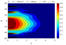
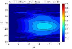
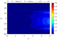
Figure 8: Transmission probabilities of (a) $T_{0}$, (b) $T_{1}$, and (c) $T_{2}$ as a function of the parameter $\alpha$ and incidence angle $\theta$ for the potential height $V_{0}=200$ meV and width $D=100$ nm.

To understand how the uniaxial strain affects the behavior of photon-assisted tunneling, we show the probability transmission as a function of $\epsilon$ and $\zeta$ in Fig. 6 for the case of normal incidence. We can see that in a wide range of $\zeta$, the behavior of $T_{m}$ is strongly anisotropic with the angle $\zeta$, and the increase of $\epsilon$ causes a reduction in the probability transmission $T_{0}$, as shown in Fig. 6(a). However, for the tension angle $\zeta=90^{\circ}$, normal incident electrons have an almost constant probability of crossing the barrier regardless of the tensile strain. It is worth noting that the independence of transmission on the tensile strain at $\zeta=90^{\circ}$ also appears for other sidebands, as shown in Fig. 6(b) and (c). The transmission $T_{1}$ and $T_{2}$ present an identical behavior with respect to the emission counterpart. The application of strain in the directions near the $x$-axis shows an increase of $T_{-1}$ and $T_{-2}$. While uniaxial strain along the $y$-axis decrease the electron transmission in the sidebands. The time exposition of electrons to the oscillating barrier explains the strain-induced transition from elastic to inelastic tunneling. Positive tensile strains in the direction $\zeta=0^{\circ}$ increase the bond lengths. Therefore, the probability amplitude of electrons decreases to hop among neighboring sites. In this way, there is more time exposition to interact with the time-periodic potential. Thus, electrons cross the barrier inelastically with transmission probabilities $T_{1}$ and $T_{2}$. In contrast, deformations parallel to the interface decrease the zigzag bond lengths, and electrons have a major probability to cross the barrier elastically.

We examine the behavior of the transmission probability $T_{m}$ as a function of barrier width and incidence angle, as shown in Fig. 7. In general, the reminiscence of the anomalous Klein tunneling makes that almost all the transmission occurs around the incident angle $\theta=-10.8^{\circ}$. We found that the tuning of barrier width can serve as a selector of the transmission in the sidebands. In thin barriers $D<50$ nm (see Fig. 7(a)), the transmission is mainly due to the central band, where other sidebands participate only scarcely. The increase of the barrier width can suppress the transmission in the central band and favors the emergence of another transmissions in the sidebands. Fig. 7(b) shows that electrons absorbing or emitting one photon have a higher probability of crossing the time-periodic barrier if the width is within the range of $100$ to $150$ nm. The same occurs for $T_{2}$ in Fig. 7(c) in the range $150<D<300$ nm. This is due that electrons to cross the barrier have more exposition time to interact with the time-periodic potential, and therefore, it favors the promotion of electrons to travel through other sidebands with a higher energy difference. We note a similar behavior (not shown) for the transmissions $T_{-1}$ and $T_{-2}$ compared with $T_{1}$ and $T_{2}$, respectively. These results imply that an adequate selection of the barrier width allows that the device converts incoming electron current with energy $E$ to two outcoming photo-excited currents, with a difference between them of $2n\hbar\omega$. Although this effect can also be obtained for the unstrained case Freitag et al. (2012); Tielrooij et al. (2013); Ma et al. (2018), the uniaxial deformation improves the inelastic tunneling to favor the output of photon-excited currents.

Another alternative way to select transmission in a particular sideband is to modulate the oscillating amplitude $V_{1}$. Fig. 8 shows the transmissions $T_{0}$, $T_{1}$, and $T_{2}$ as a function of $\alpha$ and $\theta$ for a constant value of the barrier width. Anomalous Klein tunneling and resonant peaks are suppressed by increasing $\alpha$, while electron transmissions in other sidebands arise. Dependent on the amplitude of the oscillation, the device in Fig. 1(a), can convert electron current to a photo-excited one.

V Conclusions and final remarks

We have studied the effect of uniaxial strain on the transport properties of electrons in graphene in the presence of a photon-assisted tunneling mechanics. The interplay of uniaxial strain and photon-assisted tunneling opens possibilities to control electron flow. We applied the Floquet scattering theory in anisotropic hexagonal lattices. This approach serves to understand the interaction of electron current with the time-periodic potential in systems such as uniaxially strained graphene, photonic crystals, molecular graphene, and optical lattices. We calculate the transmission probabilities with the absorption or emission of multiphoton processes. The main transmission features as anomalous Floquet tunneling occur with the application of uniaxial strains out of the $x$ and $y$ axes. We found that applying uniaxial strain in the parallel direction at the interface, photon-assisted tunneling is unaffected by the increase of the tensile parameter. Whereas, uniaxial strain perpendicular to the barrier enhances the electron transmission from the sidebands. An appropiate design of the barrier width, or tuning the amplitude of oscillation, can select the electron tunneling to absorb or emit $n$ photons. Therefore, the device converts an electron current to a photo-excited one. Such findings may be useful to control the electron flow in nanoelectronic devices through the photon-assisted tunneling and strain engineering.

Appendix A: Approximate solution of Floquet scattering of electrons in uniaxially strained graphene

It is possible to obtain an approximate solution for the transmission coefficient $T_{j}=|t_{j}|^{2}$ with $j=-1$ and $1$ using the exposed method in section III. As we can see, the fact that the $J_{n}({\alpha})$ is negligible at $n\gg L$ in the range $0<\alpha<L$, it causes that the infinite system evolves a finite one from $-L$ up to $L$. In the case $L=0$, the equation system has dimension $d=4$ and we can calculate the transmission coefficient for the static barrier

$$T_{sm}=\frac{\cos^{2}\chi_{m}\cos^{2}\chi^{\prime}_{m}}{\cos^{2}\chi_{m}\cos^{2}\chi^{\prime}_{m}\cos^{2}\gamma^{\prime}_{m}+[1-s_{m}s^{\prime}_{m}\sin\chi_{m}\sin\chi^{\prime}_{m}]^{2}\sin^{2}\gamma^{\prime}_{m}},$$ (1)

which is the probability of an electron to cross the barrier from the same sideband with energy $E-m\hbar\omega$, where

$$\chi_{m} = \phi_{m}^{+}+\mu_{x},$$ (2a)

$$\chi^{\prime}_{m} = \xi_{m}^{+}+\mu_{x},$$ (2b)

$$\gamma^{\prime}_{m} = \frac{D|E-V_{0}-m\hbar\omega|}{v_{x}\hbar}\cos(\xi_{m}^{+}+\mu_{x}).$$ (2c)

Due to the dependence on barrier width in Eq. (1), resonant tunneling occurs for $\gamma^{\prime}_{m}=N\pi$ being $N$ an integer. While anomalous Klein tunneling appears for the incidence angle $\theta=\theta_{KT}$. Without deformation, the above values are $\mu_{x}=0$, $\mu_{y}=\pi/2$, $v_{x}=v_{y}=1$, recovering the expression of transmission coefficient in a static barrier of graphene Katsnelson et al. (2006). With the definition of transmission probability in photon-assisted tunneling $T_{m}=|t_{m}|^{2}$ and solving the equation systems for $L=1$, we find an analytical transmission for the transmission $T_{1}$ valid in the range $0<\alpha<1$

$$T_{1}=\left(\frac{J_{1}(\alpha)|(\Gamma_{1}-\Gamma_{0})+(\Lambda_{1}-\Lambda_{0})|}{J_{0}(\alpha)\left|e^{i\phi_{1}^{+}}-e^{i\phi_{1}^{-}}\right|}\right)^{2}T_{s0}T_{s1},$$ (3)

where the quantities $\Gamma_{j}$ and $\Lambda_{j}$ are defined as

$$\Gamma_{j} = \frac{e^{iq_{x,j}^{-}D}(e^{i\phi_{1}^{-}}+e^{i\xi_{j}^{-}})(e^{i\phi_{0}^{+}}+e^{i\xi_{j}^{+}})}{e^{i\xi_{j}^{-}}-e^{i\xi_{j}^{+}}}$$ (4a)

$$\Lambda_{j} = \frac{e^{iq_{x,j}^{+}D}(e^{i\xi_{j}^{+}}+e^{i\phi_{1}^{-}})(e^{i\phi_{0}^{+}}+e^{i\xi_{j}^{-}})}{e^{i\xi_{j}^{-}}-e^{i\xi_{j}^{+}}},$$ (4b)

with the index $j=0$ or $1$. An identical expression is obtained for the transmission $T_{-1}$ replacing $1\rightarrow-1$ in all the relations above. In the unstrained case, the transmission probability (3) is identical to those calculated in Zeb et al. (2008).

Appendix B: Linear relation of anomalous Klein tunneling angle with the uniaxial strain

In order to obtain the linear dependence on the tensile strain $\epsilon$ of anomalous Klein tunneling angle, we expand Eq. (10) keeping the first-order in $\epsilon$. First, we calculate the ratio of the complex velocities components (4)

$$\frac{v^{c}_{y}}{v^{c}_{x}}=\frac{a_{1y}\tau_{1}{e}^{-i\boldsymbol{K}_{D}\cdot\boldsymbol{\delta}_{1}}+a_{2y}\tau_{2}{e}^{-i\boldsymbol{K}_{D}\cdot\boldsymbol{\delta}_{2}}}{a_{1x}\tau_{1}{e}^{-i\boldsymbol{K}_{D}\cdot\boldsymbol{\delta}_{1}}+a_{2x}\tau_{2}{e}^{-i\boldsymbol{K}_{D}\cdot\boldsymbol{\delta}_{2}}}.$$ (1)

This expression is useful to express Eq. (10) as

$$\theta_{KT}\approx\frac{180^{\circ}}{\pi}\text{Re}(v^{c}_{y}/v^{c}_{x})=\frac{180^{\circ}}{\pi}\frac{a_{1x}a_{1y}\tau^{2}_{1}+a_{2x}a_{2y}\tau^{2}_{2}+(a_{1x}a_{2y}+a_{2x}a_{1y})\tau_{1}\tau_{2}\cos[\boldsymbol{K}_{D}\cdot(\boldsymbol{\delta}_{1}-\boldsymbol{\delta}_{2})]}{a_{1x}^{2}\tau^{2}_{1}+a_{2x}^{2}\tau^{2}_{2}+2a_{1x}a_{2x}\tau_{1}\tau_{2}\cos[\boldsymbol{K}_{D}\cdot(\boldsymbol{\delta}_{1}-\boldsymbol{\delta}_{2})]}.$$ (2)

Taking into account that the solution for Eq. (5) is

$$\cos[\boldsymbol{K}_{D}\cdot(\boldsymbol{\delta}_{1}-\boldsymbol{\delta}_{2})]=\frac{\tau^{2}_{3}-\tau^{2}_{2}-\tau^{2}_{1}}{2\tau_{1}\tau_{2}}$$ (3)

and the deformed lenghts of uniaxially strained graphene are

$$\delta_{j}\approx a\{1+\rho^{-}\epsilon+\rho^{+}\epsilon\cos[2\zeta+(2j-1)60^{\circ}]\},$$ (4)

we expand the exponential decay rule for the hopping parameters $\tau_{j}$ up to first-order in $\epsilon$

$$\frac{\tau_{j}}{\tau}\approx 1-\beta\{\rho^{-}+\rho^{+}\cos[2\zeta+(2j-1)60^{\circ}]\}\epsilon.$$ (5)

Substituting the above expression in (3)

$$\cos[\boldsymbol{K}_{D}\cdot(\boldsymbol{\delta}_{1}-\boldsymbol{\delta}_{2})]\approx-\frac{1}{2}[1+3\beta\rho^{+}\epsilon\cos(2\zeta-60^{\circ})].$$ (6)

In the same way, we expand the relations

$$a_{1x}\tau_{1} \approx \sqrt{3}a\tau(1+c_{1x}\epsilon),$$ (7)

$$a_{1y}\tau_{1} \approx \sqrt{3}a\tau\rho^{+}\epsilon\sin 2\zeta,$$ (8)

$$a_{2x}\tau_{2} \approx \frac{\sqrt{3}}{2}a\tau(1+c_{2x}\epsilon),$$ (9)

$$a_{2y}\tau_{2} \approx \frac{\sqrt{3}}{2}a\tau(\sqrt{3}+c_{2y}\epsilon),$$ (10)

where we used Eqs. (LABEL:lattvs) and (5). The coefficients $c_{1x}$, $c_{2x}$, and $c_{2y}$ are, respectively,

$$c_{1x} = \rho^{-}+\rho^{+}\cos 2\zeta-\beta[\rho^{-}+\rho^{+}\cos(2\zeta+60^{\circ})],$$ (11)

$$c_{2x} = \rho^{-}+2\rho^{+}\cos(2\zeta-60^{\circ})-\beta[\rho^{-}-\rho^{+}\cos 2\zeta],$$ (12)

$$c_{2y} = \sqrt{3}\rho^{-}+2\rho^{+}\sin(2\zeta-60^{\circ})-\sqrt{3}\beta[\rho^{-}-\rho^{+}\cos 2\zeta].$$

Substituting the relations (7)-(10) and (6) on Eq. (2), we obtain

$$\theta_{KT} \approx \frac{180^{\circ}}{\pi}\frac{2\rho^{+}(1-\beta)\epsilon\sin 2\zeta}{1+3[c_{1x}+c_{2x}-\beta\rho^{+}\cos(2\zeta-60^{\circ})]\epsilon}$$ (14)

$$\approx \frac{360^{\circ}}{\pi}\rho^{+}(1-\beta)\epsilon\sin 2\zeta,$$

which is the result as shown in Eq. (32).

References

- Dayem and Martin (1962) A. H. Dayem and R. J. Martin, Phys. Rev. Lett. 8, 246 (1962).
- Hartman (1962) T. E. Hartman, J. Appl. Phys. 33, 3427 (1962).
- Tien and Gordon (1963) P. K. Tien and J. P. Gordon, Phys. Rev. 129, 647 (1963).
- Shirley (1965) J. H. Shirley, Phys. Rev. 138, B979 (1965).
- Büttiker and Landauer (1982) M. Büttiker and R. Landauer, Phys. Rev. Lett. 49, 1739 (1982).
- Fletcher (1985) J. R. Fletcher, J. Phys. C: Solid State Phys. 18, L55 (1985).
- Grossmann et al. (1991) F. Grossmann, T. Dittrich, P. Jung, and P. Hänggi, Phys. Rev. Lett. 67, 516 (1991).
- Wagner (1994) M. Wagner, Phys. Rev. B 49, 16544 (1994).
- Kouwenhoven et al. (1994) L. P. Kouwenhoven, S. Jauhar, J. Orenstein, P. L. McEuen, Y. Nagamune, J. Motohisa, and H. Sakaki, Phys. Rev. Lett. 73, 3443 (1994).
- Wagner (1995) M. Wagner, Phys. Rev. A 51, 798 (1995).
- Blick et al. (1995) R. H. Blick, R. J. Haug, D. W. van der Weide, K. von Klitzing, and K. Eberl, Appl. Phys. Lett. 67, 3924 (1995).
- Wagner (1996) M. Wagner, Phys. Rev. Lett. 76, 4010 (1996).
- Wagner and Zwerger (1997) M. Wagner and W. Zwerger, Phys. Rev. B 55, R10217 (1997).
- Platero and Aguado (2004) G. Platero and R. Aguado, Phys. Rep. 395, 1 (2004).
- Zhang et al. (2006) C.-X. Zhang, Y.-H. Nie, and J.-Q. Liang, Phys. Rev. B 73, 085307 (2006).
- Trauzettel et al. (2007) B. Trauzettel, Y. M. Blanter, and A. F. Morpurgo, Phys. Rev. B 75, 035305 (2007).
- Schwede et al. (2010) J. W. Schwede, I. Bargatin, D. C. Riley, B. E. Hardin, S. J. Rosenthal, Y. Sun, F. Schmitt, P. Pianetta, R. T. Howe, Z.-X. Shen, et al., Nat. Mater. 9, 762 (2010).
- Mueller et al. (2010) T. Mueller, F. Xia, and P. Avouris, Nat. Photonics 4, 297 (2010).
- Freitag et al. (2012) M. Freitag, T. Low, F. Xia, and P. Avouris, Nat. Photonics 7, 53 (2012).
- Tielrooij et al. (2013) K. J. Tielrooij, J. C. W. Song, S. A. Jensen, A. Centeno, A. Pesquera, A. Z. Elorza, M. Bonn, L. S. Levitov, and F. H. L. Koppens, Nat. Phys. 9, 248 (2013).
- Ma et al. (2018) Q. Ma, C. H. Lui, J. C. W. Song, Y. Lin, J. F. Kong, Y. Cao, T. H. Dinh, N. L. Nair, W. Fang, K. Watanabe, et al., Nat. Nanotechnol. 14, 145 (2018).
- Gudmundsson et al. (2012) V. Gudmundsson, O. Jonasson, C.-S. Tang, H.-S. Goan, and A. Manolescu, Phys. Rev. B 85, 075306 (2012).
- Biswas and Sinha (2013) R. Biswas and C. Sinha, J. Appl. Phys. 114, 183706 (2013).
- Soltani et al. (2020) A. Soltani, F. Kuschewski, M. Bonmann, A. Generalov, A. Vorobiev, F. Ludwig, M. M. Wiecha, D. Čibiraitė, F. Walla, S. Winnerl, et al., Light: Science & Applications 9, 97 (2020).
- Neto et al. (2009) A. H. Castro-Neto, F. Guinea, N. M. R. Peres, K. S. Novoselov, and A. K. Geim, Rev. Mod. Phys. 81, 109 (2009).
- Vogt et al. (2012) P. Vogt, P. DePadova, C. Quaresima, J. Avila, E. Frantzeskakis, M. C. Asensio, A. Resta, B. Ealet, and G. L. Lay, Phys. Rev. Lett. 108, 155501 (2012).
- Li et al. (2014) L. Li, S. zan Lu, J. Pan, Z. Qin, Y. qi Wang, Y. Wang, G. yu Cao, S. Du, and H.-J. Gao, Adv. Mater. 26, 4820 (2014).
- Wehling et al. (2014) T. Wehling, A. Black-Schaffer, and A. Balatsky, Adv. Phys. 63, 1 (2014).
- Carvalho et al. (2016) A. Carvalho, M. Wang, X. Zhu, A. S. Rodin, H. Su, and A. H. C. Neto, Nat. Rev. Mater. 1, 16061 (2016).
- Li et al. (2018) W. Li, L. Kong, C. Chen, J. Gou, S. Sheng, W. Zhang, H. Li, L. Chen, P. Cheng, and K. Wu, Science Bulletin 63, 282 (2018).
- Betancur-Ocampo et al. (2019) Y. Betancur-Ocampo, F. Leyvraz, and T. Stegmann, Nano Lett. 19, 7760 (2019).
- Betancur-Ocampo et al. (2020) Y. Betancur-Ocampo, E. Paredes-Rocha, and T. Stegmann, J. Appl. Phys. 128, 114303 (2020).
- Biswas et al. (2019) R. Biswas, R. Dey, and C. Sinha, Superlattices Microstruct. 133, 106175 (2019).
- Díaz-Bautista and Betancur-Ocampo (2020) E. Díaz-Bautista and Y. Betancur-Ocampo, Phys. Rev. B 101, 125402 (2020).
- Setare et al. (2019) M. R. Setare, P. Majari, C. Noh, and S. Dehdashti, J. Mod. Opt. 66, 1663 (2019).
- Díaz-Bautista et al. (2019) E. Díaz-Bautista, Y. Concha-Sánchez, and A. Raya, J. Phys.: Condens. Matter 31, 435702 (2019).
- Dell’Anna et al. (2018) L. Dell’Anna, P. Majari, and M. R. Setare, J. Phys.: Condens. Matter 30, 415301 (2018).
- Majari et al. (2017) P. Majari, A. Luis, and M. R. Setare, EPL (Europhysics Letters) 120, 44002 (2017).
- Yang et al. (2019) M. Yang, Q.-T. Hou, and R.-Q. Wang, New J. Phys. 21, 113057 (2019).
- Ren et al. (2019) Y. Ren, Y. Gao, P. Wan, Q. Wang, D. Huang, and J. Du, Phys. Rev. B 100, 045422 (2019).
- Ghosh and Roy (2019) P. Ghosh and P. Roy, Mater. Res. Express 6, 125603 (2019).
- Le et al. (2020) D.-N. Le, V.-H. Le, and P. Roy, The European Physical Journal B 93, 158 (2020).
- Li and Reichl (1999) W. Li and L. E. Reichl, Phys. Rev. B 60, 15732 (1999).
- Moskalets and Büttiker (2002) M. Moskalets and M. Büttiker, Phys. Rev. B 66, 205320 (2002).
- Gu et al. (2011) Z. Gu, H. A. Fertig, D. P. Arovas, and A. Auerbach, Phys. Rev. Lett. 107, 216601 (2011).
- Bilitewski and Cooper (2015) T. Bilitewski and N. R. Cooper, Phys. Rev. A 91, 033601 (2015).
- Savel’ev and Alexandrov (2011) S. E. Savel’ev and A. S. Alexandrov, Phys. Rev. B 84, 035428 (2011).
- Wurl and Fehske (2019) C. Wurl and H. Fehske, The European Physical Journal Special Topics 227, 1995 (2019).
- Zeb et al. (2008) M. A. Zeb, K. Sabeeh, and M. Tahir, Phys. Rev. B 78, 165420 (2008).
- Cao et al. (2011) Z.-Z. Cao, Y.-F. Cheng, and G.-Q. Li, Phys. Lett. A 375, 4065 (2011).
- Sattari and Mirershadi (2020) F. Sattari and S. Mirershadi, Phys. Scr. 95, 075702 (2020).
- Jongchotinon and Soodchomshom (2020) R. Jongchotinon and B. Soodchomshom, Physica E 118, 113950 (2020).
- Yan (2017) W. Yan, Physica B 504, 23 (2017).
- Jellal et al. (2014) A. Jellal, M. Mekkaoui, E. B. Choubabi, and H. Bahlouli, Eur. Phys. J. B 87, 123 (2014).
- Savel’ev et al. (2012) S. E. Savel’ev, W. Häusler, and P. Hänggi, Phys. Rev. Lett. 109, 226602 (2012).
- Szabó et al. (2013) L. Z. Szabó, M. G. Benedict, A. Czirják, and P. Földi, Phys. Rev. B 88, 075438 (2013).
- Chen (2015) H. Chen, Physica B 456, 167 (2015).
- Schulz et al. (2015) C. Schulz, R. L. Heinisch, and H. Fehske, Phys. Rev. B 91, 045130 (2015).
- Fano (1961) U. Fano, Phys. Rev. 124, 1866 (1961).
- Göres et al. (2000) J. Göres, D. Goldhaber-Gordon, S. Heemeyer, M. A. Kastner, H. Shtrikman, D. Mahalu, and U. Meirav, Phys. Rev. B 62, 2188 (2000).
- Kobayashi et al. (2002) K. Kobayashi, H. Aikawa, S. Katsumoto, and Y. Iye, Phys. Rev. Lett. 88, 256806 (2002).
- Miroshnichenko et al. (2010) A. E. Miroshnichenko, S. Flach, and Y. S. Kivshar, Rev. Mod. Phys. 82, 2257 (2010).
- Lu et al. (2012) W.-T. Lu, S.-J. Wang, W. Li, Y.-L. Wang, C.-Z. Ye, and H. Jiang, J. Appl. Phys. 111, 103717 (2012).
- Myoung et al. (2013) N. Myoung, K. Seo, and G. Ihm, Journal of the Korean Physical Society 62, 275 (2013).
- Zhang et al. (2015) C. Zhang, J. Liu, and L. Fu, EPL (Europhysics Letters) 110, 61001 (2015).
- Kh and Faizabadi (2018) H. H. Kh and E. Faizabadi, J. Phys.: Condens. Matter 30, 085303 (2018).
- Sinha and Biswas (2012) C. Sinha and R. Biswas, Appl. Phys. Lett. 100, 183107 (2012).
- Yampol’skii et al. (2008) V. A. Yampol’skii, S. Savel’ev, and F. Nori, New J. Phys. 10, 053024 (2008).
- Calvo et al. (2011) H. L. Calvo, H. M. Pastawski, S. Roche, and L. E. F. Foa-Torres, Appl. Phys. Lett. 98, 232103 (2011).
- Usaj et al. (2014) G. Usaj, P. M. Perez-Piskunow, L. E. F. Foa-Torres, and C. A. Balseiro, Phys. Rev. B 90, 115423 (2014).
- Perez-Piskunow et al. (2015) P. M. Perez-Piskunow, L. E. F. Foa-Torres, and G. Usaj, Physical Review A 91, 043625 (2015).
- Cayssol et al. (2013) J. Cayssol, B. Dóra, F. Simon, and R. Moessner, Phys. Status Solidi RRL 7, 101 (2013).
- Wintersperger et al. (2020) K. Wintersperger, C. Braun, F. N. Ünal, A. Eckardt, M. D. Liberto, N. Goldman, I. Bloch, and M. Aidelsburger, Nat. Phys. (2020).
- Wang et al. (2013) Y. H. Wang, H. Steinberg, P. Jarillo-Herrero, and N. Gedik, Science 342, 453 (2013).
- Mahmood et al. (2016) F. Mahmood, C.-K. Chan, Z. Alpichshev, D. Gardner, Y. Lee, P. A. Lee, and N. Gedik, Nat. Phys. 12, 306 (2016).
- Afzal et al. (2020) S. Afzal, T. J. Zimmerling, Y. Ren, D. Perron, and V. Van, Phys. Rev. Lett. 124, 253601 (2020).
- Longhi (2017) S. Longhi, EPL (Europhysics Letters) 117, 10005 (2017).
- Liang et al. (2013) S.-J. Liang, S. Sun, and L. Ang, Carbon 61, 294 (2013).
- Sun et al. (2012) D. Sun, G. Aivazian, A. M. Jones, J. S. Ross, W. Yao, D. Cobden, and X. Xu, Nat. Nanotechnol. 7, 114 (2012).
- Tao et al. (2020) L. Tao, W. Ou, Y. Li, H. Liao, J. Zhang, F. Gan, and X. Ou, Semicond. Sci. Technol. (2020).
- Pereira et al. (2009) V. M. Pereira, A. H. C. Neto, and N. M. R. Peres, Phys. Rev. B 80, 045401 (2009).
- Pereira and Neto (2009) V. M. Pereira and A. H. Castro-Neto, Phys. Rev. Lett. 103, 046801 (2009).
- Pereira et al. (2010) V. M. Pereira, R. M. Ribeiro, N. M. R. Peres, and A. H. Castro-Neto, EPL (Europhysics Letters) 92, 67001 (2010).
- Ribeiro et al. (2009) R. M. Ribeiro, V. M. Pereira, N. M. R. Peres, P. R. Briddon, and A. H. C. Neto, New J. Phys. 11, 115002 (2009).
- Cocco et al. (2010) G. Cocco, E. Cadelano, and L. Colombo, Phys. Rev. B 81, 241412(R) (2010).
- Pellegrino et al. (2010) F. M. D. Pellegrino, G. G. N. Angilella, and R. Pucci, Phys. Rev. B 81, 035411 (2010).
- Choi et al. (2010) S.-M. Choi, S.-H. Jhi, and Y.-W. Son, Phys. Rev. B 81, 081407(R) (2010).
- Naumis et al. (2017) G. G. Naumis, S. Barraza-Lopez, M. Oliva-Leyva, and H. Terrones, Rep. Prog. Phys. 80, 096501 (2017).
- Naumov and Bratkovsky (2011) I. I. Naumov and A. M. Bratkovsky, Phys. Rev. B 84, 245444 (2011).
- Rostami and Asgari (2012) H. Rostami and R. Asgari, Phys. Rev. B 86, 155435 (2012).
- Barraza-Lopez et al. (2013) S. Barraza-Lopez, A. A. P. Sanjuan, Z. Wang, and M. Vanević, Solid State Commun. 166, 70 (2013).
- Assili et al. (2015) M. Assili, S. Haddad, and W. Kang, Phys. Rev. B 91, 115422 (2015).
- Guinea et al. (2009) F. Guinea, M. I. Katsnelson, and A. K. Geim, Nat. Phys. 6, 30 (2009).
- Levy et al. (2010) N. Levy, S. A. Burke, K. L. Meaker, M. Panlasigui, A. Zettl, F. Guinea, A. H. C. Neto, and M. F. Crommie, Science 329, 544 (2010).
- Haddad and Mandhour (2018) S. Haddad and L. Mandhour, Physical Review B 98, 115420 (2018).
- Sahalianov et al. (2018) I. Sahalianov, T. Radchenko, V. Tatarenko, and Y. Prylutskyy, Ann. Phys. 398, 80 (2018).
- Contreras-Astorga et al. (2020) A. Contreras-Astorga, V. Jakubský, and A. Raya, J. Phys.: Condens. Matter 32, 295301 (2020).
- Zahidi et al. (2020) Y. Zahidi, I. Redouani, A. Jellal, and H. Bahlouli, Physica E 115, 113672 (2020).
- Concha et al. (2018) Y. Concha, A. Huet, A. Raya, and D. Valenzuela, Mater. Res. Express 5, 065607 (2018).
- Lee et al. (2015) S.-M. Lee, S.-M. Kim, M. Y. Na, H. J. Chang, K.-S. Kim, H. Yu, H.-J. Lee, and J.-H. Kim, Nano Res. 8, 2082 (2015).
- Midtvedt et al. (2016) D. Midtvedt, C. H. Lewenkopf, and A. Croy, 2D Mater. 3, 011005 (2016).
- Pérez-Pedraza et al. (2020) J. C. Pérez-Pedraza, E. Díaz-Bautista, A. Raya, and D. Valenzuela, Phys. Rev. B 102, 045131 (2020).
- Wu et al. (2011) Z. Wu, F. Zhai, F. M. Peeters, H. Q. Xu, and K. Chang, Phys. Rev. Lett. 106, 176802 (2011).
- Rechtsman et al. (2012) M. C. Rechtsman, J. M. Zeuner, A. Tünnermann, S. Nolte, M. Segev, and A. Szameit, Nat. Photonics 7, 153 (2012).
- Stegmann and Szpak (2016) T. Stegmann and N. Szpak, New J. Phys. 18, 053016 (2016).
- Stegmann and Szpak (2019) T. Stegmann and N. Szpak, 2D Mater 6, 015024 (2019).
- Betancur-Ocampo (2018) Y. Betancur-Ocampo, Phys. Rev. B 98, 205421 (2018).
- Zhang and Yang (2019) S.-H. Zhang and W. Yang, New J. Phys. 21, 103052 (2019).
- Tarruell et al. (2012) L. Tarruell, D. Greif, T. Uehlinger, G. Jotzu, and T. Esslinger, Nature 483, 302 (2012).
- Bahat-Treidel et al. (2010) O. Bahat-Treidel, O. Peleg, M. Grobman, N. Shapira, M. Segev, and T. Pereg-Barnea, Phys. Rev. Lett. 104, 063901 (2010).
- Cadelano et al. (2009) E. Cadelano, P. L. Palla, S. Giordano, and L. Colombo, Phys. Rev. Lett. 102, 235502 (2009).
- Lee et al. (2008) C. Lee, X. Wei, J. W. Kysar, and J. Hone, Science 321, 385 (2008).
- Garza et al. (2014) H. H. P. Garza, E. W. Kievit, G. F. Schneider, and U. Staufer, Nano Lett. 14, 4107 (2014).
- Wong et al. (2012) J.-H. Wong, B.-R. Wu, and M.-F. Lin, The Journal of Physical Chemistry C 116, 8271 (2012).
- Katsnelson et al. (2006) M. I. Katsnelson, K. S. Novoselov, and A. K. Geim, Nat. Phys. 2, 620 (2006).