Minkowski functionals and the nonlinear perturbation theory in the large-scale structure: second-order effects

Abstract

The second-order formula of Minkowski functionals in weakly non-Gaussian fields is compared with the numerical $N$-body simulations. Recently, weakly non-Gaussian formula of Minkowski functionals is extended to include the second-order effects of non-Gaussianity in general dimensions. We apply this formula to the three-dimensional density field in the large-scale structure of the Universe. The parameters of the second-order formula include several kinds of skewness and kurtosis parameters. We apply the tree-level nonlinear perturbation theory to estimate these parameters. First we compare the theoretical values with those of numerical simulations on the basis of parameter values, and next we test the performance of the analytic formula combined with the perturbation theory. The second-order formula outperforms the first-order formula in general. The performance of the perturbation theory depends on the smoothing radius applied in defining the Minkowski functionals. The quantitative comparisons are presented in detail.

I Introduction

The large-scale structure of the Universe has rich information for cosmology. The structure originates from the initial density fluctuations, which are believed to be generated by the cosmic inflation in the very early universe Gut81 ; Sat81 ; Lin82 ; Alb82 . While many scenarios to achieve the inflation are proposed so far Mar14 , we still do not know the true mechanism to generate the initial density field. The large-scale structure of the Universe also contains information about the evolution of the Universe. Such cosmological information is contained in the statistical properties of the large-scale structure, and therefore it is of great importance to statistically characterize the observed structures.

The power spectrum (and its Fourier counterpart, correlation function) is one of the most popular statistics to characterize the large-scale structure Pee80 . The statistical properties of a random Gaussian field are completely characterized once the the power spectrum is specified. The large-scale structure is nearly Gaussian on sufficiently large scales, or at sufficiently early time, since the initial condition of the density fluctuations are nearly Gaussian as indicated by the cosmic microwave background radiation Planck18NG . However, gravitational evolutions destroy the Gaussianity of the distribution, and non-Gaussianity comes in on small scales in late time.

How to effectively characterize the non-Gaussian fields is a nontrivial problem in cosmology. This problem attracts a lot of attentions because the power spectrum or correlation function cannot capture the information about the non-Gaussianity. One of the straightforward way to characterize the non-Gaussianity is to consider higher-order generalizations of the power spectrum and correlation function, i.e., polyspectra and $N$-point correlation functions. Nevertheless, these higher-order correlations are difficult to accurately measure, because these are functions of scales with many arguments Pee80 . There are many alternative methods to characterize the non-Gaussianity in general.

Among others, the set of Minkowski functionals Min03 ; Sch93 is one of the popular methods to investigate the non-Gaussianity in cosmology MBW94 ; SB97 . Applications of the Minkowski functionals to the large-scale structure of the Universe are also quite popular Ker97 ; Ker98 ; Sah98 ; Sch99 ; Ker01 ; She03 ; Hik03 ; Sha04 ; Hik06 ; Ein11 ; Liu20 ). The Minkowski functionals are calculated for the excursion set of the random fields, such as isodensity surfaces of the large-scale structure. The isodensity surfaces are defined by specifying the density threshold, and the Minkowski functionals are considered as functions of the threshold for a given density field.

One of the striking properties of the Minkowski functionals is the fact that the functional forms of the Minkowski functionals as functions of the threshold have universal forms for Gaussian random fields: according to the Tomita’s formula Tom86 , the Minkowski functionals of random Gaussian fields are represented by specific functions which are common to all random Gaussian fields. Only the amplitudes of the functions are affected by the power spectrum of the distributions. Thus, any deviation from the Gaussian predictions of the Minkowski functionals as functions of the threshold indicates non-Gaussianity of the distribution.

Interpreting the deviations from the Gaussian predictions of the Minkowski functionals is theoretically important to understand the nature of non-Gaussianity. The theoretical models for the generation mechanisms of initial density fluctuations usually predict the higher-order polyspectra such as the bispectrum, trispectrum, and so forth. The relation between the non-Gaussian Minkowski functionals and higher-order polyspectra are analytically derived with an expansion scheme when the non-Gaussianity is weak TM94 ; TM03 . The first-order corrections of the non-Gaussianity in the Minkowski functionals are solely determined by integrals of the bispectrum, which are called skewness parameters. Until recently, the analytic formula of the first-order corrections to the Minkowski functionals are derived in three or less dimensions. The second-order corrections depend both on bispectrum and trispectrum. The analytic formula with second-order corrections in two dimensions is derived TM10 . Formal expression of Euler characteristic, or genus statistics, which is one of the Minkowski functionals, in two and three dimensions in terms of the Gram-Charlier expansion to all orders are known PGP09 ; GPP12 . Most recently, an analytic formula for non-Gaussian corrections up to the second order are derived in general dimensions KM20 ; MK20 . The second-order terms involve integrals of trispectrum, which are called kurtosis parameters. Concrete relations of the second-order corrections to the bispectrum and trispectrum are derived in the last literature.

In this paper, we address how the second-order formula works in the analysis of the large-scale structure in three dimensions. For this purpose, we employ both the nonlinear perturbation theory and $N$-body simulations of gravitational evolution in the expanding Universe. Nonlinear perturbation theory is expected to be valid in weakly nonlinear regime on large scales, while the $N$-body simulations can probe the fully nonlinear regime at the expense of computational cost. The comparison between the perturbation theory and numerical simulations gives an useful insight into the applicability of the analytic formula to realistic applications in cosmology.

This paper is organized as follows. In Sec. II, the second-order formula of Minkowski functionals are summarized, and many parameters in the formula are defined. In Sec. III, methods to evaluate skewness and kurtosis parameters by the nonlinear perturbation theory of gravitational evolution are developed. In Sec. IV, the analytic formula with the perturbation theory and the results of $N$-body simulations are compared in detail. Conclusions are given in Sec. V.

II Analytic formula of Minkowski functionals with second-order non-Gaussianity

In this section, we summarize the second-order formula of Minkowski functionals with weak non-Gaussianity derived in the previous papers MK20 ; KM20 .

First we review mathematical definitions of Minkowski functionals in three-dimensional density fields $\rho(\bm{x})$ below SB97 . We denote the density contrast by $\delta(\bm{x})=\rho(\bm{x})/\bar{\rho}-1$ where $\bar{\rho}=\langle\rho(\bm{x})\rangle$ is the mean density. In cosmological applications, the Minkowski functionals are defined in smoothed density fields,

$${\delta_{\mathrm{s}}}(\bm{x})=\int d^{3}x^{\prime}W_{R}(|\bm{x}-\bm{x}^{\prime}|)\,\delta(\bm{x}^{\prime}),$$ (1)

where $W_{R}(x)$ is a smoothing kernel with smoothing radius $R$. It is a common practice to apply a Gaussian kernel,

$$W_{R}(x)=\frac{e^{-x^{2}/(2R^{2})}}{(2\pi)^{3/2}R^{3}},$$ (2)

to obtain the smoothed density field. We also assume this kernel function throughout this paper.

The Minkowski functionals are defined by specifying the isodensity contours with ${\delta_{\mathrm{s}}}=\nu\sigma_{0}$, where $\nu$ is the threshold and

$$\sigma_{0}=\langle{{\delta_{\mathrm{s}}}}^{2}\rangle^{1/2}$$ (3)

is the root-mean-square of the density fluctuations. There are four Minkowski functionals in three-dimensional space. We denote the Minkowski functionals per unit volume by $V_{k}(\nu)$ ($k=0,1,2,3$) as functions of the threshold $\nu$ which specifies the isodensity surfaces as defined below.

The Minkowski functional of $k=0$ corresponds to the volume fraction of the excursion set,

$$V_{0}(\nu)=\frac{1}{V}\int_{F_{\nu}}d^{3}x,$$ (4)

where $V$ is the total volume of the sample, and $F_{\nu}$ is a set of all positions which satisfies ${\delta_{\mathrm{s}}}\geq\nu\sigma_{0}$. The other Minkowski functionals correspond to surface integrals of the isodensity surface $\partial F_{\nu}$, which is the boundary of the excursion set,

$$V_{k}(\nu)=\frac{1}{V}\int_{\partial F_{\nu}}d^{2}x\,v_{k}(\nu,\bm{x}),$$ (5)

where $v_{k}(\nu,\bm{x})$ is the local Minkowski functionals defined by

$$v_{1}(\nu,\bm{x}) =\frac{1}{6},$$ (6)

$$v_{2}(\nu,\bm{x}) =\frac{1}{6\pi}\left(\frac{1}{R_{1}}+\frac{1}{R_{2}}\right),$$ (7)

$$v_{3}(\nu,\bm{x}) =\frac{1}{4\pi}\frac{1}{R_{1}R_{2}},$$ (8)

and $R_{1}$, $R_{2}$ are the radii of curvature of the isodensity surface orientated toward lower density regions.

The Minkowski functionals have geometrical interpretations: the first Minkowski functional $V_{0}$ corresponds to the volume of the excursion set $F_{\nu}$ as described above. Minkowski functionals $V_{k}$ with $k=1,2$ correspond to the area ($k=1$) and the total mean curvature ($k=2$) of the isodensity surface $\partial F_{\nu}$, and $V_{3}$ corresponds the Euler characteristic which is a purely topological quantity.

Analytic formula of the Minkowski functionals up to second order in weakly non-Gaussian field in general dimensions $d$ is derived in Refs. MK20 ; KM20 . In the case of three dimensions, $d=3$, the derived formula reduces to

$$V_{k}(\nu) =\frac{1}{(2\pi)^{(k+1)/2}}\frac{\omega_{3}}{\omega_{3-k}\omega_{k}}\left(\frac{\sigma_{1}}{\sqrt{3}\sigma_{0}}\right)^{k}e^{-\nu^{2}/2}\Biggl{[}\!\Biggl{[}H_{k-1}(\nu)+\left[\frac{1}{6}S^{(0)}H_{k+2}(\nu)+\frac{k}{3}S^{(1)}H_{k}(\nu)+\frac{k(k-1)}{6}S^{(2)}H_{k-2}(\nu)\right]\sigma_{0}$$

$$\qquad+\Biggl{\{}\frac{1}{72}(S^{(0)})^{2}H_{k+5}(\nu)+\left(\frac{1}{24}K^{(0)}+\frac{k}{18}S^{(0)}S^{(1)}\right)H_{k+3}(\nu)+k\left[\frac{1}{8}K^{(1)}+\frac{k-1}{36}S^{(0)}S^{(2)}+\frac{k-2}{18}(S^{(1)})^{2}\right]H_{k+1}(\nu)$$

$$\hskip 60.0pt+k\left[\frac{k-2}{16}K^{(2)}_{1}+\frac{k}{16}K^{(2)}_{2}+\frac{(k-1)(k-4)}{18}S^{(1)}S^{(2)}\right]H_{k-1}(\nu)$$

$$\hskip 96.0pt+k(k-1)(k-2)\left[\frac{1}{24}K^{(3)}+\frac{k-7}{72}(S^{(2)})^{2}\right]H_{k-3}(\nu)\Biggr{\}}{\sigma_{0}}^{2}+\mathcal{O}\left({\sigma_{0}}^{3}\right)\Biggr{]}\!\Biggr{]},$$ (9)

where $H_{n}(\nu)=e^{\nu^{2}/2}(-d/d\nu)^{n}e^{-\nu^{2}/2}$ are the probabilists’ Hermite polynomials, and various parameters are given below in order. First, the factor

$$\omega_{k}\equiv\frac{\pi^{k/2}}{\Gamma(k/2+1)}$$ (10)

is the volume of the unit ball in $k$ dimensions. Second,

$$\sigma_{1}\equiv\left\langle\bm{\nabla}{\delta_{\mathrm{s}}}\cdot\bm{\nabla}{\delta_{\mathrm{s}}}\right\rangle^{1/2}$$ (11)

is a spectral moment. Third, $S^{(a)}$ are skewness parameters defined by

$$S^{(0)}=\frac{\left\langle{\delta_{\mathrm{s}}}^{3}\right\rangle_{\mathrm{c}}}{{\sigma_{0}}^{4}},\quad S^{(1)}=\frac{3}{2}\cdot\frac{\left\langle{\delta_{\mathrm{s}}}|\bm{\nabla}{\delta_{\mathrm{s}}}|^{2}\right\rangle_{\mathrm{c}}}{{\sigma_{0}}^{2}{\sigma_{1}}^{2}},$$

$$S^{(2)}_{1}=-\frac{9}{4}\cdot\frac{\left\langle|\bm{\nabla}{\delta_{\mathrm{s}}}|^{2}\mathop{}\!\mathbin{\bigtriangleup}{\delta_{\mathrm{s}}}\right\rangle_{\mathrm{c}}}{{\sigma_{1}}^{4}},$$ (12)

where $\langle\cdots\rangle_{\mathrm{c}}$ denotes the cumulants. However, all the third-order cumulants in the above equations can be replaced by simple means, because $\langle{\delta_{\mathrm{s}}}\rangle=\langle\bm{\nabla}{\delta_{\mathrm{s}}}\rangle=0$. Fourth, $K^{(a)}_{\cdot}$ are kurtosis parameters defined by

$$K^{(0)} =\frac{\left\langle{\delta_{\mathrm{s}}}^{4}\right\rangle_{\mathrm{c}}}{{\sigma_{0}}^{6}},\quad K^{(1)}=2\cdot\frac{\left\langle{\delta_{\mathrm{s}}}^{2}|\bm{\nabla}{\delta_{\mathrm{s}}}|^{2}\right\rangle_{\mathrm{c}}}{{\sigma_{0}}^{4}{\sigma_{1}}^{2}},$$ (13)

$$K^{(2)}_{1} =-\frac{3}{5}\cdot\frac{5\left\langle{\delta_{\mathrm{s}}}|\bm{\nabla}{\delta_{\mathrm{s}}}|^{2}\mathop{}\!\mathbin{\bigtriangleup}{\delta_{\mathrm{s}}}\right\rangle_{\mathrm{c}}+\left\langle|\bm{\nabla}{\delta_{\mathrm{s}}}|^{4}\right\rangle_{\mathrm{c}}}{{\sigma_{0}}^{2}{\sigma_{1}}^{4}},$$ (14)

$$K^{(2)}_{2} =-\frac{3}{5}\cdot\frac{5\left\langle{\delta_{\mathrm{s}}}|\bm{\nabla}{\delta_{\mathrm{s}}}|^{2}\mathop{}\!\mathbin{\bigtriangleup}{\delta_{\mathrm{s}}}\right\rangle_{\mathrm{c}}+3\left\langle|\bm{\nabla}{\delta_{\mathrm{s}}}|^{4}\right\rangle_{\mathrm{c}}}{{\sigma_{0}}^{2}{\sigma_{1}}^{4}},$$ (15)

$$K^{(3)} =9\cdot\frac{\left\langle|\bm{\nabla}{\delta_{\mathrm{s}}}|^{2}(\mathop{}\!\mathbin{\bigtriangleup}{\delta_{\mathrm{s}}})^{2}\right\rangle_{\mathrm{c}}-\left\langle|\bm{\nabla}{\delta_{\mathrm{s}}}|^{2}\delta_{\mathrm{s},ij}\delta_{\mathrm{s},ij}\right\rangle_{\mathrm{c}}}{{\sigma_{1}}^{6}},$$ (16)

where $\delta_{\mathrm{s},ij}\equiv\partial^{2}{\delta_{\mathrm{s}}}/\partial x_{i}\partial x_{j}$. The fourth-order cumulants are related to the mean values by

$$\left\langle{\delta_{\mathrm{s}}}^{4}\right\rangle_{\mathrm{c}} =\left\langle{\delta_{\mathrm{s}}}^{4}\right\rangle-3{\sigma_{0}}^{4},$$ (17)

$$\left\langle{\delta_{\mathrm{s}}}^{2}|\bm{\nabla}{\delta_{\mathrm{s}}}|^{2}\right\rangle_{\mathrm{c}} =\left\langle{\delta_{\mathrm{s}}}^{2}|\bm{\nabla}{\delta_{\mathrm{s}}}|^{2}\right\rangle-{\sigma_{0}}^{2}{\sigma_{1}}^{2},$$ (18)

$$\left\langle{\delta_{\mathrm{s}}}|\bm{\nabla}{\delta_{\mathrm{s}}}|^{2}\triangle{\delta_{\mathrm{s}}}\right\rangle_{\mathrm{c}} =\left\langle{\delta_{\mathrm{s}}}|\bm{\nabla}{\delta_{\mathrm{s}}}|^{2}\triangle{\delta_{\mathrm{s}}}\right\rangle+{\sigma_{1}}^{4},$$ (19)

$$\left\langle|\bm{\nabla}{\delta_{\mathrm{s}}}|^{4}\right\rangle_{\mathrm{c}} =\left\langle|\bm{\nabla}{\delta_{\mathrm{s}}}|^{4}\right\rangle-\frac{5}{3}{\sigma_{1}}^{4},$$ (20)

$$\left\langle|\bm{\nabla}{\delta_{\mathrm{s}}}|^{2}(\triangle{\delta_{\mathrm{s}}})^{2}\right\rangle_{\mathrm{c}} =\left\langle|\bm{\nabla}{\delta_{\mathrm{s}}}|^{2}(\triangle{\delta_{\mathrm{s}}})^{2}\right\rangle-{\sigma_{1}}^{2}{\sigma_{2}}^{2},$$ (21)

$$\left\langle|\bm{\nabla}{\delta_{\mathrm{s}}}|^{2}\delta_{\mathrm{s},ij}\delta_{\mathrm{s},ij}\right\rangle_{\mathrm{c}} =\left\langle|\bm{\nabla}{\delta_{\mathrm{s}}}|^{2}\delta_{\mathrm{s},ij}\delta_{\mathrm{s},ij}\right\rangle-{\sigma_{1}}^{2}{\sigma_{2}}^{2},$$ (22)

where

$$\sigma_{2}\equiv\left\langle(\mathop{}\!\mathbin{\bigtriangleup}{\delta_{\mathrm{s}}})^{2}\right\rangle^{1/2}$$ (23)

is another spectral moment. The formula of Eq. (9) is a generalization of the analytic formula previously derived in restricted cases Tom86 ; TM94 ; TM03 ; TM10 .

Various parameters in the formula of Eq. (9) are related to the power spectrum $P(k)$, bispectrum $B(\bm{k}_{1},\bm{k}_{2},\bm{k}_{3})$, and trispectrum $T(\bm{k}_{1},\bm{k}_{2},\bm{k}_{3},\bm{k}_{4})$ of the (unsmoothed) density contrast $\delta$, which are defined by

$$\left\langle\tilde{\delta}(\bm{k})\tilde{\delta}(\bm{k}^{\prime})\right\rangle_{\mathrm{c}}=(2\pi)^{3}\delta^{3}(\bm{k}+\bm{k}^{\prime})P(k),$$ (24)

$$\left\langle\tilde{\delta}(\bm{k}_{1})\tilde{\delta}(\bm{k}_{2})\tilde{\delta}(\bm{k}_{3})\right\rangle_{\mathrm{c}}=(2\pi)^{3}\delta^{3}(\bm{k}_{1}+\bm{k}_{2}+\bm{k}_{3})B(\bm{k}_{1},\bm{k}_{2},\bm{k}_{3}),$$ (25)

$$\left\langle\tilde{\delta}(\bm{k}_{1})\tilde{\delta}(\bm{k}_{2})\tilde{\delta}(\bm{k}_{3})\tilde{\delta}(\bm{k}_{4})\right\rangle_{\mathrm{c}}$$

$$\qquad=(2\pi)^{3}\delta^{3}(\bm{k}_{1}+\bm{k}_{2}+\bm{k}_{3}+\bm{k}_{4})T(\bm{k}_{1},\bm{k}_{2},\bm{k}_{3},\bm{k}_{4}),$$ (26)

where

$$\tilde{\delta}(\bm{k})=\int d^{3}\!x\,e^{-i\bm{k}\cdot\bm{x}}\delta(\bm{x})$$ (27)

is the Fourier transform of the density contrast. The Fourier transform of the smoothed density contrast $\delta_{\mathrm{s}}$ is given by $\tilde{\delta}_{\mathrm{s}}(\bm{k})=\tilde{\delta}(\bm{k})W(kR)$, where

$$W(kR)=\int d^{3}\!xe^{-i\bm{k}\cdot\bm{x}}W_{R}(x)$$ (28)

is a (three-dimensional) Fourier transform of the smoothing kernel. In the case of Gaussian smoothing, Eq. (2), we have

$$W(kR)=e^{-k^{2}R^{2}/2}.$$ (29)

The smoothed density contrast is therefore given by

$$\delta_{\mathrm{s}}(\bm{x})=\int\frac{d^{3}\!k}{(2\pi)^{3}}e^{i\bm{k}\cdot\bm{x}}\tilde{\delta}(\bm{k})W(kR).$$ (30)

Substituting Eq. (30) into Eqs. (3), (11)–(16), the spectral representations of the parameters are given by

$${\sigma_{j}}^{2} =\int\frac{d^{3}k}{(2\pi)^{3}}k^{2j}P(k)W^{2}(kR),$$ (31)

$$S^{(a)} =\frac{1}{{\sigma_{0}}^{4-2a}{\sigma_{1}}^{2a}}\int\frac{d^{3}k_{1}}{(2\pi)^{3}}\frac{d^{3}k_{2}}{(2\pi)^{3}}\frac{d^{3}k_{3}}{(2\pi)^{3}}$$

$$\hskip 48.0pt\times(2\pi)^{3}\delta^{3}(\bm{k}_{1}+\bm{k}_{2}+\bm{k}_{3})s^{(a)}(\bm{k}_{1},\bm{k}_{2},\bm{k}_{3})$$

$$\hskip 48.0pt\times B(\bm{k}_{1},\bm{k}_{2},\bm{k}_{3})W(k_{1}R)W(k_{2}R)W(k_{3}R),$$ (32)

$$K^{(a)}_{\cdot} =\frac{1}{{\sigma_{0}}^{6-2a}{\sigma_{1}}^{2a}}\int\frac{d^{3}k_{1}}{(2\pi)^{3}}\frac{d^{3}k_{2}}{(2\pi)^{3}}\frac{d^{3}k_{3}}{(2\pi)^{3}}\frac{d^{3}k_{4}}{(2\pi)^{3}}$$

$$\hskip 24.0pt\times(2\pi)^{3}\delta^{3}(\bm{k}_{1}+\bm{k}_{2}+\bm{k}_{3}+\bm{k}_{4})\kappa^{(a)}_{\cdot}(\bm{k}_{1},\bm{k}_{2},\bm{k}_{3},\bm{k}_{4})$$

$$\hskip 24.0pt\times T(\bm{k}_{1},\bm{k}_{2},\bm{k}_{3},\bm{k}_{4})W(k_{1}R)W(k_{2}R)W(k_{3}R)W(k_{4}R),$$ (33)

where

$$s^{(0)}=1,\quad s^{(1)}=-\frac{3}{2}\bm{k}_{1}\cdot\bm{k}_{2},\quad s^{(2)}=-\frac{9}{4}(\bm{k}_{1}\cdot\bm{k}_{2}){k_{3}}^{2},$$

$$\kappa^{(0)}=1,\quad\kappa^{(1)}=-2\bm{k}_{1}\cdot\bm{k}_{2},$$

$$\kappa^{(2)}_{1}=-\frac{3}{5}(\bm{k}_{1}\cdot\bm{k}_{2})\left(5{k_{3}}^{2}+\bm{k}_{3}\cdot\bm{k}_{4}\right),$$

$$\kappa^{(2)}_{2}=-\frac{3}{5}(\bm{k}_{1}\cdot\bm{k}_{2})\left(5{k_{3}}^{2}+3\bm{k}_{3}\cdot\bm{k}_{4}\right),$$

$$\kappa^{(3)}=-9(\bm{k}_{1}\cdot\bm{k}_{2})\left[{k_{3}}^{2}{k_{4}}^{2}-(\bm{k}_{3}\cdot\bm{k}_{4})^{2}\right].$$ (34)

Thus, all the necessary parameters in the formula of Eq. (9) are calculated once the power spectrum, bispectrum, and trispectrum of the density field is specified.

III Evaluating parameters by the nonlinear perturbation theory

The cosmological perturbation theory of nonlinear density field Ber02 is one of the standard methods of evaluating the power spectrum and higher-order polyspectra in general. Therefore, it is natural to apply the perturbation theory to predict the parameters of the formula of non-Gaussian Minkowski functionals. In this section we derive necessary equations to achieve the evaluations.

III.1 Spectra from the standard perturbation theory

In the standard perturbation theory, the nonlinear density contrast $\tilde{\delta}(\bm{k})$ in Fourier space is expanded by the linear density contrast $\delta_{\mathrm{L}}(\bm{k})$ as

$$\tilde{\delta}(\bm{k})=\sum_{n=1}^{\infty}\frac{1}{n!}\int\frac{d^{3}k_{1}}{(2\pi)^{3}}\cdots\frac{d^{3}k_{n}}{(2\pi)^{3}}\delta_{\mathrm{D}}^{3}(\bm{k}_{1}+\cdots+\bm{k}_{n}-\bm{k})\\ \times F_{n}(\bm{k}_{1},\ldots,\bm{k}_{n})\delta_{\mathrm{L}}(\bm{k}_{1})\cdots\delta_{\mathrm{L}}(\bm{k}_{n}),$$ (35)

and the similar expansion is applied to the velocity (divergence) field $\theta$ with kernel functions $G_{n}(\bm{k}_{1},\ldots,\bm{k}_{n})$. Using the recursion relations Gor86 ; Ber02 of the kernels $F_{n}$ and $G_{n}$, we have

$$F_{2}(\bm{k}_{1},\bm{k}_{2}) =\frac{10}{7}+\left(\frac{k_{1}}{k_{2}}+\frac{k_{2}}{k_{1}}\right)\frac{\bm{k}_{1}\cdot\bm{k}_{2}}{k_{1}k_{2}}+\frac{4}{7}\left(\frac{\bm{k}_{1}\cdot\bm{k}_{2}}{k_{1}k_{2}}\right)^{2},$$ (36)

$$G_{2}(\bm{k}_{1},\bm{k}_{2}) =\frac{6}{7}+\left(\frac{k_{1}}{k_{2}}+\frac{k_{2}}{k_{1}}\right)\frac{\bm{k}_{1}\cdot\bm{k}_{2}}{k_{1}k_{2}}+\frac{8}{7}\left(\frac{\bm{k}_{1}\cdot\bm{k}_{2}}{k_{1}k_{2}}\right)^{2},$$ (37)

and

$$F_{3}(\bm{k}_{1},\bm{k}_{2},\bm{k}_{3})=\frac{7}{6}\alpha(\bm{k}_{1},\bm{k}_{2}+\bm{k}_{3})F_{2}(\bm{k}_{2},\bm{k}_{3})\\ +\frac{1}{6}\left[7\alpha(\bm{k}_{2}+\bm{k}_{3},\bm{k}_{1})+4\beta(\bm{k}_{2}+\bm{k}_{3},\bm{k}_{1})\right]G_{2}(\bm{k}_{2},\bm{k}_{3}),$$ (38)

where

$$\alpha(\bm{k}_{1},\bm{k}_{2})\equiv 1+\frac{\bm{k}_{1}\cdot\bm{k}_{2}}{{k_{1}}^{2}},\quad\beta(\bm{k}_{1},\bm{k}_{2})\equiv\frac{|\bm{k}_{1}+\bm{k}_{2}|^{2}(\bm{k}_{1}\cdot\bm{k}_{2})}{2{k_{1}}^{2}{k_{2}}^{2}}.$$ (39)

Instead of the asymmetric kernel $F_{3}$ in the above equation, it is convenient to define the symmetrized kernel

$$F^{\mathrm{(s)}}_{3}(\bm{k}_{1},\bm{k}_{2},\bm{k}_{3})\equiv\frac{1}{3}F_{3}(\bm{k}_{1},\bm{k}_{2},\bm{k}_{3})+\mathrm{cyc.},$$ (40)

where “$+\,\mathrm{cyc.}$” denotes the cyclic permutations of the previous term.

In the lowest-order approximations (so-called “tree-level” approximations) of the perturbation theory, the power spectrum, bispectrum and trispectrum defined in Eqs. (24)–(26) are given by

$$P(k) =P_{\mathrm{L}}(k),$$ (41)

$$B(\bm{k}_{1},\bm{k}_{2},\bm{k}_{3}) =F_{2}(\bm{k}_{1},\bm{k}_{2})P_{\mathrm{L}}(k_{1})P_{\mathrm{L}}(k_{2})+\mathrm{cyc.},$$ (42)

$$T(\bm{k}_{1},\bm{k}_{2},\bm{k}_{3},\bm{k}_{4}) =F_{2}(\bm{k}_{1},\bm{k}_{2}+\bm{k}_{3})F_{2}(\bm{k}_{2},-\bm{k}_{2}-\bm{k}_{3})$$

$$\quad\times P_{\mathrm{L}}(k_{1})P_{\mathrm{L}}(k_{2})P_{\mathrm{L}}(|\bm{k}_{2}+\bm{k}_{3}|)+\mathrm{sym.(11)}$$

$$\quad+F^{\mathrm{(s)}}_{3}(\bm{k}_{1},\bm{k}_{2},\bm{k}_{3})P_{\mathrm{L}}(k_{1})P_{\mathrm{L}}(k_{2})P_{\mathrm{L}}(k_{3})$$

$$\qquad+\mathrm{sym.}(3),$$ (43)

where “$+\,\mathrm{sym.}(n)$” represents additional $n$ terms to symmetrize the previous term with respect to the arguments $\bm{k}_{1},\ldots,\bm{k}_{4}$. Substituting Eqs. (41)–(III.1) and (34) into Eqs. (31)–(33), the parameters of the second-order formula (9) of Minkowski functionals are given in the tree-level perturbation theory of the gravitational evolution of density field. However, it is not straightforward to numerically evaluate the skewness and kurtosis parameters with above equations as they involve higher-dimensional integrals. One can analytically reduce the dimensionality of the integrals in order to practically evaluate them as we explain next.

III.2 Skewness and kurtosis parameters

The method to evaluate the skewness parameters $S^{(a)}$ with the Gaussian smoothing kernel in the perturbation theory are already known TM94 . The simplest kurtosis $K^{(0)}$ with the Gaussian smoothing kernel are also already addressed Lok95 . We follow a similar, but somehow different approach to achieve the numerical evaluations of all the parameters. For that purpose, it turns out to be desirable to reexpress the integrals of skewness and kurtosis parameters, Eqs. (II) and (33). The functions $s^{(a)}$ and $\kappa^{(a)}_{\cdot}$ can be replaced by the symmetrized ones,

$$\tilde{s}^{(a)}(\bm{k}_{1},\bm{k}_{2},\bm{k}_{3}) \equiv\frac{1}{3}s^{(a)}(\bm{k}_{1},\bm{k}_{2},\bm{k}_{3})+\mathrm{cyc.},$$ (44)

$$\tilde{\kappa}^{(a)}_{\cdot}(\bm{k}_{1},\bm{k}_{2},\bm{k}_{3},\bm{k}_{4}) \equiv\frac{1}{12}\kappa^{(a)}_{\cdot}(\bm{k}_{1},\bm{k}_{2},\bm{k}_{3},\bm{k}_{4})+\mathrm{sym.(11)}.$$ (45)

These functions are completely symmetric for any permutations of their arguments. When one replaces $s^{(a)}\rightarrow\tilde{s}^{(a)}$ and $\kappa^{(a)}_{\cdot}\rightarrow\tilde{\kappa}^{(a)}_{\cdot}$ in Eqs. (II) and (33), the bispectrum and trispectrum in the perturbation theory can be replaced by asymmetric functions,

$$\tilde{B}(\bm{k}_{1},\bm{k}_{2}) \equiv 3F_{2}(\bm{k}_{1},\bm{k}_{2})P_{\mathrm{L}}(k_{1})P_{\mathrm{L}}(k_{2}),$$ (46)

$$\tilde{T}(\bm{k}_{1},\bm{k}_{2},\bm{k}_{3}) \equiv 12F_{2}(\bm{k}_{1},\bm{k}_{2}+\bm{k}_{3})F_{2}(\bm{k}_{2},-\bm{k}_{2}-\bm{k}_{3})$$

$$\qquad\times P_{\mathrm{L}}(k_{1})P_{\mathrm{L}}(k_{2})P_{\mathrm{L}}(|\bm{k}_{2}+\bm{k}_{3}|)$$

$$\quad+4F_{3}(\bm{k}_{1},\bm{k}_{2},\bm{k}_{3})P_{\mathrm{L}}(k_{1})P_{\mathrm{L}}(k_{2})P_{\mathrm{L}}(k_{3}).$$ (47)

Because of the delta functions in Eqs. (II) and (33), one can replace $\bm{k}_{3}=-\bm{k}_{1}-\bm{k}_{2}$ in Eq. (44) and $\bm{k}_{4}=-\bm{k}_{1}-\bm{k}_{2}-\bm{k}_{3}$ in Eq. (45). We denote $\tilde{s}^{(a)}(\bm{k}_{1},\bm{k}_{2})$ and $\tilde{\kappa}^{(a)}_{\cdot}(\bm{k}_{1},\bm{k}_{2},\bm{k}_{3})$ after substituting these constraints. After all, Eqs. (II) and (33) are reexpressed as

$$S^{(a)} =\frac{1}{{\sigma_{0}}^{4-2a}{\sigma_{1}}^{2a}}\int\frac{d^{3}k_{1}}{(2\pi)^{3}}\frac{d^{3}k_{2}}{(2\pi)^{3}}\tilde{s}^{(a)}(\bm{k}_{1},\bm{k}_{2})$$

$$\hskip 72.0pt\times\tilde{B}(\bm{k}_{1},\bm{k}_{2})e^{-({k_{1}}^{2}+{k_{2}}^{2}+\bm{k}_{1}\cdot\bm{k}_{2})R^{2}},$$ (48)

$$K^{(a)}_{\cdot} =\frac{1}{{\sigma_{0}}^{6-2a}{\sigma_{1}}^{2a}}\int\frac{d^{3}k_{1}}{(2\pi)^{3}}\frac{d^{3}k_{2}}{(2\pi)^{3}}\frac{d^{3}k_{3}}{(2\pi)^{3}}\tilde{\kappa}^{(a)}_{\cdot}(\bm{k}_{1},\bm{k}_{2},\bm{k}_{3})$$

$$\hskip 60.0pt\times\tilde{T}(\bm{k}_{1},\bm{k}_{2},\bm{k}_{3})$$

$$\hskip 60.0pt\times e^{-({k_{1}}^{2}+{k_{2}}^{2}+{k_{3}}^{2}+\bm{k}_{1}\cdot\bm{k}_{2}+\bm{k}_{2}\cdot\bm{k}_{3}+\bm{k}_{3}\cdot\bm{k}_{1})R^{2}},$$ (49)

where

$$\tilde{s}^{(0)} =1,$$ (50)

$$\tilde{s}^{(1)} =\frac{1}{2}\left({k_{1}}^{2}+{k_{2}}^{2}+\bm{k}_{1}\cdot\bm{k}_{2}\right),$$ (51)

$$\tilde{s}^{(2)} =\frac{3}{2}\left[{k_{1}}^{2}{k_{2}}^{2}-(\bm{k}_{1}\cdot\bm{k}_{2})^{2}\right],$$ (52)

and

$$\tilde{\kappa}^{(0)} =1,$$ (53)

$$\tilde{\kappa}^{(1)} =\frac{1}{3}\left({k_{1}}^{2}+{k_{2}}^{2}+{k_{3}}^{2}+\bm{k}_{1}\cdot\bm{k}_{2}+\bm{k}_{2}\cdot\bm{k}_{3}+\bm{k}_{3}\cdot\bm{k}_{1}\right),$$ (54)

$$\tilde{\kappa}^{(2)}_{1} =\frac{1}{10}\biggl{\{}5\left[{k_{1}}^{2}{k_{2}}^{2}-(\bm{k}_{1}\cdot\bm{k}_{2})^{2}\right]$$

$$\hskip 26.39996pt-6(\bm{k}_{1}\cdot\bm{k}_{3})(\bm{k}_{2}\cdot\bm{k}_{3})+2(\bm{k}_{1}\cdot\bm{k}_{2}){k_{3}}^{2}\biggr{\}}+\mathrm{cyc.},$$ (55)

$$\tilde{\kappa}^{(2)}_{2} =\frac{1}{10}\biggl{\{}5\left[{k_{1}}^{2}{k_{2}}^{2}-(\bm{k}_{1}\cdot\bm{k}_{2})^{2}\right]$$

$$\hskip 26.39996pt+2(\bm{k}_{1}\cdot\bm{k}_{3})(\bm{k}_{2}\cdot\bm{k}_{3})+6(\bm{k}_{1}\cdot\bm{k}_{2}){k_{3}}^{2}\biggr{\}}+\mathrm{cyc.},$$ (56)

$$\tilde{\kappa}^{(3)} =\frac{3}{2}\biggl{[}{k_{1}}^{2}{k_{2}}^{2}{k_{2}}^{3}+2(\bm{k}_{1}\cdot\bm{k}_{2})(\bm{k}_{2}\cdot\bm{k}_{3})(\bm{k}_{3}\cdot\bm{k}_{1})$$

$$\hskip 96.0pt-3(\bm{k}_{1}\cdot\bm{k}_{2})^{2}{k_{3}}^{2}\biggr{]}+\mathrm{cyc.},$$ (57)

and the Gaussian window function, Eq. (29), is explicitly used. In the lowest-order in the perturbation theory, the parameters $\sigma_{j}$ of Eq. (31) are given by

$${\sigma_{j}}^{2}=\int_{0}^{\infty}\frac{k^{2}dk}{2\pi^{2}}k^{2j}P_{\mathrm{L}}(k)e^{-k^{2}R^{2}},$$ (58)

where the Gaussian window function is assumed.

Because the integrands of Eqs. (III.2) and (III.2) are rotationally invariant, one can reduce the dimensionality of the integrals by three dimensions. In order to reduce the dimensionality of integrals of Eq. (III.2) for the skewness parameters, one can choose coordinates system,

$$\bm{k}_{1}R=(p\sin\theta,0,p\cos\theta),\quad\bm{k}_{2}R=(0,0,q),$$ (59)

and the volume element of the integral in Eq. (III.2) reduces to

$$\int\frac{d^{3}k_{1}}{(2\pi)^{3}}\frac{d^{3}k_{2}}{(2\pi)^{3}}\rightarrow\frac{1}{8\pi^{4}R^{6}}\int_{0}^{\infty}\!p^{2}dp\int_{0}^{\infty}\!q^{2}dq\int_{0}^{\pi}\!\sin\theta\,d\theta.$$ (60)

We substitute Eqs. (46) and (50)–(52) into Eq. (III.2) in this coordinate system. The integral over the variable $\theta$ can analytically performed as

$$\int_{0}^{\pi}\sin\theta\,d\theta\,e^{x\,\cos\theta}\cos^{n}\theta=2\frac{d^{n}}{dx^{n}}\left(\frac{\sinh x}{x}\right).$$ (61)

As a result, we have expressions in a form,

$$S^{(a)} =\frac{1}{8\pi^{4}R^{2a+6}{\sigma_{0}}^{4-2a}{\sigma_{1}}^{2a}}$$

$$\quad\times\int_{0}^{\infty}dp\,dq\,e^{-p^{2}-q^{2}}\tilde{S}^{(a)}(p,q)P_{\mathrm{L}}\left(\frac{p}{R}\right)P_{\mathrm{L}}\left(\frac{q}{R}\right),$$ (62)

where $\tilde{S}^{(a)}(p,q)$ are analytic functions which are explicitly given by

$$\tilde{S}^{(0)} =-6\left(p^{2}+q^{2}+\frac{8}{7}\right)\cosh(pq)+6\left(2p^{2}q^{2}+p^{2}+q^{2}+\frac{8}{7}\right)\frac{\sinh(pq)}{pq},$$ (63)

$$\tilde{S}^{(1)} =-3\left[p^{4}+q^{4}+4p^{2}q^{2}+\frac{22}{7}(p^{2}+q^{2})+\frac{24}{7}\right]\cosh(pq)+3\left[\left(3p^{2}q^{2}+\frac{22}{7}\right)(p^{2}+q^{2})+\,p^{4}+q^{4}+\frac{36}{7}p^{2}q^{2}+\frac{24}{7}\right]\frac{\sinh(pq)}{pq},$$ (64)

$$\tilde{S}^{(2)} =18\left[2p^{2}q^{2}+3(p^{2}+q^{2})+\frac{48}{7}\right]\cosh(pq)-18\left[\left(p^{2}q^{2}+3\right)(p^{2}+q^{2})+\frac{30}{7}p^{2}q^{2}+\frac{48}{7}\right]\frac{\sinh(pq)}{pq}.$$ (65)

The two-dimensional integrations of Eq. (III.2) are numerically evaluated without any difficulty.

Similarly, the dimensionality of integrals of Eq. (III.2) for kurtosis parameters can be reduced due to the rotational invariance of integrands. It is convenient to change the integration variables Lok95 ,

$$\bm{p}=\bm{k}_{1}R,\quad\bm{q}=\bm{k}_{2}R,\quad\bm{r}=(\bm{k}_{2}+\bm{k}_{3})R,$$ (66)

or,

$$\bm{k}_{1}=\frac{\bm{p}}{R},\quad\bm{k}_{2}=\frac{\bm{q}}{R},\quad\bm{k}_{3}=\frac{\bm{r}-\bm{q}}{R}.$$ (67)

One can choose coordinates system,

$$\bm{p} =(p\sin\theta\cos\phi,p\sin\theta\sin\phi,p\cos\theta)$$ (68)

$$\bm{q} =(q\sin\theta^{\prime},0,q\cos\theta^{\prime}),\quad\bm{r}=(0,0,r).$$ (69)

and the volume element of the integral in Eq. (III.2) reduces to

$$\int\frac{d^{3}k_{1}}{(2\pi)^{3}}\frac{d^{3}k_{2}}{(2\pi)^{3}}\frac{d^{3}k_{3}}{(2\pi)^{3}}\\ \rightarrow\frac{1}{32\pi^{6}R^{9}}\int_{0}^{\infty}\!p^{2}dp\int_{0}^{\infty}\!q^{2}dq\int_{0}^{\infty}\!r^{2}dr\\ \times\int_{0}^{\pi}\!\sin\theta\,d\theta\int_{0}^{\pi}\!\sin\theta^{\prime}\,d\theta^{\prime}\int_{0}^{2\pi}\!\frac{d\phi}{2\pi}.$$ (70)

The integral over the variable $\phi$ is straightforward, and the integral over $\theta$ can again analytically performed by applying Eq. (61). The integrals over $\theta^{\prime}$ are only possible for the first term of Eq. (III.2), and are not possible for the second term. We use a new integration variable $\mu=\cos\theta^{\prime}$ for the last integrals. As a result, we have expressions in a form,

$$K^{(a)}_{\cdot} =\frac{1}{32\pi^{6}R^{2a+9}{\sigma_{0}}^{6-2a}{\sigma_{1}}^{2a}}\int_{0}^{\infty}dp\,dq\,dr\,e^{-p^{2}-q^{2}-r^{2}}$$

$$\qquad\times\Biggl{[}\tilde{K}^{(a)}_{\cdot}(p,q,r)P_{\mathrm{L}}\left(\frac{p}{R}\right)P_{\mathrm{L}}\left(\frac{q}{R}\right)P_{\mathrm{L}}\left(\frac{r}{R}\right)$$

$$\qquad\qquad+\int_{-1}^{1}d\mu\,e^{qr\mu}\tilde{L}^{(a)}_{\cdot}(p,q,r,\mu)P_{\mathrm{L}}\left(\frac{p}{R}\right)P_{\mathrm{L}}\left(\frac{q}{R}\right)$$

$$\hskip 92.39996pt\times P_{\mathrm{L}}\left(\frac{\sqrt{q^{2}+r^{2}-2qr\mu}}{R}\right)\Biggr{]},$$ (71)

where $\tilde{K}^{(a)}_{\cdot}$, $\tilde{L}^{(a)}_{\cdot}$ are analytic functions. For example,

$$\tilde{K}^{(0)} =\frac{48}{r^{2}}\left[\left(p^{2}+r^{2}+\frac{8}{7}\right)\cosh(pr)-\left(2p^{2}r^{2}+p^{2}+r^{2}+\frac{8}{7}\right)\frac{\sinh(pr)}{pr}\right]$$

$$\hskip 84.0pt\times\left[\left(q^{2}+r^{2}+\frac{8}{7}\right)\cosh(qr)-\left(2q^{2}r^{2}+q^{2}+r^{2}+\frac{8}{7}\right)\frac{\sinh(qr)}{qr}\right],$$ (72)

$$\tilde{L}^{(0)} =\frac{4qr^{2}}{21(q^{2}+r^{2}-2qr\mu)}\biggl{\{}\left[\left(8+9p^{2}-19r^{2}\right)q-7\left(8+9p^{2}+9r^{2}\right)r\mu+2\left(24+27p^{2}+41r^{2}\right)q\mu^{2}\right]\cosh(pr)$$

$$\hskip 96.0pt-\left[\left(8+9p^{2}-19r^{2}-10p^{2}r^{2}\right)q-7\left(8+9p^{2}+9r^{2}+18p^{2}r^{2}\right)r\mu\right.$$

$$\hskip 228.0pt\left.+\,2\left(24+27p^{2}+41r^{2}+68p^{2}r^{2}\right)q\mu^{2}\right]\frac{\sinh(pr)}{pr}\biggr{\}}.$$ (73)

Other functions $\tilde{K}^{(1)}$, $\tilde{K}^{(2)}_{1}$, $\tilde{K}^{(2)}_{2}$, $\tilde{K}^{(3)}$ are similarly given, although explicit expressions of these functions are too tedious to reproduce here. It is straightforward to derive the expressions by using Mathematica package. With these analytic results, we numerically evaluate the three- and four-dimensional integrations of Eq. (III.2).

IV Comparisons with numerical simulations

Table 1: The values of parameters for the weakly non-Gaussian formula of Minkowski functionals in the large-scale structure. Four cases of the smoothing radius $R$ are presented. The values calculated from the lowest-order perturbation theory (upper figures) and directly from the numerical simulations with $1\sigma$ errors (lower figures) are listed.

$R$ [$h^{-1}$Mpc]	$10$	$20$	$30$	$40$
$\sigma_{0}$	$0.385$	$0.193$	$0.121$	$0.0845$
	$0.3804\pm 0.0001$	$0.1899\pm 0.0001$	$0.1194\pm 0.0001$	$0.08374\pm 0.0001$
$\sigma_{1}$	$0.0367$	$0.0101$	$0.00441$	$0.00240$
	$0.03652\pm 0.00001$	$0.009918\pm 0.000004$	$0.004352\pm 0.000003$	$0.002371\pm 0.000002$
$S^{(0)}$	$3.56$	$3.40$	$3.33$	$3.28$
	$3.762\pm 0.004$	$3.46\pm 0.01$	$3.36\pm 0.02$	$3.28\pm 0.05$
$S^{(1)}$	$3.63$	$3.45$	$3.36$	$3.31$
	$3.932\pm 0.003$	$3.531\pm 0.006$	$3.41\pm 0.01$	$3.34\pm 0.03$
$S^{(2)}$	$3.66$	$3.68$	$3.71$	$3.72$
	$4.499\pm 0.004$	$3.887\pm 0.006$	$3.81\pm 0.01$	$3.78\pm 0.03$
$K^{(0)}$	$23.2$	$20.9$	$19.9$	$19.2$
	$26.66\pm 0.09$	$21.6\pm 0.2$	$20.2\pm 0.5$	$19\pm 1$
$K^{(1)}$	$23.8$	$21.3$	$20.2$	$19.5$
	$28.77\pm 0.09$	$22.2\pm 0.1$	$20.6\pm 0.3$	$19.8\pm 0.8$
$K^{(2)}_{1}$	$30.6$	$28.3$	$27.2$	$26.7$
	$41.7\pm 0.1$	$30.4\pm 0.2$	$28.1\pm 0.4$	$27.5\pm 0.8$
$K^{(2)}_{2}$	$18.8$	$17.7$	$17.3$	$17.0$
	$26.7\pm 0.1$	$19.2\pm 0.1$	$18.0\pm 0.2$	$17.8\pm 0.6$
$K^{(3)}$	$25.1$	$25.6$	$26.1$	$26.4$
	$45.5\pm 0.2$	$29.6\pm 0.2$	$27.6\pm 0.4$	$27\pm 1$

To see how the non-Gaussian formula of Minkowski functionals work in the three-dimensional large-scale structure, we now compare the analytic predictions and the results of cosmological $N$-body simulations. For that purpose, we calculate the Minkowski functionals from 300 realizations of the $N$-body simulations from the Quijote suite Quijote . Each realization contains $N=512^{3}$ particles in a box size of $V=1\,h^{-3}\mathrm{Gpc}^{3}$. The cosmological parameters of the simulations are given by $\Omega_{\mathrm{m}}=0.3175$, $\Omega_{\mathrm{b}}=0.049$, $h=0.6711$, $n_{\mathrm{s}}=0.9624$, $\sigma_{8}=0.834$, and a flat $\Lambda$CDM model is assumed. In calculating the Minkowski functionals, the density field in the simulation box is smoothed by a Gaussian filter of the radius $R=10,20,30,40\,h^{-1}\mathrm{Mpc}$. The Minkowski functionals are numerically evaluated based on Crofton’s formula from integral geometry Had57 ; Cro1868 where each Minkowski functional can be computed by counting the numbers of vertices, edges, faces, and cubes of the excursion set over a threshold $\nu$ SB97 .

With the same set of cosmological parameters, theoretical predictions of the weakly non-Gaussian formula of Minkowski functionals with the nonlinear perturbation theory are calculated according to the method described in the previous section. The linear power spectrum $P_{\mathrm{L}}(k)$ is evaluated by the CLASS code class11 ; CLASS . Once the linear power spectrum is given, all the parameters in the formula of Eq. (9) for the Minkowski functionals are calculated by numerical integrations of Eqs. (58), (III.2), (III.2).

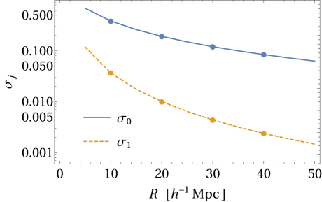
Figure 1: The values of $\sigma_{0}$ and $\sigma_{1}$ calculated from the perturbation theory (solid and dashed lines, respectively) and simulation data (points with error bars), as functions of smoothing radius $R$.

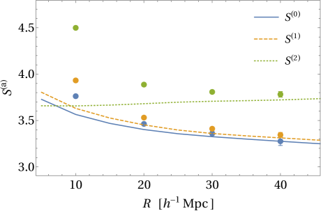
Figure 2: The values of skewness parameters $S^{(0)}$, $S^{(1)}$, $S^{(2)}$ calculated from the perturbation theory (solid, dashed and dotted lines, respectively) and simulation data (points with error bars), as functions of smoothing radius $R$.

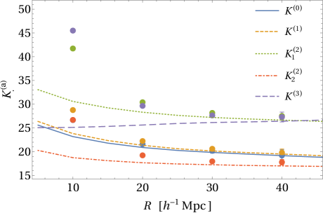
Figure 3: The values of kurtosis parameters $K^{(0)}$, $K^{(1)}$, $K^{(2)}_{1}$, $K^{(2)}_{2}$, $K^{(3)}$ calculated from the perturbation theory (solid, dashed, dotted, dash-dotted and long-dashed lines, respectively) and simulation data (points with error bars), as functions of smoothing radius $R$.

In Table 1, the parameters of the weakly non-Gaussian formula of Minkowski functionals are given. The upper figures of each entry represent the predictions of the lowest-order perturbation theory. The lower figures of each entry in Table 1 are the values calculated directly from the simulation data with Eqs. (10), (13)–(23). In Figures 1, 2 and 3, the values of various parameters calculated from the perturbation theory and simulation data are compared. The skewness and kurtosis parameters in the simulations are quantitatively reproduced by the tree-level perturbation theory on sufficiently large scales within 5% for $R\gtrsim 30\,h^{-1}\mathrm{Mpc}$, while the accuracy of the perturbation theory decreases to 10% for $R\sim 20\,h^{-1}\mathrm{Mpc}$ and much worse for $R\sim 10\,h^{-1}\mathrm{Mpc}$.

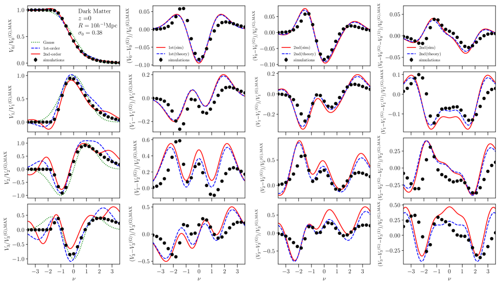
Figure 4: Minkowski functionals calculated from the numerical simulations (points with error bars) are compared with analytic formulas. A smoothing radius $R=10\,h^{-1}\mathrm{Mpc}$ is adopted. The panels in the leftmost row show the values of Minkowski functionals. The curves are normalized by the maximum of the absolute values for Gaussian predictions, $V_{k}^{\mathrm{(G),MAX}}$. The dotted lines correspond to the zeroth-order predictions, or Gaussian predictions, dashed lines correspond to the first-order predictions, and solid lines correspond to the second-order predictions. The parameter values for the first- and second-order predictions are numerically calculated from the simulations. The panels in the second and third rows show differences from the Gaussian predictions. The parameter values for the solid lines are taken from the numerical simulations, and those for the dashed lines are take from the predictions of the perturbation theory. In the panels in the second row, the analytic predictions with the first-order approximation are presented. In the panels in the third row, the analytic predictions with the second-order approximation are presented. In the panels in the rightmost row, differences from the first-order predictions are plotted.

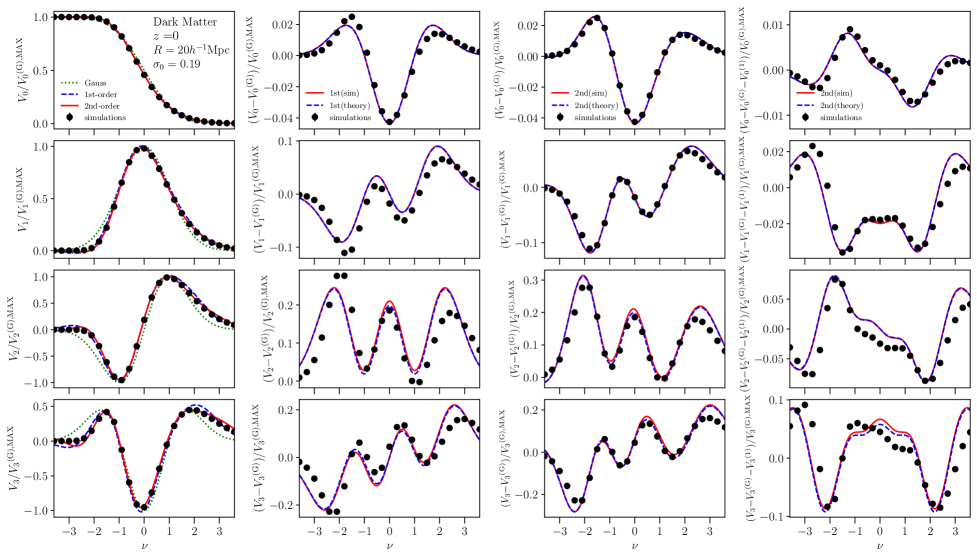
Figure 5: Same as Figure 4 but for the smoothing radius of $R=20\,h^{-1}\mathrm{Mpc}$.

Figure 6: Same as Figure 4 but for the smoothing radius of $R=30\,h^{-1}\mathrm{Mpc}$.

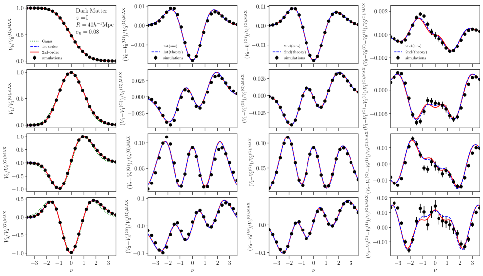
Figure 7: Same as Figure 4 but for the smoothing radius of $R=40\,h^{-1}\mathrm{Mpc}$.

Finally, the Minkowski functionals calculated from the numerical simulations are compared with analytic predictions in Figures 4–7. Each figure corresponds to different smoothing radius. The leftmost rows show the shape of the Minkowski functionals. The second and third rows show the differences from the Gaussian predictions, i.e., they depict the non-Gaussian effects. The lines in the second rows of the figures show the first-order corrections of non-Gaussianity in the analytic formula. The lines in the third rows of the figures show the second-order corrections of non-Gaussianity. The rightmost rows show the differences from the first-order predictions, i.e., they depict the second- and higher-order effects of non-Gaussianity in the Minkowski functionals.

As expected, the analytic predictions reproduce the results of numerical simulations when the smoothing radius is large and the expansion parameter $\sigma_{0}$ is small. The qualitative behaviors of the Minkowski functionals as functions the threshold are reproduced by the analytic formulas. Quantitatively, however, the agreements are better for large smoothing radii than for small smoothing radii, as expected. Comparing the second and third rows of each figure, the analytic formula with second-order corrections outperforms those with only first-order corrections. This shows the quantitative usefulness of taking the second-order effects into account. Purely second-order effects in the analytic formula are shown in the rightmost rows in the figures. For the smallest smoothing radius of $10\,h^{-1}\mathrm{Mpc}$, the performance of the analytic formula with parameters estimated from the perturbation theory and numerical simulations are similarly worse than the cases of larger smoothing radii. This means that the third- and higher-order corrections of the non-Gaussianity in the analytic formula are not negligible in the case of smallest smoothing radius.

V Conclusions

In this paper, we compare the second-order formula of weakly non-Gaussian Minkowski functionals to the results of $N$-body simulations of the large-scale structure. As expected, the nonlinear perturbation theory reproduces the deviations from the Gaussian predictions of Minkowski functionals when the smoothing radius is large enough. We quantitatively investigate the performance of the nonlinear perturbation theory against the numerical simulations.

The nonlinear perturbation theory predicts all the parameters in the analytic formula of weakly non-Gaussian Minkowski functionals. While the calculations of skewness and kurtosis parameters with the perturbation theory involve multi-dimensional integrals, parts of the integrations are analytically performed, and one can numerically evaluate all the necessary integrals without any difficulty. The predicted parameters are compared with those directly evaluated by the $N$-body simulations in Table 1 and Figures 1–3.

In our calculations, the nonlinear perturbation theory with tree-level approximations are adopted. Higher-order corrections of the perturbation theory with loop corrections may improve the theoretical predictions, while the numerical evaluations of the multi-dimensional integrals would be much harder. Investigations along this line is one of the possible extensions of the present work.

The Figures 4–7 show our comparisons of the Minkowski functionals between numerical results and analytical formula for various smoothing radius. As expected, the degree of agreement varies with smoothing radius. The analytic formula is better in the larger smoothing radius (i.e., smaller $\sigma_{0}$), as expected. While higher-order effects of both non-Gaussianity and the perturbation theory are simultaneously important for smaller smoothing radius, the analytic formula with larger smoothing radius outperforms the case of smaller smoothing radius.

In this paper, we only consider the clustering of dark matter in real space, and obviously ignore the effects of galaxy biasing and redshift-space distortions, which are inevitable in the actual observations of the large-scale structure of the Universe. While the purpose of this paper is to investigate the dynamically nonlinear effects on the Minkowski functionals of density fluctuations of dark matter, taking into account the biasing and redshift-space distortions should be necessary to realistically predict the shape of Minkowski functionals of observable galaxies. We will address these effects in future work.

Another important application of the present work (with extensions of including the observational effects mentioned above) is to see whether or not one can distinguish the primordial non-Gaussianity from the non-Gaussianity induced by nonlinear evolutions. The method developed in this paper should offer an analytic way of investigating this kind of issue in future work.

- (1) A. H. Guth, Phys. Rev. D23, 347 (1981).
- (2) K. Sato, Phys. Lett. 99B, 66 (1981).
- (3) A. D. Linde, Phys. Lett. B108, 389 (1982).
- (4) A. Albrecht and P. J. Steinhardt, Phys. Rev. Lett. 48, 1220 (1982).
- (5) J. Martin, C. Ringeval, and V. Vennin, Physics of the Dark Universe 5, 75 (2014).
- (6) P. J. E. Peebles, The Large-scale Structure of the Universe (Princeton, Princeton University Press, 1980).
- (7) Planck Collaboration, Y. Akrami, F. Arroja, et al., Astron. Astrophys. , 641, A9 (2020).
- (8) H. Minkowski, Mathematische Annalen 57, 447 (1903).
- (9) R. Schneider, Covex bodies: the Brunn-Minkowski theory (Cambridge University Press, Cambridge, 1993).
- (10) K. R. Mecke, T. Buchert, and H. Wagner, Astron. Astrophys. 288, 697 (1994).
- (11) J. Schmalzing and T. Buchert, Astrophys. J. Lett. 482, L1 (1997).
- (12) M. Kerscher, J. Schmalzing, J. Retzlaff, S. Borgani, T. Buchert, S. Gottlöber, V. Müller, M. Plionis, and H. Wagner, Mon. Not. R. Astron. Soc. 284, 73 (1997).
- (13) M. Kerscher, J. Schmalzing, T. Buchert, and H. Wagner, Astron. Astrophys. 333, 1 (1998).
- (14) V. Sahni, B. S. Sathyaprakash, and S. F. Shandarin, Astrophys. J. Lett. 495, L5 (1998).
- (15) J. Schmalzing, T. Buchert, A. L. Melott, V. Sahni, B. S. Sathyaprakash, and S. F. Shandarin, Astrophys. J. 526, 568 (1999).
- (16) M. Kerscher, K. Mecke, J. Schmalzing, C. Beisbart, T. Buchert, and H. Wagner, Astron. Astrophys. 373, 1 (2001).
- (17) J. V. Sheth, V. Sahni, S. F. Shandarin, and B. S. Sathyaprakash, Mon. Not. R. Astron. Soc. 343, 22 (2003).
- (18) C. Hikage, J. Schmalzing, T. Buchert, Y. Suto, I. Kayo, A. Taruya, M. S. Vogeley, F. Hoyle, J. R. Gott, and J. Brinkmann, Publ. Astron. Soc. Japan 55, 911 (2003).
- (19) S. F. Shandarin, J. V. Sheth, and V. Sahni, Mon. Not. R. Astron. Soc. 353, 162 (2004).
- (20) C. Hikage, E. Komatsu, and T. Matsubara, Astrophys. J. 653, 11 (2006).
- (21) M. Einasto, L. J. Liivamägi, E. Tempel, E. Saar, E. Tago, P. Einasto, I. Enkvist, J. Einasto, V. J. Martínez, P. Heinämäki, and P. Nurmi, Astrophys. J. 736, 51 (2011).
- (22) Y. Liu, Y. Yu, H.-R. Yu, and P. Zhang, Phys. Rev. D101, 063515 (2020).
- (23) H. Tomita, Progr. Theor. Phys., 76, 952 (1986).
- (24) T. Matsubara, Astrophys. J. Lett. 434, L43 (1994).
- (25) T. Matsubara, Astrophys. J. Suppl. Ser. 584, 1 (2003).
- (26) T. Matsubara, Phys. Rev. D81, 083505 (2010).
- (27) D. Pogosyan, C. Gay, and C. Pichon, Phys. Rev. D80, 081301 (2009); Phys. Rev. D81, 129901(E) (2010).
- (28) C. Gay, C. Pichon, and D. Pogosyan, Phys. Rev. D85, 023011 (2012).
- (29) S. Kuriki and T. Matsubara, [arXiv:2011.04953 [math.ST]].
- (30) T. Matsubara and S. Kuriki, [arXiv:2011.04954 [astro-ph.CO]].
- (31) F. Bernardeau, S. Colombi, E. Gaztañaga, and R. Scoccimarro, Physics Reports 367, 1 (2002).
- (32) M. H. Goroff, B. Grinstein, S.-J. Rey, et al., Astrophys. J. , 311, 6 (1986).
- (33) N. Makino, M. Sasaki, Y. Suto, Phys. Rev. D, 46, 585, (1992).
- (34) B. Jain and E. Bertschinger,Astrophys. J. , 431, 495 (1994).
- (35) E. L. Lokas, R. Juszkiewicz, D. H. Weinberg F. R. Bouchet, Mon. Not. R. Astron. Soc. , 274, 730 (1995).
- (36) F. Villaescusa-Navarro, C. Hahn, E. Massara, et al., Astrophys. J. Suppl. Ser. , 250, 2 (2020).
- (37) H. Hadwiger, Vorlesungen über Inhalt, Oberfläche und Isoperimetrie (Berlin, Springer, 1957).
- (38) M. W. Crofton, Philos. Trans. R. Soc. London, A158, 181 (1868)
- (39) J. Lesgourgues, arXiv:1104.2932.
- (40) D. Blas, J. Lesgourgues and T. Tram, J. Cosmol. Astropart. Phys. 07 (2011) 034.