A monolithic divergence-conforming HDG scheme for a linear fluid-structure interaction model

Abstract.

We present a novel monolithic divergence-conforming HDG scheme for a linear fluid-structure interaction (FSI) problem with a thick structure. A pressure-robust optimal energy-norm estimate is obtained for the semidiscrete scheme. When combined with a Crank-Nicolson time discretization, our fully discrete scheme is energy stable and produces an exactly divergence-free fluid velocity approximation. The resulting linear system, which is symmetric and indefinite, is solved using a preconditioned MinRes method with a robust block algebraic multigrid (AMG) preconditioner.

1. Introduction

Fluid-structure interaction (FSI) describes a multi-physics phenomenon that involves the highly non-linear coupling between a deformable or moving structure and a surrounding or internal fluid. There has been intensive interest in solving FSI problems due to its wide applications in biomedical, engineering and architecture fields, such as the simulation of blood-cell interactions, the study of wing fluttering in aerodynamics and the design of dams with reservoirs. However, it is generally difficult to achieve analytical solution to FSI problem with its nonlinear and multi-physics nature. Instead, there have been extensive studies in its numerical solutions and an increasing demand for more efficient and accurate numerical schemes [8, 12, 14, 26, 38].

Numerical methodologies for solving FSI problems can be roughly categorized into partitioned and monolithic schemes. Distinct mechanisms in fluid and structure domains naturally suggest solvers using partitioned schemes [17, 36]. This numerical procedure treats each physical phenomenon separately and allows the use of existing software frameworks that are well-established for each subproblem. However, the design of efficient partitioned schemes that produce stable and accurate results remains a challenge, especially when the density of fluid is comparable to that of structure due to numerical instabilities known as added mass effect [10]. The design and analysis of partitioned schemes to circumvent such problems has been an active research area in the past decade [10, 18, 32, 3, 6]. An alternative to partitioned strategy is the monolithic approach, which solves the fluid flow and structure dynamics simultaneously using one unified fully-coupled formulation [27, 43, 39]. The boundary conditions on the fluid-structure interface will be automatically satisfied in the procedure. Monolithic schemes are usually more robust than partitioned schemes and allow more rigorous analysis of discretization and solution techniques [29, 38]. However, monolithic schemes have been criticized for requiring well-designed preconditioners[23, 35, 2], more memory and computation time since the whole system is solved in one formulation.

In this paper, we present a novel monolithic divergence-conforming HDG scheme for a linear FSI problem with a thick structure. The fluid Stokes problem is discretized using the divergence-free HDG scheme of Lehrenfeld and Schöberl [30, 31], and the structure linear elasticity problem is discretized using the divergence-conforming HDG scheme of Fu et al. [22]. We approximate the fluid and structure velocities together using a single $H(\mathrm{div})$-conforming finite element space, and we also introduce a global (hybrid) unknown that approximate the tangential component of the velocities on the mesh skeleton for the purpose of efficient implementation. A pressure-robust optimal energy-norm estimate is obtained for the resulting semidiscrete scheme. We then use a Crank-Nicolson time discretization, and the fluid-structure interface conditions are naturally treated monolithically. Our fully discrete scheme produces an exactly divergence-free fluid velocity approximation and is energy stable.

When polynomials of degree $k\geq 1$ is used in the scheme, the global linear system, which is symmetric and indefinite, consists of degrees of freedom (DOFs) for the normal component of velocity (of polynomial degree $k$) on the mesh skeleton (facets), the tangential hybrid velocity (of polynomial degree $k-1$) on the mesh skeleton, and one pressure DOF per element on the mesh. The linear system problem is then solved via a preconditioned MinRes method [41] with a block diagonal preconditioner which is of similar form as the uniform preconditioner studied in Olshanskii et al. [37] for a generalized Stokes interface problem. We further use an auxiliary space preconditioner of Xu [44] with algebraic multigrid (AMG) for the velocity block and a hypre AMG preconditioner for the pressure block to arrive at the final block AMG preconditioner. This preconditioner is numerically verified to be robust with respect to mesh size, time step size, and material parameters.

The rest of the paper is organized as follows. In Section 2, we introduce the spatial and temporal discretization of the divergence-conforming HDG scheme for a linear FSI problem with a thick structure. We then present the block AMG preconditioner in Section 3. The a priori error analysis of the semidiscrete scheme is performed in Section 4. Numerical results are presented in Section 5. We conclude in Section 6.

2. The monolithic divergence-conforming HDG scheme for a linear FSI model

2.1. The model FSI problem

We consider the interaction between an incompressible, viscous fluid and a elastic structure. We denote by $\Omega^{f}(t)\subset\mathbb{R}^{d}$ the domain occupied by the fluid and $\Omega^{s}(t)\subset\mathbb{R}^{d}$, $d=2,3$ by the solid at the time $t\in[0,T]$. Let $\Gamma(t)=\overline{\Omega^{f}}\cap\overline{\Omega^{s}}$ be the part of the boundary where the elastic solid interacts with the fluid; see Fig. 1.

Figure 1. Sketch of a domain for FSI.

For the purpose of this paper, we assume that the nonlinear convection term in the fluid is negligible and the solid is linearly elastic and the deformation is small. Hence, the domain $\Omega^{f/s}$ does not change over time, and the fluid flow is modeled using the time dependent Stokes equations while the structure is modeled using the linear elastodynamics equations:

∇⋅𝒖f=0}\displaystyle\left.\begin{tabular}[]{rl}$\rho^{f}\partial_{t}\hbox{\boldmath$u$}^{f}-\nabla\cdot\hbox{\boldmath$\sigma$}^{f}(\hbox{\boldmath$u$}^{f},p^{f})=$&$\hbox{\boldmath$f$}^{f}$\\ $\nabla\cdot\hbox{\boldmath$u$}^{f}=$&$0$\end{tabular}\right\} ∂t𝜼s−𝒖s=0}\displaystyle\left.\begin{tabular}[]{rl}$\rho^{s}\partial_{t}\hbox{\boldmath$u$}^{s}-\nabla\cdot\hbox{\boldmath$\sigma$}^{s}(\hbox{\boldmath$\eta$}^{s})=$&$\hbox{\boldmath$f$}^{s}$\\ $\partial_{t}\hbox{\boldmath$\eta$}^{s}-\hbox{\boldmath$u$}^{s}=$&$0$\end{tabular}\right\}

(1c) =-ρf∂tuf⋅∇σf(uf,pf)ff $\displaystyle\;\;\text{in }\Omega^{f}\times[0,T],$

(1f) =-ρs∂tus⋅∇σs(ηs)fs $\displaystyle\;\;\text{in }\Omega^{s}\times[0,T],$

where $$\rho^{f} \hbox{\boldmath$u$}^{f} p^{f} \hbox{\boldmath$f$}^{f} \hbox{\boldmath$\sigma$}^{f}$$ is the fluid density, is the fluid velocity, is the fluid pressure, is the fluid source term, and is the fluid stress tensor given as follows:

$$\hbox{\boldmath$\sigma$}^{f}(\hbox{\boldmath$u$}^{f},p^{f}):=-p^{f}\hbox{\boldmath$I$}+2\mu^{f}\hbox{\boldmath$D$}(\hbox{\boldmath$u$}^{f}),$$

where $$I \mu^{f} \hbox{\boldmath$D$}(\hbox{\boldmath$u$}^{f}):=\frac{1}{2}(\nabla\hbox{\boldmath$u$}^{f}+(\nabla\hbox{\boldmath$u$}^{f})^{T}) \rho^{s} \hbox{\boldmath$\eta$}^{s} \hbox{\boldmath$u$}^{s} \hbox{\boldmath$f$}^{s} \hbox{\boldmath$\sigma$}^{s}$$ is the identity tensor, is the fluid viscosity, and is the fluid strain rate tensor, while is the structure density, is the structure displacement, is the structure velocity, is the structure source term, and is the structure Cauchy stress tensor given as follows:

$$\hbox{\boldmath$\sigma$}^{s}(\hbox{\boldmath$\eta$}^{s}):=\lambda^{s}(\nabla\cdot\hbox{\boldmath$\eta$}^{s})\hbox{\boldmath$I$}+2\mu^{s}\hbox{\boldmath$D$}(\hbox{\boldmath$\eta$}^{s}),$$

where $$\mu^{s} \lambda^{s}$$ and are the Lamé constants.

The fluid and structure sub-problems are coupled with the following kinematic and dynamic coupling conditions [38] on the interface $\Gamma$:

(1i) $$\left.\begin{tabular}[]{r}$\hbox{\boldmath$u$}^{f}=\;\hbox{\boldmath$u$}^{s}$\\ $\hbox{\boldmath$\sigma$}^{f}\hbox{\boldmath$n$}^{f}+\hbox{\boldmath$\sigma$}^{s}\hbox{\boldmath$n$}^{s}=\;0$\end{tabular}\right\}\text{ on }\Gamma\times[0,T],$$

where $\hbox{\boldmath$n$}^{f}$ and $\hbox{\boldmath$n$}^{s}$ are the normal directions on the fluid-structure interface $\Gamma$ pointing from the fluid and structure domains, respectively.

To close the system, we need proper initial and boundary conditions. For simplicity, in our analysis we consider a homogeneous Dirichlet boundary conditions on the exterior boundaries:

(1j) $$\hbox{\boldmath$u$}^{f}= \;0\;\;\text{ on }\Gamma^{f}:=\partial\Omega^{f}\backslash\Gamma,\quad\quad\hbox{\boldmath$\eta$}^{s}=\;0\;\;\text{ on }\Gamma^{s}:=\partial\Omega^{s}\backslash\Gamma.$$

We mention that other standard boundary conditions on the exterior boundaries can also be used, see e.g. the numerical results in Section 5. Finally, the initial condition is given as follows:

(1k) $$\hbox{\boldmath$u$}^{f}(x,0)= \;\hbox{\boldmath$u$}^{f}_{0}(x)\;\;\text{ on }\Omega^{f},\quad\quad\hbox{\boldmath$u$}^{s}(x,0)=\;\hbox{\boldmath$u$}^{s}_{0}(x),\,\hbox{\boldmath$\eta$}^{s}(x,0)=\;\hbox{\boldmath$\eta$}^{s}_{0}(x),\,\;\;\text{ on }\Omega^{s},$$

where $\hbox{\boldmath$u$}^{f}_{0},\hbox{\boldmath$u$}^{s}_{0}$, and $\hbox{\boldmath$\eta$}^{s}_{0}$, respectively, are the initial fluid velocity, initial structure velocity, and initial structure displacement, respectively.

2.2. Preliminaries and finite element spaces

We assume the domains $\Omega^{f}$, $\Omega^{s}$, as well as the interface $\Gamma$ are polypope. Let $\Omega$ be the union of the fluid and structure domains, i.e., $\overline{\Omega}=\overline{\Omega^{f}}\cup\overline{\Omega^{s}}$. Let $\mathcal{T}_{h}$ be an interface-fitted conforming simplicial triangulation of the domain $\Omega$ such that the interface $\Gamma$ is the union of element facets. For any element $K\in\mathcal{T}_{h}$, we denote by $h_{K}$ its diameter and we denote by $h$ the maximum diameter over all mesh elements. Denote by $\mathcal{T}_{h}^{f}$ the set of mesh elements that belong to $\Omega^{f}$ and by $\mathcal{T}_{h}^{s}$ those belong to $\Omega^{s}$. Denote by $\mathcal{E}_{h}$ the set of facets of $\mathcal{T}_{h}$, by $\mathcal{E}_{h}^{f}$ the set of facets that are interior to $\overline{\Omega^{f}}$, and by $\mathcal{E}_{h}^{s}$ the set of facets that are interior to $\overline{\Omega^{s}}$. We also denote by $\Gamma_{h}$, $\Gamma_{h}^{f}$, $\Gamma_{h}^{s}$ the set of facets that lie on the interface $\Gamma$, the fluid exterior boundary $\Gamma^{f}$, and the solid exterior boundary $\Gamma^{s}$, respectively. We have $\Gamma_{h}=\mathcal{E}_{h}^{f}\cap\mathcal{E}_{h}^{s}$. Given a simplex $S\subset\mathbb{R}^{d},d=1,2,3$, we denote $\mathcal{P}^{m}(S)$, $m\geq 0$, as the space of polynomials of degree at most $m$. Given a facet $F\in\mathcal{E}_{h}$ with normal direction $n$, we denote $\mathsf{tang}(\hbox{\boldmath$w$}):=\hbox{\boldmath$w$}-(\hbox{\boldmath$w$}\cdot\hbox{\boldmath$n$})\hbox{\boldmath$n$}$ as the tangential component of a vector field $w$.

The following finite element spaces will be used in our scheme:

(2a) $$\hbox{\boldmath$V$}_{h}^{r}:= \;\{\hbox{\boldmath$v$}\in H(\mathrm{div};\Omega):\;\;\hbox{\boldmath$v$}|_{K}\in[\mathcal{P}^{r}(K)]^{d},\;\forall K\in\mathcal{T}_{h}\},$$

(2b) $$\hbox{\boldmath$V$}_{h,0}^{r}:= \;\{\hbox{\boldmath$v$}\in\hbox{\boldmath$V$}_{h}^{r}:\;\;\hbox{\boldmath$v$}\cdot\hbox{\boldmath$n$}|_{F}=0,\;\forall F\in\Gamma_{h}^{f}\cup\Gamma_{h}^{s}\},$$

(2c) $$\widehat{\hbox{\boldmath$V$}}_{h}^{r}:= \;\{\widehat{\hbox{\boldmath$v$}}\in[L^{2}(\mathcal{E}_{h})]^{d}:\;\;\widehat{\hbox{\boldmath$v$}}|_{F}\in[\mathcal{P}^{r}(F)]^{d},\;\;\widehat{\hbox{\boldmath$v$}}\cdot\hbox{\boldmath$n$}|_{F}=0,\;\forall F\in\mathcal{E}_{h}\},$$

(2d) $$\widehat{\hbox{\boldmath$V$}}_{h,0}^{r}:= \;\{\widehat{\hbox{\boldmath$v$}}\in\widehat{\hbox{\boldmath$V$}}_{h}^{r,s}:\;\;\mathsf{tang}(\widehat{\hbox{\boldmath$v$}})|_{F}=0,\;\forall F\in\Gamma_{h}^{f}\cup\Gamma_{h}^{s}\},$$

(2e) $$Q_{h}^{r}:= \;\{q\in L^{2}(\Omega):\;\;q|_{K}\in\mathcal{P}^{r}(K),\;\forall K\in\mathcal{T}_{h}\},$$

where $$r\geq 0$$ is the polynomial degree.

We further use a superscript $f/s$ to indicate the restriction of these spaces on the fluid/structure domain, that is,

$$\hbox{\boldmath$V$}_{h,0}^{r,f}:=\{\hbox{\boldmath$v$}|_{\mathcal{T}_{h}^{f}}:\;\hbox{\boldmath$v$}\in\hbox{\boldmath$V$}_{h,0}^{r}\},\;\;\hbox{\boldmath$V$}_{h,0}^{r,s}:= \{\hbox{\boldmath$v$}|_{\mathcal{T}_{h}^{s}}:\;\hbox{\boldmath$v$}\in\hbox{\boldmath$V$}_{h,0}^{r}\},$$

$$\widehat{\hbox{\boldmath$V$}}_{h,0}^{r,f}:=\{\widehat{\hbox{\boldmath$v$}}|_{\mathcal{E}_{h}^{f}}:\;\widehat{\hbox{\boldmath$v$}}\in\widehat{\hbox{\boldmath$V$}}_{h,0}^{r}\},\;\;\widehat{\hbox{\boldmath$V$}}_{h,0}^{r,s}:= \{\widehat{\hbox{\boldmath$v$}}|_{\mathcal{E}_{h}^{s}}:\;\widehat{\hbox{\boldmath$v$}}\in\widehat{\hbox{\boldmath$V$}}_{h,0}^{r}\},$$

$$Q_{h}^{r,f}:=\{q|_{\mathcal{T}_{h}^{f}}:\;q\in Q_{h}^{r}\},\;\;Q_{h}^{r,s}:= \{q|_{\mathcal{T}_{h}^{s}}:\;q\in Q_{h}^{r}\}.$$

2.3. Semi-discrete divergence-conforming HDG scheme

In this subsection, we present the divergence-conforming HDG spatial discretization [30, 31, 22] of the linear FSI system (1).

We use the globally divergence-conforming finite element space $\hbox{\boldmath$V$}_{h}^{r}$ in (2b) to approximate the global velocity

(5) $$\hbox{\boldmath$u$}=\left\{\begin{tabular}[]{ll}$\hbox{\boldmath$u$}^{f}$&on $\Omega^{f}$,\\ $\hbox{\boldmath$u$}^{s}$&on $\Omega^{s}$\end{tabular}\right.,$$

and the global tangential facet finite element space $\widehat{\hbox{\boldmath$V$}}_{h}^{r}$ in (2d) to approximate the tangential component of the global velocity $u$ on the mesh skeleton.

The weak formulation of the divergence-conforming HDG scheme with polynomial degree $k\geq 1$ for (1) is given as follows: Find $(\hbox{\boldmath$u$}_{h},\widehat{\hbox{\boldmath$u$}}_{h},p_{h}^{f},\hbox{\boldmath$\eta$}_{h}^{s},\widehat{\hbox{\boldmath$\eta$}}_{h}^{s})\in\hbox{\boldmath$V$}_{h,0}^{k}\times\widehat{\hbox{\boldmath$V$}}_{h,0}^{k-1}\times Q_{h}^{k-1,f}\times\hbox{\boldmath$V$}_{h,0}^{k,s}\times\widehat{\hbox{\boldmath$V$}}_{h,0}^{k-1,s}$ such that

(6a) $$(\rho\partial_{t}\hbox{\boldmath$u$}_{h},\hbox{\boldmath$v$}_{h})+2\mu^{f}A_{h}^{f}((\hbox{\boldmath$u$}_{h},\widehat{\hbox{\boldmath$u$}}_{h}),(\hbox{\boldmath$v$}_{h},\widehat{\hbox{\boldmath$v$}}_{h}))-(p_{h}^{f},\nabla\cdot\hbox{\boldmath$v$}_{h})_{f}-(\nabla\cdot\hbox{\boldmath$u$}_{h},q_{h}^{f})_{f}\;\;$$

$$+2\mu^{s}A_{h}^{s}((\hbox{\boldmath$\eta$}^{s}_{h},\widehat{\hbox{\boldmath$\eta$}}^{s}_{h}),(\hbox{\boldmath$v$}_{h},\widehat{\hbox{\boldmath$v$}}_{h}))+\lambda^{s}(\nabla\cdot\hbox{\boldmath$\eta$}_{h}^{s},\nabla\cdot\hbox{\boldmath$v$}_{h})_{s} \;=\;(\hbox{\boldmath$f$},\hbox{\boldmath$v$}_{h}),$$

(6b) $$(\partial_{t}\hbox{\boldmath$\eta$}_{h}^{s}-\hbox{\boldmath$u$}_{h},\hbox{\boldmath$\xi$}_{h}^{s})_{s} \;=\;0,$$

(6c) $$\langle\partial_{t}\widehat{\hbox{\boldmath$\eta$}}_{h}^{s}-\widehat{\hbox{\boldmath$u$}}_{h},\widehat{\hbox{\boldmath$\xi$}}^{s}_{h}\rangle_{s} \;=\;0,$$

for all $$(\hbox{\boldmath$v$}_{h},\widehat{\hbox{\boldmath$v$}}_{h},q_{h}^{f},\hbox{\boldmath$\xi$}_{h}^{s},\widehat{\hbox{\boldmath$\xi$}}_{h}^{s})\in\hbox{\boldmath$V$}_{h,0}^{k}\times\widehat{\hbox{\boldmath$V$}}_{h,0}^{k-1}\times Q_{h}^{k-1,f}\times\hbox{\boldmath$V$}_{h,0}^{k,s}\times\widehat{\hbox{\boldmath$V$}}_{h,0}^{k-1,s} (\cdot,\cdot) L^{2} \Omega (\cdot,\cdot)_{f} L^{2} \Omega^{f} (\cdot,\cdot)_{s} L^{2} \Omega^{s} \langle\cdot,\cdot\rangle_{s} L^{2}(\mathcal{E}_{h}^{s}) \mathcal{E}_{h}^{s} \rho=\left\{\begin{tabular}[]{ll}$\rho^{f}$&on $\Omega^{f}$\\ $\rho^{s}$&on $\Omega^{s}$\end{tabular}\right. \hbox{\boldmath$f$}=\left\{\begin{tabular}[]{ll}$\hbox{\boldmath$f$}^{f}$&on $\Omega^{f}$\\ $\hbox{\boldmath$f$}^{s}$&on $\Omega^{s}$\end{tabular}\right. \Omega A_{h}^{f} A_{h}^{s} i\in\{f,s\}$$, where denotes the -inner product on the domain , denotes the -inner product on the fluid domain , denotes the -inner product on the structure domain , and denotes the -inner product on the structure mesh skeleton , moreover, is the global density and is the global source term on . Here the operators and are the following symmetric interior penalty HDG diffusion operators with a projected jumps formulation: for ,

(7) $$A_{h}^{i}((\hbox{\boldmath$v$}_{h},\widehat{\hbox{\boldmath$v$}}_{h}),(\hbox{\boldmath$w$}_{h},\widehat{\hbox{\boldmath$w$}}_{h})):=\sum_{K\in\mathcal{T}_{h}^{i}} \;\int_{K}\hbox{\boldmath$D$}(\hbox{\boldmath$v$}_{h}):\hbox{\boldmath$D$}(\hbox{\boldmath$w$}_{h})\,\mathrm{dx}-\int_{\partial K}\hbox{\boldmath$D$}(\hbox{\boldmath$v$}_{h})\hbox{\boldmath$n$}\cdot\mathsf{tang}(\hbox{\boldmath$w$}_{h}-\widehat{\hbox{\boldmath$w$}}_{h})\,\mathrm{ds}$$

$$-\int_{\partial K}\hbox{\boldmath$D$}(\hbox{\boldmath$w$}_{h})\hbox{\boldmath$n$}\cdot\mathsf{tang}(\hbox{\boldmath$v$}_{h}-\widehat{\hbox{\boldmath$v$}}_{h})\,\mathrm{ds}+\int_{\partial K}\frac{\alpha k^{2}}{h}\Pi_{h}(\mathsf{tang}(\hbox{\boldmath$v$}_{h}-\widehat{\hbox{\boldmath$v$}}_{h}))\cdot\Pi_{h}(\mathsf{tang}(\hbox{\boldmath$w$}_{h}-\widehat{\hbox{\boldmath$w$}}_{h}))\,\mathrm{ds},$$

where $\Pi_{h}$ denotes the $L^{2}(\mathcal{E}_{h})$-projection onto the tangential facet finite element space $\widehat{\hbox{\boldmath$V$}}_{h}^{k-1}$. Efficient implementation of this local projector $\Pi_{h}$ was discussed in [31, Section 2.2.2]. Here $\alpha>0$ is a sufficiently large stabilization parameter that ensures the following coercivity result:

(8) $$A_{h}^{i}((\hbox{\boldmath$v$}_{h},\widehat{\hbox{\boldmath$v$}}_{h}),(\hbox{\boldmath$v$}_{h},\widehat{\hbox{\boldmath$v$}}_{h}))\geq\frac{1}{2}\sum_{K\in\mathcal{T}_{h}^{i}}\left(\|\hbox{\boldmath$D$}(\hbox{\boldmath$v$}_{h})\|_{K}^{2}+\frac{\alpha k^{2}}{h}\|\Pi_{h}(\mathsf{tang}(\hbox{\boldmath$v$}_{h}-\widehat{\hbox{\boldmath$v$}}_{h}))\|_{\partial K}^{2}\right),$$

where $\|\cdot\|_{S}$ indicates the $L^{2}$-norm on the domain $S$. A sufficient condition on $\alpha$ that guarantees the above coercivity result was presented in [1, Lemma 1]. We take $\alpha=8$ in our numerical experiments in Section 5.

The following two results show consistency and stability of the semi-discrete scheme (6).

Lemma 2.1 (Galerkin-orthogonality for the semi-discrete scheme).

Let $(\hbox{\boldmath$u$},p^{f},\hbox{\boldmath$\eta$}^{s})\in H^{2}(\Omega)\times H^{1}(\Omega^{f})\times H^{2}(\Omega^{s})$ be the solution to the model problem (1). Then, the equations (6) holds true with $(\hbox{\boldmath$u$}_{h},\widehat{\hbox{\boldmath$u$}}_{h},p^{f}_{h},\hbox{\boldmath$\eta$}^{s}_{h},\widehat{\hbox{\boldmath$\eta$}}^{s}_{h})$ replaced by $(\hbox{\boldmath$u$},\hbox{\boldmath$u$}|_{\mathcal{E}_{h}},p^{f},\hbox{\boldmath$\eta$}^{s},\hbox{\boldmath$\eta$}^{s}|_{\mathcal{E}_{h}^{s}})$. That is, we have

(9a) $$(\rho\partial_{t}\hbox{\boldmath$u$},\hbox{\boldmath$v$}_{h})+2\mu^{f}A_{h}^{f}((\hbox{\boldmath$u$},\widehat{\hbox{\boldmath$u$}}),(\hbox{\boldmath$v$}_{h},\widehat{\hbox{\boldmath$v$}}_{h}))-(p^{f},\nabla\cdot\hbox{\boldmath$v$}_{h})_{f}-(\nabla\cdot\hbox{\boldmath$u$},q_{h}^{f})_{f}\;\;$$

$$+2\mu^{s}A_{h}^{s}((\hbox{\boldmath$\eta$}^{s},\widehat{\hbox{\boldmath$\eta$}}^{s}),(\hbox{\boldmath$v$}_{h},\widehat{\hbox{\boldmath$v$}}_{h}))+\lambda^{s}(\nabla\cdot\hbox{\boldmath$\eta$}^{s},\nabla\cdot\hbox{\boldmath$v$}_{h})_{s} \;=\;(\hbox{\boldmath$f$},\hbox{\boldmath$v$}_{h}),$$

(9b) $$(\partial_{t}\hbox{\boldmath$\eta$}^{s}-\hbox{\boldmath$u$},\hbox{\boldmath$\xi$}_{h}^{s})_{s} \;=\;0,$$

(9c) $$\langle\partial_{t}\widehat{\hbox{\boldmath$\eta$}}^{s}-\widehat{\hbox{\boldmath$u$}},\widehat{\hbox{\boldmath$\xi$}}^{s}_{h}\rangle_{s} \;=\;0,$$

for all $$(\hbox{\boldmath$v$}_{h},\widehat{\hbox{\boldmath$v$}}_{h},q_{h}^{f},\hbox{\boldmath$\xi$}_{h}^{s},\widehat{\hbox{\boldmath$\xi$}}_{h}^{s})\in\hbox{\boldmath$V$}_{h,0}^{k}\times\widehat{\hbox{\boldmath$V$}}_{h,0}^{k-1}\times Q_{h}^{k-1,f}\times\hbox{\boldmath$V$}_{h,0}^{k,s}\times\widehat{\hbox{\boldmath$V$}}_{h,0}^{k-1,s} \widehat{\hbox{\boldmath$u$}}=\hbox{\boldmath$u$}|_{\mathcal{E}_{h}} \widehat{\hbox{\boldmath$\eta$}}^{s}=\hbox{\boldmath$\eta$}^{s}|_{\mathcal{E}_{h}^{s}}$$, where and .

Proof.

The equations (9b) and (9c) follows from the second equation in (1f). We are left to prove the equation (9a). Since $\mathsf{tang}(\hbox{\boldmath$u$}-\widehat{\hbox{\boldmath$u$}})=0$, we have, for any function $(\hbox{\boldmath$v$}_{h},\widehat{\hbox{\boldmath$v$}}_{h})\in\hbox{\boldmath$V$}_{h,0}^{k}\times\widehat{\hbox{\boldmath$V$}}_{h,0}^{k-1}$,

$$A_{h}^{f}((\hbox{\boldmath$u$},\widehat{\hbox{\boldmath$u$}}),(\hbox{\boldmath$v$}_{h},\widehat{\hbox{\boldmath$v$}}_{h}))= \;\sum_{K\in\mathcal{T}_{h}^{f}}\;\int_{K}\hbox{\boldmath$D$}(\hbox{\boldmath$u$}):\hbox{\boldmath$D$}(\hbox{\boldmath$v$}_{h})\,\mathrm{dx}-\int_{\partial K}\hbox{\boldmath$D$}(\hbox{\boldmath$u$})\hbox{\boldmath$n$}\cdot\mathsf{tang}(\hbox{\boldmath$v$}_{h}-\widehat{\hbox{\boldmath$v$}}_{h})\,\mathrm{ds}$$

$$= \;-(\nabla\cdot\hbox{\boldmath$D$}(\hbox{\boldmath$u$}),\hbox{\boldmath$v$}_{h})_{f}+\sum_{K\in\mathcal{T}_{h}^{f}}\int_{\partial K}\hbox{\boldmath$D$}(\hbox{\boldmath$u$})\hbox{\boldmath$n$}\cdot((\hbox{\boldmath$v$}_{h}\cdot\hbox{\boldmath$n$})\hbox{\boldmath$n$}+\mathsf{tang}(\widehat{\hbox{\boldmath$v$}}_{h}))\,\mathrm{ds}$$

$$= \;-(\nabla\cdot\hbox{\boldmath$D$}(\hbox{\boldmath$u$}),\hbox{\boldmath$v$}_{h})_{f}+\int_{\Gamma_{h}}\hbox{\boldmath$D$}(\hbox{\boldmath$u$})\hbox{\boldmath$n$}^{f}\cdot((\hbox{\boldmath$v$}_{h}\cdot\hbox{\boldmath$n$})\hbox{\boldmath$n$}+\mathsf{tang}(\widehat{\hbox{\boldmath$v$}}_{h}))\,\mathrm{ds}.$$

Similarly, we have, for any function $(\hbox{\boldmath$v$}_{h},\widehat{\hbox{\boldmath$v$}}_{h})\in\hbox{\boldmath$V$}_{h,0}^{k}\times\widehat{\hbox{\boldmath$V$}}_{h,0}^{k-1}$,

$$A_{h}^{s}((\hbox{\boldmath$\eta$}^{s},\widehat{\hbox{\boldmath$\eta$}^{s}}),(\hbox{\boldmath$v$}_{h},\widehat{\hbox{\boldmath$v$}}_{h}))= \;-(\nabla\cdot\hbox{\boldmath$D$}(\hbox{\boldmath$\eta$}^{s}),\hbox{\boldmath$v$}_{h})_{s}+\int_{\Gamma_{h}}\hbox{\boldmath$D$}(\hbox{\boldmath$\eta$}^{s})\hbox{\boldmath$n$}^{s}\cdot((\hbox{\boldmath$v$}_{h}\cdot\hbox{\boldmath$n$})\hbox{\boldmath$n$}+\mathsf{tang}(\widehat{\hbox{\boldmath$v$}}_{h}))\,\mathrm{ds},$$

$$(p^{f},\nabla\cdot\hbox{\boldmath$v$}_{h})_{f}= \;-(\nabla p^{f},\hbox{\boldmath$v$}_{h})_{f}+\int_{\Gamma_{h}}p^{f}(\hbox{\boldmath$v$}_{h}\cdot\hbox{\boldmath$n$}^{f})\,\mathrm{ds},$$

$$(\nabla\cdot\hbox{\boldmath$\eta$}^{s},\nabla\cdot\hbox{\boldmath$v$}_{h})_{s}= \;-(\nabla(\nabla\cdot\hbox{\boldmath$\eta$}^{s}),\hbox{\boldmath$v$}_{h})_{s}+\int_{\Gamma_{h}}(\nabla\cdot\hbox{\boldmath$\eta$}^{s})(\hbox{\boldmath$v$}_{h}\cdot\hbox{\boldmath$n$}^{s})\,\mathrm{ds}.$$

Combining these equations, we get

$$(\rho\partial_{t}\hbox{\boldmath$u$},\hbox{\boldmath$v$}_{h})+2\mu^{f}A_{h}^{f}((\hbox{\boldmath$u$},\widehat{\hbox{\boldmath$u$}}),(\hbox{\boldmath$v$}_{h},\widehat{\hbox{\boldmath$v$}}_{h}))-(p^{f},\nabla\cdot\hbox{\boldmath$v$}_{h})_{f}-(\nabla\cdot\hbox{\boldmath$u$},q_{h}^{f})_{f}\;\;$$

$$+2\mu^{s}A_{h}^{s}((\hbox{\boldmath$\eta$}^{s},\widehat{\hbox{\boldmath$\eta$}}^{s}),(\hbox{\boldmath$v$}_{h},\widehat{\hbox{\boldmath$v$}}_{h}))+\lambda^{s}(\nabla\cdot\hbox{\boldmath$\eta$}^{s},\nabla\cdot\hbox{\boldmath$v$}_{h})_{s}-(\hbox{\boldmath$f$},\hbox{\boldmath$v$}_{h})\;$$

$$=\;(\rho^{f}\partial_{t}\hbox{\boldmath$u$}^{f}-\nabla\cdot\hbox{\boldmath$\sigma$}^{f}-\hbox{\boldmath$f$}^{f},\hbox{\boldmath$v$}_{h})_{f}+(\rho^{s}\partial_{t}\hbox{\boldmath$u$}^{s}-\nabla\cdot\hbox{\boldmath$\sigma$}^{s}-\hbox{\boldmath$f$}^{s},\hbox{\boldmath$v$}_{h})_{s}$$

$$\;\;\;\;+\int_{\Gamma_{h}}(\hbox{\boldmath$\sigma$}^{f}\hbox{\boldmath$n$}^{f}+\hbox{\boldmath$\sigma$}^{s}\hbox{\boldmath$n$}^{s})((\hbox{\boldmath$v$}_{h}\cdot\hbox{\boldmath$n$})\cdot\hbox{\boldmath$n$}+\mathsf{tang}(\widehat{\hbox{\boldmath$v$}}_{h})))\,\mathrm{ds}$$

$$=0,$$

where we used the PDE (1c), (1f), and the dynamic interface condition in (1i). This completes the proof of the equation $\eqref{semiX-1}$. ∎

Lemma 2.2 (Stability for the semi-discrete scheme).

Let $(\hbox{\boldmath$u$}_{h},\widehat{\hbox{\boldmath$u$}}_{h},p_{h}^{f},\hbox{\boldmath$\eta$}_{h}^{s},\widehat{\hbox{\boldmath$\eta$}}_{h}^{s})\in\hbox{\boldmath$V$}_{h,0}^{k}\times\widehat{\hbox{\boldmath$V$}}_{h,0}^{k-1}\times Q_{h}^{k-1,f}\times\hbox{\boldmath$V$}_{h,0}^{k,s}\times\widehat{\hbox{\boldmath$V$}}_{h,0}^{k-1,s}$ be the numerical solution to the semi-discrete scheme (6). Then, the velocity approximation on the fluid domain is exactly divergence free:

(10) $$\nabla\cdot\hbox{\boldmath$u$}_{h}|_{\mathcal{T}_{h}^{f}}=0,$$

and the following energy identity holds:

(11) $$\frac{1}{2}\frac{d}{dt}E_{h}=-2\mu^{f}A_{h}^{f}((\hbox{\boldmath$u$}_{h},\widehat{\hbox{\boldmath$u$}}_{h}),(\hbox{\boldmath$u$}_{h},\widehat{\hbox{\boldmath$u$}}_{h}))+(\hbox{\boldmath$f$},\hbox{\boldmath$u$}_{h}),$$

where $E_{h}:=(\rho\hbox{\boldmath$u$}_{h},\hbox{\boldmath$u$}_{h})+\lambda^{s}(\nabla\cdot\hbox{\boldmath$\eta$}_{h}^{s},\nabla\cdot\hbox{\boldmath$\eta$}^{s}_{h})_{s}+2\mu^{s}A_{h}^{s}((\hbox{\boldmath$\eta$}_{h},\widehat{\hbox{\boldmath$\eta$}}_{h}),(\hbox{\boldmath$\eta$}_{h},\widehat{\hbox{\boldmath$\eta$}}_{h}))$ is the total energy.

Proof.

Let us first prove the divergence-free property (10). By the choice of the velocity finite element space $\hbox{\boldmath$V$}_{h}^{k}$ and fluid pressure finite element space $Q_{h}^{k-1,f}$, we have $\nabla\cdot\hbox{\boldmath$u$}_{h}|_{\mathcal{T}_{h}^{f}}\in Q_{h}^{k-1,f}$. Now taking $q_{h}^{f}=\nabla\cdot\hbox{\boldmath$u$}_{h}|_{\mathcal{T}_{h}^{f}}$ in equation (6a), we get

$$(\nabla\cdot\hbox{\boldmath$u$}_{h},\nabla\cdot\hbox{\boldmath$u$}_{h})_{f}=0.$$

Hence the divergence-free property (10) holds true.

Next, let us prove the energy identity (11). Taking test function $(\hbox{\boldmath$v$}_{h},\widehat{\hbox{\boldmath$v$}}_{h})=(\hbox{\boldmath$u$}_{h},\widehat{\hbox{\boldmath$u$}}_{h})$ in equation (6a), and using the divergence-free property (10), we get

$$(\rho\partial_{t}\hbox{\boldmath$u$}_{h},\hbox{\boldmath$u$}_{h})+2\mu^{f}A_{h}^{f}((\hbox{\boldmath$u$}_{h},\widehat{\hbox{\boldmath$u$}}_{h}),(\hbox{\boldmath$u$}_{h},\widehat{\hbox{\boldmath$u$}}_{h}))+2\mu^{s}A_{h}^{s}((\hbox{\boldmath$\eta$}^{s}_{h},\widehat{\hbox{\boldmath$\eta$}}^{s}_{h}),(\hbox{\boldmath$u$}_{h},\widehat{\hbox{\boldmath$u$}}_{h}))+\lambda^{s}(\nabla\cdot\hbox{\boldmath$\eta$}_{h}^{s},\nabla\cdot\hbox{\boldmath$u$}_{h})_{s} \;=\;(\hbox{\boldmath$f$},\hbox{\boldmath$v$}_{h}).$$

Since $\hbox{\boldmath$u$}_{h}|_{\mathcal{T}_{h}^{s}}\in\hbox{\boldmath$V$}_{h}^{k,s}$ and $\widehat{\hbox{\boldmath$u$}}_{h}|_{\mathcal{E}_{h}^{s}}\in\widehat{\hbox{\boldmath$V$}}_{h}^{k-1,s}$, equations (6b)–(6c) implies that

$$\hbox{\boldmath$u$}_{h}|_{\mathcal{T}_{h}^{s}}=\partial_{t}\hbox{\boldmath$\eta$}_{h}^{s},\text{ and }\widehat{\hbox{\boldmath$u$}}_{h}|_{\mathcal{E}_{h}^{s}}=\partial_{t}{\widehat{\hbox{\boldmath$\eta$}}}_{h}^{s}.$$

Hence,

$$2\mu^{s}A_{h}^{s}((\hbox{\boldmath$\eta$}^{s}_{h},\widehat{\hbox{\boldmath$\eta$}}^{s}_{h}),(\hbox{\boldmath$u$}_{h},\widehat{\hbox{\boldmath$u$}}_{h}))=2\mu^{s}A_{h}^{s}((\hbox{\boldmath$\eta$}^{s}_{h},\widehat{\hbox{\boldmath$\eta$}}^{s}_{h}),(\partial_{t}\hbox{\boldmath$\eta$}^{s}_{h},\partial_{t}\widehat{\hbox{\boldmath$\eta$}}_{h}^{s}))=\frac{1}{2}\frac{d}{dt}(2\mu^{s}A_{h}^{s}((\hbox{\boldmath$\eta$}^{s}_{h},\widehat{\hbox{\boldmath$\eta$}}^{s}_{h}),(\hbox{\boldmath$\eta$}^{s}_{h},\widehat{\hbox{\boldmath$\eta$}}_{h}^{s}))),$$

and

$$\lambda^{s}(\nabla\cdot\hbox{\boldmath$\eta$}_{h}^{s},\nabla\cdot\hbox{\boldmath$u$}_{h})_{s}=\frac{1}{2}\frac{d}{dt}\left(\lambda^{s}(\nabla\cdot\hbox{\boldmath$\eta$}_{h}^{s},\nabla\cdot\hbox{\boldmath$\eta$}_{h}^{s})_{s}\right).$$

Combining the above equations, we arrive at the energy identity (11). This completes the proof. ∎

2.4. Monolithlic fully discrete divergence-conforming HDG scheme

In this subsection, we consider the temporal discretization of the semi-discrete scheme (6). We propose to use the second-order Crank-Nicolson scheme. For any positive integer $j\in\mathbb{Z}_{+}$, let $(\hbox{\boldmath$u$}_{h}^{j-1},\hbox{\boldmath$\eta$}_{h}^{s,j-1},\widehat{\hbox{\boldmath$\eta$}}_{h}^{s,j-1})\in\hbox{\boldmath$V$}_{h,0}^{k}\times\hbox{\boldmath$V$}_{h,0}^{k,s}\times\widehat{\hbox{\boldmath$V$}}_{h,0}^{k-1,s}$ be the numerical solution at time $t_{j-1}$. Give the time step size $\delta t_{j-1}>0$, we proceed to find the solution $(\hbox{\boldmath$u$}_{h}^{j},\hbox{\boldmath$\eta$}_{h}^{s,j},\widehat{\hbox{\boldmath$\eta$}}_{h}^{s,j})\in\hbox{\boldmath$V$}_{h,0}^{k}\times\hbox{\boldmath$V$}_{h,0}^{k,s}\times\widehat{\hbox{\boldmath$V$}}_{h,0}^{k-1,s}$ at time $t_{j}=t_{j-1}+\delta t_{j-1}$ along with the solution $(\widehat{\hbox{\boldmath$u$}}_{h}^{j-1/2},p_{h}^{f,j-1/2})\in\widehat{\hbox{\boldmath$V$}}_{h,0}^{k-1}\times Q_{h}^{k-1,f}$ at time $t_{j-1/2}=t_{j-1}+\frac{1}{2}\delta t_{j-1}$ such that the following equations holds:

(12a) $$(\rho\frac{\hbox{\boldmath$u$}_{h}^{j}-\hbox{\boldmath$u$}_{h}^{j-1}}{\delta t_{j-1}},\hbox{\boldmath$v$}_{h})+2\mu^{f}A_{h}^{f}((\hbox{\boldmath$u$}_{h}^{j-1/2},\widehat{\hbox{\boldmath$u$}}_{h}^{j-1/2}),(\hbox{\boldmath$v$}_{h},\widehat{\hbox{\boldmath$v$}}_{h}))-(p_{h}^{f,j-1/2},\nabla\cdot\hbox{\boldmath$v$}_{h})_{f}$$

$$\;\;-(\nabla\cdot\hbox{\boldmath$u$}_{h}^{j-1/2},q_{h}^{f})_{f}\;\;+2\mu^{s}A_{h}^{s}((\hbox{\boldmath$\eta$}^{s,j-1/2}_{h},\widehat{\hbox{\boldmath$\eta$}}^{s,j-1/2}_{h}),(\hbox{\boldmath$v$}_{h},\widehat{\hbox{\boldmath$v$}}_{h}))+\lambda^{s}(\nabla\cdot\hbox{\boldmath$\eta$}_{h}^{s,j-1/2},\nabla\cdot\hbox{\boldmath$v$}_{h})_{s} \;=\;(\hbox{\boldmath$f$}^{j-1/2},\hbox{\boldmath$v$}_{h}),$$

(12b) $$(\frac{\hbox{\boldmath$\eta$}_{h}^{s,j}-\hbox{\boldmath$\eta$}_{h}^{s,j-1}}{\delta t_{j-1}}-\hbox{\boldmath$u$}_{h}^{j-1/2},\hbox{\boldmath$\xi$}_{h}^{s})_{s} \;=\;0,$$

(12c) $$\langle\frac{\widehat{\hbox{\boldmath$\eta$}}_{h}^{s,j}-\widehat{\hbox{\boldmath$\eta$}}_{h}^{s,j-1}}{\delta t_{j-1}}-\widehat{\hbox{\boldmath$u$}}_{h}^{j-1/2},\widehat{\hbox{\boldmath$\xi$}}^{s}_{h}\rangle_{s} \;=\;0,$$

for all $$(\hbox{\boldmath$v$}_{h},\widehat{\hbox{\boldmath$v$}}_{h},q_{h}^{f},\hbox{\boldmath$\xi$}_{h}^{s},\widehat{\hbox{\boldmath$\xi$}}_{h}^{s})\in\hbox{\boldmath$V$}_{h,0}^{k}\times\widehat{\hbox{\boldmath$V$}}_{h,0}^{k-1}\times Q_{h}^{k-1,f}\times\hbox{\boldmath$V$}_{h,0}^{k,s}\times\widehat{\hbox{\boldmath$V$}}_{h,0}^{k-1,s}$$, where

$$\hbox{\boldmath$u$}_{h}^{j-1/2}:=\frac{1}{2}(\hbox{\boldmath$u$}_{h}^{j}+\hbox{\boldmath$u$}_{h}^{j-1}),\;\;\hbox{\boldmath$\eta$}_{h}^{s,j-1/2}:=\frac{1}{2}(\hbox{\boldmath$\eta$}_{h}^{s,j}+\hbox{\boldmath$\eta$}_{h}^{s,j-1}),\;\;\widehat{\hbox{\boldmath$\eta$}}_{h}^{s,j-1/2}:=\frac{1}{2}(\widehat{\hbox{\boldmath$\eta$}}_{h}^{s,j}+\widehat{\hbox{\boldmath$\eta$}}_{h}^{s,j-1}),$$

We have the following result on the energy stability of the fully discrete scheme (12).

Lemma 2.3 (Stability for the fully discrete scheme).

Let $(\hbox{\boldmath$u$}_{h}^{0},\hbox{\boldmath$\eta$}_{h}^{s,0},\widehat{\hbox{\boldmath$\eta$}}_{h}^{s,0})\in\hbox{\boldmath$V$}_{h,0}^{k}\times\hbox{\boldmath$V$}_{h,0}^{k,s}\times\widehat{\hbox{\boldmath$V$}}_{h,0}^{k-1,s}$ be a proper projection of the initial data in (1k) such that $\nabla\cdot\hbox{\boldmath$u$}_{h}^{0}|_{\mathcal{T}_{h}^{f}}=0$. For any positive integer $j\in\mathbb{Z}_{+}$, let $(\hbox{\boldmath$u$}_{h}^{j},\widehat{\hbox{\boldmath$u$}}_{h}^{j-1/2},p_{h}^{f,j-1/2},\hbox{\boldmath$\eta$}_{h}^{s,j},\widehat{\hbox{\boldmath$\eta$}}_{h}^{s,j})\in\hbox{\boldmath$V$}_{h,0}^{k}\times\widehat{\hbox{\boldmath$V$}}_{h,0}^{k-1}\times Q_{h}^{k-1,f}\times\hbox{\boldmath$V$}_{h,0}^{k,s}\times\widehat{\hbox{\boldmath$V$}}_{h,0}^{k-1,s}$ be the numerical solution to the fully discrete scheme (12). Then, the velocity approximation on the fluid domain is exactly divergence free:

(13) $$\nabla\cdot\hbox{\boldmath$u$}_{h}^{j}|_{\mathcal{T}_{h}^{f}}=0,$$

and the following energy identity holds true:

(14) $$\frac{1}{2}\frac{E_{h}^{j}-E_{h}^{j-1}}{\delta t_{j-1}}=-2\mu^{f}A_{h}^{f}((\hbox{\boldmath$u$}_{h}^{j-1/2},\widehat{\hbox{\boldmath$u$}}_{h}^{j-1/2}),(\hbox{\boldmath$u$}_{h}^{j-1/2},\widehat{\hbox{\boldmath$u$}}_{h}^{j-1/2}))+(\hbox{\boldmath$f$}^{j-1/2},\hbox{\boldmath$u$}_{h}),$$

where $E_{h}^{j}:=(\rho\hbox{\boldmath$u$}_{h}^{j},\hbox{\boldmath$u$}_{h}^{j})+\lambda^{s}(\nabla\cdot\hbox{\boldmath$\eta$}_{h}^{s,j},\nabla\cdot\hbox{\boldmath$\eta$}^{s,j}_{h})_{s}+2\mu^{s}A_{h}^{s}((\hbox{\boldmath$\eta$}^{s,j}_{h},\widehat{\hbox{\boldmath$\eta$}}^{s,j}_{h}),(\hbox{\boldmath$\eta$}^{s,j}_{h},\widehat{\hbox{\boldmath$\eta$}}^{s,j}_{h}))$ is the total energy at time $t_{j}$.

Proof.

The proof follows the same line as those for the semi-discrete case in Lemma 2.2, which we omit for simplicity. ∎

2.4.1. Efficient implementation of the fully discrete scheme (12)

We now present an efficient implementation of the scheme (12) whose globally coupled linear system consists of DOFs for the normal component of the velocity approximation, the tangential component of the hybrid velocity approximation on the mesh skeleton, and one pressure DOF per element on the mesh.

We need the following result on the characterization of the fully discrete solution.

Lemma 2.4 (Characterization of the fully discrete solution).

For any positive integer $$j\in\mathbb{Z}_{+} (\hbox{\boldmath$u$}_{h}^{j},\widehat{\hbox{\boldmath$u$}}_{h}^{j-1/2},p_{h}^{f,j-1/2},\hbox{\boldmath$\eta$}_{h}^{s,j},\widehat{\hbox{\boldmath$\eta$}}_{h}^{s,j})\in\hbox{\boldmath$V$}_{h,0}^{k}\times\widehat{\hbox{\boldmath$V$}}_{h,0}^{k-1}\times Q_{h}^{k-1,f}\times\hbox{\boldmath$V$}_{h,0}^{k,s}\times\widehat{\hbox{\boldmath$V$}}_{h,0}^{k-1,s} (\hbox{\boldmath$u$}_{h}^{j-1/2},\widehat{\hbox{\boldmath$u$}}_{h}^{j-1/2},p_{h}^{f,j-1/2})\in\hbox{\boldmath$V$}_{h,0}^{k}\times\widehat{\hbox{\boldmath$V$}}_{h,0}^{k-1}\times Q_{h}^{k-1,f}$$, let be the numerical solution to the fully discrete scheme (12). Then, is the unique solution to the following equations:

(15a) $$(2\rho\frac{\hbox{\boldmath$u$}_{h}^{j-1/2}}{\delta t_{j-1}},\hbox{\boldmath$v$}_{h})+2\mu^{f}A_{h}^{f}((\hbox{\boldmath$u$}_{h}^{j-1/2},\widehat{\hbox{\boldmath$u$}}_{h}^{j-1/2}),(\hbox{\boldmath$v$}_{h},\widehat{\hbox{\boldmath$v$}}_{h}))$$

$$-(p_{h}^{f,j-1/2},\nabla\cdot\hbox{\boldmath$v$}_{h})_{f}-(\nabla\cdot\hbox{\boldmath$u$}_{h}^{j-1/2},q_{h}^{f})_{f}\;\;$$

$$+\frac{1}{2}\delta t_{j-1}\left(2\mu^{s}A_{h}^{s}((\hbox{\boldmath$u$}^{j-1/2}_{h},\widehat{\hbox{\boldmath$u$}}^{j-1/2}_{h}),(\hbox{\boldmath$v$}_{h},\widehat{\hbox{\boldmath$v$}}_{h}))+\lambda^{s}(\nabla\cdot\hbox{\boldmath$u$}_{h}^{j-1/2},\nabla\cdot\hbox{\boldmath$v$}_{h})_{s}\right)\;=\;F^{j-1/2}((\hbox{\boldmath$v$}_{h},\widehat{\hbox{\boldmath$v$}}_{h}))$$

for all $$(\hbox{\boldmath$v$}_{h},\widehat{\hbox{\boldmath$v$}}_{h},q_{h}^{f})\in\hbox{\boldmath$V$}_{h,0}^{k}\times\widehat{\hbox{\boldmath$V$}}_{h,0}^{k-1}\times Q_{h}^{k-1,f}$$, where the right hand side

(15b) $$F^{j-1/2}((\hbox{\boldmath$v$}_{h},\widehat{\hbox{\boldmath$v$}}_{h}))= \;(2\rho\frac{\hbox{\boldmath$u$}_{h}^{j-1}}{\delta t_{j-1}},\hbox{\boldmath$v$}_{h})+(\hbox{\boldmath$f$}^{j-1/2},\hbox{\boldmath$v$}_{h})$$

$$\;-\left(2\mu^{s}A_{h}^{s}((\hbox{\boldmath$\eta$}^{s,j-1}_{h},\widehat{\hbox{\boldmath$\eta$}}^{s,j-1}_{h}),(\hbox{\boldmath$v$}_{h},\widehat{\hbox{\boldmath$v$}}_{h}))+\lambda^{s}(\nabla\cdot\hbox{\boldmath$\eta$}_{h}^{s,j-1},\nabla\cdot\hbox{\boldmath$v$}_{h})_{s}\right),$$

where $$\hbox{\boldmath$f$}^{j-1/2} t_{j-1/2} t_{j}$$ is the source term evaluated at time . Moreover, the velocity and displacement approximations at time satisfy the following relations:

(15c) $$\hbox{\boldmath$u$}_{h}^{j}= \;2\hbox{\boldmath$u$}_{h}^{j-1/2}-\hbox{\boldmath$u$}_{h}^{j-1},\;\;\hbox{\boldmath$\eta$}_{h}^{s,j}=\;\hbox{\boldmath$\eta$}_{h}^{s,j-1}+\delta t_{j-1}\hbox{\boldmath$u$}_{h}^{j-1/2}|_{\mathcal{T}_{h}^{s}},\;\;\widehat{\hbox{\boldmath$\eta$}}_{h}^{s,j}=\;\widehat{\hbox{\boldmath$\eta$}}_{h}^{s,j-1}+\delta t_{j-1}\widehat{\hbox{\boldmath$u$}}_{h}^{j-1/2}|_{\mathcal{T}_{h}^{s}}.$$

Proof.

The relations (15c) are direct consequences of the definition of $\hbox{\boldmath$u$}_{h}^{j-1/2}$, the same choice of the finite element spaces for velocity and displacement, and the equations (12b)–(12c). Plugging in these relations back to the equations (12a), and reordering the terms, we recover the equations (15a). This completes the proof. ∎

Remark 2.1 (Connection with the coupled momentum method).

The idea of using the same finite element space for displacement and velocity approximations to eliminate the displacement unknowns in the global linear system was originated in the coupled momentum method of Figueroa et al. [19], where they considered an FSI problem with thin structure. See also related work in [36].

With the help of Lemma 2.4, we proceed to implement the fully discrete scheme (12) as follows: Let $(\hbox{\boldmath$u$}_{h}^{0},\hbox{\boldmath$\eta$}_{h}^{s,0},\widehat{\hbox{\boldmath$\eta$}}_{h}^{s,0})\in\hbox{\boldmath$V$}_{h,0}^{k}\times\hbox{\boldmath$V$}_{h,0}^{k,s}\times\widehat{\hbox{\boldmath$V$}}_{h,0}^{k-1,s}$ be a proper projection of the initial data in (1k). For $j=1,2,\cdots$, we proceed the following three steps to advance solution from time level $t_{j-1}$ to time level $t_{j}=t_{j-1}+\delta t_{j-1}$:

• Determine the time step size $\delta t_{j-1}$ and compute the right hand side $F^{j-1/2}$ in (15b).

• Solve for $(\hbox{\boldmath$u$}_{h}^{j-1/2},\widehat{\hbox{\boldmath$u$}}_{h}^{j-1/2},p_{h}^{f,j-1/2})\in\hbox{\boldmath$V$}_{h,0}^{k}\times\widehat{\hbox{\boldmath$V$}}_{h,0}^{k-1}\times Q_{h}^{k-1,f}$ using equations (15a).

• Recover velocity and displacement approximations at time $t_{j}$ using the relations (15c).

The major computational cost of the above implementation lies in the global linear system solver in step (2). To make the linear system problem easier to solve, we introduce an equivalent characterization of the solution to the equations (15a) in Lemma 2.5 below. In the actual implementation, we solve the equivalent linear system problem (16) in step (2) instead of (15a). In the next section, we will design an efficient block AMG preconditioner for this system.

Lemma 2.5 (A modified implementation of the scheme (15a)).

For any positive integer $j\in\mathbb{Z}_{+}$, let $(\hbox{\boldmath$u$}_{h}^{j-1/2},\widehat{\hbox{\boldmath$u$}}_{h}^{j-1/2},p_{h}^{j-1/2})\in\hbox{\boldmath$V$}_{h,0}^{k}\times\widehat{\hbox{\boldmath$V$}}_{h,0}^{k-1}\times Q_{h}^{k-1}$ be the unique solution to the following equations:

(16) $$(2\rho\frac{\hbox{\boldmath$u$}_{h}^{j-1/2}}{\delta t_{j-1}},\hbox{\boldmath$v$}_{h})+2\mu^{f}A_{h}^{f}((\hbox{\boldmath$u$}_{h}^{j-1/2},\widehat{\hbox{\boldmath$u$}}_{h}^{j-1/2}),(\hbox{\boldmath$v$}_{h},\widehat{\hbox{\boldmath$v$}}_{h}))+\delta t_{j-1}\mu^{s}A_{h}^{s}((\hbox{\boldmath$u$}^{j-1/2}_{h},\widehat{\hbox{\boldmath$u$}}^{j-1/2}_{h}),(\hbox{\boldmath$v$}_{h},\widehat{\hbox{\boldmath$v$}}_{h}))$$

$$-(p_{h}^{j-1/2},\nabla\cdot\hbox{\boldmath$v$}_{h})-(\nabla\cdot\hbox{\boldmath$u$}_{h}^{j-1/2},q_{h})-(\frac{2}{\delta t_{j-1}\lambda^{s}}p_{h}^{j-1/2},q_{h})_{s}\;\;=\;F^{j-1/2}((\hbox{\boldmath$v$}_{h},\widehat{\hbox{\boldmath$v$}}_{h}))$$

for all $(\hbox{\boldmath$v$}_{h},\widehat{\hbox{\boldmath$v$}}_{h},q_{h})\in\hbox{\boldmath$V$}_{h,0}^{k}\times\widehat{\hbox{\boldmath$V$}}_{h,0}^{k-1}\times Q_{h}^{k-1}$, where the right hand side $F^{j-1/2}$ is defined in (15b). Then $(\hbox{\boldmath$u$}_{h}^{j-1/2},\widehat{\hbox{\boldmath$u$}}_{h}^{j-1/2},p_{h}^{j-1/2}|_{\mathcal{T}_{h}^{f}})\in\hbox{\boldmath$V$}_{h,0}^{k}\times\widehat{\hbox{\boldmath$V$}}_{h,0}^{k-1}\times Q_{h}^{k-1,f}$ is the unique solution to the equations (15a).

Proof.

Taking test function $q_{h}\in Q_{h}^{k-1,s}$ in equations (16), we get

$$(\nabla\cdot\hbox{\boldmath$u$}_{h}^{j-1/2}+\frac{2}{\delta t_{j-1}\lambda^{s}}p_{h}^{j-1/2},q_{h})_{s}=0\quad\forall q_{h}\in Q_{h}^{k-1,s}.$$

Since $\nabla\cdot\hbox{\boldmath$u$}_{h}^{j-1/2}|_{\mathcal{T}_{h}^{s}}\in Q_{h}^{k-1,s}$, the above equation implies that

$$p_{h}|_{\mathcal{T}_{h}^{s}}=-\frac{\delta t_{j-1}\lambda^{s}}{2}\nabla\cdot\hbox{\boldmath$u$}_{h}^{j-1/2}|_{\mathcal{T}_{h}^{s}}.$$

Hence,

$$-(p_{h}^{j-1/2},\nabla\cdot\hbox{\boldmath$v$}_{h})=-(p_{h}^{j-1/2},\nabla\cdot\hbox{\boldmath$v$}_{h})_{f}+\frac{\delta t_{j-1}}{2}\lambda^{s}(\nabla\cdot\hbox{\boldmath$u$}_{h}^{j-1/2},\nabla\cdot\hbox{\boldmath$v$}_{h})_{s}.$$

Plugging this expression back to the equations (16), we recover the equations in (15a) for all $(\hbox{\boldmath$v$}_{h},\widehat{\hbox{\boldmath$v$}}_{h},q_{h})\in\hbox{\boldmath$V$}_{h,0}^{k}\times\widehat{\hbox{\boldmath$V$}}_{h,0}^{k-1}\times Q_{h}^{k-1,f}$. This completes the proof. ∎

Remark 2.2 (Other high-order implicit time stepping strategies).

We concentrated on the discretization and implementation of the Crank-Nicolson time stepping (12) in this subsection. Alternatively, one can use any other high-order implicit time stepping strategies, like the backward different formula (BDF) or the diagonally implicit Runge-Kutta methods [24]. The third-order BDF3 scheme reads as follows (assuming uniform time step size $\delta t>0$): For $j\geq 3$, given approximations $(\hbox{\boldmath$u$}_{h}^{j-m},\hbox{\boldmath$\eta$}_{h}^{s,j-m},\widehat{\hbox{\boldmath$\eta$}}_{h}^{s,j-m})\in\hbox{\boldmath$V$}_{h,0}^{k}\times\hbox{\boldmath$V$}_{h,0}^{k,s}\times\widehat{\hbox{\boldmath$V$}}_{h,0}^{k-1,s}$ at time $t_{j-m}=(j-m)\,\delta t$ for $m=1,2,3$, we proceed to find the solution $(\hbox{\boldmath$u$}_{h}^{j},\widehat{\hbox{\boldmath$u$}}_{h}^{j},q_{h}^{f,j},\hbox{\boldmath$\eta$}_{h}^{s,j},\widehat{\hbox{\boldmath$\eta$}}_{h}^{s,j})\in\hbox{\boldmath$V$}_{h,0}^{k}\times\widehat{\hbox{\boldmath$V$}}_{h,0}^{k-1}\times Q_{h}^{f}\times\hbox{\boldmath$V$}_{h,0}^{k,s}\times\widehat{\hbox{\boldmath$V$}}_{h,0}^{k-1,s}$ at time $t_{j}=j\,\delta t$ such that the following equations holds:

(17a) $$(\rho\mathtt{D}_{t}\hbox{\boldmath$u$}_{h}^{j},\hbox{\boldmath$v$}_{h})+2\mu^{f}A_{h}^{f}((\hbox{\boldmath$u$}_{h}^{j},\widehat{\hbox{\boldmath$u$}}_{h}^{j}),(\hbox{\boldmath$v$}_{h},\widehat{\hbox{\boldmath$v$}}_{h}))-(p_{h}^{f,j},\nabla\cdot\hbox{\boldmath$v$}_{h})_{f}$$

$$\;\;-(\nabla\cdot\hbox{\boldmath$u$}_{h}^{j},q_{h}^{f})_{f}\;\;+2\mu^{s}A_{h}^{s}((\hbox{\boldmath$\eta$}^{s,j}_{h},\widehat{\hbox{\boldmath$\eta$}}^{s,j}_{h}),(\hbox{\boldmath$v$}_{h},\widehat{\hbox{\boldmath$v$}}_{h}))+\lambda^{s}(\nabla\cdot\hbox{\boldmath$\eta$}_{h}^{s,j},\nabla\cdot\hbox{\boldmath$v$}_{h})_{s} \;=\;(\hbox{\boldmath$f$}^{j},\hbox{\boldmath$v$}_{h}),$$

(17b) $$(\mathtt{D}_{t}\hbox{\boldmath$\eta$}_{h}^{s,j}-\hbox{\boldmath$u$}_{h}^{j-1/2},\hbox{\boldmath$\xi$}_{h}^{s})_{s} \;=\;0,$$

(17c) $$\langle\mathtt{D}_{t}\widehat{\hbox{\boldmath$\eta$}}_{h}^{s,j}\widehat{\hbox{\boldmath$u$}}_{h}^{j-1/2},\widehat{\hbox{\boldmath$\xi$}^{s}}_{h}\rangle_{s} \;=\;0,$$

for all $$(\hbox{\boldmath$v$}_{h},\widehat{\hbox{\boldmath$v$}}_{h},q_{h}^{f},\hbox{\boldmath$\xi$}_{h}^{s},\widehat{\hbox{\boldmath$\xi$}}_{h}^{s})\in\hbox{\boldmath$V$}_{h,0}^{k}\times\widehat{\hbox{\boldmath$V$}}_{h,0}^{k-1}\times Q_{h}^{k-1,f}\times\hbox{\boldmath$V$}_{h,0}^{k,s}\times\widehat{\hbox{\boldmath$V$}}_{h,0}^{k-1,s}$$, where

$$\mathtt{D}_{t}\hbox{\boldmath$\phi$}^{j}:=\frac{1}{\delta t}\left(\frac{11}{6}\phi^{j}-3\phi^{j-1}+\frac{3}{2}\phi^{j-2}-\frac{1}{3}\phi^{j-3}\right)$$

is the third order BDF discretization of the time derivative $$\partial_{t}\phi$$. We can proceed along the same lines as in Subsection 2.4.1 to implement the scheme (17) such that we only need to solve a global linear system of the form (16) in each time step.

3. Preconditioning

3.1. Preliminaries

In this section, we concentrate ourselves to the efficient solver for the linear system problem (16). The same technique can be used to solve the related linear system for the scheme based on BDF3 time stepping (17). To simplify notation, we remove all temporal indices in this section. Hence the linear system problem we are interested in have the following specific form: Find $(\hbox{\boldmath$u$}_{h},\widehat{\hbox{\boldmath$u$}}_{h},p_{h})\in\hbox{\boldmath$V$}_{h,0}^{k}\times\widehat{\hbox{\boldmath$V$}}_{h,0}^{k-1}\times Q_{h}^{k-1}$ such that

(18) $$(2\rho\frac{\hbox{\boldmath$u$}_{h}}{\delta t},\hbox{\boldmath$v$}_{h})+2\mu^{f}A_{h}^{f}((\hbox{\boldmath$u$}_{h},\widehat{\hbox{\boldmath$u$}}_{h}),(\hbox{\boldmath$v$}_{h},\widehat{\hbox{\boldmath$v$}}_{h}))+\delta t\mu^{s}A_{h}^{s}((\hbox{\boldmath$u$}_{h},\widehat{\hbox{\boldmath$u$}}_{h}),(\hbox{\boldmath$v$}_{h},\widehat{\hbox{\boldmath$v$}}_{h}))$$

$$-(p_{h},\nabla\cdot\hbox{\boldmath$v$}_{h})-(\nabla\cdot\hbox{\boldmath$u$}_{h},q_{h})-(\frac{2}{\delta t\,\lambda^{s}}p_{h},q_{h})_{s}\;\;=\;F((\hbox{\boldmath$v$}_{h},\widehat{\hbox{\boldmath$v$}}_{h}))$$

for all $(\hbox{\boldmath$v$}_{h},\widehat{\hbox{\boldmath$v$}}_{h},q_{h})\in\hbox{\boldmath$V$}_{h,0}^{k}\times\widehat{\hbox{\boldmath$V$}}_{h,0}^{k-1}\times Q_{h}^{k-1}$. Note that all the finite element spaces are defined on the whole domain $\Omega$. To further simplify notation, we denote

$$\mu:=\left\{\begin{tabular}[]{ll}$\mu^{f}$&on $\Omega^{f}$\\ $0.5\delta t\,\mu^{s}$&on $\Omega^{s}$\end{tabular}\right.,\text{ and }\gamma:=\left\{\begin{tabular}[]{ll}$0$&on $\Omega^{f}$\\ $2/\delta t/\lambda^{s}$&on $\Omega^{s}$\end{tabular}\right..$$

We also denote

$$A_{h}^{\mu}((\hbox{\boldmath$u$}_{h},\widehat{\hbox{\boldmath$u$}}_{h}),(\hbox{\boldmath$v$}_{h},\widehat{\hbox{\boldmath$v$}}_{h})):=2\mu^{f}A_{h}^{f}((\hbox{\boldmath$u$}_{h},\widehat{\hbox{\boldmath$u$}}_{h}),(\hbox{\boldmath$v$}_{h},\widehat{\hbox{\boldmath$v$}}_{h}))+\delta t\mu^{s}A_{h}^{s}((\hbox{\boldmath$u$}_{h},\widehat{\hbox{\boldmath$u$}}_{h}),(\hbox{\boldmath$v$}_{h},\widehat{\hbox{\boldmath$v$}}_{h})),$$

which is an HDG discretization of the variable coefficient diffusion operator $-\nabla\cdot(\mu\hbox{\boldmath$D$}(\hbox{\boldmath$u$}))$ on the whole domain $\Omega$. Hence, the formulation (18) simplifies to

(19) $$\frac{2}{\delta t}(\rho\hbox{\boldmath$u$}_{h},\hbox{\boldmath$v$}_{h})+A_{h}^{\mu}((\hbox{\boldmath$u$}_{h},\widehat{\hbox{\boldmath$u$}}_{h}),(\hbox{\boldmath$v$}_{h},\widehat{\hbox{\boldmath$v$}}_{h}))-(p_{h},\nabla\cdot\hbox{\boldmath$v$}_{h})-(\nabla\cdot\hbox{\boldmath$u$}_{h},q_{h})-(\gamma p_{h},q_{h})=F((\hbox{\boldmath$v$}_{h},\widehat{\hbox{\boldmath$v$}}_{h})).$$

The problem (19) can be rewritten in a matrix-vector formulation: Find $[\underline{\mathsf{u}}_{h};\mathsf{p}_{h}]\in\mathbb{R}^{N_{u}+N_{p}}$ such that

(26) $$\left[\begin{tabular}[]{cc}$\mathsf{A}_{h}^{\mu}+\frac{2}{\delta t}\mathsf{M}^{\rho}_{h}$&$\mathsf{B}_{h}$\\[3.44444pt] $\mathsf{B}_{h}^{T}$&$-\mathsf{M}^{\gamma}_{h}$\end{tabular}\right]\left[\begin{tabular}[]{l}$\underline{\mathsf{u}}_{h}$\\ $\mathsf{p}_{h}$\end{tabular}\right]=\left[\begin{tabular}[]{l}$\mathsf{F}$\\ $0$\end{tabular}\right],$$

where $\underline{\mathsf{u}}_{h}\in\mathbb{R}^{N_{u}}$ is the coefficient vector for the compound velocity approximation $\underline{\hbox{\boldmath$u$}}_{h}:=(\hbox{\boldmath$u$}_{h},\widehat{\hbox{\boldmath$u$}}_{h})\in\hbox{\boldmath$V$}_{h,0}^{k}\times\widehat{\hbox{\boldmath$V$}}_{h,0}^{k-1}$ with $N_{u}$ being the dimension of the compound finite element space $\hbox{\boldmath$V$}_{h,0}^{k}\times\widehat{\hbox{\boldmath$V$}}_{h,0}^{k-1}$, ${\mathsf{p}}_{h}\in\mathbb{R}^{N_{p}}$ is the coefficient vector for the pressure approximation ${p}_{h}\in{Q}_{h}^{k-1}$ with $N_{p}$ being the dimension of the finite element space ${Q}_{h}^{k-1}$. Moreover, the matrix $\mathsf{A}_{h}^{\mu}\in\mathbb{R}^{N_{u}\times N_{u}}$ is associated with the bilinear form $A_{h}^{\mu}(\underline{\hbox{\boldmath$u$}}_{h},\underline{\hbox{\boldmath$v$}}_{h})$, the matrix $\mathsf{M}_{h}^{\rho}\in\mathbb{R}^{N_{u}\times N_{u}}$ is associated with the bilinear form $(\rho\hbox{\boldmath$u$}_{h},\hbox{\boldmath$v$}_{h})$, the matrix $\mathsf{B}_{h}\in\mathbb{R}^{N_{p}\times N_{u}}$ is associated with the bilinear form $-(p_{h},\nabla\cdot\hbox{\boldmath$v$}_{h})$, the matrix $\mathsf{M}_{h}^{\gamma}\in\mathbb{R}^{N_{p}\times N_{p}}$ is associated with the bilinear form $(\gamma p_{h},q_{h})$, and the vector $\mathsf{F}\in\mathbb{R}^{N_{u}}$ is associated with the linear form $F(\underline{\hbox{\boldmath$v$}}_{h})$. The big matrix in the linear system (26) has a block structure and is symmetric and indefinite, with the 1-1 block $\mathsf{A}_{h}^{\mu}+\frac{2}{\delta t}\mathsf{M}^{\rho}_{h}$ being symmetric positive definite (SPD), and the 2-2 block $-\mathsf{M}^{\gamma}_{h}$ being symmetric and negative semi-definite.

A popular method to solve the symmetric saddle point problem (26), which we adopt in this work, is to use a preconditioned MinRes solver [41] with the following block diagonal preconditioner [34, 28]:

(29) $$\mathsf{P}=\left[\begin{tabular}[]{cc}$\widehat{\mathsf{iA}}$&$0$\\[3.44444pt] $0$&$\widehat{\mathsf{iS}}$\end{tabular}\right]$$

where $\widehat{\mathsf{iA}}$ is an appropriate preconditioner of the SPD matrix $\mathsf{A}:=\mathsf{A}_{h}^{\mu}+\frac{2}{\delta t}\mathsf{M}^{\rho}_{h},$ and $\widehat{\mathsf{iS}}$ is an appropriate preconditioner of the (dense) Schur complement SPD matrix $\mathsf{S}:=\mathsf{B}_{h}^{T}(\mathsf{A}_{h}^{\mu}+\frac{2}{\delta t}\mathsf{M}^{\rho}_{h})^{-1}\mathsf{B}_{h}+\mathsf{M}_{h}^{\gamma}.$ The detailed construction of the preconditioner for the Schur complement (pressure) matrix $\mathsf{S}$ is discussed in Subsection 3.2, where we borrow ideas in the literature on preconditioning the closely related, generalized Stokes problem [9, 15, 37]. The detailed construction of the preconditioner for the SPD velocity matrix $\mathsf{A}$ is discussed in Subsection 3.3, where we use an auxiliary space preconditioner [44] along with algebraic multigrid. We mention that for polynomial degree $k\geq 2$, the preconditioned MinRes solver is applied to the static condensed subsystem of (26), see the discussion in Remark 3.2.

Remark 3.1 (Connection with a generalized Stokes interface problem).

The discretization (19), or the form (26), is closely related to a divergence-conforming HDG discretization of a generalized Stokes interface problem (with a fixed interface) with variable density $\rho$ and variable viscosity $\mu$, c.f. [21]. The only difference between the divergence-conforming HDG linear system for the generalized Stokes interface problem and the current FSI problem is that the pressure block is zero for the former, while it is $-\mathcal{M}_{h}^{\gamma}$ for the latter, which is a symmetric negative semi-definite matrix and represents the compressibility of the structure. A non-zero pressure block also appears in the finite element discretization of the Stokes problem using pressure-stabilized methods, or the linear elasticity problem with a displacement-pressure formulation.

Remark 3.2 (Static condensation for $k\geq 2$).

When polynomial degree $k\geq 2$, we shall solve the linear system problem (26) using static condensation to locally eliminate interior velocity DOFs and high-order pressure DOFs [31]. The resulting global linear system after static condensation consists of DOFs for the normal component of velocity approximation (of degree $k$) in $\hbox{\boldmath$V$}_{h,0}^{k}$ and the tangential (hybrid) velocity approximation (of degree $k-1$) in $\widehat{\hbox{\boldmath$V$}}_{h,0}^{k-1}$ on the mesh skeleton (facets), and cell-average of pressure approximations (of degree 0) on the mesh. We denote the compound velocity space corresponding to the DOFs on mesh skeleton by $\underline{\hbox{\boldmath$V$}}_{h,0}^{k,\mathsf{gl}}$ which is a subset of the compound space $\underline{\hbox{\boldmath$V$}}_{h,0}^{k}$. The global pressure space is simply the space of piecewise constants $Q_{h}^{0}$. The linear system after condensation has a similar structure as that in (26) with a reduced size. We shall apply the precondioned MinRes solver for the condensed system in this case. For this case, the matrices $\mathsf{A}$ and $\mathsf{S}$ shall be understood to be defined on the reduced spaces $\underline{\hbox{\boldmath$V$}}_{h,0}^{k,\mathsf{gl}}$ and $Q_{h}^{0}$, respectively.

3.2. Preconditioning the Schur complement pressure matrix $\mathsf{S}$

The preconditioner $\widehat{\mathsf{iS}}$ acts on the piecewise constant global pressure space $Q_{h}^{0}$, and is given as follows:

(30) $$\widehat{\mathsf{iS}}=(\mathsf{M}_{h}^{\mu,\gamma})^{-1}+(\mathsf{N}_{h}^{\rho,\gamma})^{-1},$$

where $\mathsf{M_{h}^{\mu,\gamma}}$ is the weighted mass matrix associated with the bilinear form $((\mu^{-1}+\gamma)p_{h},q_{h})$ on the piecewise constant global pressure space $Q_{h}^{0}$, and $\mathsf{N}_{h}^{\rho,\gamma}$ is the matrix associated with the bilinear form

(31) $$(\gamma p_{h},q_{h})+\frac{\delta t}{2}\sum_{F\in\mathcal{E}_{h}\backslash{\partial\Omega}}\int_{F}\frac{\{\rho^{-1}\}}{h}[\![p_{h}]\!][\![q_{h}]\!]\,\mathrm{ds},\quad\forall p_{h},q_{h}\in Q_{h}^{0},$$

where $\{\rho\}|_{F}:=\frac{\rho^{+}+\rho^{-}}{\rho^{+}\rho^{-}}$ is the geometric average of $\rho$, and $[\![\phi]\!]=\phi^{+}-\phi^{-}$ is the jump of $\phi$ on an interior facet $F$. Note that the mass matrix $\mathsf{M}^{\mu,\gamma}$ is diagonal and its inversion is trivial. Also, note that the bilinear form (31) corresponds to the interior penalty discretization of the operator $\gamma p-\frac{\delta t}{2}\nabla\cdot(\rho^{-1}\nabla p)$ with a homogeneous Neumann boundary condition using the piecewise constant space $Q_{h}^{0}$. The jump term in (31) was shown in [40] to be spectrally equivalent to the operator $\frac{\delta t}{2}\mathsf{B}_{h}^{T}(\mathsf{M}_{h}^{\rho})^{-1}\mathsf{B}_{h}$ when the density $\rho$ is uniformly bounded from above and below. Hence, $(\mathsf{N}_{h}^{\rho,\gamma})^{-1}$ serves as a robust preconditioner for the (dense) Schur complement matrix $\frac{\delta t}{2}\mathsf{B}_{h}^{T}(\mathsf{M}_{h}^{\rho})^{-1}\mathsf{B}_{h}+\mathsf{M}_{h}^{\gamma}$. In the actual numerical realization of $(\mathsf{N}_{h}^{\rho,\gamma})^{-1}$ , we use the hypre’s BoomerAMG preconditioner [16, 25] for the matrix $\mathsf{N}_{h}^{\rho,\gamma}$.

We note that the pressure Schur complement preconditioner (30) was initially introduced for the generalized Stokes problem (constant density, constant viscosity, and $\gamma=0$) by Cahouet and Chabard [9]. Robustness of this Cahouet-Chabard preconditioner for the generalized Stokes problem with respect to variations in the mesh size $h$ and time step size $\delta t$ was proven in [5, 33, 37]. It was then generalized by Olshanskii et al. [37] to the generalized Stokes interface problem (variable density, variable viscosity, and $\gamma=0$). While a theoretical proof of the robustness of the preconditioner in [37] for the variable density and viscosity case was lacking due to the lack of regularity results for the stationary Stokes interface problem, numerical results performed in [37] seems to indicate that the preconditioner is robust also with respect to the jumps in viscosity and density in large parameter ranges. Hence, our preconditioner (30) can be considered as a generalization of the one in [37] to take into account the structure compressibility ($\gamma>0$ on $\Omega_{s}$) in the pressure block.

3.3. Preconditioning the velocity stiffness matrix $\mathsf{A}$

The matrix $\mathsf{A}$ corresponds to the divergence-conforming HDG discretization of the elliptic operator $\frac{2}{\delta t}\rho\hbox{\boldmath$u$}-2\nabla\cdot(\mu\mathbf{D}(\hbox{\boldmath$u$}))$. Here we propose to use the auxiliary space precondioner [44] developed in [20]. The auxiliary space is the continuous linear Lagrange finite elements:

$$\hbox{\boldmath$V$}_{h,0}^{cg}:=\{\hbox{\boldmath$v$}\in\hbox{\boldmath$H$}_{0}^{1}(\Omega):\;\;\hbox{\boldmath$v$}|_{K}\in[\mathcal{P}^{1}(K)]^{d},\;\forall K\in\mathcal{T}_{h}\}.$$

The auxiliary space preconditioner for $\mathsf{A}$ is of the following form:

(32) $$\widehat{\mathsf{iA}}=\mathsf{R}+\mathsf{P}\mathcal{A}^{-1}\mathsf{P}^{T},$$

where $\mathsf{R}\in\mathbb{R}^{N_{u}^{\mathsf{gl}}\times N_{u}^{\mathsf{gl}}}$ is the (point) Gauss-Seidel smoother for the matrix $\mathsf{A}$, with $N_{u}^{\mathsf{gl}}$ being the dimension of the reduced compound space $\underline{\hbox{\boldmath$V$}}_{h,0}^{k,\mathsf{gl}}$, the matrix $\mathcal{A}\in\mathbb{R}^{N_{c}\times N_{c}}$ is the matrix associated with the following bilinear form on the auxiliary space $\hbox{\boldmath$V$}_{h,0}^{cg}$:

$$(\frac{2}{\delta t}\mathtt{u}_{h},\mathtt{v}_{h})+2(\mu\hbox{\boldmath$D$}(\mathtt{u}_{h}),\hbox{\boldmath$D$}(\mathtt{v}_{h})),\quad\forall\mathtt{u}_{h},\mathtt{v}_{h}\in\hbox{\boldmath$V$}_{h,0}^{cg},$$

where $N_{c}$ is the dimension of $\hbox{\boldmath$V$}_{h,0}^{cg}$, and the matrix $\mathsf{P}\in\mathbb{R}^{N_{u}^{\mathsf{gl}}\times N_{c}}$ is associated with the projector $\underline{\Pi}:\hbox{\boldmath$V$}_{h,0}^{cg}\rightarrow\underline{\hbox{\boldmath$V$}}_{h,0}^{k,\mathsf{gl}}$, which is defined as follows: for any function $\mathtt{u}_{h}\in\hbox{\boldmath$V$}_{h,0}^{cg}$, find $\underline{\Pi}\mathtt{u}_{h}=(\Pi\mathtt{u}_{h},\widehat{\Pi}\mathtt{u}_{h})\in\underline{\hbox{\boldmath$V$}}_{h,0}^{k,\mathsf{gl}}$ such that

(33a) $$\sum_{F\in\mathcal{E}_{h}}\int_{F}(\Pi\mathtt{u}_{h}\cdot\hbox{\boldmath$n$})(\hbox{\boldmath$v$}_{h}\cdot\hbox{\boldmath$n$})\mathrm{ds}= \;\sum_{F\in\mathcal{E}_{h}}\int_{F}(\mathtt{u}_{h}\cdot\hbox{\boldmath$n$})(\hbox{\boldmath$v$}_{h}\cdot\hbox{\boldmath$n$})\mathrm{ds},$$

(33b) $$\sum_{F\in\mathcal{E}_{h}}\int_{F}\mathsf{tang}(\widehat{\Pi}\mathtt{{u}}_{h})\cdot\mathsf{tang}(\widehat{\hbox{\boldmath$v$}}_{h})\mathrm{ds}= \;\sum_{F\in\mathcal{E}_{h}}\int_{F}\mathsf{tang}(\mathtt{u}_{h})\cdot\mathsf{tang}(\widehat{\hbox{\boldmath$v$}}_{h})\mathrm{ds},$$

for all $(\hbox{\boldmath$v$}_{h},\widehat{\hbox{\boldmath$v$}}_{h})\in\underline{\hbox{\boldmath$V$}}_{h,0}^{k,\mathsf{gl}}.$ Note that the projector is locally facet-by-facet defined, and the transformation matrix $\mathsf{P}$ is sparse. For the numerical realization $\mathcal{A}^{-1}$, we again use hypre’s BoomerAMG.

4. Semidiscrete a priori error analysis

In this section, we present an a prior error analysis for the semidiscrete scheme (6). To simplify notation, we write

$$A\lesssim B$$

to indicate that there exists a constant $C$, independent of mesh size $h$, material parameters $\rho^{f/s}$, $\mu^{f/s}$, $\lambda^{s}$, and the numerical solution, such that $A\leq CB$.

We denote the following (semi)norms:

(34a) $$\|(\hbox{\boldmath$v$},\widehat{\hbox{\boldmath$v$}})\|_{i,h} :=\;\sum_{K\in\mathcal{T}_{h}^{i}}\left(\|\hbox{\boldmath$D$}(\hbox{\boldmath$v$}_{h})\|_{K}^{2}+\frac{\alpha k^{2}}{h}\|\Pi_{h}(\mathsf{tang}(\hbox{\boldmath$v$}_{h}-\widehat{\hbox{\boldmath$v$}}_{h}))\|_{\partial K}^{2}\right),$$

(34b) $$\|(\hbox{\boldmath$v$},\widehat{\hbox{\boldmath$v$}})\|_{i,*,h} :=\;\left(\|(\hbox{\boldmath$v$},\widehat{\hbox{\boldmath$v$}})\|_{i,h}^{2}+\sum_{K\in\mathcal{T}_{h}^{i}}h\|\hbox{\boldmath$D$}(\hbox{\boldmath$v$})\|_{\partial K}^{2}\right)^{1/2},$$

(34c) $$|\!|\!|\{\hbox{\boldmath$v$},\hbox{\boldmath$\xi$}^{s},\widehat{\hbox{\boldmath$\xi$}^{s}}\}|\!|\!|_{h} :=\;\left(\|\rho^{1/2}\hbox{\boldmath$v$}\|^{2}+2\mu^{s}\|(\hbox{\boldmath$\xi$}^{s},\widehat{\hbox{\boldmath$\xi$}^{s}})\|_{s,h}^{2}+\lambda^{s}\|\nabla\cdot\hbox{\boldmath$\xi$}^{s}\|^{2}_{s}\right)^{1/2},$$

for $i\in\{f,s\}$ and $(\hbox{\boldmath$v$},\widehat{\hbox{\boldmath$v$}},\hbox{\boldmath$\xi$}^{s},\widehat{\hbox{\boldmath$\xi$}^{s}})\in\hbox{\boldmath$V$}_{h,0}^{k}\times\widehat{\hbox{\boldmath$V$}}_{h,0}^{k-1}\times\hbox{\boldmath$V$}_{h,0}^{k,s}\times\widehat{\hbox{\boldmath$V$}}_{h,0}^{k-1,s}$, where we denote $\|\cdot\|$ as the $L^{2}$-norm on $\Omega$, $\|\cdot\|_{i}$ as the $L^{2}$-norm on $\Omega^{i}$. The inequality (8) implies the coercivity of the bilinear form $A_{h}^{i}$ with respect to the norm $\|\cdot\|_{i,h}$. We also have the following boundedness of the operator $A_{h}^{i}$:

(35) $$A_{h}^{i}((\hbox{\boldmath$v$},\widehat{\hbox{\boldmath$v$}}),(\hbox{\boldmath$w$}_{h},\widehat{\hbox{\boldmath$w$}}_{h})) \lesssim\|(\hbox{\boldmath$v$},\widehat{\hbox{\boldmath$v$}})\|_{i,*,h}\|(\hbox{\boldmath$w$}_{h},\widehat{\hbox{\boldmath$w$}}_{h})\|_{i,h},$$

for all $(\hbox{\boldmath$v$},\widehat{\hbox{\boldmath$v$}})\in\underline{\hbox{\boldmath$V$}}^{i}+\left(\hbox{\boldmath$V$}_{h,0}^{k,i}\times\widehat{\hbox{\boldmath$V$}}_{h,0}^{k-1,i}\right)$ and $(\hbox{\boldmath$w$}_{h},\widehat{\hbox{\boldmath$w$}}_{h})\in\hbox{\boldmath$V$}_{h,0}^{k,i}\times\widehat{\hbox{\boldmath$V$}}_{h,0}^{k-1,i}$, where

$$\underline{\hbox{\boldmath$V$}}^{i}:=\{(\hbox{\boldmath$v$},\hbox{\boldmath$v$}|_{\mathcal{E}_{h}^{i}}):\;\;\hbox{\boldmath$v$}|_{K}\in H^{2}(K),\;\;\forall K\in\mathcal{T}_{h}^{i}\}.$$

We use the classical Brezzi-Douglas-Marini (BDM) interpolator $\Pi_{BDM}$[4, Proposition 2.3.2] to project $u$ and $\hbox{\boldmath$\eta$}^{s}$ onto the finite element spaces $\hbox{\boldmath$V$}^{k}_{h,0}$ and $\hbox{\boldmath$V$}^{k,s}_{h,0}$. We denote $\Pi_{Q}$ as the $L^{2}$-projection onto the finite element space $Q_{h}^{k-1}$. Note that due to the commuting projection property, we have:

(36a) $$(\nabla\cdot\Pi_{BDM}\hbox{\boldmath$\eta^{s}$},q_{h}^{s})_{s} =(\nabla\cdot\hbox{\boldmath$\eta^{s}$},q_{h}^{s})_{s},\quad \forall q_{h}^{s}\in Q_{h}^{k-1,s},$$

(36b) $$\nabla\cdot\Pi_{BDM}\hbox{\boldmath$u$}^{f}|_{\Omega^{f}} =\Pi_{Q}(\nabla\cdot\hbox{\boldmath$u$}^{f})|_{\Omega^{f}}=0.$$

The following standard approximation property of the BDM projector $\Pi_{BDM}$ and the $L^{2}$-projector $\Pi_{h}$ onto $\widehat{\hbox{\boldmath$V$}}_{h,0}^{k-1}$ is well-known; see [30, Proposition 2.3.8].

Lemma 4.1.

Let $\hbox{\boldmath$u$}\in[H^{1}(\Omega)]^{d}\cap[H^{k+1}(\mathcal{T}_{h})]^{d}$. Then the following estimates hold:

(37) $$\|(\hbox{\boldmath$u$}-\Pi_{BDM}\hbox{\boldmath$u$},\hbox{\boldmath$u$}|_{\mathcal{E}_{h}^{i}}-\Pi_{h}\hbox{\boldmath$u$})\|_{i,*,h}^{2} \lesssim h^{2k}\sum_{K\in\mathcal{T}_{h}^{i}}\|\hbox{\boldmath$u$}\|_{H^{k+1}(K)}^{2},$$

for $i\in\{f,s\}$.

To further simplify notation, we denote:

$$\underline{\hbox{\boldmath$\delta$}_{\hbox{\boldmath$u$}}} :=(\hbox{\boldmath$\delta$}_{\hbox{\boldmath$u$}},\hbox{\boldmath$\delta$}_{\widehat{\hbox{\boldmath$u$}}}) :=(\hbox{\boldmath$u$}-\Pi_{BDM}\hbox{\boldmath$u$},\hbox{\boldmath$u$}|_{\mathcal{E}_{h}}-\Pi_{h}\hbox{\boldmath$u$}),$$

$$\underline{\hbox{\boldmath$\delta$}_{\hbox{\boldmath$\eta$}^{s}}} :=(\hbox{\boldmath$\delta$}_{\hbox{\boldmath$\eta$}^{s}},\hbox{\boldmath$\delta$}_{\widehat{\hbox{\boldmath$\eta$}}^{s}}) :=(\hbox{\boldmath$\eta$}^{s}-\Pi_{BDM}\hbox{\boldmath$\eta$}^{s},\hbox{\boldmath$\eta$}^{s}|_{\mathcal{E}_{h}^{s}}-\Pi_{h}\hbox{\boldmath$\eta$}^{s}),$$

$$\delta_{p^{f}} :=p^{f}-\Pi_{Q}p^{f}$$ ,

$$\underline{\hbox{\boldmath$\varepsilon$}_{\hbox{\boldmath$u$}}} :=(\hbox{\boldmath$\varepsilon$}_{\hbox{\boldmath$u$}},\hbox{\boldmath$\varepsilon$}_{\widehat{\hbox{\boldmath$u$}}}) :=(\hbox{\boldmath$u$}_{h}-\Pi_{BDM}\hbox{\boldmath$u$},\widehat{\hbox{\boldmath$u$}}_{h}-\Pi_{h}\hbox{\boldmath$u$}),$$

$$\underline{\hbox{\boldmath$\varepsilon$}_{\hbox{\boldmath$\eta$}^{s}}} :=(\hbox{\boldmath$\varepsilon$}_{\hbox{\boldmath$\eta$}^{s}},\hbox{\boldmath$\varepsilon$}_{\widehat{\hbox{\boldmath$\eta$}}^{s}}) :=(\hbox{\boldmath$\eta$}^{s}_{h}-\Pi_{BDM}\hbox{\boldmath$\eta$}^{s},\widehat{\hbox{\boldmath$\eta$}}^{s}_{h}-\Pi_{h}\hbox{\boldmath$\eta$}^{s}),$$

$$\varepsilon_{p^{f}} :=p^{f}_{h}-\Pi_{Q}p^{f}$$ .

where $(\underline{\hbox{\boldmath$u$}_{h}},p^{f}_{h},\underline{\hbox{\boldmath$\eta$}^{s}_{h}})\in\underline{\hbox{\boldmath$V$}_{h,0}^{k}}\times Q_{h,0}^{k-1,f}\times\underline{\hbox{\boldmath$V$}_{h,0}^{k,s}}$ is the solution to the semi-discrete scheme (6), with the componound spaces denoted as

$$\underline{\hbox{\boldmath$V$}_{h,0}^{k}}:=\hbox{\boldmath$V$}_{h,0}^{k}\times\widehat{\hbox{\boldmath$V$}}_{h,0}^{k-1},\;\;\underline{\hbox{\boldmath$V$}_{h,0}^{k,s}}:=\hbox{\boldmath$V$}_{h,0}^{k,s}\times\widehat{\hbox{\boldmath$V$}}_{h,0}^{k-1,s}.$$

Lemma 4.2 (Error equations of the semi-discrete scheme (6)).

We have the following error equations for the semi-discrete scheme (6) :

(38a) $$(\rho\partial_{t}\hbox{\boldmath$\varepsilon$}_{\hbox{\boldmath$u$}},\hbox{\boldmath$v$}_{h})+2\mu^{f}A_{h}^{f}\left(\underline{\hbox{\boldmath$\varepsilon$}_{\hbox{\boldmath$u$}}},\underline{\hbox{\boldmath$v$}_{h}}\right) -(\hbox{\boldmath$\varepsilon$}_{p^{f}},\nabla\cdot\hbox{\boldmath$v$}_{h})_{f}+2\mu^{s}A_{h}^{s}\left(\underline{\hbox{\boldmath$\varepsilon$}_{\hbox{\boldmath$\eta$}^{s}}},\underline{\hbox{\boldmath$v$}_{h}}\right)+\lambda^{s}(\nabla\cdot\hbox{\boldmath$\varepsilon$}_{\hbox{\boldmath$\eta$}^{s}},\nabla\cdot\hbox{\boldmath$v$}_{h})_{s}$$

$$=\;(\rho\partial_{t}\hbox{\boldmath$\delta$}_{\hbox{\boldmath$u$}},\hbox{\boldmath$v$}_{h})+2\mu^{f}A_{h}^{f}\left(\underline{\hbox{\boldmath$\delta$}_{\hbox{\boldmath$u$}}},\underline{\hbox{\boldmath$v$}_{h}}\right)+2\mu^{s}A_{h}^{s}\left(\underline{\hbox{\boldmath$\delta$}_{\hbox{\boldmath$\eta$}^{s}}},\underline{\hbox{\boldmath$v$}_{h}}\right),$$

(38b) $$(\partial_{t}\hbox{\boldmath$\varepsilon$}_{\hbox{\boldmath$\eta$}^{s}},\hbox{\boldmath$\xi$}_{h}^{s})_{s} =\;(\hbox{\boldmath$\varepsilon$}_{\hbox{\boldmath$u$}^{s}},\hbox{\boldmath$\xi$}_{h}^{s})_{s},$$

(38c) $$\langle\partial_{t}\hbox{\boldmath$\varepsilon$}_{\widehat{\hbox{\boldmath$\eta$}}^{s}},\widehat{\hbox{\boldmath$\xi$}}_{h}^{s}\rangle_{s} =\;\langle\hbox{\boldmath$\varepsilon$}_{\widehat{\hbox{\boldmath$u$}}^{s}},\widehat{\hbox{\boldmath$\xi$}}_{h}^{s}\rangle_{s}.$$

for all $(\underline{\hbox{\boldmath$v$}_{h}},q_{h}^{f},\underline{\hbox{\boldmath$\xi$}_{h}^{s}})\in\underline{\hbox{\boldmath$V$}_{h,0}^{k}}\times Q_{h,0}^{k-1,f}\times\underline{\hbox{\boldmath$V$}_{h,0}^{k,s}}$.

Proof.

By subtracting the semi-discrete scheme (9a) from the consistency result (6a), then adding and subtracting the above projectors, we can get the error equation (38a), where the commutative property of BDM interpolation (36) is used. Then (38b) and (38c) can be easily derived since we have $\partial_{t}\Pi_{BDM}\hbox{\boldmath$u$}^{s}=\partial_{t}\Pi_{BDM}\hbox{\boldmath$\eta$}^{s}$, $\partial_{t}\Pi_{h}\hbox{\boldmath$u$}^{s}=\partial_{t}\Pi_{h}\hbox{\boldmath$\eta$}^{s}$. ∎

Note that due to the same finite elements space of velocity and displacement approximation in $\Omega^{s}$, the error equations (38b) and (38c) actually imply that $\hbox{\boldmath$\varepsilon$}_{\hbox{\boldmath$u$}^{s}}=\partial_{t}\hbox{\boldmath$\varepsilon$}_{\hbox{\boldmath$\eta$}^{s}},\hbox{\boldmath$\varepsilon$}_{\widehat{\hbox{\boldmath$u$}}^{s}}=\partial_{t}\hbox{\boldmath$\varepsilon$}_{\widehat{\hbox{\boldmath$\eta$}}^{s}}$. Now we are ready to present the main result in this section.

Theorem 4.1.

Let $(\underline{\hbox{\boldmath$u$}_{h}},p_{h}^{f},\underline{\hbox{\boldmath$\eta$}_{h}^{s}})$ be the solution to semi-discrete scheme (6) with initial data such that $\left(\underline{\hbox{\boldmath$\varepsilon$}_{\hbox{\boldmath$u$}}}(0),\varepsilon_{p^{f}}(0),\underline{\hbox{\boldmath$\varepsilon$}_{\hbox{\boldmath$\eta$}^{s}}}(0)\right)=\left(\underline{\hbox{\boldmath$0$}},0,\underline{\hbox{\boldmath$0$}}\right)$. Assume the solution $(\hbox{\boldmath$u$},\hbox{\boldmath$\eta$}^{s})$ to the model problem (1) is smooth. Then the following estimation holds for all $T>0$:

(39) $$|\!|\!|\{\hbox{\boldmath$\varepsilon$}_{\hbox{\boldmath$u$}}(T),\underline{\hbox{\boldmath$\varepsilon$}_{\hbox{\boldmath$\eta$}^{s}}}(T)\}|\!|\!|_{h}^{2}+\mu^{f}\int_{0}^{T}\|\underline{\hbox{\boldmath$\varepsilon$}_{\hbox{\boldmath$u$}}}\|_{f,h}^{2}\mathrm{dt}\lesssim\;h^{2k}\left(\text{\Large$\Xi$}_{1}+\text{\Large$\Xi$}_{2}+\text{\Large$\Xi$}_{3}\right),$$

where

$$\text{\Large$\Xi$}_{1} :=T\int_{0}^{T}\left(\|\rho^{1/2}\partial_{t}\hbox{\boldmath$u$}\|_{H^{k}(\Omega)}^{2}+\mu^{s}\|\partial_{t}\hbox{\boldmath$\eta$}^{s}\|_{H^{k+1}(\Omega^{s})}\right)\mathrm{dt},$$

$$\text{\Large$\Xi$}_{2} :=\mu^{f}\int_{0}^{T}\|\hbox{\boldmath$u$}\|_{H^{k+1}(\Omega^{f})}^{2}\mathrm{dt},$$

$$\text{\Large$\Xi$}_{3} :=\mu^{s}\|\hbox{\boldmath$\eta$}^{s}\|_{L^{\infty}\left(H^{k+1}(\Omega^{s})\right)}.$$

Proof.

Here we use the standard energy argument. Take $(\underline{\hbox{\boldmath$v$}_{h}},q_{h}^{f})=(\underline{\hbox{\boldmath$\varepsilon$}_{\hbox{\boldmath$u$}}},\varepsilon_{p^{f}})$ in error equation (38a) and plug in $\hbox{\boldmath$\varepsilon$}_{\hbox{\boldmath$u$}^{s}}=\partial_{t}\hbox{\boldmath$\varepsilon$}_{\hbox{\boldmath$\eta$}^{s}},\hbox{\boldmath$\varepsilon$}_{\widehat{\hbox{\boldmath$u$}}^{s}}=\partial_{t}\hbox{\boldmath$\varepsilon$}_{\widehat{\hbox{\boldmath$\eta$}}^{s}}$, we get:

$$\frac{1}{2}\frac{\partial}{\partial_{t}} \underbrace{\left(\|\rho^{1/2}\hbox{\boldmath$\varepsilon$}_{\hbox{\boldmath$u$}}\|^{2}+2\mu^{s}A_{h}^{s}\left(\underline{\hbox{\boldmath$\varepsilon$}_{\hbox{\boldmath$\eta$}^{s}}},\underline{\hbox{\boldmath$\varepsilon$}_{\hbox{\boldmath$\eta$}^{s}}}\right)+\lambda^{s}\|\nabla\cdot\hbox{\boldmath$\varepsilon$}_{\hbox{\boldmath$\eta$}^{s}}\|_{s}^{2}\right)}_{:=\mathcal{H}(t)}+2\mu^{f}A_{h}^{f}\left(\underline{\hbox{\boldmath$\varepsilon$}_{\hbox{\boldmath$u$}}},\underline{\hbox{\boldmath$\varepsilon$}_{\hbox{\boldmath$u$}}}\right)$$

$$=\;(\rho\partial_{t}\hbox{\boldmath$\delta$}_{\hbox{\boldmath$u$}},\hbox{\boldmath$\varepsilon$}_{\hbox{\boldmath$u$}})+2\mu^{f}A_{h}^{f}\left(\underline{\hbox{\boldmath$\delta$}_{\hbox{\boldmath$u$}}},\underline{\hbox{\boldmath$\varepsilon$}_{\hbox{\boldmath$u$}}}\right)+2\mu^{s}A_{h}^{s}\left(\underline{\hbox{\boldmath$\delta$}_{\hbox{\boldmath$\eta$}^{s}}},\partial_{t}\underline{\hbox{\boldmath$\varepsilon$}_{\hbox{\boldmath$\eta$}^{s}}}\right),$$

where we used the exactly divergence-free property of $\hbox{\boldmath$u$}^{f}$ and $\Pi_{BDM}\hbox{\boldmath$u$}^{f}$. By plugging in the right-hand side the chain rule for the time derivative

$$\frac{d}{dt}A_{h}^{s}\left(\underline{\hbox{\boldmath$\delta$}_{\hbox{\boldmath$\eta$}^{s}}},\underline{\hbox{\boldmath$\varepsilon$}_{\hbox{\boldmath$\eta$}^{s}}}\right)=A_{h}^{s}\left(\partial_{t}\underline{\hbox{\boldmath$\delta$}_{\hbox{\boldmath$\eta$}^{s}}},\underline{\hbox{\boldmath$\varepsilon$}_{\hbox{\boldmath$\eta$}^{s}}}\right)+A_{h}^{s}\left(\underline{\hbox{\boldmath$\delta$}_{\hbox{\boldmath$\eta$}^{s}}},\partial_{t}\underline{\hbox{\boldmath$\varepsilon$}_{\hbox{\boldmath$\eta$}^{s}}}\right),$$

and then applying the Cauchy-Schwarz inequality and boundedness of $A_{h}^{i}$ (35), we get:

$$\frac{1}{2}\frac{\partial}{\partial_{t}}\mathcal{H}(t)+2\mu^{f}A_{h}^{f}\left(\underline{\hbox{\boldmath$\varepsilon$}_{\hbox{\boldmath$u$}}},\underline{\hbox{\boldmath$\varepsilon$}_{\hbox{\boldmath$u$}}}\right)\lesssim \|\rho^{1/2}\partial_{t}\hbox{\boldmath$\delta$}_{\hbox{\boldmath$u$}}\|\,\|\rho^{1/2}\hbox{\boldmath$\varepsilon$}_{\hbox{\boldmath$u$}}\|+2\mu^{f}\|\underline{\hbox{\boldmath$\delta$}_{\hbox{\boldmath$u$}}}\|_{f,*,h}\|\underline{\hbox{\boldmath$\varepsilon$}_{\hbox{\boldmath$u$}}}\|_{f,h}$$

$$+2\mu^{s}\|\partial_{t}\underline{\hbox{\boldmath$\delta$}_{\hbox{\boldmath$\eta$}^{s}}}\|_{s,*,h}\|\underline{\hbox{\boldmath$\varepsilon$}_{\hbox{\boldmath$\eta$}^{s}}}\|_{s,h}+2\mu^{s}\frac{d}{dt}A_{h}^{s}\left(\underline{\hbox{\boldmath$\delta$}_{\hbox{\boldmath$\eta$}^{s}}},\underline{\hbox{\boldmath$\varepsilon$}_{\hbox{\boldmath$\eta$}^{s}}}\right)$$

$$\lesssim \Theta^{1/2}|\!|\!|\{\hbox{\boldmath$\varepsilon$}_{\hbox{\boldmath$u$}},\underline{\hbox{\boldmath$\varepsilon$}_{\hbox{\boldmath$\eta$}^{s}}}\}|\!|\!|_{h}+2\mu^{f}\|\underline{\hbox{\boldmath$\delta$}_{\hbox{\boldmath$u$}}}\|_{f,*,h}\|\underline{\hbox{\boldmath$\varepsilon$}_{\hbox{\boldmath$u$}}}\|_{f,h}+2\mu^{s}\frac{\partial}{\partial_{t}}A_{h}^{s}\left(\underline{\hbox{\boldmath$\delta$}_{\hbox{\boldmath$\eta$}^{s}}},\underline{\hbox{\boldmath$\varepsilon$}_{\hbox{\boldmath$\eta$}^{s}}}\right),$$

where $\Theta:=\left(\|\rho^{1/2}\partial_{t}\hbox{\boldmath$\delta$}_{\hbox{\boldmath$u$}}\|^{2}+2\mu^{s}\|\partial_{t}\underline{\hbox{\boldmath$\delta$}_{\hbox{\boldmath$\eta$}^{s}}}\|_{s,*,h}^{2}\right)$. Integrate both sides over time from $t=0$ to $t=T$, combined with $\left(\underline{\hbox{\boldmath$\varepsilon$}_{\hbox{\boldmath$u$}}}(0),\varepsilon_{p^{f}}(0),\underline{\hbox{\boldmath$\varepsilon$}_{\hbox{\boldmath$\eta$}^{s}}}(0)\right)=\left(\underline{\hbox{\boldmath$0$}},0,\underline{\hbox{\boldmath$0$}}\right)$, we get:

$$\mathcal{H}(T)+\mu^{f}\int_{0}^{T}A_{h}^{f}\left(\underline{\hbox{\boldmath$\varepsilon$}_{\hbox{\boldmath$u$}}},\underline{\hbox{\boldmath$\varepsilon$}_{\hbox{\boldmath$u$}}}\right)\mathrm{dt}\lesssim \int_{0}^{T}\Theta^{1/2}|\!|\!|\{\hbox{\boldmath$\varepsilon$}_{\hbox{\boldmath$u$}},\underline{\hbox{\boldmath$\varepsilon$}_{\hbox{\boldmath$\eta$}^{s}}}\}|\!|\!|_{h}\mathrm{dt}+\mu^{f}\int_{0}^{T}\|\underline{\hbox{\boldmath$\delta$}_{\hbox{\boldmath$u$}}}\|_{f,*,h}\|\underline{\hbox{\boldmath$\varepsilon$}_{\hbox{\boldmath$u$}}}\|_{f,h}\mathrm{dt}$$

$$+\mu^{s}A_{h}^{s}\left(\underline{\hbox{\boldmath$\delta$}_{\hbox{\boldmath$\eta$}^{s}}}(T),\underline{\hbox{\boldmath$\varepsilon$}_{\hbox{\boldmath$\eta$}^{s}}}(T)\right).$$

Applying the coercivity and boundedness of $A_{h}^{i}$, and Young’s inequality, we get:

$$|\!|\!|\{\hbox{\boldmath$\varepsilon$}_{\hbox{\boldmath$u$}}(T),\underline{\hbox{\boldmath$\varepsilon$}_{\hbox{\boldmath$\eta$}^{s}}}(T)\}|\!|\!|_{h}^{2}+\mu^{f}\int_{0}^{T}\|\underline{\hbox{\boldmath$\varepsilon$}_{\hbox{\boldmath$u$}}}\|_{f,h}^{2}\mathrm{dt}\lesssim \int_{0}^{T}\Theta^{1/2}|\!|\!|\{\hbox{\boldmath$\varepsilon$}_{\hbox{\boldmath$u$}},\underline{\hbox{\boldmath$\varepsilon$}_{\hbox{\boldmath$\eta$}^{s}}}\}|\!|\!|_{h}\mathrm{dt}$$

$$+\mu^{f}\gamma_{1}\int_{0}^{T}\|\underline{\hbox{\boldmath$\delta$}_{\hbox{\boldmath$u$}}}\|_{f,*,h}^{2}\mathrm{dt}+\mu^{s}\gamma_{2}\|\underline{\hbox{\boldmath$\delta$}_{\hbox{\boldmath$\eta$}^{s}}}(T)\|_{s,*,h}^{2}$$

$$+\frac{\mu^{f}}{\gamma_{1}}\int_{0}^{T}\|\underline{\hbox{\boldmath$\varepsilon$}_{\hbox{\boldmath$u$}}}\|_{f,h}^{2}\mathrm{dt}+\frac{\mu^{s}}{\gamma_{2}}\|\underline{\hbox{\boldmath$\varepsilon$}_{\hbox{\boldmath$\eta$}^{s}}}(T)\|_{s,h}^{2},$$

for all $\gamma_{1},\gamma_{2}>0$. The last two terms would be absorbed by the left-hand side when $\gamma_{1}$ and $\gamma_{2}$ are big enough. Then we have:

$$|\!|\!|\{\hbox{\boldmath$\varepsilon$}_{\hbox{\boldmath$u$}}(T),\underline{\hbox{\boldmath$\varepsilon$}_{\hbox{\boldmath$\eta$}^{s}}}(T)\}|\!|\!|_{h}^{2}+\mu^{f}\int_{0}^{T}\|\underline{\hbox{\boldmath$\varepsilon$}_{\hbox{\boldmath$u$}}}\|_{f,h}^{2}\mathrm{dt}\lesssim \int_{0}^{T}\Theta^{1/2}|\|\{\hbox{\boldmath$\varepsilon$}_{\hbox{\boldmath$u$}},\underline{\hbox{\boldmath$\varepsilon$}_{\hbox{\boldmath$\eta$}^{s}}}\}\||_{h}\mathrm{dt}$$

$$+\mu^{f}\int_{0}^{T}\|\underline{\hbox{\boldmath$\delta$}_{\hbox{\boldmath$u$}}}\|_{f,*,h}^{2}\mathrm{dt}+\mu^{s}\|\underline{\hbox{\boldmath$\delta$}_{\hbox{\boldmath$\eta$}^{s}}}(T)\|_{s,*,h}^{2}.$$

By applying the Gronwall-type inequality [11, Propostion 3.1] and the Cauchy-Schwarz inequality, we get:

$$|\!|\!|\{\hbox{\boldmath$\varepsilon$}_{\hbox{\boldmath$u$}}(T),\underline{\hbox{\boldmath$\varepsilon$}_{\hbox{\boldmath$\eta$}^{s}}}(T)\}|\!|\!|_{h}^{2} +\mu^{f}\int_{0}^{T}\|\underline{\hbox{\boldmath$\varepsilon$}_{\hbox{\boldmath$u$}}}\|_{f,h}^{2}\mathrm{dt}$$

$$\leq\left(\frac{1}{2}\int_{0}^{T}\Theta^{1/2}\mathrm{dt}+\left(\max_{0\leq\mathrm{t}\leq T}\left(\mu^{f}\int_{0}^{t}\|\underline{\hbox{\boldmath$\delta$}_{\hbox{\boldmath$u$}}}\|_{f,*,h}^{2}\mathrm{dt}+\mu^{s}\|\underline{\hbox{\boldmath$\delta$}_{\hbox{\boldmath$\eta$}^{s}}}\|_{s,*,h}^{2}\right)\right)^{1/2}\right)^{2}$$

$$\lesssim T\int_{0}^{T}\Theta\mathrm{dt}+\mu^{f}\int_{0}^{T}\|\underline{\hbox{\boldmath$\delta$}_{\hbox{\boldmath$u$}}}\|_{f,*,h}^{2}\mathrm{dt}+\mu^{s}\max_{0\leq\mathrm{t}\leq T}\|\underline{\hbox{\boldmath$\delta$}_{\hbox{\boldmath$\eta$}^{s}}}\|_{s,*,h}^{2}.$$

Finally, the estimate (39) is obtained by the above inequality and the approximation properties of the projectors in Lemma 4.1. ∎

Remark 4.1 (Robust velocity/displacement estimates).

It is clear that the velocity and displacement error estimate (39) is independent of the pressure approximation $p_{h}^{f}$ and the lame parameter $\lambda^{s}$. Moreover, the error estimate (39) is optimal in the energy norm $|\!|\!|\cdot|\!|\!|_{h}$, which contains a discrete $H^{1}$-norm on $\Omega^{s}$. On the other hand, we can only obtain a suboptimal convergence of order $\mathcal{O}(h^{k})$ for the $L^{2}$-norm of the velocity approximation from (39). However, our numerical results in the next section indicate that the velocity $L^{2}$-norm seems to be optimal. The proof of the optimality of the velocity $L^{2}$-norm is our future work.

5. Numerical results

In this section, we present three numerical examples for the model problem (1) in two kand three dimensions. The first example uses a manufactured solution to verify the accuracy of the proposed monolithic divergence-conforming HDG schemes (12) and (17) and the robustness of the preconditioner (29) with respect to mesh size, time step size, and material parameters. The second example is a classical benchmark problem typically used to validate FSI solvers [35, 7]. The third example is a 3D test case simulating the propagation of pressure pulse through a straight cylinder pipe. The NGSolve software [42] is used for the simulations.

5.1. Example 1: The method of manufactured solutions

We consider a rectangular fluid domain, $\Omega^{f}=(0,1)\times(-1,0)$, and a rectangular solid domain, $\Omega^{s}=(0,1)\times(0,{0.5})$, connected by an interface, $\Gamma=\{(x,y):\;x\in(0,1),y=0\}$. We choose the volume and interface source terms such that the exact solutions are given as follows:

$$\hbox{\boldmath$u$}^{f}=\hbox{\boldmath$u$}^{s}= \;\left(\sin(2\pi x)^{2}\sin(\frac{8}{3}\pi(y+1))\sin(2t),-1.5\sin(4\pi x)\sin(\frac{4}{3}\pi(y+1))^{2}\sin(2t)\right),$$

$$p^{f}= \;\sin(2\pi x)\sin(2\pi y)\sin(t),$$

$$\hbox{\boldmath$\eta$}^{s}= \;\left(\sin(2\pi x)^{2}\sin(\frac{8}{3}\pi(y+1))\sin(t)^{2},-1.5\sin(4\pi x)\sin(\frac{4}{3}\pi(y+1))^{2}\sin(t)^{2}\right).$$

We use a homogeneous Dirichlet boundary conditions (1j) on the exterior boundaries. For the material parameters, we take the fluid density and viscosity to be one ($\rho^{f}=\mu^{f}=1$), and vary the structure density and Lamé parameters in large parameter ranges:

$$\rho^{s}\in\{10^{-3},1,10^{3}\},\mu^{s}=\delta_{1}\,\rho^{s},\text{with }\delta_{1}\in\{0.1,1,10\},\text{and }\lambda^{s}=\delta_{2}\,\mu^{s},\text{with }\delta_{2}\in\{1,10^{4}\}.$$

Here $\delta_{2}=1$ corresponds to a compressible structure, while $\delta_{2}=10^{4}$ corresponds to a nearly incompressible structure.

We run simulations on a sequence of uniform unstructured triangular meshes with mesh size $h=\frac{1}{10\times 2^{j}}$ for $j=0,1,2,3$. We take the polynomial degree to be either $k=1$ or $k=2$. We use the (second-order) Crank-Nicolson temporal discretization (12) for $k=1$, and the (third-order) BDF3 temporal discretization (17), and take a uniform time step size $\delta t=h$. To start the BDF3 scheme, we compute $(\hbox{\boldmath$u$}_{h}^{m},\hbox{\boldmath$\eta$}_{h}^{s,m},\widehat{\hbox{\boldmath$\eta$}}_{h}^{s,m})$ by interpolating the exact solution at time $t_{m}=m\,\delta t$, $m=0,1,2$. The preconditioned MinRes solver with the preconditioner (29) with AMG blocks (30) and (32) is used to solve the linear system in each time step, for which we start with zero initial guess and stop until the residual norm is decreased by a factor of $10^{-8}$.

The $L^{2}$-errors in the velocity approximation $\|\hbox{\boldmath$u$}-\hbox{\boldmath$u$}_{h}\|_{\Omega}$ at the final time $T=0.3$ are documented in Table 1–2 for various parameter choices. It is clear to observe that our fully discrete scheme provide an optimal velocity approximation of order 2 for polynomial degree $k=1$ with Crank-Nicolson time stepping, and of order 3 for $k=2$ with BDF3 time stepping. Moreover, we observe that our fully discrete scheme is robust with respect to large density variations and large Lamé parameter variations since the errors for different parameters in each row of Table 1–2 are similar.

The average numbers of iterations needed for the convergence of the preconditioned MinRes solver are recorded in Table 3–4. We observe for polynomial degree $k=1$, we roughly need about $150$ iterations to converge for the compressible structure case in Table 3 and about $116$ iterations for the nearly incompressible structure case in Table 4. Also, the preconditioner is fairly robust with respect to the mesh size (and time step size), and parameter variations in $\rho^{s}$ and $\mu^{s}$. Similar results are observed for the $k=2$ case, which needs roughly about $285$ iterations to converge for the compressible case in Table 3 and about $210$ iterations for the nearly incompressible case. However, it is also clear that the preconditioner is not robust with respect to polynomial degree $k$. We finally point out that the $k$-dependency on the iteration counts is due to the auxiliary space velocity preconditioner (32) since if we replace $\widehat{\mathsf{iA}}$ by the exact inverse $\mathsf{A}^{-1}$, the iteration counts are then observed to be quite insensitive to the polynomial degree: about 30–40 iterations are needed in the compressible cases, and about 20–30 iterations in the nearly incompressible cases for polynomial degree $k=1,2,3,4$. This is expected as the polynomial degree in the pressure block is kept to be 0 regardless of the velocity polynomial degree $k$ in the global linear system due to static condensation; see Remark 3.2.

		$\rho^{s}=10^{-3}$			$\rho^{s}=1$			$\rho^{s}=10^{3}$
		$\delta_{1}=0.1$	$\delta_{1}=1$	$\delta_{1}=10$	$\delta_{1}=0.1$	$\delta_{1}=1$	$\delta_{1}=10$	$\delta_{1}=0.1$	$\delta_{1}=1$	$\delta_{1}=10$
$k$	$1/h$	error	error	error	error	error	error	error	error	error
1	10	3.492e-02	3.420e-02	5.624e-02	3.489e-02	3.408e-02	5.350e-02	3.460e-02	3.496e-02	4.566e-02
	20	8.409e-03	8.362e-03	1.145e-02	8.400e-03	8.345e-03	1.085e-02	8.312e-03	8.531e-03	1.454e-02
	40	2.052e-03	2.074e-03	3.021e-03	2.051e-03	2.068e-03	2.777e-03	2.033e-03	2.102e-03	3.247e-03
	80	5.063e-04	5.125e-04	9.015e-04	5.059e-04	5.113e-04	8.126e-04	4.974e-04	5.260e-04	9.448e-04
rate		2.04	2.02	1.98	2.04	2.02	2.01	2.04	2.02	1.89
2	10	4.124e-03	4.273e-03	4.331e-03	4.120e-03	4.260e-03	4.288e-03	4.116e-03	4.279e-03	4.339e-03
	20	5.151e-04	5.298e-04	5.262e-04	5.148e-04	5.283e-04	5.239e-04	5.136e-04	5.442e-04	5.259e-04
	40	6.267e-05	6.549e-05	6.476e-05	6.265e-05	6.548e-05	6.564e-05	6.269e-05	7.180e-05	6.390e-05
	80	7.733e-06	8.028e-06	7.712e-06	7.732e-06	8.039e-06	7.819e-06	7.738e-06	9.032e-06	8.915e-06
rate		3.02	3.02	3.04	3.02	3.02	3.03	3.02	2.96	2.98

Table 1. Example 1: History of convergence of the $L^{2}$-velocity errors. Compressible structure ($\delta_{2}=1$).

		$\rho^{s}=10^{-3}$			$\rho^{s}=1$			$\rho^{s}=10^{3}$
		$\delta_{1}=0.1$	$\delta_{1}=1$	$\delta_{1}=10$	$\delta_{1}=0.1$	$\delta_{1}=1$	$\delta_{1}=10$	$\delta_{1}=0.1$	$\delta_{1}=1$	$\delta_{1}=10$
$k$	$1/h$	error	error	error	error	error	error	error	error	error
1	10	3.388e-02	3.304e-02	5.068e-02	3.388e-02	3.351e-02	4.935e-02	3.382e-02	3.478e-02	4.694e-02
	20	8.211e-03	8.094e-03	1.006e-02	8.201e-03	8.227e-03	9.373e-03	8.088e-03	8.400e-03	1.248e-02
	40	2.004e-03	1.998e-03	2.136e-03	2.002e-03	2.022e-03	2.053e-03	1.980e-03	2.072e-03	3.486e-03
	80	4.949e-04	4.942e-04	8.038e-04	4.943e-04	4.999e-04	7.259e-04	4.861e-04	5.180e-04	9.316e-04
rate		2.03	2.02	2.02	2.03	2.02	2.05	2.04	2.02	1.88
2	10	4.195e-03	4.354e-03	4.406e-03	4.164e-03	4.298e-03	4.307e-03	4.133e-03	4.311e-03	4.374e-03
	20	5.200e-04	5.296e-04	5.221e-04	5.181e-04	5.237e-04	5.272e-04	5.155e-04	5.457e-04	5.253e-04
	40	6.258e-05	6.421e-05	6.430e-05	6.245e-05	6.419e-05	6.548e-05	6.267e-05	7.149e-05	6.446e-05
	80	7.697e-06	7.845e-06	7.708e-06	7.691e-06	7.886e-06	7.860e-06	7.727e-06	8.962e-06	8.890e-06
rate		3.03	3.04	3.05	3.03	3.03	3.03	3.02	2.97	2.99

Table 2. Example 1: History of convergence of the $L^{2}$-velocity errors. Nearly incompressible structure ($\delta_{2}=10^{4}$).

		$\rho^{s}=10^{-3}$			$\rho^{s}=1$			$\rho^{s}=10^{3}$
		$\delta_{1}=0.1$	$\delta_{1}=1$	$\delta_{1}=10$	$\delta_{1}=0.1$	$\delta_{1}=1$	$\delta_{1}=10$	$\delta_{1}=0.1$	$\delta_{1}=1$	$\delta_{1}=10$
$k$	$1/h$	iter	iter	iter	iter	iter	iter	iter	iter	iter
1	10	136	142	122	137	141	122	154	151	128
	20	135	146	131	136	148	132	150	157	140
	40	148	158	152	145	160	153	149	155	154
	80	161	174	177	159	180	181	158	169	175
2	10	281	290	250	283	291	243	289	288	238
	20	283	302	269	284	302	263	285	288	255
	40	294	313	297	293	313	291	281	287	274
	80	291	310	307	288	307	303	272	279	264

Table 3. Example 1: Average iteration counts for the preconditioned MinRes solver. Compressible structure ($\delta_{2}=1$).

		$\rho^{s}=10^{-3}$			$\rho^{s}=1$			$\rho^{s}=10^{3}$
		$\delta_{1}=0.1$	$\delta_{1}=1$	$\delta_{1}=10$	$\delta_{1}=0.1$	$\delta_{1}=1$	$\delta_{1}=10$	$\delta_{1}=0.1$	$\delta_{1}=1$	$\delta_{1}=10$
$k$	$1/h$	iter	iter	iter	iter	iter	iter	iter	iter	iter
1	10	115	103	108	115	105	111	134	106	109
	20	115	101	106	116	103	108	130	108	112
	40	125	108	114	124	110	111	130	105	107
	80	138	117	123	138	123	127	134	113	121
2	10	231	200	199	231	199	188	239	195	210
	20	228	198	200	228	199	188	239	186	205
	40	232	206	213	232	205	202	237	171	200
	80	229	208	216	226	206	208	231	176	186

Table 4. Example 1: Average iteration counts for the preconditioned MinRes solver. Nearly incompressible structure ($\delta_{2}=10^{4}$).

5.2. Example 2: a linear two-dimensional test case

We consider a simplified linear version of the numerical experiment reported in [35, 7]. We use the similar set-up as in [7]. We consider a fluid domain, $\Omega^{f}=(0,6)\times(0,0.5)[\mathrm{cm}]^{2}$, and a structure domain, $\Omega^{s}=(0,6)\times(0.5,0.6)[\mathrm{cm}]^{2}$, connected by an interface $\Gamma=\{(x,y):\;x\in(0,6),y=0.5\}$. We consider the FSI problem (1c)–(1i) with $\hbox{\boldmath$f$}^{f}=\hbox{\boldmath$f$}^{s}=0$, where we add a linear spring term, $\beta^{s}\hbox{\boldmath$\eta$}^{s}$ to the first equation in (1f):

$$\rho^{s}\partial_{t}\hbox{\boldmath$u$}^{s}+\beta^{s}\hbox{\boldmath$\eta$}^{s}-\nabla\cdot\hbox{\boldmath$\sigma$}^{s}(\hbox{\boldmath$\eta$}^{s})=0.$$

The material parameters are given as follows: $\rho^{s}=1.1[\mathrm{g/cm^{3}}],$ $\mu^{s}=0.575\times 10^{6}[\mathrm{dye/cm^{2}}],$ $\beta^{s}=4\times 10^{6}[\mathrm{dye/cm^{4}}],$ $\lambda^{s}=1.7\times 10^{6}[\mathrm{dye/cm^{2}}],$ $\rho^{f}=1[\mathsf{g/cm^{3}}],$ $\mu^{f}=0.035[\mathsf{g/(cm\cdot s)}]$, which are within physiologically realistic values of blood flow in compliant arteries. The flow is initially at rest, and we take the following boundary conditions which model a pressure driven flow:

$$(\hbox{\boldmath$\sigma$}^{f}\hbox{\boldmath$n$})\cdot\hbox{\boldmath$n$}= \;-p_{in}(t),\;\;\; \mathsf{tang}(\hbox{\boldmath$u$}^{f})=\;0\quad \text{on }\Gamma^{f}_{in}:=\{(x,y):x=0,y\in(0,0.5)\},$$

$$(\hbox{\boldmath$\sigma$}^{f}\hbox{\boldmath$n$})\cdot\hbox{\boldmath$n$}= \;0,\; \mathsf{tang}(\hbox{\boldmath$u$}^{f})=\;0\quad \text{on }\Gamma^{f}_{out}:=\{(x,y):x=6,y\in(0,0.5)\},$$

$$\mathsf{tang}(\hbox{\boldmath$\sigma$}^{f}\hbox{\boldmath$n$})= \;0,\; \hbox{\boldmath$u$}^{f}\cdot\hbox{\boldmath$n$}=\;0\quad \text{on }\Gamma^{f}_{bot}:=\{(x,y):x\in(0,6),y=0\},$$

$$\hbox{\boldmath$\eta$}^{s}\cdot\hbox{\boldmath$n$}= \;0,\;\;\; \mathsf{tang}(\hbox{\boldmath$\eta$}^{s})=\;0\quad \text{on }\Gamma^{s}_{in/out}:=\{(x,y):x\in\{0,6\},y\in(0.5,0.6)\},$$

$$(\hbox{\boldmath$\sigma$}^{s}\hbox{\boldmath$n$})\cdot\hbox{\boldmath$n$}= \;0,\; \mathsf{tang}(\hbox{\boldmath$\eta$}^{s})=\;0\quad \text{on }\Gamma^{s}_{top}:=\{(x,y):x\in(0,6),y=0.6\},$$

where the time-dependent pressure boundary source term at the inlet $\Gamma_{in}^{f}$ is given as follows:

$$p_{in}(t)=\left\{\begin{tabular}[]{ll}$\frac{p_{\max}}{2}\left(1-\cos(\frac{2\pi t}{t_{\max}})\right)$,&if $t\leq t_{\max}$,\\ $0$,&if $t>t_{\max}$,\end{tabular}\right.$$

where $t_{\max}=0.03[\mathrm{s}]$ and $p_{\max}=1.333\times 10^{4}[\mathrm{dyne/cm^{2}}]$. The final time of the simulation is $T=1.2\times 10^{-2}[\mathrm{s}]$.

In this example, we use the divergence-conforming HDG scheme with Crank-Nicolson time stepping (12). The additional spring term $\beta^{s}\hbox{\boldmath$\eta$}^{s}$ in the structure equation does not alter the form of the resulting global linear system. Hence we still apply the preconditioned MinRes solver using the preconditioner (29) with AMG blocks (32) and (30). Due to different boundary conditions, we shall add the boundary contribution

$$\sum_{F\in\Gamma_{in}^{f}\cup\Gamma_{out}^{f}\cup\Gamma_{top}^{s}}\int_{F}\frac{1}{\rho\,h}p_{h}q_{h}\,\mathrm{ds}$$

to the bilinear form (31) associated with the matrix $\mathsf{N}_{h}^{\rho,\gamma}$ in the pressure block (30), and take the following continuous linear velocity auxiliary finite element space with the modified boundary conditions

$$\hbox{\boldmath$V$}_{h}^{cg}:=\{\hbox{\boldmath$v$}\in\hbox{\boldmath$H$}^{1}(\Omega):\;\;\hbox{\boldmath$v$}|_{K}\in[\mathcal{P}^{1}(K)]^{d},\;\forall K\in\mathcal{T}_{h},\;\hbox{\boldmath$v$}|_{\Gamma_{in/out}^{s}}=0,\;\hbox{\boldmath$v$}\cdot\hbox{\boldmath$n$}|_{\Gamma_{bot}^{f}}=0,\;\mathsf{tang}(\hbox{\boldmath$v$})|_{\Gamma_{in/out}^{f}\cup\Gamma^{s}_{top}}=0\}$$

in the velocity block (32).

For the discretization parameters, we consider polynomial degree $k\in\{1,2,4\}$, a uniform unstructured triangular mesh with mesh size $h\in\{0.1,0.05,0.025\}$, and a uniform time step size $\delta t\in\{10^{-4},0.25\times 10^{-4}\}$. For all the numerical simulations, we stop the MinRes iteration when residual norm is decreased by a factor of $tol=10^{-6}$. The average number of MinRes iterations for different discretization parameters are documented in Table 5. From Table 5, we observe that

• for the same polynomial degree $k$ and mesh size $h$, a smaller time step size $\delta t$ leads to a smaller number of MinRes iterations.

• for the same mesh size $h$ and time step size $\delta t$, a larger polynomial degree $k$ leads to a larger number of MinRes iterations, with the number of iterations roughly doubled from $k=1$ to $k=4$.

• for the same time step size $\delta t$ and polynomial degree $k$, the number of MinRes iterations roughly stays in the same level as mesh size $h$ decreases.

We also mention that the MinRes iterations in Table 5 are smaller than those in Table 3–4 in Example 1, which is partially due to the fact that we used a larger stopping tolerance $tol=10^{-6}$ here.

	$\delta t=10^{-4}$			$\delta t=0.25\times 10^{-4}$
	$k=1$	$k=2$	$k=4$	$k=1$	$k=2$	$k=4$
$1/h$	iter	iter	iter	iter	iter	iter
10	76	133	213	59	79	143
20	89	106	158	60	83	134
40	89	115	167	72	98	150

Table 5. Example 2: Average iteration counts for the preconditioned MinRes solver.

Finally, we plot in Figure 2 the flow rate, which is calculated as two thirds of the horizontal velocity, and pressure at the bottom boundary $\Gamma^{f}_{bot}$, and the vertical displacement on the interface $\Gamma$ at final time $t=1.2\times 10^{-2}$ for $k=1$ with mesh size $h\in\{0.05,0.025\}$ and time step size $\delta t=10^{-4}$, $k=2$ with mesh size $h\in\{0.1,0.05\}$ and time step size $\delta t=10^{-4}$, along with reference data for $k=4$ with mesh size $h=0.025$ and time step size $\delta t=0.25\times 10^{-4}$. We observe that both the results for $k=1$ and $k=2$ agrees well with the reference data. We also observe that the result for $k=2$ on the coarse mesh with mesh size $h=0.1$ is more accurate that that for $k=1$ on the medium mesh with mesh size $h=0.05$, which indicates the benefits of using a scheme with a higher order spatial discretization.

Figure 2. Example 2: Numerical solutions of the scheme (12) with different discretization parameters at final time $t=1.2\times 10^{-2}[\mathsf{s}]$. Top: flow rate $\frac{2}{3}\hbox{\boldmath$v$}_{h}[0]$ along bottom line $\Gamma_{bot}^{f}$; Middle: pressure along bottom line $\Gamma_{bot}^{f}$; Bottom: vertical displacement $\hbox{\boldmath$\eta$}^{s}_{h}[1]$ along the interface $\Gamma$. Reference data is obtained with the HDG scheme (12) using polynomial degree $k=4$, mesh size $h=0.025$, and time step size $\delta t=0.25\times 10^{-4}$. All the other methods use the time step size $\delta t=10^{-4}$.

5.3. Example 3: a linear three-dimensional test case on a straight cylindrical pipe

Now we consider a 3D example that simulates the propagation of the pressure pulse on a straight cylinder (see [13]). The fluid domain is a straight cylinder of radius $0.5[\mathsf{cm}]$ and length $5[\mathsf{cm}]$, $\Omega^{f}=\{(x,y,z):x\in(0,5),\,y^{2}+z^{2}<(0.5)^{2}\}$, the structure domain has a thickness of $0.1[\mathsf{cm}]$, $\Omega^{s}=\{(x,y,z):x\in(0,5),\,(0.5)^{2}<y^{2}+z^{2}<(0.6)^{2}\}$, and the interface $\Gamma=\{(x,y,z):x\in(0,5),\,y^{2}+z^{2}=(0.5)^{2}\}$. We use the same material parameters as in Example 2. The flow is initially at rest, and we take the same boundary conditions as in Example 2 with the exception that a pure Neumann boundary condition $\hbox{\boldmath$\sigma$}^{s}\hbox{\boldmath$n$}=0$ is applied on the exterior structure boundary $\Gamma^{s}_{ext}:=\{(x,y,z):x\in(0,5),y^{2}+z^{2}=0.6^{2}\}$.

We apply the scheme (12) with time step size $\delta t=10^{-4}$. For the spatial discretization parameters, we consider two cases: $k=1$ on a fine mesh with mesh size $h=0.05$ (264,288 tetrahedra), and $k=2$ on a coarse mesh with mesh size $h=0.1$ (33,036 tetrahedra). The fine mesh is illustrated in Figure 3.

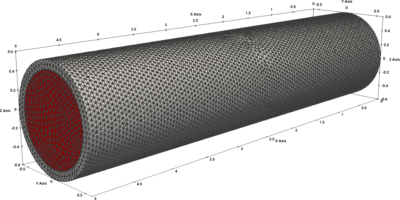
Figure 3. Example 3: the fine mesh with mesh size $h=0.05$. The red region is the fluid domain, and the gray region is the structure domain.

For the preconditioned MinRes linear system solver, we replace the point Gauss-Seidel smoother $\mathsf{R}$ in the velocity preconditioner (32) by a block Gauss-Seidel smoother $\mathsf{R}^{e}$ based on edge blocks to further improve its efficiency. We stop the MinRes iteration when residual norm is decreased by a factor of $10^{-6}$. The average number of iterations for convergence for $k=1$ with $h=0.05$ is $60$ and that for $k=2$ with $h=0.1$ is $52$ when the edge-block Gauss-Seidel smoother $\mathsf{R}^{e}$ is used in the velocity preconditioner (32). If we instead use the point Gauss-Seidel smoother, the numbers would be $360$ for $k=1$ and $246$ for $k=2$.

Similar to Example 2, we plot in Figure 4 the flow rate, which is calculated as two thirds of the horizontal velocity, and pressure at the center line $\{(x,0,0):\,x\in(0,5)\}$, and the y-component of the displacement on the interface line $\{(x,0.5,0):\,x\in(0,5)\}$ at final time $t=1.2\times 10^{-2}$. We find that the results for $k=1$ and $k=2$ agrees well with each other.

Figure 4. Example 3: Numerical solutions of the scheme (12) with different discretization parameters along cut lines at final time $t=1.2\times 10^{-2}[\mathsf{s}]$. Top: flow rate $\frac{2}{3}\hbox{\boldmath$v$}_{h}[0]$ along center line $\{(x,0,0):\,x\in(0,5)\}$; Middle: pressure along center line $\{(x,0,0):\,x\in(0,5)\}$; Bottom: y-component of displacement $\hbox{\boldmath$\eta$}^{s}_{h}[1]$ along the interface line $\{(x,0.5,0):\,x\in(0,5)\}$.

Finally, we plot the structure deformation along with the fluid pressure for $k=2$ with $h=0.1$ in Figure 5 for $t\in\{4,8,12\}\times 10^{-3}$. We clearly observe the propagation of a pressure pulse as time evolves.

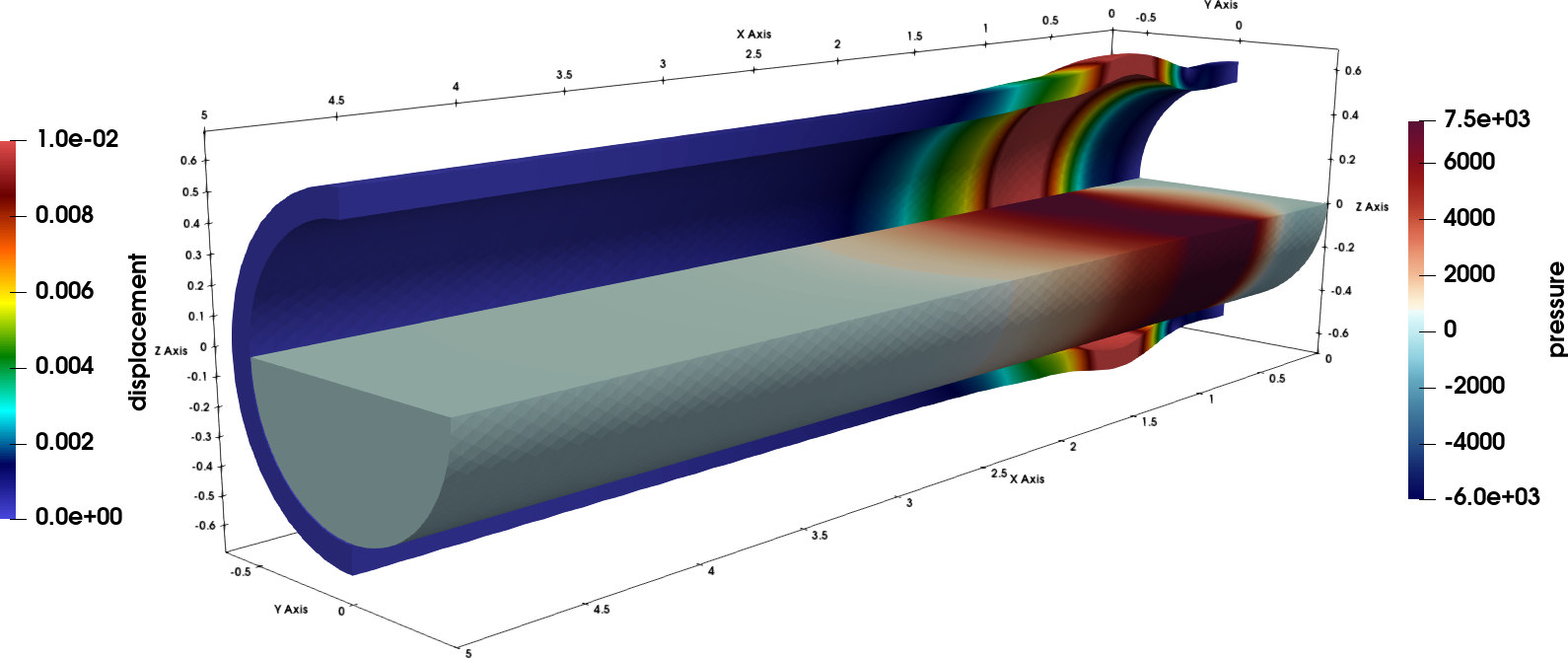
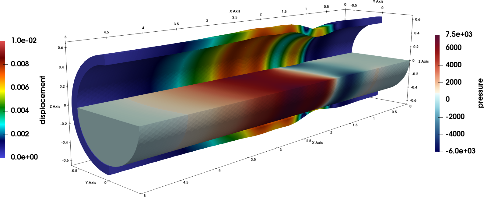
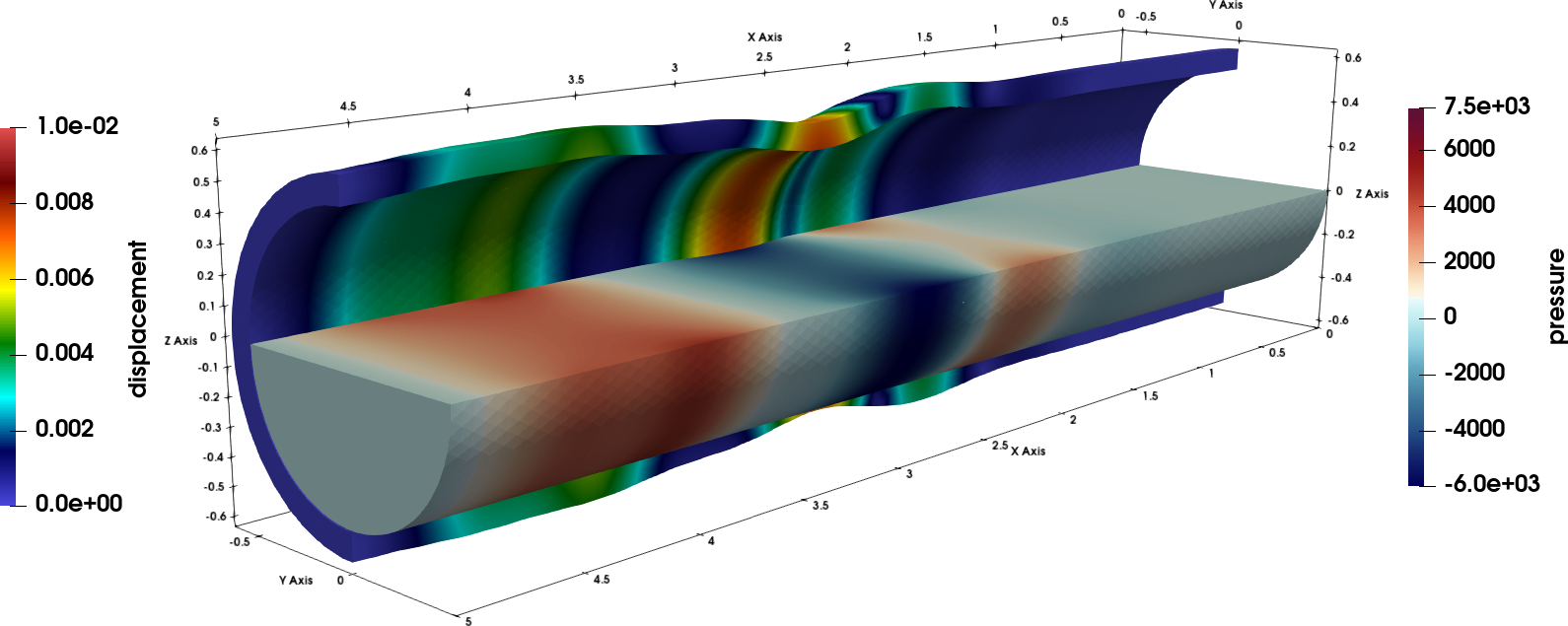
Figure 5. Example 3: The structure deformation and pressure approximation at different time. The structure deformation is enlarged by a factor of 8 and is only shown on half of the structure domain with $y<0$. The pressure approximation is only shown on half of the fluid domain with $z<0$. From top to bottom, $t=0.004,0.008,0.012$. ( $k=2$, $h=0.1$).

6. Conclusion

We have present a novel monolithic divergence-conforming HDG scheme for a linear FSI problem with a thick structure. The fully discrete scheme produces an exactly divergence-free fluid velocity approximation and is energy-stable. Furthermore, we design an efficient block AMG preconditioner and use it with a preconditioned MinRes solver for the resulting symmetric and indefinite global linear system. This preconditioner is numerically observed to be robust with respect to the mesh size, time step size and material parameters in large parameter ranges. A theoretical analysis of this preconditioner is our future work.

The extension of our scheme to other FSI models including thin structure and/or moving interfaces consists of our ongoing work.

References

• [1] M. Ainsworth and G. Fu, Fully computable a posteriori error bounds for hybridizable discontinuous Galerkin finite element approximations, J. Sci. Comput., 77 (2018), pp. 443–466.
• [2] S. Badia, A. Quaini, and A. Quarteroni, Modular vs. non-modular preconditioners for fluid–structure systems with large added-mass effect, Computer Methods in Applied Mechanics and Engineering, 197 (2008), pp. 4216–4232.
• [3] J. W. Banks, W. D. Henshaw, A. K. Kapila, and D. W. Schwendeman, An added-mass partition algorithm for fluid–structure interactions of compressible fluids and nonlinear solids, J. Comput. Phys., 305 (2016), pp. 1037–1064.
• [4] D. Boffi, F. Brezzi, M. Fortin, et al., Mixed finite element methods and applications, vol. 44, Springer, 2013.
• [5] J. H. Bramble and J. E. Pasciak, Iterative techniques for time dependent Stokes problems, vol. 33, 1997, pp. 13–30. Approximation theory and applications.
• [6] M. Bukac, A. Seboldt, and C. Trenchea, Refactorization of cauchy’s method: a second-order partitioned method for fluid-thick structure interaction problems, arXiv preprint arXiv:2008.12979, (2020).
• [7] M. Bukač, S. Čanić, R. Glowinski, B. Muha, and A. Quaini, A modular, operator-splitting scheme for fluid-structure interaction problems with thick structures, Internat. J. Numer. Methods Fluids, 74 (2014), pp. 577–604.
• [8] H.-J. Bungartz and M. Schäfer, Fluid-structure interaction: modelling, simulation, optimisation, vol. 53, Springer Science & Business Media, 2006.
• [9] J. Cahouet and J.-P. Chabard, Some fast $3$D finite element solvers for the generalized Stokes problem, Internat. J. Numer. Methods Fluids, 8 (1988), pp. 869–895.
• [10] P. Causin, J. Gerbeau, and F. Nobile, Added-mass effect in the design of partitioned algorithms for fluid-structure problems, Comput. Methods Appl. Mech. Engrg., 194 (2005), pp. 4506–4527.
• [11] B. Chabaud and B. Cockburn, Uniform-in-time superconvergence of hdg methods for the heat equation, Mathematics of Computation, 81 (2012), pp. 107–129.
• [12] S. K. Chakrabarti, Numerical models in fluid-structure interaction, WIT, 2005.
• [13] S. Deparis, M. Discacciati, G. Fourestey, and A. Quarteroni, Fluid-structure algorithms based on Steklov-Poincaré operators, Comput. Methods Appl. Mech. Engrg., 195 (2006), pp. 5797–5812.
• [14] E. H. Dowell and K. C. Hall, Modeling of fluid-structure interaction, Annual review of fluid mechanics, 33 (2001), pp. 445–490.
• [15] H. C. Elman, D. J. Silvester, and A. J. Wathen, Block preconditioners for the discrete incompressible Navier-Stokes equations, vol. 40, 2002, pp. 333–344. ICFD Conference on Numerical Methods for Fluid Dynamics, Part II (Oxford, 2001).
• [16] R. D. Falgout and U. M. Yang, HYPRE: a library of high performance perconditioners, In Preconditiners, Lecture Notes in Computer Science, pp. 632–641, 2002.
• [17] C. Farhat, K. G. Van der Zee, and P. Geuzaine, Provably second-order time-accurate loosely-coupled solution algorithms for transient nonlinear computational aeroelasticity, Computer methods in applied mechanics and engineering, 195 (2006), pp. 1973–2001.
• [18] M. A. Fernández and M. Landajuela, A fully decoupled scheme for the interaction of a thin-walled structure with an incompressible fluid, Comptes Rendus Mathematique, 351 (2013), pp. 161–164.
• [19] A. Figueroa, I. Vignon-Clementel, K. Jansen, T. Hughes, and C. Taylor, A coupled momentum method for modeling blood flow in three-dimensional deformable arteries, Comput. Methods Appl. Mech. Engrg., 195 (2006), pp. 5685–5706.
• [20] G. Fu, Uniform auxiliary space preconditioning for HDG methods for elliptic operators with a parameter dependent low order term, arXiv:2011.11828 [math.NA].
• [21]  , Arbitrary Lagrangian–Eulerian hybridizable discontinuous Galerkin methods for incompressible flow with moving boundaries and interfaces, Comput. Methods Appl. Mech. Engrg., 367 (2020), p. 113158.
• [22] G. Fu, C. Lehrenfeld, A. Linke, and T. Streckenbach, Locking free and gradient robust H(div)-conforming HDG methods for linear elasticity , arXiv:2001.08610 [math.NA].
• [23] M. W. Gee, U. Küttler, and W. A. Wall, Truly monolithic algebraic multigrid for fluid–structure interaction, International Journal for Numerical Methods in Engineering, 85 (2011), pp. 987–1016.
• [24] E. Hairer and G. Wanner, Solving ordinary differential equations. II, vol. 14 of Springer Series in Computational Mathematics, Springer-Verlag, Berlin, 2010.
• [25] V. E. Henson and U. M. Yang, BoomerAMG: a parallel algebraic multigrid solver and preconditioner, vol. 41, 2002, pp. 155–177. Developments and trends in iterative methods for large systems of equations—in memoriam Rüdiger Weiss (Lausanne, 2000).
• [26] G. Hou, J. Wang, and A. Layton, Numerical methods for fluid-structure interaction—a review, Communications in Computational Physics, 12 (2012), pp. 337–377.
• [27] B. Hübner, E. Walhorn, and D. Dinkler, A monolithic approach to fluid–structure interaction using space–time finite elements, Computer methods in applied mechanics and engineering, 193 (2004), pp. 2087–2104.
• [28] I. C. F. Ipsen, A note on preconditioning nonsymmetric matrices, SIAM J. Sci. Comput., 23 (2001), pp. 1050–1051.
• [29] T. Klöppel, A. Popp, U. Küttler, and W. A. Wall, Fluid–structure interaction for non-conforming interfaces based on a dual mortar formulation, Computer Methods in Applied Mechanics and Engineering, 200 (2011), pp. 3111–3126.
• [30] C. Lehrenfeld, Hybrid Discontinuous Galerkin methods for solving incompressible flow problems. Diploma Thesis, MathCCES/IGPM, RWTH Aachen, 2010.
• [31] C. Lehrenfeld and J. Schöberl, High order exactly divergence-free hybrid discontinuous Galerkin methods for unsteady incompressible flows, Comput. Methods Appl. Mech. Engrg., 307 (2016), pp. 339–361.
• [32] M. Lukáčová-Medvid’ová, G. Rusnáková, and A. Hundertmark-Zaušková, Kinematic splitting algorithm for fluid-structure interaction in hemodynamics, Comput. Methods Appl. Mech. Engrg., 265 (2013), pp. 83–106.
• [33] K.-A. Mardal and R. Winther, Uniform preconditioners for the time dependent Stokes problem, Numer. Math., 98 (2004), pp. 305–327.
• [34] M. F. Murphy, G. H. Golub, and A. J. Wathen, A note on preconditioning for indefinite linear systems, SIAM J. Sci. Comput., 21 (2000), pp. 1969–1972.
• [35] F. Nobile, Numerical approximation of fluid-structure interaction problems with application to haemodynamics, PhD thesis, École polytechnique fédérale de Lausanne, 2001.
• [36] F. Nobile and C. Vergara, An effective fluid-structure interaction formulation for vascular dynamics by generalized Robin conditions, SIAM J. Sci. Comput., 30 (2008), pp. 731–763.
• [37] M. A. Olshanskii, J. Peters, and A. Reusken, Uniform preconditioners for a parameter dependent saddle point problem with application to generalized Stokes interface equations, Numer. Math., 105 (2006), pp. 159–191.
• [38] T. Richter, Fluid-structure interactions: models, analysis and finite elements, vol. 118, Springer, 2017.
• [39] S. Rugonyi and K.-J. Bathe, On finite element analysis of fluid flows fully coupled with structural interactions, CMES- Computer Modeling in Engineering and Sciences, 2 (2001), pp. 195–212.
• [40] T. Rusten, P. S. Vassilevski, and R. Winther, Interior penalty preconditioners for mixed finite element approximations of elliptic problems, Math. Comp., 65 (1996), pp. 447–466.
• [41] Y. Saad, Iterative methods for sparse linear systems, Society for Industrial and Applied Mathematics, Philadelphia, PA, second ed., 2003.
• [42] J. Schöberl, C++11 Implementation of Finite Elements in NGSolve, 2014. ASC Report 30/2014, Institute for Analysis and Scientific Computing, Vienna University of Technology.
• [43] T. E. Tezduyar and S. Sathe, Modelling of fluid–structure interactions with the space–time finite elements: solution techniques, International Journal for Numerical Methods in Fluids, 54 (2007), pp. 855–900.
• [44] J. Xu, The auxiliary space method and optimal multigrid preconditioning techniques for unstructured grids, vol. 56, 1996, pp. 215–235. International GAMM-Workshop on Multi-level Methods (Meisdorf, 1994).