Mutual information for fermionic systems

Abstract

We study the behavior of the mutual information (MI) in various quadratic fermionic chains, with and without pairing terms and both with short- and long-range hoppings. The models considered include the short-range limit and long-range versions of the Kitaev model as well, and also cases in which the area law for the entanglement entropy is – logarithmically or non-logarithmically – violated. In all cases surveyed, when the area law is violated at most logarithmically, the MI is a monotonically increasing function of the conformal four-point ratio $x$. Where non-logarithmic violations of the area law are present, non-monotonic features can be observed in the MI and the four-point ratio, as well as other natural combinations of the parameters, is found not to be sufficient to capture the whole structure of the MI with a collapse onto a single curve. We interpret this behavior as a sign that the structure of peaks is related to a non-universal spatial configuration of Bell pairs. For the model exhibiting a perfect volume law, the MI vanishes identically. For the Kitaev model the MI is vanishing for $x\to 0$ and it remains zero up to a finite $x$ in the gapped case. In general, a larger range of the pairing corresponds to a reduction of the MI at small $x$. A discussion of the comparison with the results obtained by the AdS/CFT correspondence in the strong coupling limit is presented.

1 Introduction

Over the years, information theory has provided valuable tools to analyze and interpret many-body quantum systems. The entanglement entropy (EE), as measured by the von Neumann and Rènyi entropies, has quickly established itself as a standard benchmark that allows to discriminate different phases of matter and properties escaping traditional paradigms. EE provides relevant knowledge such as how much classical information is necessary for a faithful representation of a quantum system or as an efficient witness of critical behavior JPA2009 ; JSTAT2015 .

The EEs are bipartite measures, since they assess how much information is shared between two complementary subsystems of a system in a pure state (that is, with no intrinsic entropy as a whole). This information cannot be accessed by measurements on one part alone, as it reflects correlations between the two subsystems. Since correlations lie mostly on the boundaries between the subsystems, the area law, at most with logarithmic corrections, is typically obeyed Eisert10 .

To access additional information on the structure of multipartite entanglement and quantum correlations, multipartite measures have also been introduced. One such measure, although not an entanglement estimator, is the so-called mutual information (MI). The MI is typically tripartite. Starting with a system in a pure state, one indeed divides the system into two (non-overlapping) subsystems $A$ and $B$ and their complement $C\equiv\overline{A\cup B}$. The MI measures how much information on $A$ we can obtain by measuring $B$ (or vice-versa). Thus, the MI can be considered as a kind of two-point function, while, from this point of view, the EEs are essentially one-point functions. Note, however, that an alternative point of view is to start with a system made only of $A$ and $B$ in a mixed state obtained by tracing out $C$ and then to calculate the MI between $A$ and its complement $B=\overline{A}$. Comparing the two points of view, the latter can be considered as the result of removing $C$ and letting $A$ and $B$ be "immersed" in the bath constituted by $C$.

Taking this into account, in this work we will take the former approach and only consider pure tripartite systems, initializing the system under consideration in its (pure) ground state

$$\rho=\ket{\psi_{0}}\bra{\psi_{0}}.$$ (1)

We then divide the lattice in the three disjoint parts $A$, $B$ and their complement $C=\overline{A\cup B}$. The reduced density matrix of each subsystem is given by $\rho_{A}=tr_{B\cup C}\left\{\rho\right\}$, $\rho_{B}=tr_{A\cup C}\left\{\rho\right\}$, $\rho_{AB}=tr_{C}\left\{\rho\right\}$, and $\rho_{C}=tr_{A\cup B}\left\{\rho\right\}$, respectively. Starting from the von Neumann entropy of the subsystem $j$, defined as

$$S_{j}=-\,\mathrm{tr}\left\{\rho_{j}\ln\rho_{j}\right\},$$ (2)

(where $\rho_{j}$ is the reduced density matrix of the subsystem $j$), the MI between $A$ and $B$, denoted by $I_{(A,B)}$, is given by

$$I_{\left(A,B\right)}=S_{A}+S_{B}-S_{AB}\,.$$ (3)

The MI is positive and symmetric in $A$ and $B$. If $A$ and $B$ are complementary (that is $A\cup B$ equals the entire system) and the whole system is prepared into a pure state, then $S_{AB}\equiv S_{A\cup B}=0$ and $I_{(A,B)}=2S_{A}=2S_{B}$, thus the MI reduces to the von Neumann entropy. The MI satisfies an area law wolf08 and provides an upper bound to any two-point correlation function computed between $A$ and $B$:

$$I_{(A,B)}\geq{\Big{(}\langle{\cal O}_{A}\otimes{\cal O}_{B}\rangle-\langle{\cal O}_{A}\rangle\langle{\cal O}_{B}\rangle\Big{)}^{2}\over 2\left|{\cal O}_{A}\right|^{2}\left|{\cal O}_{B}\right|^{2}}\,.$$ (4)

Thus, the MI vanishes when no correlation exists between $A$ and $B$.

In the general case, $I_{(A,B)}$ is independent from UV cut-off parameters (since the divergences of the individual regions cancel over those of their union) and this is one of the properties that renders it more flexible over the entanglement entropy, for which it is sometime complicated to disentangle the physical from the cut-off contributions. Another limitation of the EE is that it makes sense as a measure only if the system is prepared in a pure state, while, as we remarked, the MI applies also to mixed state systems.

The MI can be considered as a kind of two-point function, since it depends on the relative position of regions $A$ and $B$. The MI is not a proper entanglement measure. However it is a measure of correlation between subsystems of a quantum system, and it quantifies the amount of information shared between the two regions, providing a quantum counterpart of the Shannon MI, which in general quantifies in suitable units the amount of information obtained about a random variable via the measurement of another random variable Mac .

The MI has been studied in several prototypical settings, starting from the Ising model um12 ; lau13 and critical chains alcaraz13 ; alcaraz14 ; stephan14 , in systems at finite temperature melko10 ; singh11 ; wilms11 ; iaconis13 ; bernigau15 and out of equilibrium growth ; eisler14 ; asplung14 ; alba17 ; gruber20 ; maity20 . Moreover, it has been used as a test for several phenomena, for instance in disordered systems getelina16 ; ruggiero16 ; detommasi17 and in the presence of spontaneous symmetry breaking hamma16 , and as well in the holographic settings headrick2010 ; vilaplana11 ; allais12 ; fischler13 . In one-dimensional (1D) systems described by a conformal field theory (CFT), several results have been obtained for the MI calculated with respect to the Shannon entropies (that is, basis-dependent entropies) alcaraz13 ; alcaraz14 ; stephan14 , while exact results in lattice systems have been obtained only in special cases brightmore19 . We refer to casini2009 for a review on the EE in free quantum field theory with disjoint intervals.

A general prediction for the behavior of the MI comes from the anti-de Sitter (AdS)/CFT-correspondence, in the strong-coupling (large conformal charge $c$) limit, where the MI has been found to behave as headrick2010 ; vilaplana11

$$I_{(A,B)}(x)=\begin{cases}0\,,\quad&x<1/2\\ \frac{c}{3}\log\frac{x}{1-x}\,,\quad&x\geq 1/2\end{cases}\,,$$ (5)

as a function of the conformal four-point ratio $x$, defined as

$$x=\frac{l^{2}}{\left(l+d\right)^{2}}\,,$$ (6)

where $l$ is the length (i.e., the number of sites) of the two subsystems $A$ and $B$ (taken to be the same size) and, assuming $A$ and $B$ both simply connected. In Eq. (6), $d$ is a distance between the two subsystems, being the minimum number of sites between two points belonging to $A$ and $B$. The four-point ratio is the traditional quantity used in CFT analysis DiFrancesco used to encode the position of the four edges of the two subsystems.

Most of the studies of MI have focused so far mostly on systems with short-range couplings/interactions. In this respect it would be interesting to compare results for long-range systems with the corresponding short-range findings, as motivated by recent results for quantum systems with long-range couplings where the effects of long-rangedness on critical properties, quantum dynamics and quantum entanglement properties have been studied celardo15 ; gong16 ; defenu16 ; defenu17 ; igloi18 ; blass18 ; defenu18 ; lerose19 ; pappalardi19 ; lerose20 . One of the models in which the features induced by long-range terms have been compared with their short-range counterparts is the long-range Kitaev model vodola14 ; vodola2016 ; Buyskikh16 ; vanregemortel16 ; lepori16 ; dutta17 ; lepori17 ; alecce17 ; defenu19 ; defenu19bis ; uhrich20 , where the pairing term present in the short-range chain $\sim\Delta c_{i}^{\dagger}c_{i+1}^{\dagger}$ kitaev has the form $\sim\Delta_{ij}c_{i}^{\dagger}c_{j}^{\dagger}$.

Our goal in the present paper is fourfold: i) to compare the short-range Kitaev model with the tight-binding chain to highlight the effect of the pairing term on the MI; ii) to study how short-range results for the MI get modified in the presence of long-range terms, analyzing the MI in several prototypical 1D chains with long-range hoppings and pairings; iii) to discuss the dependence of the MI on the physical parameters, and in particular on the conformal four-point ratio $x$, in the various models, including the Kitaev model; iv) to probe the, possibly different, behavior of the MI for systems displaying area law or its (non-logarithmic) violation for the EE. We will consider quadratic and translational invariant fermionic chains, allowing for the study of the MI for large system sizes peschel2011 . Before moving on with the presentation we observe that in general the conformal four-point ratio is not necessarily the correct quantity to use in the study of the MI, especially in gapped systems. It is anyway a useful combination of parameters that can be employed to compactly express the obtained results. In the following we will use $x$, as well as other parameters such as $l/d$ according to what we find more convenient in the different cases, commenting on other possible choices of combinations.

Regarding points i) and iii), we observe that although the models considered are not in the regime of validity for the AdS/CFT result (5), we aim at testing whether at least there is a qualitative agreement with it. We will show that, when the area law is violated more than logarithmically, the MI develops non-monotonic features, with peaks for small $x$, in contrast with (5). We will also argue that the four-point ratio is not sufficient to capture the structure of MI for systems with volume law of EE, indicating an incompatibility of these cases with the assumption of conformal invariance and thus, the failure of both the CFT and holographic predictions.

The plan of the paper is the following. In Section 2 we introduce the models we are going to consider, which comprise short and long-range, with and without pairing terms. Section 3 is devoted to the short-range models, with the tight-binding model considered in Section 3.1 and the Kitaev chain in 3.2. Long-range models are considered in Sections 4 and 5: in the former the long-range terms are the hopping ones, while in the latter we study the effect of long-range pairing terms. In Section 4 we consider different forms of hoppings, which are known to generate different phenomenologies in the EE scaling: hoppings decaying as a power-law exhibiting area law for the EE are considered in Section 4, while the MI for model with fractal Fermi surface having a scaling of EE intermediate between area and volume laws is discussed in Section 4.1. Models featuring EE volume law are studied in Section 4.2, where we consider both a long-range power-law model with a space-dependent phase in the hopping in Section 4.2.1 and models with selective hoppings in Section 4.2.2. Here the hopping is chosen in a way to reproduce a state with the maximum number of Bell pairs, therefore giving EE volume law. We focus in particular on the model in which each site is coupled by an hopping term to the most distant site, a model introduced in gori15 and to which we refer to as the "antipodal" model. Deviations from the antipodal model are as well investigated. Section 5 considers the case of long-range pairings, both with short-range hoppings (Section 5.1) and long-range hoppings (Section 5.2). The use of MI to detect quantum phase transitions in such models is studied. Final comments and conclusions drawn from our results are collected in Section 6.

2 The models

In this paper, we consider 1D fermionic models of the form

$$H=H_{H}+H_{P},$$ (7)

where $H_{H}$ is the hopping part and $H_{P}$ the pairing part of the Hamiltonian. Sites are labeled by indices $i,j=1,\cdots,N_{s}$ and $N_{S}$ is the number of sites. The fermionic operators creating and destroying a fermion on site $i$ are denoted by $c_{i}$ and $c_{i}^{\dagger}$, respectively. The filling $f$, which is also the number of particles per site, is defined as $f=N_{T}/N_{S}$, where $N_{T}=\sum_{i=1}^{N_{S}}c_{i}^{\dagger}c_{i}$ is the total particle number operator. As usual, the filling can be fixed directly or via the introduction of a chemical potential $\mu$, amounting to fixing the number of fermions from the Hamiltonian $H-\mu N_{T}$. We will consider as well translational invariant models, where, unless explicitly stated, periodic boundary conditions (PBC) are imposed (antiperiodic boundary conditions will be instead imposed when long-range pairing terms will be considered):

$$c_{i+N_{S}}\equiv c_{i}.$$ (8)

The hopping part $H_{H}$ of the Hamiltonian (7) reads in general

$$H_{H}=-\sum_{i,j=1}^{N_{S}}t_{i,j}c_{i}^{\dagger}c_{j}+\mathrm{H.c.},$$ (9)

where $t_{i,j}$ is the hopping amplitude among sites $i$ and $j$. Several form of $t_{i,j}$ will be considered:

• nearest-neighbor, with $t_{i,j}\neq 0$ for $j=i\pm 1$ and vanishing otherwise;

• selective hopping, with $t_{i,j}$ constant and non-vanishing if the distance between $i$ and $j$ is in an assigned interval of values. For instance, the antipodal model has $t_{i,j}\neq 0$ only if $|i-j|=N_{S}/2$ (with $N_{S}$ even).

• long-range with

  $$t_{i,j}\propto\frac{1}{|i-j|_{p}^{\alpha}}\,,$$ (10)

  where the distance $|\cdot|_{p}$, due to PBC, is defined as

  $$|i-j|_{p}=\min\left(|i-j|,N_{S}-|i-j|\right)\,.$$ (11)

  Notice that while in Sections 3.1 and 4 the prefactor not written in (10) is considered real, in the model discussed in Section 4.2.1 is complex.

The power-law exponent Eq. $\alpha$ in (10) is such that for $\alpha\to\infty$ the short-range limit is retrieved. Moreover, if $\alpha>d=1$ (more in general $\alpha$ larger than the dimension $d$ of the lattice) then the energy is extensive libro . When $\alpha>1$, in statistical mechanics models one can find a value of $\alpha$, often denoted by $\alpha^{*}$, such that for $\alpha>\alpha^{*}$ the critical behavior is the one of the short-range model sak1973 , although of course non-universal quantities may depend on $\alpha$ (see a review in review ). One refers often to the range $\alpha\leq 1$ as the "strong" long-range" region and to $1<\alpha<{\color[rgb]{0,0,0}\alpha^{*}=2}$ (for 1D chains) as the "weak" long-range region, but in this paper, not being crucially focused on critical properties, we will not make such distinction, making generic reference to the law (10) as a long-range, power-law decay. An important point emerging in the study of lattice models with long-range interactions is that critical properties change with the exponent $\alpha$ at a fixed dimension of the lattice in which interactions are long-range review . So, from this point of view, changing the dimension of the lattice (e.g., considering two-dimensional lattices), although interesting, is expected not to qualitatively change the properties we are going to discuss.

Since we are adopting PBC, the eigenfunctions of the matrix $-t_{i,j}$ are plane waves $\psi_{k}(j)\propto e^{ikj}$, with $k=\frac{2\pi}{N_{S}}n_{k}$ and $n_{k}=-N_{S}/2,\ldots,N_{S}/2-1$, again assuming $N_{S}$ even (the lattice spacing is set for simplicity $\equiv 1$). Therefore the hopping Hamiltonian (9) can be readily diagonalized as $H_{H}=\sum_{k}\epsilon_{k}c_{k}^{\dagger}c_{k}$, with $c_{k}$ the Fourier transform of $c_{i}$ and $\epsilon_{k}$ depending of course on the specific form of the $t_{i,j}$. In Section 4.1 a model with fractal Fermi surface is studied, and there the form of $\epsilon_{k}$ will be directly given without explicitly assigning the hoppings $t_{i,j}$.

For the hopping Hamiltonian (9) the EE of the subsystem $A$ having $l$ sites is given by peschel2011

$$S_{A}=-\sum_{\gamma=1}^{l}\left[\left(1-C_{\gamma}\right)\ln{\left(1-C_{\gamma}\right)}+C_{\gamma}\ln{C_{\gamma}}\right]\,.$$ (12)

In (12) the $C_{\gamma}$ are the $l$ eigenvalues of the correlation matrix

$$C_{ij}=\langle\Psi|c_{i}^{\dagger}c_{j}|\Psi\rangle\,,$$ (13)

with $i,j=1,\cdots,l$ being the sites belonging to $A$ and $\Psi$ the ground-state of the fermionic system.

To calculate the MI, we calculate the EE of two systems $A$ and $B$ having each $l$ sites, then the EE of $A\cup B$, and finally the MI using (5). In this way we can readily calculate and analyze the MI, and express it in term of the four-point ratio where $d$ is the (minimal) distance between $A$ and $B$. The results we are going to present in the following are obtained using PBC, in order to treat a larger number of sites, however we have also checked that open boundary conditions do not qualitatively alter the outcomes.

Let us now discuss the pairing term $H_{P}$ in the total Hamiltonian (7):

$$H_{P}=\sum_{i,j=1}^{N_{S}}\Delta_{i,j}c_{i}^{\dagger}c_{j}^{\dagger}+\mathrm{h.c.}\,.$$ (14)

When both the pairing term $\Delta_{i,j}$ and the hopping term are nearest-neighbor ($\neq 0$ only if $j=i\pm 1$ and zero otherwise), then one has the Kitaev model kitaev . Long-range in the pairings will be as well introduced:

$$\Delta_{i,j}\propto\frac{1}{|i-j|_{p}^{\alpha}},$$ (15)

both with short-range and long-range hopping $t_{i,j}$. The full Hamiltonian, being quadratic, can be readily diagonalized Blaizot , and we denote again by $\epsilon_{k}$ the corresponding eigenvalues. The EE of subsystems can be calculated from the matrices $t_{i,j}$ and $\Delta_{i,j}$, extending the result (12) valid when $\Delta_{i,j}=0$. In the presence of pairings, indeed, the von Neumann entropy between two subsystems $A$ and $B$, required to calculate the MI, has to be derived in a different way with respect to the case $\Delta_{i,j}=0$ when one uses Eq. (12). With $\Delta_{i,j}\neq 0$ the correlations $\langle c_{j}c_{l}\rangle$ and $\langle c_{j}^{\dagger}c^{\dagger}_{l}\rangle$ do not vanish in general. We thus need to enlarge the correlation matrix to double its size in order to account for the additional terms. To do so, one define a matrix $M_{p,q}\equiv\langle(a_{2p-1},a_{2p})(a_{2q-1},a_{2q})\rangle$, where $a_{2q-1}\equiv c_{q}+c_{q}^{\dagger}$ and $a_{2q}\equiv i\,(c_{q}-c_{q}^{\dagger})$ are Majorana fermions, and the indices $p,q=1,\dots,l$ run over the $l$ sites of subsystem $A$. The matrix ${\bf M}$ has $l$ pairs of eigenvalues $1\pm v_{n}$, in terms of which the EE is straightforwardly expressed as in (12). We refer to peschel2011 for a presentation of the calculation of the EE for a generic quadratic form of fermions and for more references on the subject.

3 Short-range models

In this Section we consider short-range models, with nearest-neghbor hopping and $\Delta_{i,j}=0$ (Section 3.1) or $\Delta_{i,j}$ nearest-neighbor as well (Section 3.2).

3.1 Tight-binding chain

The usual tight-binding chain Hamiltonian reads:

$$H=-t\sum_{i=1}^{N_{S}}c_{i}^{\dagger}c_{i+1}+\mathrm{H.c.}\,,$$ (16)

with the PBC (8), so that $c_{N_{S}+1}=c_{1}$. We will consider its generalization in eq. (9), with a hopping term of the form:

$$t_{i,j}=\frac{t}{|i-j|_{p}^{\alpha}}\,,$$ (17)

the nearest-neighbor case (16) being obtained in the limit $\alpha\to\infty$.

The reason for considering (17) is two-fold: i) the short-range behaviour is in general expected to be retrieved for large, finite $\alpha$; ii) as discussed in gori15 , the EE of a subsystem does not depend on the exponent $\alpha$. Indeed, the correlation matrix (13) can be written as $C_{i,j}=\sum_{l=1}^{N_{T}}\psi_{l}^{*}(i)\psi_{l}(j)$, where the $\psi_{\alpha}$ are the eigenfunctions of the matrix $t_{i,j}$. In the considered translationally invariant case, the quantum number $l$ becomes the wave vector $k$ and the eigenfunctions $\psi_{l}$ simply plane waves. So, if the dispersion relation $\epsilon_{k}$ has a purely monotonous behavior for $k$ either positive or negative, then the correlation matrix is the same (since one has to sum on the same eigenfunctions). Thus, also the eigenvalues of the correlation matrix $C_{i,j}$ are equal and so are the EE and, therefore, the MI as well.

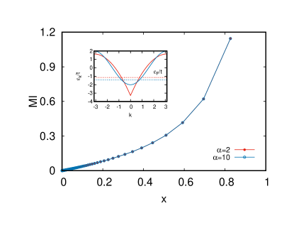
Figure 1: Plot of the MI as a function of the conformal four-point ratio (6) for the hopping $t_{i,j}=t/|i-j|_{p}^{\alpha}$ in the Hamiltonian (9) and two different values of $\alpha$: $\alpha=2$ and $\alpha=10$. As discussed in the text, checked numerically and seen in the figure, the MI does not depend on $\alpha$, and it is the same for the short-range limit (16). The plot refers to a chain of length $N_{S}=2004$, with PBC and filling fraction $f=0.25$. The four-point ratio is calculated varying the distance between two subsystems of the same length $l=10$. Inset: the two corresponding dispersion relations $\epsilon_{k}$ (in units of $t$) for $\alpha=2$ and $\alpha=10$, depicted together with their Fermi level. One sees that, even if the Fermi energies are different, the filled states are the same and, as a consequence, the MI is the same.

Since for any $\alpha$ in (17) the dispersion relation is indeed monotonous for $k$ either positive or negative, as seen in the inset of Fig. 1, the MI does not depend on $\alpha$. The main findings, valid therefore for any positive $\alpha$ in (17) and in particular for the short-range hopping model (16), are shown in Fig. 1 and Fig. 2. In Fig. 1 we plot the MI as a function of $x$. We see that the MI has a linear behavior for small $x$ and it is a monotonously increasing function of $x$.

In Fig. 2 the MI is reported for different values of the subsystems sizes $l$ at fixed $N_{S}$ and the same behavior appears for the considered cases. As supported also from simulations where the total length of the chain is varied, it is seen that the curves tends to converge to a monotonic function.

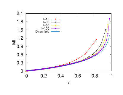
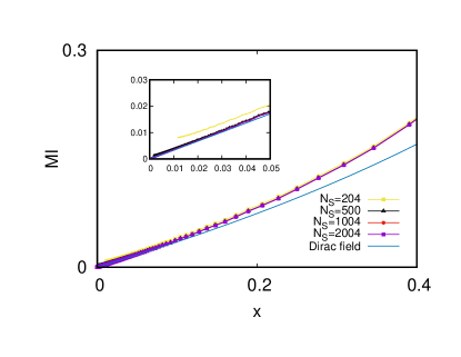
Figure 2: Top panel: MI for the chain (9) with hopping (17) with $\alpha=2$ and $N_{S}=2004$ for several values of the subsystem size $l$. Bottom panel: Scaling of MI with the number of sites $N_{S}$ for $l=10$. The blue continuous line represent the analytical prediction in eq. (18).

These results can be compared with the analytical values of the EE for disjoint subsystems of Dirac fermions, see casini2009 and refs. therein. This is done again in Fig. 2: the analytical values, given by

$$I=\frac{1}{3}\mathrm{log}\,\Big{(}\frac{1}{1-x}\Big{)},$$ (18)

are represented by the blue continuous line. We find a strongly improving agreement between numerics and analytics as $l$ increases. Moreover, for fixed $l$, a very good stability of the data is achieved for $N_{s}\sim 1000$.

Further analytical results would be desirable to determine the MI as a function of $x$ for intermediate and large values of $N_{S},l$, and $d$ at fixed filling to discuss finite-size corrections, however from the results presented here it emerges that $x$ is the good quantity to use, the MI being a monotonic function of $x$. The prediction (5) is clearly not verified, as expected.

3.2 Kitaev chain

We consider in this Section the Kitaev Hamiltonian

$$H=-t\sum_{i=1}^{N_{S}}\left(c^{\dagger}_{i}c_{i+1}+\mathrm{H.c.}\right)+\frac{\Delta}{2}\sum_{i,j=1}^{N_{S}}\frac{1}{|i-j|_{p}^{\alpha}}\left(c^{\dagger}_{j}c^{\dagger}_{i}+c_{i}c_{j}\right)\,.$$ (19)

focusing on the limit $\alpha\to\infty$. In this limit, one recovers the short-range Kitaev chain kitaev , that in turn can be mapped via Jordan-Wigner transformations to the Ising model in transverse field libro_cha .

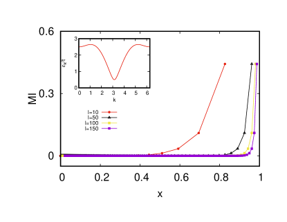
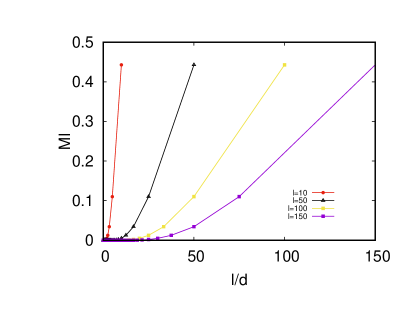
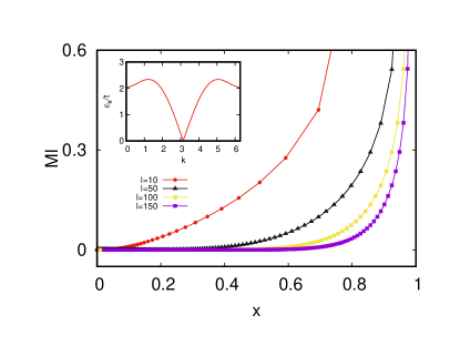
Figure 3: (Upper panel) Bogoliubov quasiparticle spectrum (inset) and MI as a function of the four-point ratio $x$ for the Kitaev chain (19) with $\alpha=1000$, using the parameters $N_{S}=2004$ and $\mu=1.5$ (corresponding to the filling $f=0.5567$). (Middle panel) Same, but now as a function of $l/d$. (Lower panel) Same as the upper panel, but for $\mu=1.05$.

For the model (19), it is convenient to work with anti-periodic boundary conditions vodola14 . To fix the average number of particles, we introduce a chemical potential by adding the term $-\mu\sum_{j=1}^{N_{S}}\left(c_{j}^{\dagger}c_{j}-\frac{1}{2}\right)$ to the Hamiltonian (19). To compare with previous results, without loss of generality, we will set $\Delta=2t=1$, since different choices can be absorbed in a redefinition of $\mu$, therefore measuring the energies in units of $2t$ vodola14 ; vodola2016 .

Presenting the results also for finite $\alpha$, the spectrum of excitations is obtained via a Bogoliubov transformation and it results in:

$$\epsilon_{k}=\sqrt{\left(\mu-\cos{k}\right)^{2}+f_{\alpha}^{2}(k+\pi)}\,,$$ (20)

where $k=-\pi+\frac{2\pi}{N_{S}}\left(n+\frac{1}{2}\right)$ ($0\leq n<N_{S}$) and

$$f_{\alpha}(k)\equiv\sum_{m=1}^{N_{S}-1}\frac{\sin(mk)}{|m|_{p}^{\alpha}}\,.$$ (21)

The functions $f_{\alpha}(k)$ become, in the thermodynamic limit vodola2016 ; lepori16 , a polylogarithmic function grad ; abr ; nist . The ground state of Eq. (19) is given by

$$\ket{\Omega}=\prod_{n=0}^{N_{S}/2-1}\left(\cos\theta_{k_{n}}-i\sin\theta_{k_{n}}\,{\color[rgb]{0,0,0}c^{\dagger}_{k_{n}}c^{\dagger}_{-k_{n}}}\right)|0\rangle\ ,$$ (22)

where $\tan(2\theta_{k_{n}})=-\frac{f_{\alpha}(k_{n}+\pi)}{\mu-\cos{k_{n}}}$ and it is even under the $Z_{2}$ fermionic number parity of the Hamiltonian muss ; fendley2012 .

The spectrum in (20) displays a critical line at $\mu=1$ for every $\alpha$ and a critical semi-line $\mu=-1$ for $\alpha>1$ (and therefore in the short-range Kitaev model $\alpha\to\infty$ as well).

We report in Fig. 3 the MI as a function of the conformal four-point ratio $x$ for $\alpha=1000$, practically indistinguishable from the short-range Kitaev model at $\alpha\to\infty$, $N_{S}=1000$ and $\mu=1.5$. In the inset of Fig. 3, we plot the corresponding spectrum $\epsilon_{k}$ for the Bogoliubov quasiparticles. In Fig. 3 we plot also MI as a function of $l/d$ for different values of $l$, and the comparison of the two panels shows that MI tends to be vanishing for small values of $x$ or $l/d$, or better up to certain value of them, and that collapse of data is not observed. In the considered ranges for the Hamiltonian parameters, the model satisfies an area law for the EE, and correspondingly the MI appears to vanish for $x<1/2$. However, the region in which MI vanished increases beyond $1/2$ approaching the thermodynamic limit.

Finally, studying the MI on the massless line $\mu=1$, one finds a monotonic growth of the MI with $x$, qualitatively equal to those in Figs. 1 and 2, and corresponding to a logarithmic violation of the area law by the von Neumann entropy. For completeness, in Fig. 3 we also report the MI close to the critical line (choosing $\mu=1.05$). There, a comparison with the predictions of the Dirac theory casini2009 , similarly as in the previous Section, would require a huge fine tuning of the Dirac mass.

4 Long-range hopping

In this Section we consider several models with long-range hopping.

For the model (9), without pairing terms ($\Delta_{i,j}=0$) and long-range hopping (17) given by $t_{i,j}=t/|i-j|_{p}^{\alpha}$, one can readily determine the energy spectrum as

$$\epsilon_{k}=-2t\,\ell_{\alpha}(k)\,,$$ (23)

where $k=2\pi n_{k}/N_{S}$ belongs to the first Brillouin zone, $n_{k}=-N_{S}/2,\cdots,N_{S}/2-1$, and

$$\ell_{\alpha}(k)=\sum_{n=1}^{\infty}\frac{\cos{(nk)}}{n^{\alpha}}\,.$$ (24)

As commented in Section 3.1, the dispersion relation (23) is monotonous in $k$ as in the short-range (see the inset of Fig. 1). The long-range hopping (17) only changes the values of the single-particle energies, and the MI is exactly the same as in the short-range model, as discussed in Section 3.1 and illustrated in Figs. 1 and 2. We conclude that long-rangedness is not enough to change the MI properties: one also needs (if pairing terms are absent) to change the behavior of the single-particle spectrum, and, in particular, the Fermi surface. This is discussed in the next Section.

4.1 Fractal Fermi surface

We assume here that the Hamiltonian is such that the single-particle energy spectrum has the form

$$\varepsilon_{k}=-t\sin{\left(\frac{1}{k^{\gamma}}\right)},$$ (25)

where $\gamma$ is a positive odd integer. Hamiltonian (25) is written in momentum space, and when written in real space the hopping $t_{ij}$ assumes a complicated and oscillating in sign form, having as a first approximation a power-law envelope. As shown in gori15 , at certain fillings, the Fermi surface of this model has a fractal topology. For instance, at half-filling $f=0.5$, the Fermi energy is zero, with the point $k=0$ being an accumulation point, see the bottom right inset of Fig. 4 . The Fermi surface has box counting dimension $d_{box}=\frac{\gamma}{\gamma+1}$, so that $d_{box}=1/2$ for $\gamma=1$. From finite size numerical data one sees that the EE violates the area law as $S_{A}\sim L^{\beta}$, where $\beta=d_{box}$ gori15 .

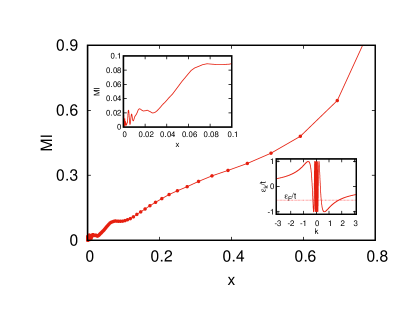
Figure 4: Plot of the MI as a function of the conformal four-point ratio $x$ for the chain with dispersion (25) and $\gamma=1$, $f=0.25$ and $N_{S}=1004$. The four-point ratio is calculated varying the distance between two subsystems of the same length $l=10$. In the top-left inset the small-$x$ region is enlarged. In the bottom-right inset dispersion is plotted with the Fermi level (dotted line).

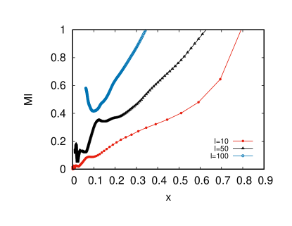
Figure 5: MI vs $x$ for the chain with dispersion (25) and $\gamma=1$, $f=0.25$ and $N_{S}=1004$. The four-point ratio is calculated varying the distance between two subsystems of the same length $l=10,20,50$.

Our results for the MI are reported in Figs. 4-6. The observed behavior differs from the previous models considered and displays very peculiar and unique features at small $x$. In Fig. 4 the MI as a function of $x$ is shown at a fixed value of $\gamma$. It is seen that the non-logarithmic violation of the area law makes the MI non-monotonous at small $x$. In Fig. 5 we plot the results obtained for different sizes of the subsystem size $l$: the MI does not seem to be dependent solely on the conformal four-point ratio $x$, since, in this model, varying the subsystems’ length produces different outcomes. Moreover, a non-logarithmic violation of the area law violates the basic assumption of holography and thus we cannot expect Eq. (5) to apply here, since both conformal invariance and AdS/CFT duality are not respected. Our numerical results support this conclusion. In Fig. 6, the MI is plotted for different values of $\gamma$, and thus of exponent $\beta$, defined after Eq. (25), which quantifies the deviation from the area law. We considered other combinations of system parameters different from $x$ such as $l/d$, but we found that they did not introduce a simplification of the obtained results and thus we do not presents plots of such results. It is found that the larger is the deviation from the area law, the more non-monotonic the MI is. Figure 6 also indicates that the Bell-pairs responsible for the EE have a specific distribution in space also at very large distances. Although an analytical determination of the peaks position in Figs. 4-5 is a very non-trivial task, we can qualitatively comment on their difference compared to the long-range model with a phase which we study in the following Section 4.2.1. In the latter case, the EE follows a volume law, while here the deviation from the area law is weaker and the fractal Fermi surfaces selects values of the momentum $k$ that do not necessarily alternate gori15 . Thus, the Bell pairs form not only close to antipodal sites but also between closer sites resulting in the complicated peak patterns observed in Figs. 4-5.

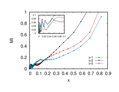
Figure 6: MI vs $x$ for the chain with dispersion (25) and $f=0.25$, $N_{S}=1004$ for different values of $\gamma$. The four-point ratio is calculated varying the distance between two subsystems of the same length $l=10$. In the top-left inset the small-$x$ region is enlarged.

4.2 Other models with non-logarithmic violations of the area law

Other models exhibiting non-logarithmic violations of the area law are considered in the following Sections 4.2.1 and 4.2.2. In both cases the pairing terms are absent, their effect being studied in Section 5.

4.2.1 Long-range power-law model with a phase

A possible way to modify the structure of the Fermi surface, is to introduce a space-dependent phase in the hopping matrix

$$t_{i,j}=\left\{\begin{array}[]{ll}0\,,&i=j,\\ \frac{te^{i\phi d(i-j)}}{|i-j|_{p}^{\alpha}}\,,&i\neq j\,,\end{array}\right.$$ (26)

where $\phi=\frac{2\pi}{N_{S}}\Phi$ (with $\Phi$ a constant) and $d(m)$ is the oriented distance, defined as

$$d(m)\equiv\left\{\begin{array}[]{ll}m&|m|\leq N_{S}-|m|,\\ {}\\ -N_{S}+|m|&{\rm otherwise}\,.\end{array}\right.$$ (27)

The energy spectrum is found to be $\epsilon_{k}=-2t\ell_{\alpha}(k)$ with

$$\ell_{\alpha}(k,\phi;N_{S})=\sum_{n=1}^{N_{S}/2}\frac{\cos{[n(k+\phi)]}}{n^{\alpha}}\,.$$ (28)

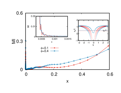
Figure 7: MI for the long-range model (9) with the phase-modulated hopping (26) with two values of the phase $\phi=0.1,0.4$ and parameters $N_{S}=1004$, $\alpha=0.3$, $l=10$, and $f=0.25$. Left inset: MI behaviour for small $x$. Right inset: energy spectrum for the two values of $\phi$.

While for $\phi=0$ this function is monotonic for $k\in[0,\pi]$, for non-zero $\phi$ there is a critical value of $\alpha_{c}(\phi)<1$ such that for $\alpha<\alpha_{c}(\phi)$, at half filling $f=1/2$, the energies (28) are rapidly oscillating and the momenta $k$ are occupied in an alternating way between even and odd quantum numbers, as depicted in the right panel of Fig. 7. As a consequence, a Bell-paired-like ground state is obtained, with a volume law EE gori15 . We notice that for $\alpha\leq 1$ the ground-state energy in the thermodynamic limit diverges. Nonetheless, one can make the energy extensive by the so-called Kac rescaling libro . As reported in Fig. 7, the MI shows a non-monotonic behavior with $x$, emerging at small $x$ (see left inset), where peaks develop. One also sees a clear peak at $x\to 0$. We attribute the presence of such non-monotonicity and peaks to the formation of Bell pairs, which are the reason for the (non-logarithmic) deviation from the area law. This will be more evident in the models studied in the following Section 4.2.2. Notice that by plotting MI as a function of $l/d$ we obtain similar results. Also for the long-range power-law model with a phase, as for the model of Section 4.1, the four-point ratio $x$ is found to be not sufficient to capture the whole structure of the MI, since as illustrated in Fig. 8, results with different values of $l$ but the same $x$ exhibit different results for the MI. However, non-monotonous behaviour and the increase for $x\to 0$ are seen.

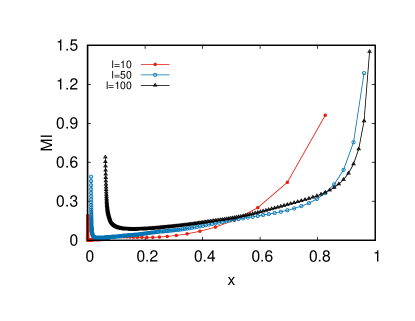
Figure 8: MI for the long-range model (9) with the phase-modulated hopping (26) for $N_{S}=1004$, $\alpha=0.3$, $f=0.25$, $\phi=0.1$ and different values of $l$.

4.2.2 Selective hopping

We study in this Section the "antipodal" model in which each-site is connected via a hopping term to the more distant site in the chain (at the antipodes). This model has a maximally entangled ground-state with the maximum number of Bell pairs, and it exhibits perfect, maximal volume law gori15 . As such, as we will shortly show, the MI vanishes identically, due to the monogamy of entanglement. To understand the role of deviations from a maximal volume law, we consider a chain with supplementary selective long-range hoppings, where the particle can only hop between sites centered around two distances, denoted by $s_{1,2}$, in a window of $2r+1$ sites ($r$ being an integer). The Hamiltonian reads

$$H=-\sum_{j=1}^{N_{S}}\sum_{q=-r}^{r}\left(t_{1}c_{j}^{\dagger}c_{j+s_{1}+q}+t_{2}c_{j}^{\dagger}c_{j+s_{2}+q}+\mathrm{H.c.}\right)\,,$$ (29)

where PBC are implied. This model is readily diagonalized in Fourier space, with energies

$$\epsilon_{k}=-2\Big{[}t_{1}\cos\left(ks_{1}\right)+t_{2}\cos\left(ks_{2}\right)\Big{]}\cos\left(kr\right)\left[1+\frac{\tan\left(kr\right)}{\tan\left(k/2\right)}\right]\ .$$ (30)

We now look at the MI for three specific cases:

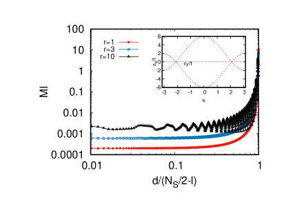
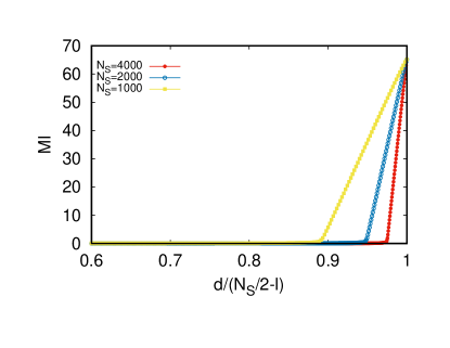
Figure 9: MI for the antipodal hopping model (29), with $s_{1}=N_{S}/2$ and $s_{2}=0$. Top panel: MI for $N_{S}=1000$ and $r=1,\,3,\,10$. Inset: energy spectrum for $r=1$. Bottom panel: MI for $N_{S}=1000,\,2000,\,4000$ and $r=1$.

Antipodal Hopping: $s_{1}=N_{S}/2$, $t_{2}=0$ ($t_{1}=t$): Let us first set $r=0$ (pure antipodal hopping). This means that we allow particles to hop only between the antipodal points and back (again, we take $N_{S}$ to be an even number). The single-particle spectrum reduces to

$$\epsilon_{k}=-2t\cos\left(\frac{kN_{S}}{2}\right)=-2t\left(-1\right)^{n_{k}}\ ,\quad k=\frac{2\pi}{N_{S}}n_{k}\ ,$$ (31)

which shows that there are two branches in the flat dispersion, with positive (negative) energy for odd (even) wave numbers. At half-filling, we thus have an alternating Fermi surface and an EE ruled by a perfect, maximal volume law. In fact, this choice of parameters creates a long-range Bell-paired state of maximal EE, since each particle is delocalized between two sites half-system apart. Remarkably, we find that such high entanglement content does not translate into the MI, which is in fact vanishing for any distance. This can be explained as a reflection of the entanglement monogamy coffman2000 ; osborne2006 of the model. Thus, one needs systems with a lower bipartite EE.

Allowing for $r\neq 0$ reduces the EE. For $r=1$ one has

$$\epsilon_{k}=-2t\left(-1\right)^{n_{k}}\left[1+2\cos\left(\frac{2\pi}{N_{S}}n_{k}\right)\right]\ .$$ (32)

Fig. 9 displays the MI for this case. Notice that here, and in the next Figs. 10 and 11 we prefer to plot MI not as a function of $x$, but of a scaled distance $d$ between the intervals. We see that the reduction in EE corresponds to a peak of MI close to $d=\frac{N_{S}}{2}-l$, almost vanishing otherwise. Oscillations in Fig.9 are really small and correspond to small variation of the entanglement due to longer hopping paths connecting the two partitions. The length of this path, and so the period $T$ of the oscillations, decreases with increasing $r$. It appears that $T\propto 1/r$

Single hopping with $s_{1}=s$, $t_{2}=0$ ($t_{1}=t$): Here we have the dispersion relation

$$\epsilon_{k}=-2t\cos\frac{2\pi s\>n_{k}}{N_{S}}$$ (33)

with $r=0$, and

$$\epsilon_{k}=-2t\cos\left(\frac{2\pi s\>n_{k}}{N_{S}}\right)\left[1+\frac{\tan\left(\frac{2\pi r\>n_{k}}{N_{S}}\right)}{\tan\left(\frac{\pi n_{k}}{N_{S}}\right)}\right]\cos\left(\frac{2\pi r\>n_{k}}{N_{S}}\right)$$ (34)

for general $r$, from which the Fermi surfaces can be worked out. The EE violates the area law and the MI is plotted for different values of $s$ in Fig. 10 for $r=0$. Similar results are found for other values of $r$ (not reported). One sees that there is a main peak corresponding to the Bell pair at the given $s$ where the maximum amount of Bell pairs is expected. Other secondary peaks appear at distances that are a multiple of $s$.

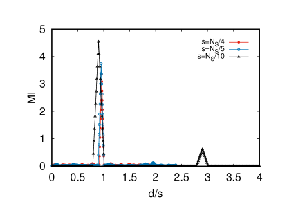
Figure 10: MI for the selected hopping model (29) with $t_{2}=0$, $f=0.5$, $r=0$ and different values $s=N_{S}/4,N_{S}/5,N_{S}/10$. We consider different chain lengths $N_{S}=900$ (top panel) and $1500$ (bottom panel).

Figure 11: MI for the selected hopping model (29) from any site only to two distant sites ($r=0$, $l=10$ and $f=0.5$) $s_{1}=N_{S}/4$ and $s_{2}=N_{S}/5$.

Hopping exactly to two distant sites with $r=0$: With hopping allowed only between sites with distances $s_{1}$ and $s_{2}$, one has

$$\epsilon_{k}=-2\left[t_{1}\cos\left(\frac{2\pi s_{1}\>n_{k}}{N_{S}}\right)+t_{2}\cos\left(\frac{2\pi s_{2}\>n_{k}}{N_{S}}\right)\right]\ .$$ (35)

For $s_{1}=N_{S}/2$ and $s_{2}=N_{S}/4$ at half-filling $f=1/2$, the single-particle spectrum is following a zig-zag behaviour, with odd wavenumber states filled in the ground state. As for the case of Fig. 9, this is a maximal EE case, where two particles are delocalized over four sites ($N_{S}/4$ apart), and the MI vanishes. In Fig. 11, we show the MI for $s_{1}=N_{S}/4$ and $s_{2}=N_{S}/5$, at half-filling $f=1/2$. The EE is lowered, but the MI shows peaks for $d=s_{1}$ , $d=s_{2}$ and multiple distances related to the corresponding Bell pairs.

We also considered the case $s_{1}=N_{S}/2-1,s_{2}=N_{S}/2+1$ ($t_{1}=t_{2}=t$) with $r=0$, i.e.

$$H=-t\sum_{j}\left(c_{j}^{\dagger}c_{j+\frac{N}{2}+1}+c_{j}^{\dagger}c_{j+\frac{N}{2}-1}+\mathrm{H.c.}\right),$$ (36)

with single-particle spectrum

$$\epsilon_{k}=-4t\left(-1\right)^{n_{k}}\cos\frac{2\pi}{N}n_{k}.$$ (37)

The MI is depicted in Fig. 12 and shows similarities with the case in Fig. 7, where one has indeed a volume law, but not the perfect (i.e., maximal) volume law.

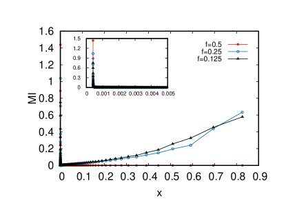
Figure 12: MI for the model (29) with hopping from any site only to the two sites surrounding the antipodal point ($s_{1,2}=N_{S}/2\pm 1$), with the right panel zooming the small $x$ behavior.

5 Long-range Kitaev chains

We consider in this Section the effect of a long-range counterpart of the fermionic pairing as given in Eq.(14), both in the presence of short-range (Section 5.1) and long-range (Section 5.2) hopping.

5.1 Short-range hopping and long-range pairing

Let us consider here long-range pairing ($\Delta_{i,j}=\frac{\Delta}{2|i-j|_{p}^{\alpha}|}$) and nearest-neighbour hopping ($t_{i,j}=t$ only if $i=j\pm 1$ and zero otherwise). The MI for the limit $\alpha\to\infty$ has been discussed in Section 3.2, where we also reported the energy spectrum for finite $\alpha$ in Eq. (20). As in Section 3.2 we consider $\Delta=2t$.

We remind that the spectrum (20) displays a critical line at $\mu=1$ for every $\alpha$ and a critical semi-line $\mu=-1$ for $\alpha>1$. Moreover, if $\mu\neq-1$ the velocity of quasiparticle with $k=\pm\pi$ diverges if $\alpha\leq\frac{3}{2}$, while it diverges at $\alpha\leq 2$ if $\mu=-1$ vodola14 . Below $\alpha=1$ and at every value of $\mu$, new phases occur vodola14 ; lepori2016 ; pezze2017 . There, the area law for the EE is logarithmically violated ares2015 ; lepori2016 . Moreover the boundary Majorana modes, present above $\alpha=1$ if $|\mu|<1$, become massive and disappear. Notably, this transition to the new phases at $\alpha=1$ occurs without any mass gap closure, as a consequence of the large space correlations induced by the long-range pairing. This transition is signaled by the ground-state fidelity pezze2017 .

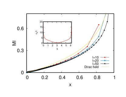
Figure 13: MI as a function of the four-point ration $x$ for the long-range Kitaev model with $\alpha=0.5$ and short-range hopping, with $N_{S}=1000$, $\mu=1.5$ (corresponding to an average occupation filling $f=0.5567$). Inset: Bogoliubov quasiparticle spectrum.

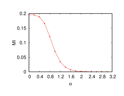
Figure 14: MI at $x=0.484$ for the long-range Kitaev model as a function of the decay exponent $\alpha$ for the pairing terms and short-range hopping, with $N_{S}=200$ and $\mu=1.5$.

Also for the MI, qualitatively different results are found passing through the line $\alpha=1$. We report in Fig. 13 the MI, as a function of the conformal four-point ratio $x$ for $\alpha=0.5$, for a closed chain with length $N_{S}=1000$ and $\mu=1.5$. In the inset, we plot the Bogoliubov spectrum $\epsilon_{k}$. For $\alpha\gtrsim 1$, the model satisfies an area law for the EE and the MI is qualitatively similar to that of Fig. 3: it appears to be vanishing for small $x$. Instead, for $\alpha\lesssim 1$, the EE is logarithmically violated, and the MI increases monotonically with $x$, qualitatively similar to that in Eq. (13). This is not due to the fact the model is gapless (see the inset), but rather to the fact that it has a such long-ranged pairing that the correlation functions are power-law decaying. This make the MI of the system similar to the tight-binding model studied in Sections 3.1 and 4.

Around the line $a=1$, the change in behaviour is smooth at finite size $N_{s}$, similarly to the EE vodola14 . This behaviour is shown in Fig. 14, where MI is reported as a function of $\alpha$ for a value of $x$ close to $1/2$. Finally, on the massless line $\mu=1$, also at $\alpha<1$, we find again a monotonic growth of the MI with $x$, similar to the short-range Kitaev chain.

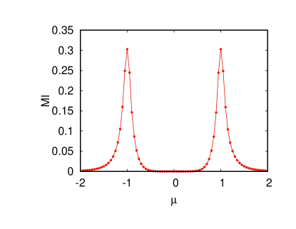
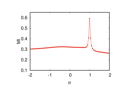
Figure 15: MI as a function of the chemical potential $\mu$ for the Kitaev chain with long-range pairing and short-range hopping with $\alpha=10$ (top) and $\alpha=0.5$ (bottom) and $N_{S}=2000$, $l=16$, and $d=4$ sites.

In Fig. 13, a comparison is made against the analytical values of the MI, derived from the EE for disjoint subsystems of Dirac fermions. We find that the agreement is rather poor. However, this mismatch is of course expected, since a Dirac structure does not hold for $\alpha<2$, not even around the massless (semi-)lines at $\mu=\pm 1$, where conformal invariance is broken by the long-range coupling lepori16 . We recall that instead the same Dirac structure holds around $\mu=\pm 1$ and for $\alpha>2$ muss .

The MI can be used to detect quantum phase transitions. To show this, we keep the four-point ratio fixed and swipe for the phase-diagram parameters $\mu$ and $\alpha$. In Fig. 15 we show in the top panel the MI as a function of $\mu$ for a chain with length $N_{S}=1000$, $l=16$, $d=4$, and $\alpha=10$. Two peaks are observed at $\mu=\pm 1$, in correspondence to the two critical points. Similarly, in the bottom panel we report the MI vs $\mu$ for $\alpha=0.5$ and the same choices for the other parameters. We observe a single peak, in correspondence to the unique critical point at $\mu=1$.
In Fig. 16 we plot the MI vs $\alpha$ for $\mu=0.5$ and $\mu=2.5$, and the other parameters as before. We observe a substantial increase for the MI for $\alpha\lesssim 1$, where the area law for the von Neumann entropy is logarithmically violated vodola14 ; lepori2016 . These properties are characteristic of phases at $\alpha<1$ that are not are not connected with those at $\alpha>1$ lepori2016 . For instance, they can host gapped edged modes, which are absent at $\alpha>1$. Moreover, these phases are not included in the standard classification of the (short-range) topological insulators and superconductors, due to the singularities in the Brillouin zone from the long-range couplings, see e.g. ludwig2009 .
Finally, for completeness we report in Fig. 17 the filling vs the chemical potential for different values of $\alpha$.

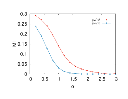
Figure 16: MI as a function of the power of long-range decay $\alpha$ of the pairing for $\mu=0.5$ and $\mu=2.5$ with $N_{S}=1000$, $l=16$, $d=4$ sites.

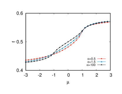
Figure 17: Filling vs chemical potential for different values of $\alpha$.

5.2 Long-range hopping and pairing

Finally, we consider the long-range paired Kitaev model with also long-range hopping:

$$H = -\sum_{i,j=1}^{N_{S}}\frac{t}{|i-j|_{p}^{\beta}}\left(c^{\dagger}_{i}c_{j}+\mathrm{H.c.}\right)-$$ (38)

$$-\sum_{i,j=1}^{N_{S}}\frac{\Delta}{2|i-j|_{p}^{\alpha}}\left(c_{j}^{\dagger}c_{i}^{\dagger}+c_{i}c_{j}\right)\,,$$

where we denote by $\beta$ ($\alpha$) the power-law decay exponent of the hopping (pairing) term.

We plot in Figs. 18 and 19 the MI as a function of $x$ for two different values of the pair $\alpha,\beta$ (with $N_{S}=1000$ and $\mu=1.5$). In the insets of both figures, the corresponding energy spectrum is plotted. In Fig. 18 we consider $\alpha=100$ and $\beta=0.5$, corresponding to a choice of short-range pairing and long-range hopping. In this case, it is seen that the spectrum of the Bogoliubov quasiparticles is regular, not fractal or "zig-zag", like the ones studied in Sections 4.1 and 4.2. The MI is vanishing for small $x$, paralleling the fulfillment of the EE area law, and conforming to the results obtained for the short-range Kitaev model. Instead, the case $\alpha=\beta=0.5$, with both long-range hopping and long-range pairing, is considered in Fig. 19. In this case, there are logarithmic violations for the EE area law and, correspondingly, we find that the MI is a monotonously increasing function of the conformal four-point ratio $x$, similar to the behaviors on massless semi(lines) $\mu\pm 1$, or in the regime $\alpha<1$, of the model in Eq. (19).

Figure 18: MI vs $x$ for the Kitaev chain (38) with non-local hopping and pairing. The parameters $\alpha=100$ and $\beta=0.5$, with $N_{S}=1000$ and $\mu=1.5$, are used. Inset: Bogoliubov quasiparticle spectrum.

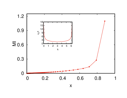
Figure 19: Same as in Fig. 18, but here $\alpha=\beta=0.5$.

6 Conclusions

We have studied the mutual information (MI) for several quadratic fermionic chains with a variety of different long-range hoppings and superconductive pairings, including the Kitaev model with short- and long-range pairings and the antipodal model in which the hoppings connect the most distant sites of the chain. The MI has been plotted as a function of the conformal four-point ratio $x$ and of other combinations of the physical parameters, such $l/d$ where $l$ and $d$ are respectively the length of and the distance between the two subsystems.

The conclusions emerging from the considered examples are the following. 1) When the area law is obeyed with at most logarithmic corrections, the MI is a monotonically increasing function of $x$, going to zero for $x\to 0$. 2) $x$ appears as a convenient variable for the critical short-range Kitaev model and the non-critical long-range Kitaev model, with small values of the exponent $\alpha$ (where the correlations have a power-law tail), in the sense that different values for the sizes of the system, of the subsystems and their distance with the same $x$ produces for large chains the same MI. However $x$ is not in general a variable for which MI data collapse, especially for not critical cases, and, as a rule of thumb, when $x$ is not a good variable, other combinations of parameters we tried are not either. 3) When there are non-logarithmic violation of the area law, the behaviour of MI vs $x$ is no longer monotonic and peaks appear, with the exception of the antipodal model in which MI vanishes identically, corresponding to a perfect, maximal volume law for the bipartite EE. 4) In these non-monotonic cases, $x$ does not capture the structure of the MI, since parameters with the same $x$ do not have the same MI (even though a similar qualitative behaviour is found).

The short-range Kitaev model in the massive regime exhibits a behaviour such that the MI is vanishing for small values of $x$, noticing however that we are outside of the range of validity for the AdS/CFT prediction (5). This result is actually independent from the short or long-range nature of the hopping. When the pairing becomes strongly long-range ($\alpha<1$), then the MI is no longer vanishing for small $x$ due to the power-law nature of the correlations induced by the long-range pairings. We point out that, as expected, for the Kitaev model we did not find a good agreement between our results for larger values of $x$ (say $x\gtrsim 1/2$) and the AdS/CFT prediction (5), since the latter is valid in the strong coupling limit. However, in both cases there is an overall monotonic growth of the MI as a function of the conformal four-point ratio $x$. For the considered Kitaev models, we showed the possibility to locate phase transitions using MI. Keeping the four-point ratio constant and sweeping the phase diagram, the MI displays distinct peaks at the closings of the gap, as shown in Figs. 15 and 16.

We also analyzed the MI behavior in systems with volume-like violations of the area law. We observed the emergence of peaks, and in particular for $x\simeq 0$, reflecting the structure of shared Bell-pairs between the subsystems. In fact, violations of the area law imply the formation of Bell pairs at arbitrary distances, growing with the thermodynamic limit. From this point of view we can then expect that in the infinite chain length limit, these peaks get squeezed toward $x\to 0$ (see Fig. 10). To analyze this behaviour we considered models with a controllable deviation from the perfect (i.e., maximal) volume law exhibited by the antipodal model. For the case of maximal volume law EE we found a vanishing MI (which can also be interpreted as a sign of entanglement monogamy) when the EE decreases the MI increases and peaks appear. The distribution of the latter is related to the formation of Bell-paired states at different distances, as it happens in the model with selective hopping considered in Section 4.2.2. A non-monotonic behaviour of the MI is observed, with features not being universal in terms of the four-point ratio. We can qualitatively explain this by the fact that a specific spatial distribution of Bell pairs cannot be simply captured by conformally invariant quantities.

The presented results show that the MI, even though not a proper entanglement measure, can be used to extract important information about the entanglement and quantum correlations properties and the phases of a quantum system. The peculiar role of long-range terms, as intertwined with the possible occurrence of violations of the area law, have been investigated and shown to produce a variety of interesting features. It would be certainly very interesting both to find analytical results for the behaviour of MI as a function of the conformal four-point ratio for some of the models considered here and to extend the analysis of the MI to interacting, non-quadratic models. Indeed, our results show that already for systems that can be mapped to free fermions the MI is not always captured by the existing analytical expressions. An interesting generalization and application of our study can be the use of MI as a scrambling quantifier (for dynamics under entangling unitary controls), for both open and closed quantum systems, in condensed matter (spin chains) as well as in high energy physics. This possibility has been highlighted recently in deffner2020_1 ; deffner2020_2 .

References

- (1) P. Calabrese, J. Cardy, and B. Doyon (eds.), Entanglement entropy in extended quantum systems, J. Phys. A 42 (2009).
- (2) S. Rachel, M. Haque, A. Bernevig, A. Laeuchli, and E. Fradkin (eds.), Quantum Entanglement in Condensed Matter Physics - Special Issue, J. Stat. Mech. (2015).
- (3) J. Eisert, M. Cramer, and M. B. Plenio, Colloquium: Area laws for the entanglement entropy, Rev. Mod. Phys. 82, 277 (2010).
- (4) M. M. Wolf, F. Verstraete, M. Hastings, and J. Cirac, Area Laws in Quantum Systems: Mutual Information and Correlations, Phys. Rev. Lett. 100, 070502 (2008).
- (5) D. J. C. MacKay, Information Theory, Inference, and Learning Algorithms (Cambridge, Cambridge University Press, 2003).
- (6) J. Um, H. Park, and H. Hinrichsen, Entanglement versus mutual information in quantum spin chains, J. Stat. Mech. P10026 (2012).
- (7) H. W. Lau and P. Grassberger, Information theoretic aspects of the two-dimensional Ising model, Phys. Rev. E 87, 022128 (2013).
- (8) F. C. Alcaraz and M. A. Rajabpour, Universal behavior of the Shannon mutual information of critical quantum chains, Phys. Rev. Lett. 111, 017201 (2013).
- (9) F. C. Alcaraz and M. A. Rajabpour, Universal behavior of the Shannon and Rényi mutual information of quantum critical chains, Phys. Rev. B 90, 075132 (2014).
- (10) J.-M. Stéphan, Shannon and Rényi mutual information in quantum critical spin chains, Phys. Rev. B 90, 045424 (2014).
- (11) R. G. Melko, A. B. Kallin, and M. B. Hastings, Finite-size scaling of mutual information in Monte Carlo simulations: Application to the spin- XXZ model, Phys. Rev. B 82, 100409(R) (2010).
- (12) R. R. P. Singh, M. B. Hastings, A. B. Kallin, and R. G. Melko, Finite-Temperature Critical Behavior of Mutual Information, Phys. Rev. Lett. 106, 135701 (2011).
- (13) J. Wilms, M. Troyer, and F. Verstraete, Mutual information in classical spin models, J. Stat. Mech. P10011 (2011).
- (14) J. Iaconis, S. Inglis, A. B. Kallin, and R. G. Melko, Detecting classical phase transitions with Renyi mutual information, Phys. Rev. B 87, 195134 (2013).
- (15) H. Bernigau, M. J. Kastoryano, and J. Eisert, Mutual information area laws for thermal free fermions, J. Stat. Mech. P02008 (2015).
- (16) J. Schachenmayer, B. P. Lanyon, C. F. Roos, and A. J. Daley, Entanglement Growth in Quench Dynamics with Variable Range Interactions, Phys. Rev. X 3, 031015 (2013).
- (17) V. Eisler and Z. Zimboras, Area law violation for the mutual information in a nonequilibrium steady state, Phys. Rev. A 89, 032321 (2014).
- (18) C. T. Asplund and A. Bernamonti, Mutual information after a local quench in conformal field theory, Phys. Rev. D 89, 066015 (2014).
- (19) V. Alba and P. Calabrese, Entanglement and thermodynamics after a quantum quench in integrable systems, PNAS 114, 7947 (2017).
- (20) M. Gruber and V. Eisler, Time evolution of entanglement negativity across a defect, J. Phys. A: Math. Theor. 53 205301 (2020).
- (21) S. Maity, S. Bandyopadhyay, S. Bhattacharjee, and A. Dutta, Growth of mutual information in a quenched one-dimensional open quantum many body system, Phys. Rev. B 101, 180301(R) (2020).
- (22) J. C. Getelina, F. C. Alcaraz, and J. A. Hoyos, Entanglement properties of correlated random spin chains and similarities with conformal invariant systems, Phys. Rev. B 93, 045136 (2016).
- (23) P. Ruggiero, V. Alba, and P. Calabrese, The entanglement negativity in random spin chains, Phys. Rev. B 94, 035152 (2016).
- (24) G. De Tomasi, S. Bera, J. H. Bardarson, and F. Pollmann, Quantum Mutual Information as a Probe for Many-Body Localization, Phys. Rev. Lett. 118, 016804 (2017).
- (25) A. Hamma, S. M. Giampaolo, and F. Illuminati, Mutual information and spontaneous symmetry breaking, Phys. Rev. A 93, 012303 (2016).
- (26) M. Headrick, Entanglement Renyi entropies in holographic theories, Phys. Rev. D 82 12 126010 (2010).
- (27) J. Molina-Vilaplana and P. Sodano, Holographic view on quantum correlations and mutual information between disjoint blocks of a quantum critical system, J. High Energy Phys. 2011, 11 (2011).
- (28) A. Allais and E. Tonni, Holographic evolution of the mutual information, J. High Energ. Phys. 2012, 102 (2012).
- (29) W. Fischler, A. Kundu,and S. Kundu, Holographic mutual information at finite temperature, Phys. Rev. D 87, 126012 (2013).
- (30) L. Brightmore, G. P. Geher, A. R. Its, V. E. Korepin, F. Mezzadri, M. Y. Mo, and J. A. Virtanen, Entanglement entropy of two disjoint intervals separated by one spin in an XX quantum spin chain, J. Phys. A: Math. Theor. 53 345303 (2020).
- (31) H. Casini and M. Huerta, Entanglement entropy in free quantum field theory, J. Phys. A: Math. Theor. 42, 504007 (2009).
- (32) P. Di Francesco, P. Mathieu, and D. Sénéchal, Conformal field theory (New York, Springer, 1997).
- (33) G. L. Celardo, R. Kaiser, and F. Borgonovi, Shielding and localization in the presence of long-range hopping, Phys. Rev. B 94, 144206 (2016).
- (34) Z. X. Gong, M. F. Maghrebi, A. Hu, M. Foss-Feig, P. Richerme, C. Monroe, and A. V. Gorshkov, Kaleidoscope of quantum phases in a long-range interacting spin-1 chain, Phys. Rev. B 93, 205115 (2016).
- (35) N. Defenu, A. Trombettoni, and S. Ruffo, Anisotropic long-range spin systems, Phys. Rev. B 94, 224411 (2016).
- (36) N. Defenu, A. Trombettoni, and S. Ruffo, Criticality and phase diagram of quantum long-range O(N) models, Phys. Rev. B 96, 104432 (2017).
- (37) F. IglóiF, B. Bla, G. Roósz G, and H. Rieger, Quantum XX model with competing short- and long-range interactions: Phases and phase transitions in and out of equilibrium, Phys. Rev. B 98, 184415 (2018).
- (38) B. Bla, H. Rieger, G. Roósz, and F. Iglói, Quantum relaxation and metastability of lattice bosons with cavity-induced long-range interactions, Phys. Rev. Lett. 121, 095301 (2018).
- (39) N. Defenu, T. Enss, M. Kastner, and G. Morigi, Dynamical Critical Scaling of Long-Range Interacting Quantum Magnets, Phys. Rev. Lett. 121, 240403 (2018).
- (40) A. Lerose, B. Zunkovic, A. Silva, and A. Gambassi, Quasi-localized excitations induced by long-range interactions in translationally-invariant quantum spin chains, Phys. Rev. B 99, 121112(R) (2019).
- (41) S. Pappalardi, P. Calabrese, and G. Parisi, Entanglement entropy of the long-range Dyson hierarchical model, J. Stat. Mech. 073102 (2019).
- (42) A. Lerose and S. Pappalardi, Origin of the slow growth of entanglement entropy in long-range interacting spin systems, Phys. Rev. Res. 2, 012041(R) (2020).
- (43) D. Vodola, L. Lepori, E. Ercolessi, A. V. Gorshkov, and G. Pupillo, Kitaev Chains with Long-Range Pairing, Phys. Rev. Lett. 113, 156402 (2014).
- (44) D. Vodola, L. Lepori, E. Ercolessi, and G. Pupillo, Long-range Ising and Kitaev Models: Phases, Correlations and Edge Modes, New J. Phys. 18, 015001 (2016).
- (45) A. S. Buyskikh, M. Fagotti, J. Schachenmayer, F. Essler, and A. J. Daley, Entanglement growth and correlation spreading with variable-range interactions in spin and fermionic tunneling models, Phys. Rev. A 93, 053620 (2016).
- (46) M. Van Regemortel, D. Sels, and M. Wouters, Information propagation and equilibration in long-range Kitaev chains, Phys. Rev. A 93, 032311 (2016).
- (47) L. Lepori, D. Vodola, G. Pupillo, G. Gori, and A. Trombettoni, Effective theory and breakdown of conformal symmetry in a long-range quantum chain, Ann. Phys. 374, 35 (2016).
- (48) A. Dutta and A. Dutta, Probing the role of long-range interactions in the dynamics of a long-range Kitaev chain, Phys. Rev. B 96, 125113 (2017).
- (49) L. Lepori, A. Trombettoni, and D. Vodola, Singular dynamics and emergence of nonlocality in long-range quantum models, J. Stat. Mech. 033102 (2017).
- (50) A. Alecce and L. Dell’Anna, Extended Kitaev chain with longer-range hopping and pairing, Phys. Rev. B 95, 195160 (2017).
- (51) N. Defenu, T. Enss, and J. C. Halimeh, Dynamical criticality and domain-wall coupling in long-range Hamiltonians, Phys. Rev. B 100, 014434 (2019).
- (52) N. Defenu, G. Morigi, L. Dell’Anna, and T. Enss, Universal dynamical scaling of long-range topological superconductors, Phys. Rev. B 100, 184306 (2019).
- (53) P. Uhrich, N. Defenu, R. Jafari, and J. C. Halimeh, Out-of-equilibrium phase diagram of long-range superconductors, Phys. Rev. B 101, 245148 (2020).
- (54) A. Y. Kitaev, Unpaired Majorana fermions in quantum wires, Phys.-Usp. 44, 131 (2001).
- (55) I. Peschel, Entanglement in solvable many-particle models, Braz. J. Phys. 42, 267 (2012).
- (56) G. Gori, S. Paganelli, A. Sharma, P. Sodano, and A. Trombettoni, Explicit Hamiltonians inducing volume law for entanglement entropy in fermionic lattices, Phys. Rev. B 91 245138 (2015).
- (57) A. Campa, T. Dauxois, D. Fanelli, and S. Ruffo, Physics of long-range interacting systems (Oxford, Oxford University Press, 2014).
- (58) J. Sak, Recursion Relations and Fixed Points for Ferromagnets with Long-Range Interactions, Phys. Rev. B 8, 281 (1973).
- (59) N. Defenu, A. Codello, S. Ruffo, and A. Trombettoni, Criticality of Spin Systems with Weak Long-Range Interactions, J. Phys. A: Math. Theor. 53, 143001 (2020).
- (60) J.-P. Blaizot and G. Ripka, Quantum theory of finite systems (Cambridge, MIT Press, 1986).
- (61) A. Dutta, G. Aeppli, B. K. Chakrabarti, U. Divakaran, T. F. Rosenbaum, and D. Sen, Quantum Phase Transitions in Transverse Field Models (Cambridge, Cambridge University Press, 2015).
- (62) I. S. Gradshteyn and I. M. Ryzhik, Tables of Integrals, Series, and Products (Amsterdam, Elsevier, 2007).
- (63) M. Abramowitz and I. A. Stegun, Handbook of Mathematical Functions (New York, Dover, 1964).
- (64) F. W. J. Olver, D. W. Lozier, R. F. Boisvert, and C. W. Clark, NIST Handbook of Mathematical Functions (Cambridge, Cambridge University Press, 2010).
- (65) G. Mussardo, Statistical Field Theory: An Introduction to Exactly Solved Models in Statistical Physics (Oxford, Oxford University Press, 2010).
- (66) P. Fendley, Parafermionic edge zero modes in Zn-invariant spin chains, J. Stat. Mech. P11020 (2012).
- (67) V. Coffman, J. Kundu, and W. K. Wootters, Distributed entanglement, Phys. Rev. A 61, 052306 (2000).
- (68) T. J. Osborne and F. Verstraete, General Monogamy Inequality for Bipartite Qubit Entanglement, Phys. Rev. Lett. 96, 220503 (2006).
- (69) L. Lepori and L. Dell’Anna, Long-range topological insulators and weakened bulk-boundary correspondence, New J. Phys. 19, 103030 (2017).
- (70) L. Pezzé, M. Gabbrielli, L. Lepori, and A. Smerzi, Multipartite entanglement in topological quantum phases, Phys. Rev. Lett. 119, 250401 (2017).
- (71) F. Ares, J. G. Esteve, F. Falceto, and A. R. de Queiroz, Entanglement in fermionic chains with finite-range coupling and broken symmetries, Phys. Rev. A 92, 042334 (2015).
- (72) A. P. Schnyder, S. Ryu, A. Furusaki, and A. W. W. Ludwig, Classification of Topological Insulators and Superconductors, AIP Conf. Proc. 1134, 10 (2009). arXiv:0905.2029.
- (73) A. Touil and S. Deffner, Quantum scrambling and the growth of mutual information, Quantum Sci. Technol. 5 035005 (2020).
- (74) A. Touil and S. Deffner, Information scrambling vs. decoherence – two competing sinks for entropy, PRX Quantum 2, 010306 (2021).